A Joint Typicality Approach to Algebraic Network Information Theory

Sung Hoon Lim, Chen Feng, Adriano Pastore,
Bobak Nazer, and Michael Gastpar
This paper was presented in part at the 2014 IEEE Information Theory Workshop, Hobart, Australia and the 2015 Allerton Conference on Communication, Control, and Computing, Monticello, IL.Sung Hoon Lim, Adriano Pastore, and Michael Gastpar are with the School of Computer and Communication Sciences, Ecole Polytechnique Fédérale, 1015 Lausanne, Switzerland (e-mail: sung.lim@epfl.ch, adriano.pastore@epfl.ch, michael.gastpar@epfl.ch).Chen Feng is with the School of Engineering, The University of British Columbia, Kelowna, BC, Canada (e-mail: chen.feng@ubc.ca).Bobak Nazer is with the Department of Electrical and Computer Engineering, Boston University, Boston, MA (e-mail: bobak@bu.edu).
Abstract

This paper presents a joint typicality framework for encoding and decoding nested linear codes for multi-user networks. This framework provides a new perspective on compute–forward within the context of discrete memoryless networks. In particular, it establishes an achievable rate region for computing the weighted sum of nested linear codewords over a discrete memoryless multiple-access channel (MAC). When specialized to the Gaussian MAC, this rate region recovers and improves upon the lattice-based compute–forward rate region of Nazer and Gastpar, thus providing a unified approach for discrete memoryless and Gaussian networks. Furthermore, this framework can be used to shed light on the joint decoding rate region for compute–forward, which is considered an open problem. Specifically, this work establishes an achievable rate region for simultaneously decoding two linear combinations of nested linear codewords from $K$ senders.

Index Terms:
Linear codes, joint decoding, compute–forward, multiple-access channel, relay networks

I Introduction

In network information theory, random i.i.d. ensembles serve as the foundation for the vast majority of coding theorems and analytical tools. As elegantly demonstrated by the textbook of El Gamal and Kim [1], the core results of this theory can be unified via a few powerful packing and covering lemmas. However, starting from the many–help–one source coding example of Körner and Marton [2], it has been well-known that there are coding theorems that seem to require random linear ensembles, as opposed to random i.i.d. ensembles. Recent efforts have demonstrated that linear and lattice codes can yield new achievable rates for relay networks [3, 4, 5, 6, 7, 8, 9], interference channels [10, 11, 12, 13, 14, 15, 16], distributed source coding [17, 18, 19, 20, 21], dirty-paper multiple-access channels [22, 23, 24, 25], and physical-layer secrecy [26, 27, 28]. See [29] for a survey of lattice-based techniques for Gaussian networks.

Although there is now a wealth of examples that showcase the potential gains of random linear ensembles, it remains unclear if these examples can be captured as part of a general framework, i.e., an algebraic network information theory, that is on par with the well-established framework for random i.i.d. ensembles. The recent work of Padakandla and Pradhan [30, 25, 16] has taken important steps towards such a theory, by developing joint typicality encoding and decoding techniques for nested linear code ensembles. In this paper, we take further steps in this direction by developing coding techniques and error bounds for nested linear code ensembles. For instance, we provide a packing lemma for analyzing the performance of linear codes under simultaneous joint typicality decoding (in Sections LABEL:sec:comp-finite and LABEL:sec:k-mac-proof) and a Markov Lemma for linear codes (in Appendix LABEL:app:ML-LC).

We will use the compute–forward problem as a case study for our approach. As originally stated in [5], the objective in this problem is to reliably decode one or more linear combinations of the messages over a Gaussian multiple-access channel (MAC). Within the context of a relay network, compute–forward allows relays to recover linear combinations of interfering codewords and send them towards a destination, which can then solve the resulting linear equations for the desired messages. Recent work has also shown that compute–forward is useful in the context of interference alignment. For instance, Ordentlich et al. [13] approximated the sum capacity of the symmetric Gaussian interference channel via compute–forward. The achievable scheme from [5] relies on nested lattice encoding combined with “single-user” lattice decoding, i.e., each desired linear combination is recovered independently of the others. Subsequent efforts [31, 13, 32] developed a variation of successive cancellation for decoding multiple linear combinations.

In this paper, we generalize compute–forward beyond the Gaussian setting and develop single-letter achievable rate regions using joint typicality decoding. Within our framework, each encoder maps its message into a vector space over a field and the decoder attempts to recover a linear combination of these vectors. In particular, Theorem 1 establishes a rate region for recovering a finite-field linear combination over a MAC. This includes, as special cases, the problem of recovering a finite-field linear combination over a discrete memoryless (DM) MAC and a Gaussian MAC. In Theorem 2, we develop a rate region for recovering an integer-linear combination of bounded, integer-valued vectors. Finally, in Theorem 3, we use a quantization argument to obtain a rate region for recovering an integer-linear combination of real-valued vectors.

As mentioned above, the best-known rate regions for lattice-based compute–forward rely on successive cancellation decoding. One might expect that simultaneous decoding yields a larger rate region for recovering two or more linear combinations. However, for a random lattice codebook, a direct analysis of simultaneous decoding is challenging, due to the statistical dependencies induced by the shared linear structure [33]. We are able to surmount this difficulty by carefully partitioning error events directly over the finite field from which the codebook is drawn. Overall, we obtain a rate region for simultaneously recovering two linear combinations in Theorem 4.

Our results recover and improve upon the rate regions of [5, 34, 32], thus providing a unified approach to compute–forward over both DM and Gaussian networks. Additionally, the single-letter rate region implicitly captures recent work [35, Example 3] that has shown that Gaussian input distributions are not necessarily optimal for Gaussian networks. One appealing feature of our approach is that the first-order performance analysis uses steps that closely resemble those used for random i.i.d. ensembles. However, there are several technical subtleties that arise due to linearity, which require careful treatment in our error probability bounds.

Refer to caption
Figure 1: An illustration of the typicality of random i.i.d. (red) and random linear (blue) codewords. Due to the weak law of large numbers, most random i.i.d. codewords are typical for large $n$. In contrast, since random linear codewords are uniformly distributed, exponentially many codewords will be atypical with respect to non-uniform distributions. We resolve this issue via multicoding, i.e., we generate exponentially more linear codewords than needed and use an auxiliary index to select the typical ones.

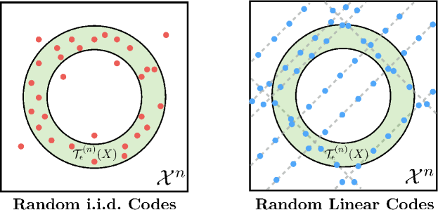
For a random linear codebook, each codeword is i.i.d. uniformly distributed over the underlying finite field. This poses a challenge for generating non-uniform channel input distributions, and it is well-known that a direct application of a linear codebook cannot attain the point-to-point capacity in general [36]. See Figure 1 for an illustration. To get around this issue, we will use the nested linear coding architecture which first appeared in [37, 38]. This encoding architecture consists of the following components:

  1. 1.

    an auxiliary linear code (shared by all encoders)

  2. 2.

    a joint typicality encoder for multicoding

  3. 3.

    a symbol-by-symbol function of the auxiliary linear codeword.

Roughly speaking, the auxiliary linear code is designed at a higher rate than the target achievable rate, the joint typicality encoding is used to select codewords of the desired type, and the function is used to map the codeword symbols from the finite field to the channel input alphabet. The idea of using a joint typicality encoder for channel coding appears in the celebrated coding scheme by Gelfand and Pinsker [39] for channels with state, Marton’s coding scheme for the broadcast channel [40] and the hybrid coding scheme [41] for joint–source channel coding. In contrast to these applications, our joint typicality encoding step is used to find an auxiliary codeword that is itself typical with respect to a desired distribution, instead of with respect to a state or source sequence. The use of a symbol-by-symbol function is reminiscent of the Shannon strategy [42] for channels with states.

The shared linear codebook creates subtle issues for the analysis of joint typicality encoding and decoding. Specifically, the users’ choices of typical codewords depend upon the codebook, and thus the codewords are not independent across users. For this scenario, the standard Markov lemma (see, for instance, [1, Lemma 12.1]) does not directly apply. To overcome this issue, prior work by Padakandla and Pradhan proposed a Markov lemma for nested linear codes that required both a lower and an upper bound on the auxiliary rates [25]. In Appendix LABEL:app:ML-LC, we follow a different proof strategy, which enables us to remove the upper bound.

Furthermore, for a random linear codebook, the codewords are only pairwise independent. While this suffices to apply a standard packing lemma [1, Section 3.2] for decoding a single codeword, it creates obstacles for decoding multiple codewords. In particular, one has to contend with the fact that competing codewords may be linearly dependent on the true codewords. To cope with these linear dependencies, we develop a packing lemma for nested linear codes, which serves as a foundation for the achievable rate regions described above.

We closely follow the notation in [1]. Let $\mathcal{X}$ denote the alphabet and $x^{n}$ a length-$n$ sequence whose elements belong to $\mathcal{X}$ (which can be either discrete or a subset of $\mathbb{R}$). We use uppercase letters to denote random variables. For instance, $X$ is a random variable that takes values in $\mathcal{X}$. We follow standard notation for probability measures. Specifically, we denote the probability of an event $\mathcal{A}$ by $\operatorname{\sf P}\{\kern 0.5pt\mathcal{A}\}$ and use $P_{X}(x)$, $p_{X}(x)$, $f_{X}(x)$, and $F_{X}(x)$ to denote a probability distribution (i.e., measure), probability mass function (pmf), probability density function (pdf), and cumulative distribution function (cdf), respectively.

For finite and discrete $\mathcal{X}$, the type of $x^{n}$ is defined to be $\pi(x|x^{n}):=\big{|}\{\kern 0.5pti:x_{i}=x\}\big{|}/n$ for $x\in\mathcal{X}$. Let $X$ be a discrete random variable over $\mathcal{X}$ with probability mass function $p_{X}(x)$. For any parameter $\epsilon\in(0,1)$, we define the set of $\epsilon$-typical $n$-sequences $x^{n}$ (or the typical set in short) [43] as ${\mathcal{T}_{\epsilon}^{(n)}}(X)=\{\kern 0.5ptx^{n}:|\pi(x|x^{n})-p_{X}(x)|\leq\epsilon p_{X}(x)\text{ for all }x\in\mathcal{X}\}$. We use $\delta(\epsilon)>0$ to denote a generic function of $\epsilon>0$ that tends to zero as $\epsilon\to 0$. One notable departure is that we define sets of message indices starting at zero rather than one, $[n]:=\{\kern 0.5pt0,\ldots,n-1\}$.

We use the notation $\mathbb{F}$, $\mathbb{R}$, and $\mathbb{F}_{\mathsf{q}}$ to denote a field, the real numbers, and the finite field of order $\mathsf{q}$, respectively. We denote deterministic row vectors either with lowercase, boldface font (e.g., $\boldsymbol{a}\in\mathbb{F}_{\mathsf{q}}^{K}$). Note that a deterministic row vector can also be written as a sequence (e.g., $u^{n}\in\mathbb{F}_{\mathsf{q}}^{n}$). We will denote random sequences using uppercase font (e.g., $U^{n}\in\mathbb{F}_{\mathsf{q}}^{n}$) and will not require explicit notation for random vectors. Random matrices will be denoted with uppercase, boldface font (e.g., $\mathbf{G}\in\mathbb{F}_{\mathsf{q}}^{n\times\kappa}$) and we will use uppercase, sans-serif font to denote realizations of random matrices (e.g., $\mathsf{G}\in\mathbb{F}_{\mathsf{q}}^{n\times\kappa}$) or deterministic matrices.

II Problem Statement

We now give a formal problem statement for compute–forward. Although the primary results of this paper focus on recovering one or two linear combinations, we state the general case of recovering $K$ linear combinations so that we can clearly state open questions.

Consider the $K$-user memoryless multiple-access channel (MAC)

$\displaystyle(\mathcal{X}_{1}\times\cdots\times\mathcal{X}_{K},P_{Y|X_{1},\ldots,X_{K}}(y|x_{1},\ldots,x_{K}),\mathcal{Y})$

which consists of $K$ sender alphabets $\mathcal{X}_{k}$, $k\in[1:K]$, one receiver alphabet $\mathcal{Y}$, and a collection of conditional probability distributions $P_{Y|X_{1},\ldots,X_{K}}(y|x_{1},\ldots,x_{K})$. Since the channel is memoryless, we have that

$$P_{Y^{n}|X_{1}^{n},\ldots,X_{K}^{n}}(y^{n}|x_{1}^{n},\ldots,x_{K}^{n})=\prod_{i=1}^{n}P_{Y|X_{1},\ldots,X_{K}}(y_{i}|x_{1i},\ldots,x_{Ki}).$$

In our considerations, the input alphabets $\mathcal{X}_{k}$ and receiver alphabet $\mathcal{Y}$ are either finite or the real line. Note that discrete memoryless (DM) MACs and Gaussian MACs are special cases of this class of channels.

$M_{1}$Encoder $1$BijectiveMapping to $\mathbb{F}^{n}$ $U_{1}^{n}$ $x_{1}^{n}(u_{1}^{n})$ $X_{1}^{n}$ $\vdots$ $\vdots$ $M_{K}$Encoder $K$BijectiveMapping to $\mathbb{F}^{n}$ $U_{K}^{n}$ $x_{K}^{n}(u_{K}^{n})$ $X_{K}^{n}$ $P_{Y|X_{1},\ldots,X_{K}}$ $Y^{n}$Decoder$\hat{W}_{\boldsymbol{a}_{1}}^{n},\ldots,\hat{W}_{\boldsymbol{a}_{K}}^{n}$
Figure 2: Block diagram of the compute–forward problem. Each transmitter has a message $M_{k}$ drawn independently and uniformly from $[2^{nR_{k}}]$ that is bijectively mapped to a representative sequence $U^{n}_{k}(M_{k})$ over a vector space $\mathbb{F}^{n}$, and then into a channel input $X^{n}_{k}(M_{k})\in\mathcal{X}_{k}^{n}$. The $K$ channel inputs pass through a memoryless MAC described by conditional probability distribution $P_{Y|X_{1},\ldots,X_{K}}$ resulting in channel output $Y^{n}$. Finally, the decoder computes $\hat{W}_{\boldsymbol{a}_{1}}^{n},\ldots,\hat{W}_{\boldsymbol{a}_{K}}^{n}$ of the linear combinations $W_{\boldsymbol{a}_{\ell}}^{n}(M_{1},\ldots,M_{K})=\sum_{k}a_{\ell,k}U_{k}^{n}(M_{k})$.

Consider a field $\mathbb{F}$ (not necessarily finite) and let $\mathbb{A}\subset\mathbb{F}$ be a discrete subset of $\mathbb{F}$. Let $\boldsymbol{a}_{1},\ldots,\boldsymbol{a}_{K}\in\mathbb{A}^{K}$ denote the coefficient vectors, and let

$\displaystyle\mathsf{A}=\begin{bmatrix}\boldsymbol{a}_{1}\\ \vdots\\ \boldsymbol{a}_{K}\end{bmatrix}\in\mathbb{A}^{K\times K}$ (1)

denote the coefficient matrix.

A $(2^{nR_{1}},\ldots,2^{nR_{K}},n,(\mathbb{F},\mathbb{A}),\mathsf{A})$ code for compute–forward consists of

  • $\bullet$

    $K$ message sets $[2^{nR_{k}}]$, $k\in[1:K]$

  • $\bullet$

    $K$ encoders, where encoder $k$ maps each message $m_{k}\in[2^{nR_{k}}]$ to a pair of sequences $(u^{n}_{k},x^{n}_{k})(m_{k})\in\mathbb{F}^{n}\times\mathcal{X}_{k}^{n}$ such that $u^{n}_{k}(m_{k})$ is bijective,

  • $\bullet$

    $K$ linear combinations for each message tuple $(m_{1},\ldots,m_{K})$

    $\displaystyle\begin{bmatrix}w^{n}_{\boldsymbol{a}_{1}}(m_{1},\ldots,m_{K})\\ \vdots\\ w^{n}_{\boldsymbol{a}_{K}}(m_{1},\ldots,m_{K})\end{bmatrix}=\mathsf{A}\begin{bmatrix}u^{n}_{1}(m_{1})\\ \vdots\\ u^{n}_{K}(m_{K})\end{bmatrix},$

    where the linear combinations are defined over the vector space $\mathbb{F}^{n}$, and

  • $\bullet$

    a decoder that assigns estimates $(\hat{w}^{n}_{\boldsymbol{a}_{1}},\ldots,\hat{w}^{n}_{\boldsymbol{a}_{K}})\in\mathbb{F}^{n}\times\cdots\times\mathbb{F}^{n}$ to each received sequence $y^{n}\in\mathcal{Y}^{n}$.

Each message $M_{k}$ is independently and uniformly drawn from $[2^{nR_{k}}]$. The average probability of error is defined as ${P_{e}^{(n)}}=\operatorname{\sf P}\big{\{\kern 0.5pt}(\hat{W}^{n}_{\boldsymbol{a}_{1}},\ldots,\hat{W}^{n}_{\boldsymbol{a}_{K}})\neq(W^{n}_{\boldsymbol{a}_{1}},\ldots,W^{n}_{\boldsymbol{a}_{K}})\big{\}}$. We say that a rate tuple $(R_{1},\ldots,R_{K})$ is achievable for recovering the linear combinations with coefficient matrix $\mathsf{A}$ if there exists a sequence of $(2^{nR_{1}},\ldots,2^{nR_{K}},n,(\mathbb{F},\mathbb{A}),\mathsf{A})$ codes such that $\lim_{n\rightarrow\infty}{P_{e}^{(n)}}=0$.

The role of the mappings $u^{n}_{k}(m_{k})$ is to embed the messages into the vector space $\mathbb{F}^{n}$, so that it is possible to take linear combinations. The restriction to bijective mappings ensures that it is possible to solve the linear combinations and recover the original messages (subject to appropriate rank conditions).

The goal is for the receiver to recover the linear combinations

$\displaystyle w_{\boldsymbol{a}_{\ell}}^{n}(m_{1},\ldots,m_{K})=\sum_{k=1}^{K}a_{\ell,k}u_{k}^{n}(m_{k}),\qquad\ell\in[1:K].$ (2)

where $a_{\ell,k}$ is the $(\ell,k)^{\text{th}}$ entry of $\mathsf{A}$ and the multiplication and summation operations are over $\mathbb{F}$. The matrix $\mathsf{A}$ can be of any rank, for example, setting $\boldsymbol{a}_{2}=\cdots=\boldsymbol{a}_{K}=\mathbf{0}$ and $\boldsymbol{a}_{1}=\boldsymbol{a}$ corresponds to the case where the receiver only wants a single linear combination $w^{n}_{\boldsymbol{a}}(m_{1},\ldots,m_{K})$.

One natural example is to take the field as the reals, $\mathbb{F}=\mathbb{R}$, and the set of possible coefficients as the integers, $\mathbb{A}=\mathbb{Z}$. This corresponds to the Gaussian compute–forward problem statement from [5] where the receiver’s goal is to recover integer-linear combinations of the real-valued codewords. Another example is to set $\mathbb{A}=\mathbb{F}=\mathbb{F}_{\mathsf{q}}$, i.e., linear combinations are taken over the finite field of order $\mathsf{q}$. This will be the starting point for our coding schemes.

Remark 1.

We could also attempt to define compute–forward formally for any choice of deterministic functions of the messages. See [6] for an example. However, all known compute–forward schemes, have focused on the special case of linear functions. Moreover, certain applications, such as interference alignment, take explicit advantage of the connection to linear algebra. Therefore, we find it more intuitive to directly frame the problem in terms of linear combinations.

III Main Results

We now state our achievability theorems and work out several examples. For the sake of clarity and simplicity, we begin with the special case of $K=2$ transmitters and a receiver that only wants a single linear combination. Theorem 1 describes an achievable rate region for finite-field linear combinations, Theorem 2 provides a rate region for recovering integer-linear combinations of integer-valued random variables, and Theorem 3 establishes a rate region for recovering integer-linear combinations of real-valued random variables. Afterwards, in Theorem 4, we provide a rate region for recovering two finite-field linear combinations of $K$ codewords, and Theorem 5 argues that, if $K=2$, this corresponds to a multiple-access strategy.

III-A Computing One Linear Combination Over a Two-User MAC

$R_{1}$ $R_{2}$ $I(X_{1},X_{2};Y)$ $-I_{\mathsf{CF},2}(\boldsymbol{a})$ $I_{\mathsf{CF},1}(\boldsymbol{a})$ $I(X_{1};Y|X_{2})$ $I(X_{1},X_{2};Y)$ $-I_{\mathsf{CF},2}(\boldsymbol{a})$ $I(X_{2};Y|X_{1})$ $I_{\mathsf{CF},2}(\boldsymbol{a})$ $\mathcal{R}_{\mathsf{CF}}(\boldsymbol{a})$ $R_{1}$ $R_{2}$ $R_{1}+R_{2}=I(X_{1},X_{2};Y)$ $I(X_{1},X_{2};Y)$ $-I_{\mathsf{CF},2}(\boldsymbol{a})$ $I_{\mathsf{CF},1}(\boldsymbol{a})$ $I(X_{1};Y|X_{2})$ $I(X_{1},X_{2};Y)$ $-I_{\mathsf{CF},2}(\boldsymbol{a})$ $I(X_{2};Y|X_{1})$ $I_{\mathsf{CF},2}(\boldsymbol{a})$ $\mathcal{R}_{\mathsf{LMAC}}$ $R_{1}$ $R_{2}$ $I(X_{1},X_{2};Y)$ $-I_{\mathsf{CF},2}(\boldsymbol{a})$ $I_{\mathsf{CF},1}(\boldsymbol{a})$ $I(X_{1};Y|X_{2})$ $I(X_{1},X_{2};Y)$ $-I_{\mathsf{CF},2}(\boldsymbol{a})$ $I(X_{2};Y|X_{1})$ $I_{\mathsf{CF},2}(\boldsymbol{a})$ $\mathcal{R}_{\mathsf{CF}}(\boldsymbol{a})\cup\mathcal{R}_{\mathsf{LMAC}}$
Figure 3: Illustration of the rate region from Theorems 12, and 3 for the special case when the coefficient vector $\boldsymbol{a}$ is chosen to (simultaneously) maximize $I_{\mathsf{CF},1}(\boldsymbol{a})$ and $I_{\mathsf{CF},2}(\boldsymbol{a})$ and we assume that $I_{\mathsf{CF},1}(\boldsymbol{a})+I_{\mathsf{CF},2}(\boldsymbol{a})\geq I(X_{1},X_{2};Y)$. In the top left, we have the rate region $\mathcal{R}_{\mathsf{CF}}(\boldsymbol{a})$ for directly recovering a linear combination via “single–user” decoding. In the bottom left, we have the rate region $\mathcal{R}_{\mathsf{LMAC}}$ for multiple–access with a shared linear codebook. The rate region from Theorems 12, and 3 are the union of these two regions and is shown on the right.

In this subsection, we consider the special case of a receiver that wants a single linear combination of $K=2$ transmitters’ codewords. Specifically, we set $\boldsymbol{a}_{2}=\mathbf{0}$ and, for notational simplicity, denote $\boldsymbol{a}_{1}$ by $\boldsymbol{a}=[a_{1},\,a_{2}]$.

In order to state our main result, we need to define two rate regions. See Figure 3 for an illustration. The first region can be interpreted as the rates available for directly recovering the linear combination $w^{n}_{\boldsymbol{a}}(m_{1},m_{2})$ from the received sequence $Y^{n}$ via “single-user” decoding,

$\displaystyle\mathcal{R}_{\mathsf{CF}}(\boldsymbol{a}):=\{\kern 0.5pt(R_{1},R_{2}):R_{1}<I_{\mathsf{CF},1}(\boldsymbol{a}),\,R_{2}<I_{\mathsf{CF},2}(\boldsymbol{a})\},$ (3)

where $I_{\mathsf{CF},1}(\boldsymbol{a})$ and $I_{\mathsf{CF},2}(\boldsymbol{a})$ will be specified in the following theorems.

The second rate region can be interpreted as the rates available for recovering both messages individually via multiple-access with a shared nested linear codebook:

$\displaystyle\mathcal{R}_{\mathsf{LMAC}}$ $\displaystyle:=\mathcal{R}_{\mathsf{LMAC},1}\cup\mathcal{R}_{\mathsf{LMAC},2}$ (4a)
$\displaystyle\mathcal{R}_{\mathsf{LMAC},1}$ $\displaystyle:=\Big{\{\kern 0.5pt}(R_{1},R_{2}):R_{1}<\max_{\boldsymbol{b}\in\mathbb{A}^{2}\setminus\{\kern 0.5pt\mathbf{0}\}}\min\{\kern 0.5ptI_{\mathsf{CF},1}(\boldsymbol{b}),I(X_{1},X_{2};Y)-I_{\mathsf{CF},2}(\boldsymbol{b})\},$ (4b)
$\displaystyle\qquad\qquad\qquad~{}R_{2}<I(X_{2};Y|X_{1}),$
$\displaystyle\qquad~{}~{}~{}~{}~{}~{}R_{1}+R_{2}<I(X_{1},X_{2};Y)\Big{\}},$
$\displaystyle\mathcal{R}_{\mathsf{LMAC},2}$ $\displaystyle:=\Big{\{\kern 0.5pt}(R_{1},R_{2}):R_{1}<I(X_{1};Y|X_{2}),$ (4c)
$\displaystyle\qquad\qquad\qquad~{}R_{2}<\max_{\boldsymbol{b}\in\mathbb{A}^{2}\setminus\{\kern 0.5pt\mathbf{0}\}}\min\{\kern 0.5ptI_{\mathsf{CF},2}(\boldsymbol{b}),I(X_{1},X_{2};Y)-I_{\mathsf{CF},1}(\boldsymbol{b})\},$
$\displaystyle\qquad~{}~{}~{}~{}~{}~{}R_{1}+R_{2}<I(X_{1},X_{2};Y)\Big{\}}.$

Notice that $\mathcal{R}_{\mathsf{LMAC}}$ does not correspond, in general, to the classical multiple-access rate region.

We are ready to state our main theorems. Note that all of our theorems apply to both discrete and continuous input and output alphabets $\mathcal{X}_{k}$ and $\mathcal{Y}$, and are distinguished from another by the alphabet of the auxiliary random variables $U_{k}$.

The theorem below gives an achievable rate region for recovering a single linear combination over $\mathbb{F}_{\mathsf{q}}$.

Theorem 1 (Finite-Field Compute–Forward).

Set $(\mathbb{F},\mathbb{A})=(\mathbb{F}_{\mathsf{q}},\mathbb{F}_{\mathsf{q}})$ and let $\boldsymbol{a}\in\mathbb{F}_{\mathsf{q}}^{2}$ be the desired coefficient vector. A rate pair $(R_{1},R_{2})$ is achievable if it is included in $\mathcal{R}_{\mathsf{CF}}\cup\mathcal{R}_{\mathsf{LMAC}}$ for some input pmf $p_{U_{1}}(u_{1})p_{U_{2}}(u_{2})$ and symbol mappings $x_{1}(u_{1})$ and $x_{2}(u_{2})$, where $\mathcal{U}_{k}\subseteq\mathbb{F}_{\mathsf{q}}$,

$\displaystyle I_{\mathsf{CF},1}(\boldsymbol{a})$ $\displaystyle=H(U_{1})-H(W_{\boldsymbol{a}}|Y),$ (5a)
$\displaystyle I_{\mathsf{CF},2}(\boldsymbol{a})$ $\displaystyle=H(U_{2})-H(W_{\boldsymbol{a}}|Y),$ (5b)

and

$\displaystyle W_{\boldsymbol{a}}=a_{1}U_{1}\oplus a_{2}U_{2},$ (6)

where the addition and multiplication operations in (6) are over $\mathbb{F}_{\mathsf{q}}$.

Remark 2.

We have omitted the use of time-sharing random variables for the sake of simplicity. We note that the achievability results in this paper can be extended to include a time-sharing random variable following the standard coded time-sharing method [1, Sec. 4.5.3].

Remark 3.

Prior work by Padakandla and Pradhan proposed a finite-field compute–forward scheme for communicating the sum of codewords over a two-user MAC [38], resulting in the achievable rate region $\mathcal{R}_{\mathsf{PP}}=\{\kern 0.5pt(R_{1},R_{2}):R_{k}\leq\min(H(U_{1}),\ H(U_{2}))-H(U_{1}\oplus U_{2}|Y),~{}k=1,2\}$. Note that this region is included in $\mathcal{R}_{\mathsf{CF}}([1~{}1])$ from Theorem 1, and corresponds to the special case where the rates are set to be equal $R_{1}=R_{2}$.

We prove Theorem 2 in two steps in Section LABEL:sec:comp-finite. First, we develop an achievable scheme for a DM-MAC, which will serve as a foundation for the remainder of our achievability arguments. Afterwards, we use a quantization argument to extend this scheme to real-valued receiver alphabets.

Example 1.

Consider the binary multiplying MAC with channel output $Y=X_{1}\cdot X_{2}$ and binary sender and receiver alphabets, $\mathcal{X}_{1}=\mathcal{X}_{2}=\mathcal{Y}=\{\kern 0.5pt0,1\}$. The receiver would like to recover the sum $W=U_{1}\oplus U_{2}$ over the binary field $\mathsf{q}=2$ where $U_{k}\sim\mathrm{Bern}(p_{k})$ and $x_{k}(u_{k})=u_{k}$, $k=1,2$. The highest symmetric rate $R_{1}=R_{2}=R_{\text{sym}}$ achievable via Theorem 1 is $R_{\text{sym}}=0.6656$, which is attained with $p_{1}=p_{2}=0.7331$. Note that, if we send both $U_{1}$ and $U_{2}$ to the receiver via classical multiple-access, the highest symmetric rate possible is $R_{\text{sym}}=0.5$.

In many settings, it will be useful to recover a real-valued sum of the codewords, rather than the finite-field sum. Below, we provide two theorems for recovering integer-linear combinations of codewords over the real field. The first restricts the $U_{k}$ random variables to (bounded) integer values, which in turn allows us to express the rate region in terms of discrete entropies. The second allows the $U_{k}$ to be continuous–valued random variables (subject to mild technical constraints), and the rate region is written in terms of differential entropies.

Theorem 2.

Set $(\mathbb{F},\mathbb{A})=(\mathbb{R},\mathbb{Z})$ and let $\boldsymbol{a}\in\mathbb{Z}^{2}$ be the desired coefficient vector. Assume that $\mathcal{U}_{k}\subset\mathbb{Z}$ and $|\mathcal{U}_{k}|<\infty$. A rate pair $(R_{1},R_{2})$ is achievable if it is included in $\mathcal{R}_{\mathsf{CF}}\cup\mathcal{R}_{\mathsf{LMAC}}$ for some input pmf $p_{U_{1}}(u_{1})p_{U_{2}}(u_{2})$ and symbol mappings $x_{1}(u_{1})$ and $x_{2}(u_{2})$, where

$\displaystyle I_{\mathsf{CF},1}(\boldsymbol{a})$ $\displaystyle=H(U_{1})-H(W_{\boldsymbol{a}}|Y),$
$\displaystyle I_{\mathsf{CF},2}(\boldsymbol{a})$ $\displaystyle=H(U_{2})-H(W_{\boldsymbol{a}}|Y),$

and

$\displaystyle W_{\boldsymbol{a}}=a_{1}U_{1}+a_{2}U_{2},$ (8)

where the addition and multiplication in (8) are over $\mathbb{R}$.

The proof of Theorem 2 is given in Section LABEL:sec:comp-finite. Notice that, while the $U_{k}$ are restricted to integer values, the $x_{k}(u_{k})$ are free to map to any real values.

Definition 1 (Weak continuity of random variables).

Consider a family of cdfs $\{\kern 0.5ptF_{\boldsymbol{t}}\}$ that are parametrized by $\boldsymbol{t}\in\mathbb{R}^{K}$ and denote random variables $X_{\boldsymbol{t}}\sim F_{\boldsymbol{t}}$. The family $\{\kern 0.5ptF_{\boldsymbol{t}}\}$ is said to be weakly continuous at $\boldsymbol{t}_{0}$ if $X_{\boldsymbol{t}}$ converges in distribution to $X_{\boldsymbol{t}_{0}}$ as $\boldsymbol{t}\to\boldsymbol{t}_{0}$.

Theorem 3 (Continuous Compute–Forward).

Set $(\mathbb{F},\mathbb{A})=(\mathbb{R},\mathbb{Z})$ and let $\boldsymbol{a}\in\mathbb{Z}^{2}$ be the desired coefficient vector. Let $U_{1}$ and $U_{2}$ be two independent real-valued random variables with absolutely continuous distributions described by pdfs $f_{U_{1}}$ and $f_{U_{2}}$, respectively. Also, assume that the family of cdfs $\{\kern 0.5ptF_{Y|\boldsymbol{U}}(\cdot|\boldsymbol{u})\}$ is weakly continuous in $\boldsymbol{u}$ almost everywhere. Finally, assume that the following finiteness conditions on entropies and differential entropies hold:

  1. 1.

    $h(U_{1})<\infty$ and $h(U_{2})<\infty$

  2. 2.

    $H(\lceil U_{1}\rfloor)<\infty$ and $H(\lceil U_{2}\rfloor)<\infty$

where $\lceil u\rfloor$ rounds $u$ to the nearest integer. A rate pair $(R_{1},R_{2})$ is achievable if it is included in $\mathcal{R}_{\mathsf{CF}}(\boldsymbol{a})\cup\mathcal{R}_{\mathsf{LMAC}}$ for some input pdf $f_{U_{1}}(u_{1})f_{U_{2}}(u_{2})$ and symbol mappings $x_{1}(u_{1}),x_{2}(u_{2})$, where

$\displaystyle I_{\mathsf{CF},1}(\boldsymbol{a},\beta)$ $\displaystyle:=$ $\displaystyle h(U_{1})-h(W_{\boldsymbol{a}}|Y)+\log\gcd(\boldsymbol{a})$ (9a)
$\displaystyle I_{\mathsf{CF},2}(\boldsymbol{a},\beta)$ $\displaystyle:=$ $\displaystyle h(U_{2})-h(W_{\boldsymbol{a}}|Y)+\log\gcd(\boldsymbol{a}),$ (9b)

and

$\displaystyle W_{\boldsymbol{a}}=a_{1}U_{1}+a_{2}U_{2},$ (10)

where the addition and multiplication in (10) are over $\mathbb{R}$ and $\gcd(\boldsymbol{a})$ denotes the greatest common divisor of $|a_{1}|$ and $|a_{2}|$.

The proof of this theorem is deferred to Section LABEL:sec:comp-real.

Remark 4.

The $\log\gcd(\boldsymbol{a})$ term neutralizes the penalty for choosing a coefficient vector $\boldsymbol{a}$ with $\gcd(\boldsymbol{a})>1$. For example, set $\boldsymbol{a}=[1~{}1]$ and $\boldsymbol{\tilde{a}}=[2~{}2]$ and note that $\gcd(\boldsymbol{a})=1$ and $\gcd(\boldsymbol{\tilde{a}})=2$. Since $h(W_{\boldsymbol{\tilde{a}}}|Y)=h(W_{\boldsymbol{a}}|Y)+\log(2)$, we find that the $\log\gcd(\boldsymbol{\tilde{a}})$ term compensates exactly for the penalty in the conditional entropy. Previous work on compute–forward either ignored the possibility of a penalty [5] or compensated by taking an explicit union over all integer coefficient matrices with the same row span [32].

Consider the Gaussian MAC

$\displaystyle Y=h_{1}X_{1}+h_{2}X_{2}+Z,$ (11)

with channel gains $h_{k}\in\mathbb{R}$, average power constraints $\sum_{i=1}^{n}x^{2}_{k,i}(m_{k})\leq nP_{k}$, $k=1,2$, and zero-mean additive Gaussian noise with unit variance. Specializing Theorem 3 by setting $f_{U_{k}}$ to be $\mathcal{N}(0,\frac{P_{k}}{\beta_{k}^{2}})$ and $x_{k}(u_{k})=\beta_{k}\,u_{k}$ for some $\beta_{k}\in\mathbb{R}$, we establish the following corollary, which includes the Gaussian compute–forward rate regions in [5, 44, 32].

Corollary 1 (Gaussian Compute–Forward).

Consider a Gaussian MAC and set $(\mathbb{F},\mathbb{A})=(\mathbb{R},\mathbb{Z})$ and let $\boldsymbol{a}\in\mathbb{Z}^{2}$ be the desired coefficient vector. A rate pair $(R_{1},R_{2})$ is achievable if it is included in $\mathcal{R}_{\mathsf{CF}}(\boldsymbol{a})\cup\mathcal{R}_{\mathsf{LMAC}}$ for some $\beta_{k}\in\mathbb{R}$, $k=1,2,$ where

$\displaystyle I_{\mathsf{CF},1}(\boldsymbol{a},\beta_{1})$ $\displaystyle:=\frac{1}{2}\log\left(\frac{\beta_{1}^{2}(1+h_{1}^{2}P+h_{2}^{2}P)}{(a_{1}\beta_{1}h_{2}-a_{2}\beta_{2}h_{1})^{2}P+(a_{1}\beta_{1})^{2}+(a_{2}\beta_{2})^{2}}\right)+\log\gcd(\boldsymbol{a}),$
$\displaystyle I_{\mathsf{CF},2}(\boldsymbol{a},\beta_{2})$ $\displaystyle:=\frac{1}{2}\log\left(\frac{\beta_{2}^{2}(1+h_{1}^{2}P+h_{2}^{2}P)}{(a_{1}\beta_{1}h_{2}-a_{2}\beta_{2}h_{1})^{2}P+(a_{1}\beta_{1})^{2}+(a_{2}\beta_{2})^{2}}\right)+\log\gcd(\boldsymbol{a}),$
$\displaystyle I(X_{1},X_{2};Y)$ $\displaystyle=\operatorname{C}(h_{1}^{2}P_{1}+h_{2}^{2}P_{2}),$
$\displaystyle I(X_{1};Y|X_{2})$ $\displaystyle=\operatorname{C}(h_{1}^{2}P_{1}),$
$\displaystyle I(X_{2};Y|X_{1})$ $\displaystyle=\operatorname{C}(h_{2}^{2}P_{2}),$

and $\operatorname{C}(x):=\frac{1}{2}\log(1+x)$.

$-4$ $-2$00$2$ $4$ $6$ $8$ $10$ $12$ $14$00$1$ $2$ $3$ $4$ $5$SNR in dBSum RateUpper BoundCorollary 1Theorem 2Theorem 1, $\mathsf{q}=4$i.i.d. GaussianTheorem 1, $\mathsf{q}=2$
Figure 4: Performance comparison for sending the sum of codewords over a symmetric Gaussian MAC $Y=X_{1}+X_{2}+Z$.
$1$ $1.2$ $1.4$ $1.6$ $1.8$ $2$ $2.2$ $2.4$ $2.6$ $2.8$ $3$ $0.9$ $1$ $1.1$ $1.2$ $1.3$ $1.4$SNR in dBSum RateCorollary 1Theorem 2i.i.d. Gaussian
Figure 5: Example showing that the compute–forward scheme in Theorem 2 with $|\mathcal{U}_{1}|=|\mathcal{U}_{2}|=3$ can outperform both compute–forward with Gaussian inputs and i.i.d. Gaussian coding.
Example 2.

We now apply each of the theorems above to the problem of sending the sum of two codewords over a symmetric Gaussian MAC with channel output $Y=X_{1}+X_{2}+Z$ where $Z\sim\mathcal{N}(0,1)$ is independent, additive Gaussian noise and we have the usual power constraints $\sum_{i=1}^{n}x^{2}_{k,i}(m_{k})\leq nP$, $k=1,2$. Specifically, we would like to send the linear combination with coefficient vector $[1~{}1]$ at the highest possible sum rate $R_{\text{sum}}=R_{1}+R_{2}$. In Figure 4, we have plotted the sum rate for several strategies with respect to $\mathsf{SNR}=10\log_{10}(P)$.

The upper bound $R_{\text{sum}}\leq\log(1+P)$ follows from a simple cut-set bound. Corollary 1 with $\beta_{1}=\beta_{2}=1$ yields the sum rate $R_{\text{sum}}=\max(\log(\frac{1}{2}+P),\ \frac{1}{2}\log(1+2P))$. Note that this is the best-known111The performance can be slightly improved if the transmitters remain silent part of the time, and increase their power during the remainder of the time. Specifically, this approach would achieve $R_{1}=R_{2}=\max(\sup_{\alpha\in[0,1)}\frac{\alpha}{2}\log(\frac{1}{2}+\frac{P}{1-\alpha}),\ \frac{1}{4}\log(1+2P))$. Note that this requires the use of a time–sharing auxiliary random variable. performance for the Gaussian two-way relay channel [3, 4, 5]. The best-known performance for i.i.d. Gaussian codebooks is $R_{\text{sum}}=\frac{1}{2}\log(1+2P)$.

We have also plotted two examples of Theorem 1 with $\mathsf{q}=2$ and $\mathsf{q}=4$. For the binary field $\mathsf{q}=2$, we take $U_{k}\sim\mathrm{Unif}(\mathbb{F}_{2})$, $x_{k}(0)=-\sqrt{P}$, and $x_{k}=\sqrt{P}$, $k=1,2$. For $\mathsf{q}=4$, we take $U_{k}\sim\mathrm{Unif}(\mathbb{F}_{4})$, $x_{k}(0)=-3\sqrt{\frac{P}{5}}$, $x_{k}(1)=-\sqrt{\frac{P}{5}}$, $x_{k}(2)=\sqrt{\frac{P}{5}}$, and $x_{k}(3)=3\sqrt{\frac{P}{5}}$, $k=1,2$.

Finally, we have plotted an example of Theorem 2 with $\mathcal{U}_{k}=\{\kern 0.5pt-3,\,-1,\,1,\,3\}$, $U_{k}\sim\mathrm{Unif}(\mathcal{U}_{k})$, and $x_{k}(u_{k})=\sqrt{\frac{P}{5}}\,u_{k}$, $k=1,2$. Note that this outperforms the $\mathsf{q}=4$ strategy in Theorem 1, which effectively uses the same input distributions. If we were to set $\mathcal{U}_{k}=\{\kern 0.5pt-1,\ 1\}$, $U_{k}\sim\mathrm{Unif}(\mathcal{U}_{k})$, and $x_{k}(u_{k})=\sqrt{P}\,u_{k}$, $k=1,2$, we would match the achievable rate of Theorem 1 with $\mathsf{q}=2$ exactly (not shown on the plot).

Example 3.

Consider the Gaussian MAC channel in Example 2. In Figure 5, we have plotted an example of Theorem 2 with $\mathcal{U}_{k}=\{\kern 0.5pt-1,0,1\}$, pmfs $p_{U_{k}}=\{\kern 0.5pt\frac{1-p_{k}}{2},p_{k},\frac{1-p_{k}}{2}\}$, and $X_{k}=U_{k}\sqrt{\frac{P}{1-p_{k}}}$, which we optimize over $p_{k}\in[0,1)$. For SNR near $1.8$ dB, we can see that the strategy in Theorem 2 strictly outperforms both the Gaussian-input compute–forward (and thus the lattice-based compute–forward in [5]) and i.i.d. Gaussian coding. The suboptimality of Gaussian inputs for compute–forward was first observed by Zhu and Gastpar [35].

III-B Computing Two Linear Combinations Over a $K$-User MAC

In this subsection, we extend the results of the previous section to compute two linear combinations over a $K$-user MAC. The problem of recovering multiple linear combinations at a single receiver was previously studied in [45, 46, 13, 31, 32, 35]. Applications include lattice interference alignment [13], multiple-access [13, 31, 32, 35], and low–complexity MIMO receiver architectures [46, 31]. Prior to this paper, the largest available rate region relied on successive cancellation decoding [31, 32] and was limited to the Gaussian setting. Here, we derive an achievable rate region for the discrete memoryless setting using simultaneous joint typicality decoding.

There are $K$ transmitters and a single receiver that wants to recover two linear combinations with coefficient vectors ${}_{1},_{2}\in\mathbb{A}^{K}$. Without loss of generality, we assume that 1 and 2 are linearly independent. (Otherwise, we can use the results for recovering a single linear combination described above.)

Theorem 4 (Two Linear Combinations).

Let $(\mathbb{F},\mathbb{A})=(\mathbb{F}_{\mathsf{q}},\mathbb{F}_{\mathsf{q}})$ and ${}_{1},_{2}\in\mathbb{F}_{\mathsf{q}}^{K}$ be the desired coefficient vectors. Assume that 1 and 2 are linearly independent and define $\mathcal{K}_{\ell}=\{\kern 0.5ptk\in[1:K]:a_{\ell k}\neq 0\}$, $\ell=1,2$ as well as

$\displaystyle W_{{}_{1}}$ $\displaystyle=\sum_{k=1}^{K}a_{1k}U_{k},$ (12)
$\displaystyle W_{{}_{2}}$ $\displaystyle=\sum_{k=1}^{K}a_{2k}U_{k},$ (13)
$\displaystyle=b_{1}W_{{}_{1}}+b_{2}W_{{}_{2}},$ (14)

where $\in\mathbb{F}_{\mathsf{q}}^{2}\setminus\{\kern 0.5pt\mathbf{0}\}$ and the multiplications and summations are over $\mathbb{F}_{\mathsf{q}}$. A rate tuple $(R_{1},\ldots,R_{K})$ is achievable if

$\displaystyle R_{k}$ $\displaystyle<\max_{\in\mathbb{F}_{\mathsf{q}}^{2}\setminus\{\kern 0.5pt\mathbf{0}\}}\min\{\kern 0.5ptH(U_{k})-H(V|Y),H(U_{k})-H(W_{{}_{1}},W_{{}_{2}}|Y,V)\},~{}~{}k\in\mathcal{K}$
$\displaystyle R_{j}$ $\displaystyle<I(W_{{}_{2}};Y,W_{{}_{1}})-H(W_{{}_{2}})+H(U_{j}),~{}~{}j\in\mathcal{K}_{2},$
$\displaystyle R_{k}+R_{j}$ $\displaystyle<I(W_{{}_{1}},W_{{}_{2}};Y)-H(W_{{}_{1}},W_{{}_{2}})+H(U_{k})+H(U_{j}),~{}~{}k\in\mathcal{K}_{1},j\in\mathcal{K}_{2}$

or

$\displaystyle R_{k}$ $\displaystyle<I(W_{{}_{1}};Y,W_{{}_{2}})-H(W_{{}_{1}})+H(U_{k}),~{}~{}k\in\mathcal{K}_{1},$
$\displaystyle R_{j}$ $\displaystyle<\max_{\in\mathbb{F}_{\mathsf{q}}^{2}\setminus\{\kern 0.5pt\mathbf{0}\}}\min\{\kern 0.5ptH(U_{j})-H(V|Y),H(U_{j})-H(W_{{}_{1}},W_{{}_{2}}|Y,V)\},~{}~{}j\in\mathcal{K}_{2}$
$\displaystyle R_{k}+R_{j}$ $\displaystyle<I(W_{{}_{1}},W_{{}_{2}};Y)-H(W_{{}_{1}},W_{{}_{2}})+H(U_{k})+H(U_{j}),~{}~{}k\in\mathcal{K}_{1},j\in\mathcal{K}_{2}$

for some input pmf $\prod_{k=1}^{K}p_{U_{k}}(u_{k})$, symbol mappings $x_{k}(u_{k})$, $k\in[1:K]$, where $\mathcal{U}_{k}\subseteq\mathbb{F}_{\mathsf{q}}$.

Remark 5.

Theorem 4 can be easily extended to the case $(\mathbb{F},\mathbb{A})=(\mathbb{R},\mathbb{Z})$ with $\mathcal{U}_{k}\subset\mathbb{Z}$, $|\mathcal{U}_{k}|<\infty$ (similar to Theorem 2). For this case, we would replace $(\mathbb{F},\mathbb{A})=(\mathbb{F}_{\mathsf{q}},\mathbb{F}_{\mathsf{q}})$ with $(\mathbb{F},\mathbb{A})=(\mathbb{R},\mathbb{Z})$, set $\mathcal{U}_{k}\subset\mathbb{Z}$, $|\mathcal{U}_{k}|<\infty$, and take the summations in (12)italic-(12italic-)\eqref{eq:thm4eq1} to (14)italic-(14italic-)\eqref{eq:thm4eq3} are over $\mathbb{R}$.

We defer to Section LABEL:sec:k-2-comp-proof for a detailed description of the decoder, the proof of Theorem 4, and the proof of Remark 5.

Remark 6.

The rate region from Theorems 1 and 2 demonstrate that, even if we are interested in recovering a single linear combination, a joint typicality decoder will sometimes implicitly recover both messages. (This occurs for rates that fall in $\mathcal{R}_{\mathsf{LMAC}}$.) It seems likely that, for recovering two linear combinations with coefficient vectors 1 and 2, a complete analysis of a joint typicality decoder should also include the rate regions for decoding linear combinations with all coefficient matrices $\mathsf{A}$ of rank $2$ or greater whose rowspan includes 1 and 2. This is not the case for Theorem 4, due to the fact that our error analysis can only handle pairs of indices. The analysis of the simultaneous joint typicality decoder for more than two indices is left as an open problem.

We now consider the special case of $K=2$ users and a coefficient matrix $\mathsf{A}$ with rank $2$, which, by the bijective mapping assumption on $U^{n}_{k}(M_{k})$, is equivalent to recovering both messages $(M_{1},M_{2})$.

Theorem 5 (Multiple-Access via Compute–Forward).

Consider the sequences of code pairs that achieves the rate region in Theorems 12, and 3 for some input distribution $p_{U_{1}}(u_{1})p_{U_{2}}(u_{2})$ and symbol mappings $x_{1}(u_{1})$ and $x_{2}(u_{2})$. Then, the rate pair $(R_{1},R_{2})$ is also achievable for recovering the individual messages with the same sequence of codes, if it is included in $\mathcal{R}_{\mathsf{LMAC}}$.

The proof is deferred to Section LABEL:sec:mac-proof.

The following corollary is a Gaussian specialization of Theorem 5.

Corollary 2 (Gaussian Multiple-Access via Compute–Forward).

Consider the sequences of code pairs that achieves the rate region in Corollary 1 for some Gaussian MAC. Then, the rate pair $(R_{1},R_{2})$ is also achievable for recovering the messages with the same sequence of codes if it is included in $\mathcal{R}_{\mathsf{LMAC}}$ for some $\beta_{k}\in\mathbb{R}$.

The following example considers a compound MAC where one receiver only wants the sum of the codewords. It demonstrates that simultaneous joint typicality decoding can outperform successive cancellation decoding for compute–forward, even after time-sharing. It also shows that our strategy outperforms the best known random i.i.d. coding scheme.

\psfrag{m1}[c]{$M_{1}$}\psfrag{m2}[c]{$M_{2}$}\psfrag{x1}[c]{$X^{n}_{1}$}\psfrag{x2}[c]{$X^{n}_{2}$}\psfrag{y1}[c]{$Y^{n}_{1}$}\psfrag{y2}[c]{$Y^{n}_{2}$}\psfrag{z1}[c]{$Z^{n}_{1}$}\psfrag{z2}[c]{$Z^{n}_{2}$}\psfrag{g11}[c]{}\psfrag{g21}[c]{}\psfrag{g12}[c]{$h$}\psfrag{g22}[c]{}\psfrag{e1}[c]{Encoder 1}\psfrag{e2}[c]{Encoder 2}\psfrag{d1}[c]{Decoder 1}\psfrag{d2}[c]{Decoder 2}\psfrag{mh1}[c]{$~{}({\hat{M}}_{1},{\hat{M}}_{2})$}\psfrag{mh2}[c]{$~{}~{}~{}{\hat{W}}^{n}$}\includegraphics[width=260.17464pt]{Gcompmac.eps}
Figure 6: A two-sender two-receiver network. Decoder 1 wishes to recover both messages and Decoder 2 wishes to compute the sum of the channel inputs, $W^{n}=X_{1}^{n}(M_{1})+X_{2}^{n}(M_{2})$.
$R_{1}$ $R_{2}$ $1$ $2$ $1$ $2$Receiver 1 Rate Constraints$R_{1}$ $R_{2}$ $1$ $2$ $1$ $2$Receiver 2 Rate Constraints$R_{1}$ $R_{2}$ $1$ $2$ $1$ $2$Intersection of Receiver 1 andReceiver 2 Rate Constraints$R_{1}$ $R_{2}$ $1$ $2$ $1$ $2$Achievable Rate RegionsIntersectRate RegionsTime-Sharing(Convexify)
Figure 7: Step-by-step illustration for determining the achievable rate regions for Example LABEL:ex:binary2mac2. On the left, we have the rate constraints imposed by the receivers $1$ and $2$, respectively. On the top right, we have the intersection of these rate constraints. Time sharing yields the achievable rate regions on the bottom right. The thick black line represents the rate region available to i.i.d. Gaussian codebooks combined with joint typicality decoding. The blue line represents the rate region available to nested linear codebooks combined with joint typicality decoding (along with a discretization argument to the Gaussian case). The thin red line represents the rate region available to nested lattice codebooks combined with successive cancellation decoding.

$\mathop{\rm rank}\nolimits(l_{1},\ldots,l_{K},\tilde{l}_{j_{1}},\ldots,\tilde{l}_{j_{t}})=K+t$, the random linear codewords

$$({U^{n}_{1}(l_{1}),\ldots,U^{n}_{K}(l_{K}),U^{n}_{j_{1}}(\tilde{l}_{j_{1}}),\ldots,U^{n}_{j_{t}}(\tilde{l}_{j_{t}})})$$

are statistically independent.

Proof:

For $(u^{n}_{1},\ldots,u^{n}_{K},{\tilde{u}}^{n}_{j_{1}},\ldots,,{\tilde{u}}^{n}_{j_{t}})\in\mathbb{F}_{\mathsf{q}}^{n}\times\cdots\times\mathbb{F}_{\mathsf{q}}^{n}$,

$\displaystyle\operatorname{\sf P}$ $\displaystyle\{\kern 0.5ptU^{n}_{1}(l_{1})=u^{n}_{1},\ldots,U^{n}_{K}(l_{K})=u^{n}_{K},U^{n}_{j_{1}}(\tilde{l}_{j_{1}})={\tilde{u}}^{n}_{j_{1}},\ldots,U^{n}_{j_{t}}(\tilde{l}_{j_{t}})={\tilde{u}}^{n}_{j_{t}}\}$
$\displaystyle\stackrel{{\scriptstyle(a)}}{{=}}\frac{1}{\mathsf{q}^{nK}}\operatorname{\sf P}\{\kern 0.5ptU^{n}_{j_{1}}(\tilde{l}_{j_{1}})={\tilde{u}}^{n}_{j_{1}},\ldots,U^{n}_{j_{t}}(\tilde{l}_{j_{t}})={\tilde{u}}^{n}_{j_{t}}|U^{n}_{1}(l_{1})=u^{n}_{1},\ldots,U^{n}_{K}(l_{K})=u^{n}_{K}\}$
$\displaystyle=\frac{1}{\mathsf{q}^{nK}}\operatorname{\sf P}\{\kern 0.5ptU^{n}_{j_{1}}(\tilde{l}_{j_{1}})={\tilde{u}}^{n}_{j_{1}},\ldots,U^{n}_{j_{t}}(\tilde{l}_{j_{t}})={\tilde{u}}^{n}_{j_{t}}|D^{n}_{1}=u_{1}^{n}\ominus\boldsymbol{\eta}(l_{1})\mathbf{G},\ldots,D^{n}_{K}=u_{K}^{n}\ominus\boldsymbol{\eta}(l_{K})\mathbf{G}\}$
$\displaystyle=\frac{1}{\mathsf{q}^{nK}}\operatorname{\sf P}\{\kern 0.5pt(\boldsymbol{\eta}(\tilde{l}_{j_{1}})\ominus\boldsymbol{\eta}(l_{j_{1}}))\mathbf{G}={\tilde{u}}^{n}_{j_{1}}\ominus u^{n}_{j_{1}},\ldots,(\boldsymbol{\eta}(\tilde{l}_{j_{t}})\ominus\boldsymbol{\eta}(l_{j_{t}}))\mathbf{G}={\tilde{u}}^{n}_{j_{t}}\ominus u^{n}_{j_{t}}$
$\displaystyle\qquad\qquad\qquad|D^{n}_{1}=u_{1}^{n}\ominus\boldsymbol{\eta}(l_{1})\mathbf{G},\ldots,D^{n}_{K}=u_{K}^{n}\ominus\boldsymbol{\eta}(l_{K})\mathbf{G}\}$
$\displaystyle\stackrel{{\scriptstyle(b)}}{{=}}\frac{1}{\mathsf{q}^{nK}}\operatorname{\sf P}\{\kern 0.5pt(\boldsymbol{\eta}(\tilde{l}_{j_{1}})\ominus\boldsymbol{\eta}(l_{j_{1}}))\mathbf{G}={\tilde{u}}^{n}_{j_{1}}\ominus u^{n}_{j_{1}},\ldots,(\boldsymbol{\eta}(\tilde{l}_{j_{t}})\ominus\boldsymbol{\eta}(l_{j_{t}}))\mathbf{G}={\tilde{u}}^{n}_{j_{t}}\ominus u^{n}_{j_{t}}\}$
$\displaystyle\stackrel{{\scriptstyle(c)}}{{=}}\frac{1}{\mathsf{q}^{n(K+t)}},$

where step $(a)$ follows from Lemma LABEL:lem:uniformity, step $(b)$ follows from the fact that $\mathbf{G}$ and the dithers are independent, and step $(c)$ follows from the fact that $(\boldsymbol{\eta}({\tilde{l}}_{j_{1}})\ominus\boldsymbol{\eta}(l_{j_{1}})),\ldots,(\boldsymbol{\eta}({\tilde{l}}_{j_{t}})\ominus\boldsymbol{\eta}(l_{j_{t}}))$ are linearly independent due to the assumption that $\mathop{\rm rank}\nolimits(l_{1},\ldots,l_{K},\tilde{l}_{j_{1}},\ldots,\tilde{l}_{j_{t}})=K+t$ and [48, Theorem 1]. ∎

It will be useful to classify codewords according the rank of their auxiliary indices. Define the index set of rank $r$ as

$\displaystyle\mathcal{I}_{r}:=\big{\{\kern 0.5pt}(l_{1},\ldots,l_{K},\tilde{l}_{1},\ldots,\tilde{l}_{K}):\mathop{\rm rank}\nolimits(l_{1},\ldots,l_{K},\tilde{l}_{1},\ldots,\tilde{l}_{K})=r\big{\}}.$

Note that, by definition, $|\mathcal{I}_{0}|=\cdots=|\mathcal{I}_{K-1}|=0$ and $|\mathcal{I}_{K}|=\mathsf{q}^{n_{1}+\cdots+n_{K}}$.

Lemma 15.

The size of an index set $\mathcal{I}_{r}$ of rank $K<r\leq 2K$ is upper bounded as follows

  1. (a)

    $|\mathcal{I}_{K+t}|\leq\mathsf{q}^{n_{1}+\cdots+n_{K}}\,\mathsf{q}^{K^{2}}\displaystyle\sum_{1\leq j_{1}<\cdots<j_{t}\leq K}\mathsf{q}^{(n_{j_{1}}+\cdots+n_{j_{t}})}$ for $t=1,\ldots,K-1$,

  2. (b)

    $|\mathcal{I}_{2K}|\leq\mathsf{q}^{2(n_{1}+\cdots+n_{K})}$.

Proof:

The latter bound on $|\mathcal{I}_{2K}|$ is trivial since there are only $\mathsf{q}^{2(n_{1}+\cdots+n_{K})}$ possible index tuples. To establish the former bound, we begin by defining

$\displaystyle\mathcal{I}_{K+t}^{\{\kern 0.5ptj_{1},\ldots,j_{t}\}}:=\{\kern 0.5pt(l_{1},\ldots,l_{K},\tilde{l}_{1},\ldots,\tilde{l}_{K})\in\mathcal{I}_{K+t}:\mathop{\rm rank}\nolimits(l_{1},\ldots,l_{K},\tilde{l}_{j_{1}},\ldots,\tilde{l}_{j_{t}})=K+t\},$ (63)

which is a subset of $\mathcal{I}_{K+t}$. Therefore, by the union bound,

$\displaystyle|\mathcal{I}_{K+t}|\leq\sum_{1\leq j_{1}<\cdots<j_{t}\leq K}\big{|}\mathcal{I}_{K+t}^{\{\kern 0.5ptj_{1},\ldots,j_{t}\}}\big{|}.$ (64)

The following construction can be used to generate all possible index tuples in $\mathcal{I}_{K+t}^{\{\kern 0.5ptj_{1},\ldots,j_{t}\}}$:

  1. (a)

    Choose $K$ arbitrary indices $(l_{1},\ldots,l_{K})\in[\mathsf{q}^{n_{1}}]\times\cdots\times[\mathsf{q}^{n_{K}}]$,

  2. (b)

    Choose $t$ indices $(\tilde{l}_{j_{1}},\ldots,\tilde{l}_{j_{t}})\in[\mathsf{q}^{n_{j_{1}}}]\times\cdots\times[\mathsf{q}^{n_{j_{t}}}]$ such that $\mathop{\rm rank}\nolimits(l_{1},\ldots,l_{K},\tilde{l}_{j_{1}},\ldots,\tilde{l}_{j_{t}})=K+t$, and

  3. (c)

    For each $\ell\in\{\kern 0.5pt1,\ldots,K\}\setminus\{\kern 0.5ptj_{1},\ldots,j_{t}\}$, choose an index $\tilde{l}_{\ell}\in[\mathsf{q}^{n_{\ell}}]$ such that the row vector $[\mathbf{e}_{\ell}~{}\boldsymbol{\eta}(\tilde{l}_{\ell})]$ is a linear combination of the $K+t$ row vectors in (LABEL:eq:rank-matrix2).

We now upper bound the number of choices in each step of the construction above. First, the number of choices in Step 1) is $\mathsf{q}^{n_{1}+\cdots+n_{K}}$. Second, the number of choices in Step 2) is upper bounded by $\mathsf{q}^{n_{j_{1}}+\cdots+n_{j_{t}}}$. Third, for any $\ell\in\{\kern 0.5pt1,\ldots,K\}\setminus\{\kern 0.5ptj_{1},\ldots,j_{t}\}$, the number of choices for $\tilde{l}_{\ell}$ is upper bounded by $\mathsf{q}^{K+t}$, because $[\mathbf{e}_{\ell}~{}\boldsymbol{\eta}(\tilde{l}_{\ell})]$ is linearly dependent with respect to $K+t$ row vectors. As such, the total number of choices in Step 3) is at most $\mathsf{q}^{(K+t)(K-t)}$, which is in turn bounded by $\mathsf{q}^{K^{2}}$. The total number of choices leads to the following upper bound,

$$|\mathcal{I}_{K+t}^{\{\kern 0.5ptj_{1},\ldots,j_{t}\}}|\leq\mathsf{q}^{n_{1}+\cdots+n_{K}}\mathsf{q}^{n_{j_{1}}+\cdots+n_{j_{t}}}\mathsf{q}^{K^{2}}.$$

Plugging this into (64) gives us the desired upper bound. ∎

We now bound the probability that the random linear codewords land in certain subsets. It will be useful to define

$\displaystyle Z_{\mathcal{S}}:=\sum_{(l_{1},\ldots,l_{K})}\boldsymbol{1}((U_{1}^{n}(l_{1}),\ldots,U_{K}^{n}(l_{K}))\in\mathcal{S})$ (65)

to represent the number of codeword tuples that fall in $\mathcal{S}$. Since the codewords are uniformly distributed, the mean of $Z_{\mathcal{S}}$ is

$$\mu_{\mathcal{S}}=\frac{|\mathcal{S}|}{\mathsf{q}^{Kn-(n_{1}+\cdots+n_{K})}}.$$
Lemma 16.

For $k\in[1:K]$, let $\mathcal{S}_{k}$ be a subset of $\mathbb{F}_{\mathsf{q}}^{n}$ and let $\mathcal{S}$ be a subset of $\mathcal{S}_{1}\times\cdots\times\mathcal{S}_{K}$. For any $\gamma>0$, the probability that $Z_{\mathcal{S}}$ deviates from its mean is bounded as follows

$\displaystyle\operatorname{\sf P}\bigg{\{\kern 0.5pt}|Z_{\mathcal{S}}-\mu_{\mathcal{S}}|\geq\frac{\gamma|\mathcal{S}_{1}|\cdots|\mathcal{S}_{K}|}{\mathsf{q}^{Kn-(n_{1}+\cdots+n_{K})}}\bigg{\}}$ (66)
$\displaystyle\leq\frac{1}{\gamma^{2}}\left(\frac{\mathsf{q}^{Kn-(n_{1}+\cdots+n_{K})}}{|\mathcal{S}_{1}|\cdots|\mathcal{S}_{K}|}+\mathsf{q}^{K^{2}}\sum_{t=1}^{K-1}\sum_{1\leq j_{1}<\cdots<j_{t}\leq K}\frac{\mathsf{q}^{n-n_{j_{1}}}}{|\mathcal{S}_{j_{1}}|}\cdots\frac{\mathsf{q}^{n-n_{j_{t}}}}{|\mathcal{S}_{j_{t}}|}\right).$ (67)
Proof:

We begin by calculating the variance of $Z_{\mathcal{S}}$,

$\displaystyle\sigma_{\mathcal{S}}^{2}$ $\displaystyle:=\mathop{\rm Var}\nolimits(Z_{\mathcal{S}})$
$\displaystyle=\operatorname{\sf E}(Z_{\mathcal{S}}^{2})-\mu^{2}_{\mathcal{S}}$
$\displaystyle=\sum_{l_{1},\ldots,l_{K},\tilde{l}_{1},\ldots,\tilde{l}_{K}}\operatorname{\sf P}\big{\{\kern 0.5pt}(U_{1}^{n}(l_{1}),\ldots,U_{K}^{n}(l_{K}))\in\mathcal{S},(U_{1}^{n}(\tilde{l}_{1}),\ldots,U_{K}^{n}(\tilde{l}_{K}))\in\mathcal{S}\big{\}}-\mu^{2}_{\mathcal{S}}$
$\displaystyle=\sum_{r=K}^{2K}\varphi(\mathcal{I}_{r})-\mu^{2}_{\mathcal{S}}$ (68)

where

$$\varphi(\mathcal{I}):=\sum_{(l_{1},\ldots,l_{K},\tilde{l}_{1},\ldots,\tilde{l}_{K})\in\mathcal{I}}\operatorname{\sf P}\big{\{\kern 0.5pt}(U_{1}^{n}(l_{1}),\ldots,U_{K}^{n}(l_{K}))\in\mathcal{S},(U_{1}^{n}(\tilde{l}_{1}),\ldots,U_{K}^{n}(\tilde{l}_{K}))\in\mathcal{S}\big{\}}.$$

Note that $(l_{1},\ldots,l_{K},\tilde{l}_{1},\ldots,\tilde{l}_{K})\in\mathcal{I}_{K}$ if and only if $l_{k}=\tilde{l}_{k}$ for all $k\in[1:K]$. Therefore,

$\displaystyle\varphi(\mathcal{I}_{K})$ $\displaystyle=\sum_{l_{1},\ldots,l_{K}}\operatorname{\sf P}\{\kern 0.5pt(U_{1}^{n}(l_{1}),\ldots,U_{K}^{n}(l_{K}))\in\mathcal{S}\}$
$\displaystyle=\frac{|\mathcal{S}|}{\mathsf{q}^{Kn-(n_{1}+\cdots+n_{K})}}$
$\displaystyle=\mu_{\mathcal{S}}.$ (69)

Next, by Lemma LABEL:lem:implication, we observe that, for $(l_{1},\ldots,l_{K},\tilde{l}_{1},\ldots,\tilde{l}_{K})\in\mathcal{I}_{2K}$, the resulting random codewords are independent. Therefore,

$\displaystyle\varphi(\mathcal{I}_{2K})$ $\displaystyle=\sum_{(l_{1},\ldots,l_{K},\tilde{l}_{1},\ldots,\tilde{l}_{K})\in\mathcal{I}_{2K}}\operatorname{\sf P}\{\kern 0.5pt(U_{1}^{n}(l_{1}),\ldots,U_{K}^{n}(l_{K}))\in\mathcal{S}\}\operatorname{\sf P}\{\kern 0.5pt(U_{1}^{n}(\tilde{l}_{1}),\ldots,U_{K}^{n}(\tilde{l}_{K}))\in\mathcal{S}\}$
$\displaystyle=\sum_{(l_{1},\ldots,l_{K},\tilde{l}_{1},\ldots,\tilde{l}_{K})\in\mathcal{I}_{2K}}\frac{|\mathcal{S}|^{2}}{\mathsf{q}^{2Kn}}$
$\displaystyle=|\mathcal{I}_{2K}|\frac{|\mathcal{S}|^{2}}{\mathsf{q}^{2Kn}}$
$\displaystyle\leq\mathsf{q}^{2(n_{1}+\cdots+n_{K})}\frac{|\mathcal{S}|^{2}}{\mathsf{q}^{2Kn}}=\mu_{\mathcal{S}}^{2},$ (70)

where the inequality follows from Lemma 15.

For the remaining terms, we use the subsets defined in (63) to obtain a union bound,

$\displaystyle\varphi(\mathcal{I}_{K+t})\leq\sum_{1\leq j_{1}<\cdots<j_{t}\leq K}\varphi\big{(}\mathcal{I}_{K+t}^{\{\kern 0.5ptj_{1},\ldots,j_{t}\}}\big{)},$ (71)

and then upper bound each term in the sum,

$\displaystyle\varphi\big{(}\mathcal{I}_{K+t}^{\{\kern 0.5ptj_{1},\ldots,j_{t}\}}\big{)}$
$\displaystyle=\sum_{(l_{1},\ldots,l_{K},\tilde{l}_{1},\ldots,\tilde{l}_{K})\in\mathcal{I}_{K+t}^{\{\kern 0.5ptj_{1},\ldots,j_{t}\}}}\operatorname{\sf P}\big{\{\kern 0.5pt}(U_{1}^{n}(l_{1}),\ldots,U_{K}^{n}(l_{K}))\in\mathcal{S},(U_{1}^{n}(\tilde{l}_{1}),\ldots,U_{K}^{n}(\tilde{l}_{K}))\in\mathcal{S}\big{\}}$
$\displaystyle\leq\sum_{(l_{1},\ldots,l_{K},\tilde{l}_{1},\ldots,\tilde{l}_{K})\in\mathcal{I}_{K+t}^{\{\kern 0.5ptj_{1},\ldots,j_{t}\}}}\operatorname{\sf P}\big{\{\kern 0.5pt}(U_{1}^{n}(l_{1}),\ldots,U_{K}^{n}(l_{K}))\in\mathcal{S},U_{j_{1}}^{n}(\tilde{l}_{j_{1}})\in\mathcal{S}_{j_{1}},\cdots,U_{j_{t}}^{n}(\tilde{l}_{j_{t}})\in\mathcal{S}_{j_{t}}\big{\}}$
$\displaystyle\overset{(a)}{=}\sum_{(l_{1},\ldots,l_{K},\tilde{l}_{1},\ldots,\tilde{l}_{K})\in\mathcal{I}_{K+t}^{\{\kern 0.5ptj_{1},\ldots,j_{t}\}}}\operatorname{\sf P}\{\kern 0.5pt(U_{1}^{n}(l_{1}),\ldots,U_{K}^{n}(l_{K}))\in\mathcal{S}\}\operatorname{\sf P}\{\kern 0.5ptU_{j_{1}}^{n}(\tilde{l}_{j_{1}})\in\mathcal{S}_{j_{1}}\}\cdots\operatorname{\sf P}\{\kern 0.5ptU_{j_{t}}^{n}(\tilde{l}_{j_{t}})\in\mathcal{S}_{j_{t}}\}$
$\displaystyle=\sum_{(l_{1},\ldots,l_{K},\tilde{l}_{1},\ldots,\tilde{l}_{K})\in\mathcal{I}_{K+t}^{\{\kern 0.5ptj_{1},\ldots,j_{t}\}}}\frac{|\mathcal{S}|}{\mathsf{q}^{Kn}}\frac{|\mathcal{S}_{j_{1}}|}{\mathsf{q}^{n}}\cdots\frac{|\mathcal{S}_{j_{t}}|}{\mathsf{q}^{n}}$
$\displaystyle\overset{(b)}{\leq}\mathsf{q}^{n_{1}+\cdots+n_{k}}\mathsf{q}^{n_{j_{1}}+\cdots+n_{j_{t}}}\mathsf{q}^{K^{2}}\frac{|\mathcal{S}|}{\mathsf{q}^{Kn}}\frac{|\mathcal{S}_{j_{1}}|}{\mathsf{q}^{n}}\cdots\frac{|\mathcal{S}_{j_{t}}|}{\mathsf{q}^{n}}$
$\displaystyle=\mathsf{q}^{K^{2}}\mu_{\mathcal{S}}\frac{|\mathcal{S}_{j_{1}}|}{q^{n-n_{j_{1}}}}\cdots\frac{|\mathcal{S}_{j_{t}}|}{\mathsf{q}^{n-n_{j_{t}}}},$

where step $(a)$ follows from Lemma LABEL:lem:implication and step $(b)$ follows from the upper bound in Lemma 15. Plugging back into (71), we obtain

$\displaystyle\varphi(\mathcal{I}_{K+t})\leq\mathsf{q}^{K^{2}}\mu_{\mathcal{S}}\sum_{1\leq j_{1}<\cdots<j_{t}\leq K}\frac{|\mathcal{S}_{j_{1}}|}{\mathsf{q}^{n-n_{j_{1}}}}\cdots\frac{|\mathcal{S}_{j_{t}}|}{\mathsf{q}^{n-n_{j_{t}}}}.$ (72)

Now, plugging (69), (70), and (72) back into (68), we obtain an upper bound on the variance

$\displaystyle\sigma^{2}_{\mathcal{S}}$ $\displaystyle\leq\mu_{\mathcal{S}}+\mu_{\mathcal{S}}\,\mathsf{q}^{K^{2}}\sum_{t=1}^{K-1}\left(\sum_{1\leq j_{1}<\cdots<j_{t}\leq K}\frac{|\mathcal{S}_{j_{1}}|}{\mathsf{q}^{n-n_{j_{1}}}}\cdots\frac{|\mathcal{S}_{j_{t}}|}{\mathsf{q}^{n-n_{j_{t}}}}\right)+\mu_{\mathcal{S}}^{2}-\mu_{\mathcal{S}}^{2}$
$\displaystyle=\mu_{\mathcal{S}}\left(1+\mathsf{q}^{K^{2}}\sum_{t=1}^{K-1}\left(\sum_{1\leq j_{1}<\cdots<j_{t}\leq K}\frac{|\mathcal{S}_{j_{1}}|}{\mathsf{q}^{n-n_{j_{1}}}}\cdots\frac{|\mathcal{S}_{j_{t}}|}{\mathsf{q}^{n-n_{j_{t}}}}\right)\right)$
$\displaystyle\leq\frac{|\mathcal{S}_{1}|\cdots|\mathcal{S}_{K}|}{q^{Kn-(n_{1}+\cdots+n_{K})}}\left(1+\mathsf{q}^{K^{2}}\sum_{t=1}^{K-1}\left(\sum_{1\leq j_{1}<\cdots<j_{t}\leq K}\frac{|\mathcal{S}_{j_{1}}|}{\mathsf{q}^{n-n_{j_{1}}}}\cdots\frac{|\mathcal{S}_{j_{t}}|}{\mathsf{q}^{n-n_{j_{t}}}}\right)\right),$ (73)

where the last step uses the fact that $|\mathcal{S}|\leq|\mathcal{S}_{1}|\cdots|\mathcal{S}_{K}|$.

Finally, we obtain the desired upper bound via Chebyshev’s inequality,

$\displaystyle\operatorname{\sf P}\bigg{\{\kern 0.5pt}|Z_{\mathcal{S}}-\mu_{\mathcal{S}}|\geq\frac{\gamma|\mathcal{S}_{1}|\cdots|\mathcal{S}_{K}|}{\mathsf{q}^{Kn-(n_{1}+\cdots+n_{K})}}\bigg{\}}$
$\displaystyle\leq\frac{1}{\gamma^{2}}\bigg{(}\frac{\mathsf{q}^{Kn-(n_{1}+\cdots+n_{K})}}{|\mathcal{S}_{1}|\cdots|\mathcal{S}_{K}|}\bigg{)}^{2}\sigma_{\mathcal{S}}^{2}$
$\displaystyle\overset{(a)}{\leq}\frac{1}{\gamma^{2}}\frac{\mathsf{q}^{Kn-(n_{1}+\cdots+n_{K})}}{|\mathcal{S}_{1}|\cdots|\mathcal{S}_{K}|}\left(1+\mathsf{q}^{K^{2}}\sum_{t=1}^{K-1}\left(\sum_{1\leq j_{1}<\cdots<j_{t}\leq K}\frac{|\mathcal{S}_{j_{1}}|}{\mathsf{q}^{n-n_{j_{1}}}}\cdots\frac{|\mathcal{S}_{j_{t}}|}{\mathsf{q}^{n-n_{j_{t}}}}\right)\right)$
$\displaystyle=\frac{1}{\gamma^{2}}\left(\frac{\mathsf{q}^{Kn-(n_{1}+\cdots+n_{K})}}{|\mathcal{S}_{1}|\cdots|\mathcal{S}_{K}|}+\mathsf{q}^{K^{2}}\sum_{t=1}^{K-1}\left(\sum_{1\leq i_{1}<\cdots<i_{K-t}\leq K}\frac{\mathsf{q}^{n-n_{i_{1}}}}{|\mathcal{S}_{i_{1}}|}\cdots\frac{\mathsf{q}^{n-n_{i_{K-t}}}}{|\mathcal{S}_{i_{K-t}}|}\right)\right)$
$\displaystyle=\frac{1}{\gamma^{2}}\left(\frac{\mathsf{q}^{Kn-(n_{1}+\cdots+n_{K})}}{|\mathcal{S}_{1}|\cdots|\mathcal{S}_{K}|}+\mathsf{q}^{K^{2}}\sum_{t=1}^{K-1}\sum_{1\leq j_{1}<\cdots<j_{t}\leq K}\frac{\mathsf{q}^{n-n_{j_{1}}}}{|\mathcal{S}_{j_{1}}|}\cdots\frac{\mathsf{q}^{n-n_{j_{t}}}}{|\mathcal{S}_{j_{t}}|}\right)$

where $(a)$ follows from (73). ∎

The next lemma, which is a $K$-user generalization of Problem 2.9 in [57], argues that most sequences in the Cartesian product of marginally typical sets belongs to a certain jointly typical set (for conditionally independent random variables).

Lemma 17.

Let $V_{1},\ldots,V_{K}$ be random variables that are conditionally independent given the random variable $X$. Then, for sufficiently small $\epsilon^{\prime}<\epsilon$ and $x^{n}\in{\mathcal{T}_{\epsilon^{\prime}}^{(n)}}(X)$,

$\displaystyle\lim_{n\rightarrow\infty}\frac{\big{|}{\mathcal{T}_{\epsilon^{\prime}}^{(n)}}(V_{1}|x^{n})\times\cdots\times{\mathcal{T}_{\epsilon^{\prime}}^{(n)}}(V_{K}|x^{n})\cap\big{(}{\mathcal{T}_{\epsilon}^{(n)}}(V_{1},\ldots,V_{K}|x^{n})\big{)}^{\mathsf{c}}\big{|}}{\big{|}{\mathcal{T}_{\epsilon^{\prime}}^{(n)}}(V_{1}|x^{n})\times\cdots\times{\mathcal{T}_{\epsilon^{\prime}}^{(n)}}(V_{K}|x^{n})\big{|}}=0.$
Proof:

Lemma 17 is a simple consequence of Lemma 12.1 in [1] once we have the following relation. For some $x^{n}\in{\mathcal{T}_{\epsilon^{\prime}}^{(n)}}(X)$, let $V^{n}_{1},\ldots,V^{n}_{K}$ be independent444This independence assumption does not hold for nested linear codes, which precludes a direct application of the Markov Lemma in our achievability proof. random sequences uniformly distributed in ${\mathcal{T}_{\epsilon^{\prime}}^{(n)}}(V_{1}|x^{n}),\ldots,{\mathcal{T}_{\epsilon^{\prime}}^{(n)}}(V_{K}|x^{n})$, respectively. Then,

$\displaystyle\operatorname{\sf P}\{\kern 0.5pt(x^{n},V_{1}^{n},\ldots,V_{K}^{n})\in{\mathcal{T}_{\epsilon}^{(n)}}\}$
$\displaystyle=\sum_{v_{1}^{n}\in{\mathcal{T}_{\epsilon^{\prime}}^{(n)}},\ldots,v_{K}^{n}\in{\mathcal{T}_{\epsilon^{\prime}}^{(n)}}}\operatorname{\sf P}\{\kern 0.5pt(x^{n},v_{1}^{n},\ldots,v_{K}^{n})\in{\mathcal{T}_{\epsilon}^{(n)}},V^{n}_{1}=v^{n}_{1},\ldots,V^{n}_{K}=v^{n}_{K}\}$
$\displaystyle=\sum_{\begin{subarray}{c}v_{1}^{n}\in{\mathcal{T}_{\epsilon^{\prime}}^{(n)}},\ldots,v_{K}^{n}\in{\mathcal{T}_{\epsilon^{\prime}}^{(n)}}:\\ (x^{n},v_{1}^{n},\ldots,v_{K}^{n})\in{\mathcal{T}_{\epsilon}^{(n)}}\end{subarray}}\operatorname{\sf P}\{\kern 0.5ptV^{n}_{1}=v^{n}_{1},\ldots,V^{n}_{K}=v^{n}_{K}\}$
$\displaystyle=\frac{\Big{|}\big{(}{\mathcal{T}_{\epsilon^{\prime}}^{(n)}}(V_{1}|x^{n})\times\cdots\times{\mathcal{T}_{\epsilon^{\prime}}^{(n)}}(V_{K}|x^{n})\big{)}\cap{\mathcal{T}_{\epsilon}^{(n)}}(V_{1},\ldots,V_{K}|x^{n})\Big{|}}{\big{|}{\mathcal{T}_{\epsilon^{\prime}}^{(n)}}(V_{1}|x^{n})\times\cdots\times{\mathcal{T}_{\epsilon^{\prime}}^{(n)}}(V_{K}|x^{n})\big{|}}.$

It remains to show that the left-hand side of the relation above tends to $1$. For some $\epsilon_{1}<\epsilon_{2}<\cdots<\epsilon_{K}$ where $\epsilon_{1}=\epsilon^{\prime}$ and $\epsilon_{K}=\epsilon$, we have that

$\displaystyle\operatorname{\sf P}$ $\displaystyle\{\kern 0.5pt(x^{n},V_{1}^{n},\ldots,V_{K}^{n})\in{\mathcal{T}_{\epsilon}^{(n)}}\}$
$\displaystyle\geq\operatorname{\sf P}\{\kern 0.5pt(x^{n},V_{1}^{n})\in\mathcal{T}_{\epsilon_{1}}^{(n)},(x^{n},V_{1}^{n},V_{2}^{n})\in\mathcal{T}_{\epsilon_{2}}^{(n)},\ldots,(x^{n},V_{1}^{n},V_{2}^{n},\ldots,V_{K}^{n})\in\mathcal{T}_{\epsilon_{K}}^{(n)}\}$
$\displaystyle=\prod_{k=1}^{K}\operatorname{\sf P}\{\kern 0.5pt(x^{n},V_{1}^{n},\ldots,V_{k}^{n})\in\mathcal{T}_{\epsilon_{k}}^{(n)}|(x^{n},V_{1}^{n},\ldots,V_{k-1}^{n})\in\mathcal{T}_{\epsilon_{k-1}}^{(n)},\ldots,(x^{n},V_{1}^{n})\in\mathcal{T}_{\epsilon_{1}}^{(n)}\}$
$\displaystyle\stackrel{{\scriptstyle(a)}}{{\geq}}(1-\delta_{n})^{K-1}$

where step $(a)$ follows from $K-1$ applications of [1, Lemma 12.1] and $\delta_{n}\to 0$ as $n\to\infty$. ∎

We are now ready to assemble a proof for the Markov Lemma for Nested Linear Codes.

Proof of Lemma LABEL:lem:ML-LC: Select $0<\epsilon^{\prime}<\epsilon$. Define

$\displaystyle\mathcal{S}_{k}$ $\displaystyle={\mathcal{T}_{\epsilon^{\prime}}^{(n)}}(U_{k}|x^{n})$
$\displaystyle\mathcal{S}$ $\displaystyle=\big{(}\mathcal{S}_{1}\times\cdots\times\mathcal{S}_{K}\big{)}\cap\big{(}{\mathcal{T}_{\epsilon}^{(n)}}(U_{1},\ldots,U_{K}|x^{n})\big{)}^{\mathsf{c}}.$

Also, define the intersection of the codebooks with the marginally typical sets,

$\displaystyle\mathcal{A}=\big{(}\mathcal{C}_{1}\times\cdots\times\mathcal{C}_{K}\big{)}\cap\big{(}\mathcal{S}_{1}\times\cdots\times\mathcal{S}_{K}\big{)},$

as well as the subset that is not jointly typical,

$\displaystyle\mathcal{B}$ $\displaystyle=\big{(}\mathcal{C}_{1}\times\cdots\times\mathcal{C}_{K}\big{)}\cap\mathcal{S}$
$\displaystyle=\mathcal{A}\cap\big{(}{\mathcal{T}_{\epsilon}^{(n)}}(U_{1},\ldots,U_{K}|x^{n})\big{)}^{\mathsf{c}}.$

We need to show that, with high probability, there are many choices of marginally typically codewords (i.e., $|\mathcal{A}|$ is large), but relatively few of them are not jointly typical (i.e., $|\mathcal{B}|/|\mathcal{A}|$ is small).

Define $\mathbf{U}^{n}=(U_{1}^{n}(L_{1}),\ldots,U_{K}^{n}(L_{K}))$. We have that

$\displaystyle\operatorname{\sf P}\big{\{\kern 0.5pt}\mathbf{U}^{n}\in{\mathcal{T}_{\epsilon}^{(n)}}(U_{1},\ldots,U_{K}|x^{n})\big{\}}$
$\displaystyle\geq\operatorname{\sf P}\big{\{\kern 0.5pt}\mathbf{U}^{n}\in(\mathcal{S}_{1}\times\cdots\times\mathcal{S}_{K})\cap{\mathcal{T}_{\epsilon}^{(n)}}(U_{1},\ldots,U_{K}|x^{n})\big{\}}$
$\displaystyle=\operatorname{\sf P}\big{\{\kern 0.5pt}\mathbf{U}^{n}\in\mathcal{S}_{1}\times\cdots\times\mathcal{S}_{K}\}-\operatorname{\sf P}\{\kern 0.5pt\mathbf{U}^{n}\in\mathcal{B}\}.$

The first term is lower bounded as follows:

$\displaystyle\operatorname{\sf P}\big{\{\kern 0.5pt}\mathbf{U}^{n}\in\mathcal{S}_{1}\times\cdots\mathcal{S}_{K}\}\geq 1-\sum_{k=1}^{K}\operatorname{\sf P}\big{\{\kern 0.5pt}U_{k}^{n}(L_{k})\notin{\mathcal{T}_{\epsilon^{\prime}}^{(n)}}(U_{k}|x^{n})\big{\}}.$

By Lemma LABEL:lem:mm-covering in Appendix LABEL:app:mm-covering-packing, each term in the summation tends to zero as $n\rightarrow\infty$ since, by assumption, ${\hat{R}}_{k}>I(U_{k};X)+D(p_{U_{k}}\|p_{\mathsf{q}})+\delta(\epsilon^{\prime})$.

It remains to show that $\operatorname{\sf P}\{\kern 0.5pt\mathbf{U}^{n}\in\mathcal{B}\}$ tends to zero. To this end, for some $\gamma>0$ to be specified later, define

$\displaystyle a_{n}$ $\displaystyle:=(1-\gamma)\frac{|\mathcal{S}_{1}|\cdots|\mathcal{S}_{K}|}{\mathsf{q}^{Kn-(n_{1}+\cdots+n_{K})}}$
$\displaystyle b_{n}$ $\displaystyle:=\frac{|\mathcal{S}|+\gamma|\mathcal{S}_{1}|\cdots|\mathcal{S}_{K}|}{\mathsf{q}^{Kn-(n_{1}+\cdots+n_{K})}}.$

We have that

$\displaystyle\operatorname{\sf P}\{\kern 0.5pt\mathbf{U}^{n}\in\mathcal{B}\}$
$\displaystyle\leq\operatorname{\sf P}\big{\{\kern 0.5pt}\mathbf{U}^{n}\in\mathcal{B}\,\big{|}\,|\mathcal{A}|>a_{n},~{}|\mathcal{B}|<b_{n}\big{\}}+\operatorname{\sf P}\big{\{\kern 0.5pt}\{\kern 0.5pt|\mathcal{A}|>a_{n},~{}|\mathcal{B}|<b_{n}\}^{\mathsf{c}}\big{\}}$
$\displaystyle\leq\operatorname{\sf P}\big{\{\kern 0.5pt}\mathbf{U}^{n}\in\mathcal{B}\,\big{|}\,|\mathcal{A}|>a_{n},~{}|\mathcal{B}|<b_{n}\big{\}}+\operatorname{\sf P}\{\kern 0.5pt|\mathcal{A}|\leq a_{n}\}+\operatorname{\sf P}\{\kern 0.5pt|\mathcal{B}|\geq b_{n}\}$
$\displaystyle<\frac{b_{n}}{a_{n}}+\operatorname{\sf P}\{\kern 0.5pt|\mathcal{A}|\leq a_{n}\}+\operatorname{\sf P}\{\kern 0.5pt|\mathcal{B}|\geq b_{n}\}$

where the last step is due to the fact that $\mathbf{U}^{n}$ is uniformly distributed in $\mathcal{A}$ conditioned on $|\mathcal{A}|\geq 1$, combined with the fact that $\mathcal{B}\subset\mathcal{A}$. The first term can be written as

$\displaystyle\frac{b_{n}}{a_{n}}=\frac{1}{1-\gamma}\bigg{(}\gamma+\frac{|\mathcal{S}|}{|\mathcal{S}_{1}|~{}\cdots~{}|\mathcal{S}_{K}|}\bigg{)}$

and we know, from Lemma 17, that $\lim_{n\rightarrow\infty}\frac{|\mathcal{S}|}{|\mathcal{S}_{1}|~{}\cdots~{}|\mathcal{S}_{K}|}=0$.

For the second and third terms, note that

$$\frac{\mathsf{q}^{n-n_{k}}}{|\mathcal{S}_{k}|}\leq 2^{-n({\hat{R}}_{k}-(I(U_{k};X)+D(p_{U_{k}}\|p_{\mathsf{q}})+\delta(\epsilon^{\prime}))},$$

which tends to 00 as $n\rightarrow\infty$. For the remainder of the proof, we will assume $n$ is large enough such that the upper bound (67) from Lemma 16 is at most $\gamma$. Recall that, from (65), $Z_{\mathcal{A}}=|\mathcal{A}|$ and $Z_{\mathcal{B}}=|\mathcal{B}|$. It follows that

$\displaystyle\operatorname{\sf P}\{\kern 0.5ptZ_{\mathcal{A}}\leq a_{n}\}$ $\displaystyle=\operatorname{\sf P}\bigg{\{\kern 0.5pt}Z_{\mathcal{A}}-\mu_{\mathcal{A}}\leq-\frac{\gamma|\mathcal{S}_{1}|~{}\cdots~{}|\mathcal{S}_{K}|}{\mathsf{q}^{Kn-(n_{1}+\cdots+n_{K})}}\bigg{\}}$
$\displaystyle\leq\operatorname{\sf P}\bigg{\{\kern 0.5pt}|Z_{\mathcal{A}}-\mu_{\mathcal{A}}|\geq\frac{\gamma|\mathcal{S}_{1}|~{}\cdots~{}|\mathcal{S}_{K}|}{\mathsf{q}^{Kn-(n_{1}+\cdots+n_{K})}}\bigg{\}}$
$\displaystyle\leq\gamma$

where the last step follows from Lemma 16. Similarly, we have that

$\displaystyle\operatorname{\sf P}\{\kern 0.5ptZ_{\mathcal{B}}\geq b_{n}\}$ $\displaystyle=\operatorname{\sf P}\bigg{\{\kern 0.5pt}Z_{\mathcal{B}}-\mu_{\mathcal{B}}\geq\frac{\gamma|\mathcal{S}_{1}|~{}\cdots~{}|\mathcal{S}_{K}|}{\mathsf{q}^{Kn-(n_{1}+\cdots+n_{K})}}\bigg{\}}$
$\displaystyle\leq\operatorname{\sf P}\bigg{\{\kern 0.5pt}|Z_{\mathcal{B}}-\mu_{\mathcal{B}}|\geq\frac{\gamma|\mathcal{S}_{1}|~{}\cdots~{}|\mathcal{S}_{K}|}{\mathsf{q}^{Kn-(n_{1}+\cdots+n_{K})}}\bigg{\}}$
$\displaystyle\leq\gamma.$

Finally, by letting $\gamma$ tend to zero as $n\rightarrow\infty$, we obtain the desired result.

References

  • [1] A. El Gamal and Y.-H. Kim, Network Information Theory.   Cambridge: Cambridge University Press, 2011.
  • [2] J. Körner and K. Marton, “How to encode the modulo-two sum of binary sources,” IEEE Trans. Inf. Theory, vol. 25, no. 2, pp. 219–221, 1979.
  • [3] M. P. Wilson, K. Narayanan, H. D. Pfister, and A. Sprintson, “Joint physical layer coding and network coding for bidirectional relaying,” IEEE Trans. Inf. Theory, vol. 56, no. 11, pp. 5641–5654, Nov. 2010.
  • [4] W. Nam, S.-Y. Chung, and Y. H. Lee, “Capacity of the Gaussian two-way relay channel to within $\frac{1}{2}$ bit,” IEEE Trans. Inf. Theory, vol. 56, no. 11, pp. 5488–5494, Nov. 2010.
  • [5] B. Nazer and M. Gastpar, “Compute-and-forward: Harnessing interference through structured codes,” IEEE Trans. Inf. Theory, vol. 57, no. 10, pp. 6463–6486, Oct. 2011.
  • [6] U. Niesen and P. Whiting, “The degrees-of-freedom of compute-and-forward,” IEEE Trans. Inf. Theory, vol. 58, no. 8, pp. 5214–5232, Aug. 2012.
  • [7] Y. Song and N. Devroye, “Lattice codes for the Gaussian relay channel: Decode-and-forward and compress-and-forward,” IEEE Trans. Inf. Theory, vol. 59, no. 8, pp. 4927–4948, Sep. 2013.
  • [8] S. N. Hong and G. Caire, “Compute-and-forward strategies for cooperative distributed antenna systems,” IEEE Trans. Inf. Theory, vol. 59, no. 9, pp. 5227–5243, Sep. 2013.
  • [9] Z. Ren, J. Goseling, J. H. Weber, and M. Gastpar, “Maximum throughput gain of compute-and-forward for multiple unicast,” IEEE Communication Letters, vol. 18, no. 7, pp. 1111–1113, Jul. 2014.
  • [10] G. Bresler, A. Parekh, and D. N. C. Tse, “The approximate capacity of the many-to-one and one-to-many Gaussian interference channel,” IEEE Trans. Inf. Theory, vol. 56, no. 9, pp. 4566–4592, Sep. 2010.
  • [11] A. S. Motahari, S. Oveis-Gharan, M.-A. Maddah-Ali, and A. K. Khandani, “Real interference alignment: Exploiting the potential of single antenna systems,” IEEE Trans. Inf. Theory, vol. 60, no. 8, pp. 4799–4810, Aug. 2014.
  • [12] U. Niesen and M. A. Maddah-Ali, “Interference alignment: From degrees-of-freedom to constant-gap capacity approximations,” IEEE Trans. Inf. Theory, vol. 59, no. 8, pp. 4855–4888, Aug. 2013.
  • [13] O. Ordentlich, U. Erez, and B. Nazer, “The approximate sum capacity of the symmetric Gaussian-user interference channel,” IEEE Trans. Inf. Theory, vol. 60, no. 6, pp. 3450–3482, Jun. 2014.
  • [14] I. Shomorony and S. Avestimehr, “Degrees of freedom of two-hop wireless networks: Everyone gets the entire cake,” IEEE Trans. Inf. Theory, vol. 60, no. 5, pp. 2417–2431, May 2014.
  • [15] V. Ntranos, V. R. Cadambe, B. Nazer, and G. Caire, “Integer-forcing interference alignment,” in Proc. IEEE Int. Symp. Inf. Theory, Istanbul, Turkey, Jul. 2013.
  • [16] A. Padakandla, A. G. Sahebi, and S. S. Pradhan, “An achievable rate region for the three-user interference channel based on coset codes,” IEEE Trans. Inf. Theory, vol. 62, no. 3, pp. 1250–1279, Mar. 2016.
  • [17] D. Krithivasan and S. S. Pradhan, “Lattices for distributed source coding: Jointly Gaussian sources and reconstruction of a linear function,” IEEE Trans. Inf. Theory, vol. 55, no. 12, pp. 5628–5651, Dec. 2009.
  • [18] ——, “Distributed source coding using Abelian group codes,” IEEE Trans. Inf. Theory, vol. 57, no. 3, pp. 1495–1519, Mar. 2011.
  • [19] A. B. Wagner, “On distributed compression of linear functions,” IEEE Trans. Inf. Theory, vol. 57, no. 1, pp. 79–94, Jan. 2011.
  • [20] D. N. C. Tse and M. A. Maddah-Ali, “Interference neutralization in distributed lossy source coding,” in Proc. IEEE Int. Symp. Inf. Theory, Austin, TX, June 2010.
  • [21] Y. Yang and Z. Xiong, “Distributed compression of linear functions: Partial sum-rate tightness and gap to optimal sum-rate,” IEEE Trans. Inf. Theory, vol. 60, no. 5, pp. 2835–2855, May 2014.
  • [22] T. Philosof and R. Zamir, “On the loss of single-letter characterization: The dirty multiple access channel,” IEEE Trans. Inf. Theory, vol. 55, no. 6, pp. 2442–2454, Jun. 2009.
  • [23] T. Philosof, R. Zamir, U. Erez, and A. J. Khisti, “Lattice strategies for the dirty multiple access channel,” IEEE Trans. Inf. Theory, vol. 57, no. 8, pp. 5006–5035, Aug. 2011.
  • [24] I.-H. Wang, “Approximate capacity of the dirty multiple-access channel with partial state information at the encoders,” IEEE Trans. Inf. Theory, vol. 58, no. 5, pp. 2781–2787, May 2012.
  • [25] A. Padakandla and S. S. Pradhan, “Achievable rate region based on coset codes for multiple access channel with states,” 2013, preprint available at http://arxiv.org/abs/1301.5655.
  • [26] X. He and A. Yener, “Providing secrecy with structured codes: Tools and applications to two-user Gaussian channels,” IEEE Trans. Inf. Theory, vol. 60, no. 4, pp. 2121–2138, Apr. 2014.
  • [27] S. Vatedka, N. Kashyap, and A. Thangaraj, “Secure compute-and-forward in a bidirectional relay,” IEEE Trans. Inf. Theory, vol. 61, no. 5, pp. 2531–2556, May 2015.
  • [28] J. Xie and S. Ulukus, “Secure degrees of freedom of one-hop wireless networks,” IEEE Trans. Inf. Theory, vol. 60, no. 6, pp. 3359–3378, Jun. 2014.
  • [29] B. Nazer and R. Zamir, 2014, ch. Gaussian Networks, appears as Ch. 12 in [58].
  • [30] A. Padakandla and S. S. Pradhan, “Achievable rate region for three user discrete broadcast channel based on coset codes,” 2012, preprint available at http://arxiv.org/abs/1207.3146.
  • [31] O. Ordentlich, U. Erez, and B. Nazer, “Successive integer-forcing and its sum-rate optimality,” in Proc. 51th Ann. Allerton Conf. Comm. Control Comput., Monticello, IL, Oct. 2013, pp. 282–292.
  • [32] B. Nazer, V. Cadambe, V. Ntranos, and G. Caire, “Expanding the compute-and-forward framework: Unequal powers, signal levels, and multiple linear combinations,” IEEE Trans. Inf. Theory, to appear 2016, preprint available at http://arxiv.org/abs/1504.01690.
  • [33] O. Ordentlich and U. Erez, “On the robustness of lattice interference alignment,” IEEE Trans. Inf. Theory, vol. 59, no. 5, pp. 2735–2759, May 2013.
  • [34] J. Zhu and M. Gastpar, “Asymmetric compute-and-forward with CSIT,” in International Zurich Seminar on Communications, 2014.
  • [35] ——, “Compute-and-forward using nested linear codes for the Gaussian MAC,” in Proc. IEEE Inf. Theory Workshop, Apr. 2015, pp. 1–5.
  • [36] R. Ahlswede, “Group codes do not achieve Shannon’s channel capacity for general discrete channels,” The Annals of Mathematical Statistics, pp. 224–240, 1971.
  • [37] S. Miyake, “Coding theorems for point-to-point communication systems using sparse matrix codes.” Ph.D. Thesis, University of Tokyo, Tokyo, Japan, 2010.
  • [38] A. Padakandla and S. S. Pradhan, “Computing the sum of sources over an arbitrary multiple access channel,” in Proc. IEEE Int. Symp. Inf. Theory, Istanbul, Turkey, 2013.
  • [39] S. I. Gelfand and M. S. Pinsker, “Coding for channel with random parameters,” Probl. Control Inf. Theory, vol. 9, no. 1, pp. 19–31, 1980.
  • [40] K. Marton, “A coding theorem for the discrete memoryless broadcast channel,” IEEE Trans. Inf. Theory, vol. 25, no. 3, pp. 306–311, 1979.
  • [41] P. Minero, S. H. Lim, and Y.-H. Kim, “A unified approach to hybrid coding,” IEEE Trans. Inf. Theory, vol. 61, no. 4, pp. 1509–1523, April 2015.
  • [42] C. E. Shannon, “Channels with side information at the transmitter,” IBM J. Res. Develop., vol. 2, no. 4, pp. 289–293, 1958.
  • [43] A. Orlitsky and J. R. Roche, “Coding for computing,” IEEE Trans. Inf. Theory, vol. 47, no. 3, pp. 903–917, 2001.
  • [44] J. Zhu and M. Gastpar, “Multiple access via compute-and-forward,” 2014, preprint available at http://arxiv.org/abs/1407.8463.
  • [45] C. Feng, D. Silva, and F. Kschischang, “An algebraic approach to physical-layer network coding,” IEEE Trans. Inf. Theory, vol. 59, no. 11, pp. 7576–7596, Nov. 2013.
  • [46] J. Zhan, B. Nazer, U. Erez, and M. Gastpar, “Integer-forcing linear receivers,” IEEE Trans. Inf. Theory, vol. 55, no. 12, pp. 7661–7685, Dec. 2014.
  • [47] C. E. Shannon, “A mathematical theory of communication,” Bell Syst. Tech. J., vol. 27, no. 3, pp. 379–423, 27(4), 623–656, 1948.
  • [48] Y. Domb, R. Zamir, and F. Meir, “The random coding bound is tight for average linear code or lattice,” 2013, preprint available at http://arxiv.org/abs/1307.5524v2.
  • [49] T. M. Cover and A. El Gamal, “Capacity theorems for the relay channel,” IEEE Trans. Inf. Theory, vol. 25, no. 5, pp. 572–584, Sep. 1979.
  • [50] B. Schein and R. G. Gallager, “The Gaussian parallel relay channel,” in Proc. IEEE Int. Symp. Inf. Theory, Sorrento, Italy, Jun. 2000, p. 22.
  • [51] R. M. Gray, Entropy and Information Theory, 2nd ed.   Boston, MA: Springer US, 2011.
  • [52] A. Rényi, “On the dimension and entropy of probability distributions,” Acta Mathematica Academiae Scientiarum Hungarica, vol. 10, no. 1, pp. 193–215, Mar. 1959.
  • [53] A. V. Makkuva and Y. Wu, “On additive-combinatorial affine inequalities for Shannon entropy and differential entropy,” 2016, preprint available at http://arxiv.org/abs/1601.07498.
  • [54] E. Posner, “Random coding strategies for minimum entropy,” IEEE Trans. Inf. Theory, vol. 21, no. 4, pp. 388–391, Jul. 1975.
  • [55] T. v. Erven and P. Harremoës, “Rényi divergence and Kullback-Leibler divergence,” IEEE Trans. Inf. Theory, vol. 60, no. 7, pp. 3797–3820, Jul. 2014.
  • [56] R. B. Ash and C. A. Doléans-Dade, Probability and Measure Theory, 2nd ed.   Elsevier/Academic Press, 2000.
  • [57] I. Csiszár and J. Körner, Information Theory: Coding Theorems for Discrete Memoryless Systems.   Cambridge, UK: Cambridge University Press, 2011.
  • [58] R. Zamir, Lattice Coding for Signals and Networks.   Cambridge University Press, 2014.