G 207-9 and LP 133-144: light curve analysis and asteroseismology of two ZZ Ceti stars

Abstract

G 207-9 and LP 133-144 are two rarely observed ZZ Ceti stars located in the middle and close to the blue edge of the ZZ Ceti instability domain, respectively. We aimed to observe them at least during one observing season at Konkoly Observatory with the purpose of extending the list of known pulsation modes for asteroseismic investigations and detect any significant changes in their pulsational behaviour. We determined five and three new normal modes of G 207-9 and LP 133-144, respectively. In LP 133-144, our frequency analysis also revealed that at least at three modes there are actually triplets with frequency separations of $\sim 4\mu$Hz. The rotational period of LP 133-144 based on the triplets is $\simeq 42$ h. The preliminary asteroseismic fits of G 207-9 predict $T_{\mathrm{eff}}=12\,000$ or $12\,400$ K and $M_{*}=0.855-0.870\,M_{\sun}$ values for the effective temperature and mass of the star, depending on the assumptions on the spherical degree ($l$) values of the modes. These results are in agreement with the spectroscopic determinations. In the case of LP 133-144, the best-fitting models prefer $T_{\mathrm{eff}}=11\,800$ K in effective temperature and $M_{*}\geq 0.71\,M_{\sun}$ stellar masses, which are more than $0.1\,M_{\sun}$ larger than the spectroscopic value.

1 Introduction

ZZ Ceti (or DAV) stars constitute the most populated group of pulsating white dwarfs. Their light variations are the results of local changes in their surface temperatures due to the excitation of nonradial $g$-mode pulsations in their non-degenerate envelope. This envelope consists of an inner helium and an outer hydrogen layer, therefore, the hydrogen Balmer-lines dominate the spectra of ZZ Ceti stars. The pulsations are driven by the so-called ‘convective driving’ mechanism (Brickhill, 1991; Goldreich & Wu, 1999), as the driving region is associated with the base of the envelope convection zone. Otherwise, pulsating white dwarfs are just like their non-pulsating counterparts, and the information we gain on white dwarf structures by asteroseismic investigations can be essential to understand white dwarfs as a whole group.

ZZ Ceti stars are short-period and low-amplitude pulsators with $11\,000-13\,000$ K effective temperatures and modes excited typically in the $100-1400$ s period range with $\sim$mmag amplitudes. However, within this period and amplitude range the stars exhibit a large variety of pulsational behaviour, from the star showing one rotational triplet only (G 226-29, Kepler et al. 1995) to the ‘rich’ DA pulsators with more than a dozen normal modes known (see e.g. Bischoff-Kim 2009). Temporal variations in their pulsational behaviour are also well documented in white dwarfs, e.g. the case of GD 154 showing once a strongly non-sinusoidal light curve with one dominant mode and a series of its harmonic and near-subharmonic ($\sim n/2f_{i}$) peaks in its Fourier transform, or just behaving as a simple multiperiodic pulsator another time (Robinson et al., 1978; Paparó et al., 2013). For comprehensive reviews of the observational and theoretical aspects of pulsating white dwarf studies, see the papers of Fontaine & Brassard (2008); Winget & Kepler (2008) and Althaus et al. (2010). We also refer to the work of Van Grootel et al. (2013), in which the authors successfully reconstructed the boundaries of the empirical ZZ Ceti instability strip applying theoretical calculations, including its extension to lower effective temperatures and surface gravities, that is, further to the domain of the extremely low-mass DA pulsators.

White dwarf observations with the Kepler space telescope revealed another new feature in ZZ Ceti stars, namely recurring increases in the stellar flux (‘outbursts’) in two cool DAVs being close to the red edge of the instability strip (Bell et al., 2015; Hermes et al., 2015b).

G 207-9 and LP 133-144 were observed as part of our project aiming at least one-season-long local photometric time series measurements of white dwarf pulsators. Our purposes are to examine the short-term variability of pulsation modes in amplitude and phase, and to obtain precise periods for asteroseismic investigations. We have already published our findings on two cool ZZ Ceti stars (KUV 02464+3239, Bognár et al. 2009 and GD 154, Paparó et al. 2013), one ZZ Ceti located in the middle of the instability strip (GD 244; Bognár et al. 2015), and the DBV type KUV 05134+2605 (Bognár et al., 2014). With the observations of G 207-9 and LP 133-144, we extended our scope of investigations to higher effective temperatures in the DAV instability domain.

2 Observations and data reduction

We collected photometric data both on G 207-9 ($B=14.8$ mag, $\alpha_{2000}=18^{\mathrm{h}}57^{\mathrm{m}}30^{\mathrm{s}}$, $\delta_{2000}=+33^{\mathrm{d}}57^{\mathrm{m}}25^{\mathrm{s}}$) and LP 133-144 ($B=15.5$ mag, $\alpha_{2000}=13^{\mathrm{h}}51^{\mathrm{m}}20^{\mathrm{s}}$, $\delta_{2000}=+54^{\mathrm{d}}57^{\mathrm{m}}43^{\mathrm{s}}$) in the 2007 observing season. We used the 1-m Ritchey-Chrétien-Coudé telescope at Piszkéstető mountain station of Konkoly Observatory. The detector was a Princeton Instruments VersArray:1300B back-illuminated CCD camera. The measurements were made in white light and with 10 or 30 s integration times, depending on the weather conditions.

We observed G 207-9 and LP 133-144 on 24 and 28 nights, respectively. Tables 1 and 2 show the journals of observations. Altogether, 85 and 137 h of photometric data were collected on G 207-9 and LP 133-144, respectively.

Table 1: Journal of observations of G 207-9. ‘Exp.’ is the exposure time used.

Run	UT date	Start time	Exp.	Points	Length
no.	(2007)	(BJD-2 450 000)	(s)		(h)
01	Mar 26	4185.540	30	279	2.57
02	Mar 27	4186.533	30	280	2.70
03	Apr 02	4192.527	10	743	2.70
04	Apr 03	4193.540	30	208	1.88
05	Jun 15	4267.351	10	1001	4.46
06	Jun 16	4268.374	30	427	4.10
07	Jun 17	4269.396	10	1028	3.68
08	Jun 18	4270.341	30	500	4.75
09	Jun 19	4271.345	10	1173	4.89
10	Jun 20	4272.454	30	198	2.23
11	Jul 06	4288.389	30	184	2.42
12	Jul 07	4289.347	10	1417	5.18
13	Jul 08	4290.337	10	1449	5.60
14	Jul 09	4291.351	30	34	0.30
15	Jul 10	4292.434	30	227	2.27
16	Jul 26	4308.434	30	349	3.12
17	Jul 27	4309.337	10	1071	3.69
18	Jul 30	4312.452	30	134	1.42
19	Jul 31	4313.312	30	492	5.03
20	Aug 01	4314.460	10	885	3.05
21	Aug 10	4323.327	30	46	0.40
22	Aug 13	4326.323	30	721	6.43
23	Aug 14	4327.341	10	1646	5.74
24	Aug 15	4328.315	10	1896	6.53
Total:			16 388		85.16

Table 2: Journal of observations of LP 133-144. ‘Exp.’ is the exposure time used.

Run	UT date	Start time	Exp.	Points	Length
no.	(2007)	(BJD-2 450 000)	(s)		(h)
01	Jan 15	4115.614	30	299	2.81
02	Jan 17	4117.622	30	154	1.54
03	Jan 26	4126.615	30	233	2.19
04	Jan 28	4128.544	30	441	4.17
05	Jan 30	4130.528	30	493	4.58
06	Feb 17	4148.551	30	375	3.53
07	Mar 15	4175.283	30	725	9.27
08	Mar 16	4176.279	30	960	9.29
09	Mar 22	4182.356	30	562	6.04
10	Mar 24	4184.496	30	410	3.76
11	Mar 25	4185.398	30	338	3.12
12	Mar 26	4186.282	30	636	5.88
13	Mar 27	4187.273	30	718	7.94
14	Mar 30	4190.307	30	862	8.05
15	Mar 31	4191.357	30	325	2.98
16	Apr 01	4192.289	30	596	5.47
17	Apr 03	4194.276	30	202	1.92
18	Apr 12	4203.388	10	1483	5.58
19	Apr 13	4204.337	10	1808	6.80
20	Apr 14	4205.304	10	1946	7.66
21	Apr 15	4206.309	10	1608	7.27
22	Apr 16	4207.296	10	1422	5.51
23	Apr 17	4208.378	10	1439	5.26
24	May 10	4231.316	10	1026	4.08
25	May 12	4233.358	30	259	2.33
26	May 13	4234.315	10	1192	4.32
27	May 14	4235.372	10	763	2.82
28	May 16	4237.365	30	342	3.12
Total:			21 617		137.27

We reduced the raw data frames following the standard procedure: we applied bias, dark and flat corrections on the frames using iraf routines, and performed aperture photometry of the variable and comparison stars with the iraf daophot package. We converted the observational times of every data point to barycentric Julian dates in barycentric dynamical time ($\mathrm{BJD_{TDB}}$) using the applet of Eastman et al. (2010). We then checked the comparison star candidates for variability and instrumental effects. We selected three stars in the field of G 207-9 and two stars in the field of LP 133-144 and used the averages of these reference stars as comparisons for the differential photometry of the two pulsators. The panels of Fig. 2 show the variable and the comparison stars in the CCD fields. We applied low-order polynomial fits to the light curves to correct for the instrumental trends and for the atmospheric extinction. This method did not affect the pulsation frequency domains. Figure 1 shows two illustrative light curve segments of G 207-9 and LP 133-144. All the light curves obtained for both pulsators are presented in Appendix A and in Appendix B.

3 Frequency analyses of the light curves

We determined the frequency content of the datasets on daily, weekly or monthly, and yearly time bases. We analysed the daily observations with custom developed software tools, as the command-line light curve fitting program LCfit (Sódor, 2012). LCfit has linear (amplitudes and phases) and nonlinear (amplitudes, phases and frequencies) least-squares fitting options, utilizing an implementation of the Levenberg-Marquardt least-squares fitting algorithm. The program can handle unequally spaced and gapped datasets. LCfit is scriptable easily, which made the analysis of the relatively large number of nightly datasets very effective.

We performed the standard Fourier analyses of the weekly or monthly data subsets and the whole light curves with the photometry modules of the Frequency Analysis and Mode Identification for Asteroseismology (famias) software package (Zima, 2008). Following the traditional way, we accepted a frequency peak as significant if its amplitude reached the 4 signal-to-noise ratio (S/N). The noise level was calculated as the average amplitude in a $\pm 1200\,\mu$Hz interval around the given frequency.

Figure 1: Segments of the light curves of G 207-9 (upper panel) and LP 133-144 (lower panel) obtained at Piszkéstető using 10 s integration times.

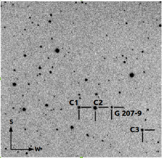
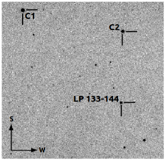
Figure 2: CCD frames with the variable and comparison stars marked. The field of view is $\approx 7\arcmin\times 7\arcmin$.

3.1 G 207-9

3.1.1 Previous observations

G 207-9 was announced as the 8th known member of pulsating white dwarf stars in 1976 (Robinson & McGraw, 1976). Four high ($\mathrm{F}_{1}$–$\mathrm{F}_{4}$) and one low ($\mathrm{F}_{5}$) amplitude peaks were detected at $\mathrm{F}_{1}=1354$, $\mathrm{F}_{2}=1794$, $\mathrm{F}_{3}=3145$, $\mathrm{F}_{4}=3425$ and $\mathrm{F}_{5}=3860\,\mu$Hz. Even though G 207-9 is a relatively bright target, and has been known as a pulsator for decades, no other time series photometric observations and frequency analysis have been published on this star up to now.

3.1.2 Konkoly observations

The analyses of the daily datasets revealed one dominant and four low amplitude peaks in the FTs. The dominant frequency of all nights’ observations in 2007 was at $3426\,\mu$Hz. This was the 3rd highest amplitude mode in 1975 ($\mathrm{F}_{4}=3425\,\mu$Hz). Two lower amplitude frequencies at $1672$ and $5098\,\mu$Hz reached the 4 S/N detection limit in 12 and 14 of the daily datasets, respectively. Two additional low-amplitude frequencies were detected at $1608$ and $7725\,\mu$Hz in 3 and 4 cases, respectively. These frequencies are medians of the daily values. The $1608$ and $1672\,\mu$Hz frequencies could be determined separately only in the last three nights’ datasets. We present the FT of one night’s dataset (the second longest run) in the first panel of Fig. 3.

Considering the consecutive nights of observations, five weekly time base datasets can be formed: Week 1 (JD 2 454 185–193), Week 2 (JD 2 454 267–272), Week 3 (JD 2 454 288–292), Week 4 (JD 2 454 308–314) and Week 5 (JD 2 454 323–328). The Fourier analyses of these data verified the five frequencies found by the daily observations. In three cases the first harmonic of the dominant frequency was also detected. Additionally, the analysis of the Week 2 and Week 5 data suggested that the peaks at $\sim 1672$ and $\sim 5098\,\mu$Hz may be actually doublets or triplets and not singlet frequencies. The separations of the frequency components were found to be between $\sim 2$ (close to the resolution limit) and $14\,\mu$Hz, but we mark these findings uncertain because of the effect of the 1 d^-1 aliasing. The 2nd–6th panels of Fig. 3 shows the FTs of the weekly datasets. We found only slight amplitude variations from one week to another. The amplitude of the dominant frequency varied between 8.6 and 10.5 mmag.

Figure 3: G 207-9: amplitude spectra of one night’s observation (top panel) and the weekly datasets (lower panels).

The standard pre-whitening of the whole dataset resulted 26 frequencies above the 4 S/N limit. Most of them are clustering around the frequencies already known by the analyses of the daily and weekly datasets. Generally, amplitude and (or) phase variations during the observations can be responsible for the emergence of such closely spaced peaks. In such cases, these features are just artefacts in the FT, as we fit the light curve with fixed amplitudes and frequencies during the standard pre-whitening process. Another possibility is that some of the closely spaced peaks are rotationally split frequencies. We can resolve such frequencies if the time base of the observations is long enough. The Rayleigh frequency resolution ($1/\Delta T$) of the whole dataset is $0.08\,\mu$Hz. We also have to consider the 1 d^-1 alias problem of single-site observations, which results uncertainties in the frequency determination.

Table 3: G 207-9: frequency content of the 2007 dataset. The errors were calculated by Monte Carlo simulations. $\delta f$ denotes the frequency differences of the closely spaced frequencies to $f_{1}$, $f_{2}$ or $f_{4}$.

	Frequency	Period	$\lvert\delta f\rvert$	Ampl.	S/N
				$\pm 0.1$
	($\mu$Hz)	(s)	($\mu$Hz)	(mmag)
$f_{1}$	$3426.303\pm 0.001$	291.9		10.1	111.5
$f_{2}$	$1678.633\pm 0.003$	595.7		2.0	15.4
$f_{1}^{-}?$	$3414.639\pm 0.004$	292.9	11.7	1.6	18.0
$f_{3}$	$5098.861\pm 0.003$	196.1		1.2	12.5
$f_{2}^{-}?$	$1667.328\pm 0.005$	599.8	11.3	1.1	8.6
$f_{4}$	$1603.071\pm 0.004$	623.8		1.1	8.1
$f_{1}^{+}?$	$3437.384\pm 0.005$	290.9	11.1	1.0	11.6
$f_{5}$	$7726.540\pm 0.003$	129.4		1.0	13.0
$f_{4}^{-}?$	$1595.481\pm 0.004$	626.8	7.6	0.8	6.1
$2f_{1}$	$6852.604\pm 0.005$	145.9		0.6	8.5
$f_{6}$	$3146.670\pm 0.007$	317.8		0.5	5.0
$f_{7}$	$3276.485\pm 0.008$	305.2		0.4	4.6

Figure 4: G 207-9: FT of the whole dataset, the window function is given in the inset (top panel). We emphasized the frequency domains of $f_{1}-f_{7}$ and $2f_{1}$, as seen in the original FT or during the pre-whitening process (lower panels).

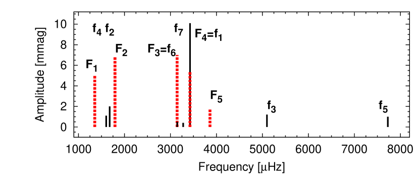
Figure 5: G 207-9: comparison of the frequencies obtained in 1975 (red dashed lines) and in 2007 (black solid lines). The amplitudes of the 1975 observations are from the paper of Mukadam et al. (2006).

We checked the frequency content of the whole dataset by averaging three consecutive data points of the $10\,$s measurements as a test. That is, we created a new, more homogeneous dataset mimicking $30\,$s exposure times. We then compared the frequency solutions of this $30\,$s dataset with the frequencies of the original mixed $10$–$30\,$s data. Finally, we accepted as the frequencies characterizing the whole light curve the frequencies that could be determined in both datasets, that is, without 1 d^-1 differences. This resulted a reduced frequency list of 12 frequencies. We list them in Table 3. There are still several closely spaced frequencies around three of the main frequencies ($f_{1}$, $f_{2}$ and $f_{4}$) remained with separations between $7.6$ and $11.7\,\mu$Hz. In the case of $f_{1}$ and $f_{2}$, these separations are close to $11.574\,\mu$Hz (1 d^-1). It is possible that at least some of these frequency components are results of rotational splitting, but considering the uncertainties mentioned above, we do not accept them as rotationally split frequencies. In such cases when the frequency separations of the rotationally split components are around 1 d^-1, multi-site or space-based observations are needed for reliable determination of the star’s rotational rate.

Summing it up: besides the five frequencies ($f_{1}$–$f_{5}$) known also by the analyses of shorter (daily and weekly) data segments, we could detect two additional independent frequencies ($f_{6}$ and $f_{7}$) in the whole dataset. Frequency $f_{6}$ at $3146.7\,\mu$Hz was also detected in 1975 ($\mathrm{F}_{3}=3145\,\mu$Hz). Moreover, this was one of the dominant peaks at that time. Frequency $f_{7}$ at $3276.5\,\mu$Hz is a newly detected one. Note that the frequency $f_{7}$ is close to $f_{2}+f_{4}=3281.7\,\mu$Hz, however, the difference is $5.2\,\mu$Hz, which seems too large to claim that $f_{7}$ is the linear combination of these peaks considering the errors. Thus, we consider $f_{7}$ as an independent mode. Fig. 4 shows the FT of the whole dataset and the frequency domains of $f_{1}-f_{7}$ on separate panels.

Comparing the frequency content of the 1975 and 2007 observations, we can conclude that three of the five frequencies found in the 1975 dataset did not appear in 2007 ($\mathrm{F}_{1}$, $\mathrm{F}_{2}$ and $\mathrm{F}_{5}$), while two stayed at an observable level ($\mathrm{F}_{3}=f_{6}$ and $\mathrm{F}_{4}=f_{1}$). Figure 5 summarizes the frequencies of the two epochs. It seems that even though there were no large amplitude variations during our five-months observing season in 2007, on the time scale of years or decades, remarkable changes can happen in the pulsation of G 207-9: new frequencies can be excited to a significant level, while other modes can disappear.

3.2 LP 133-144

3.2.1 Previous observations

The variability of LP 133-144 was discovered in 2003 (Bergeron et al., 2004). Four pulsation frequencies were determined at that time, including two closely spaced peaks: $\mathrm{F}_{1}=3055.1$, $\mathrm{F}_{2}=3258.4$, $\mathrm{F}_{3}=3284.1$ and $\mathrm{F}_{4}=4780.6\,\mu$Hz. Similarly to the case of G 207-9, no further results of time series photometric observations have been published up to now.

3.2.2 Konkoly observations

We found four recurring frequencies in the daily datasets at 3055, 3270, 3695 and 4780 $\mu$Hz (median values). Their amplitudes varied from night to night, but the 4780 $\mu$Hz peak was the dominant in almost all cases. One additional peak exceeded the 4 S/N limit at 5573 $\mu$Hz, but on one night only.

We created four monthly datasets and analysed them independently. These are Month 1 (JD 2 454 115–130), Month 2 (JD 2 454 175–194), Month 3 (JD 2 454 203–208) and Month 4 (JD 2 454 231–237). The analyses of the monthly data revealed that at the 3270, 3695 and 4780 $\mu$Hz frequencies there are actually doublets or triplets with 2.6–4.7 $\mu$Hz frequency separations. This explains the different amplitudes in the daily FTs. The 3055 $\mu$Hz frequency was found to be a singlet. In Month 3, the linear combination of the largest amplitude components of the 3270 and 4780 $\mu$Hz multiplets also could be detected. The 5573 $\mu$Hz frequency was significant in Month 2.

The panels of Fig. 6 show the FT of one daily dataset and the monthly data. As in the case of G 207-9, there were no remarkable amplitude variations from one month to another.

Figure 6: LP 133-144: amplitude spectra of one night’s observation (top panel) and the monthly datasets (lower panels).

The analysis of the whole 2007 dataset resulted in the detection of 19 significant frequencies in the $\sim 2300-8000\,\mu$Hz frequency region. We also performed the test analysis utilizing the averaged 30 s dataset, which confirmed the presence of the 14 largest amplitude frequencies (the other five peaks remained slightly under the significance level). Thus we accepted them as the frequencies characterizing the pulsation of LP 133-144 and list them in Table 4. The Rayleigh frequency resolution of the whole dataset is $0.09\,\mu$Hz.

Table 4: LP 133-144: frequency content of the 2007 dataset. The errors were calculated by Monte Carlo simulations. $\delta f$ denotes the frequency differences of the closely spaced frequencies to $f_{1}$, $f_{2}$ $f_{3}$ or $f_{6}$. We discuss the case of $f_{6}$ in the text. The signal-to-noise ratios refer to the original 10-30 s dataset.

	Frequency	Period	$\lvert\delta f\rvert$	Ampl.	S/N
				$\pm 0.1$
	($\mu$Hz)	(s)	($\mu$Hz)	(mmag)
$f_{1}$	4780.555$\pm$0.001	209.2		10.9	100.9
$f_{2}$	3269.302$\pm$0.001	305.9		3.9	35.4
$f_{3}$	3695.083$\pm$0.002	270.6		3.5	31.2
$f_{3}^{-}$	3691.627$\pm$0.002	270.9	3.5	3.4	30.5
$f_{2}^{+}$	3272.475$\pm$0.002	305.6	3.2	3.0	26.7
$f_{4}$	3055.125$\pm$0.002	327.3		2.8	25.1
$f_{3}^{+}$	3698.551$\pm$0.003	270.4	3.5	2.0	18.4
$f_{2}^{-}$	3266.125$\pm$0.005	306.2	3.2	1.2	10.4
$f_{1}^{+}$	4784.696$\pm$0.005	209.0	4.1	1.1	10.6
$f_{1}^{-}$	4776.400$\pm$0.007	209.4	4.2	1.0	8.7
$f_{5}$	7116.986$\pm$0.010	140.5		0.6	5.9
$f_{6}^{+}$	5574.381$\pm$0.009	179.4	4.8	0.6	6.0
$2f_{1}$	9561.115$\pm$0.011	104.6		0.5	5.5
$f_{6}^{-}$	5564.876$\pm$0.013	179.7	4.7	0.5	5.1
($f_{6}$)	5569.618$\pm$0.020	179.5		0.4	4.1

The first eleven peaks in Table 4 are three triplets with frequency separations of $4.1-4.2\,\mu$Hz ($f_{1}$), $3.2\,\mu$Hz ($f_{2}$) or $3.5\,\mu$Hz ($f_{3}$), and two singlet frequencies ($f_{4}$ and $f_{5}$). In the case of $f_{6}$, three peaks can be determined in the original 10-30 s dataset with frequency separations of $4.7-4.8\,\mu$Hz. However, the low amplitude central peak of this triplet at $f_{6}=5569.6\,\mu$Hz do not reach the 4 S/N significance limit in the test 30 s data. Still, to make the discussion of the triplet structures clear, we added $f_{6}$ to the list of Table 4 in parentheses. Besides these, the first harmonic of $f_{1}$ also appeared. Fig. 7 shows the FT of the whole dataset, the consecutive pre-whitening steps at the multiplet frequencies and at the frequency domains of $f_{4}$, $f_{5}$ and $2f_{1}$.

We plot the frequencies of Bergeron et al. (2004) and the frequencies found in the 2007 Konkoly observations together in Fig. 8. Assuming that the closely spaced peaks at $\mathrm{F}_{2}$ and $\mathrm{F}_{3}$ are results of the not properly resolved components of the $f_{2}$ triplet, we found, with similar amplitudes, all the frequencies observed in 2003. Besides these, we detected three new frequencies: a relatively large amplitude mode at $f_{3}$, and two additional low-amplitude modes at $f_{5}$ and $f_{6}$. That is, we doubled the number of modes can be used for the asteroseismic fits.

The schematic plot of the triplets can be seen in Fig. 9. It is clearly visible that the frequency separations of the components are larger at higher frequencies. We discuss the rotation of LP 133-144 based on the investigation of these triplets in Sect. 4.3.1.

Figure 7: LP 133-144: FT of the whole dataset, the window function is given in the inset (top panel). We also plotted the FTs of the consecutive pre-whitening steps at the multiplet frequencies $f_{1}$, $f_{2}$, $f_{3}$ and $f_{6}$, the frequency domains of the singlets $f_{4}$ and $f_{5}$, and the peak at $2f_{1}$ (lower panels). The bottom panels show the residual spectra after pre-whitening with the denoted frequencies.

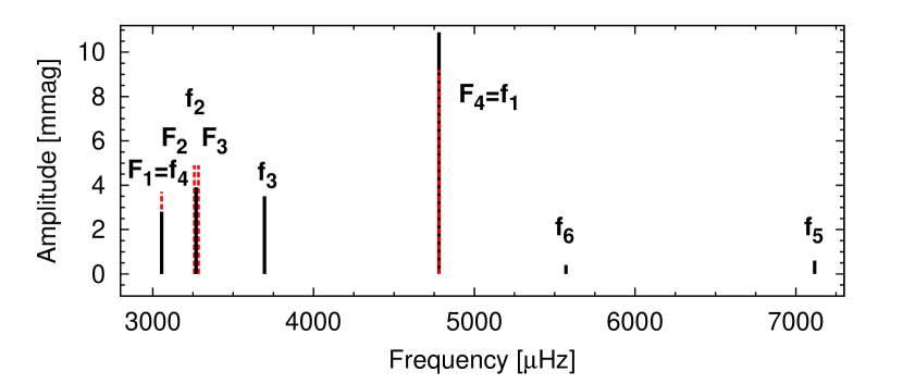
Figure 8: LP 133-144: comparison of the frequencies obtained in 2003 (red dashed lines) and in 2007 (black solid lines).

Figure 9: LP 133-144: schematic plot of the triplets found at different frequency domains. The frequency errors are comparable to the width of the lines.

4 Asteroseismology

We built our model grid for the asteroseismic investigations of our targets utilizing the White Dwarf Evolution Code (wdec; Lamb 1974; Kutter & Savedoff 1969; Lamb & van Horn 1975; Winget 1981; Kawaler 1986; Wood 1990; Bradley 1993; Montgomery 1998; Bischoff-Kim et al. 2008). The wdec evolves a hot polytrope model ($\sim 10^{5}$ K) down to the requested temperature, and provides an equilibrium, thermally relaxed solution to the stellar structure equations. Then we are able to calculate the set of possible zonal ($m=0$) pulsation modes according to the adiabatic equations of non-radial stellar oscillations (Unno et al., 1989). We utilized the integrated evolution/pulsation form of the wdec code created by Metcalfe (2001) to derive the pulsation periods for the models with the given stellar parameters. More details on the physics applied in the wdec can be found with references in Bischoff-Kim et al. (2008) and in our previous papers on two ZZ Ceti stars (Bognár et al., 2009; Paparó et al., 2013).

Considering the limited visibility of high spherical degree ($l$) modes due to geometric cancellation effects, we calculated the periods of dipole ($l=1$) and quadrupole ($l=2$) modes for the model stars only. The goodness of the fit between the observed ($P_{i}^{\mathrm{obs}}$) and calculated ($P_{i}^{\mathrm{calc}}$) periods was characterized by the root mean square ($\sigma_{\mathrm{{rms}}}$) value calculated for every model with the fitper program of Kim (2007):

$$\sigma_{\mathrm{{rms}}}=\sqrt{\frac{\sum_{i=1}^{N}(P_{i}^{\mathrm{calc}}-P_{i}^{\mathrm{obs}})^{2}}{N}}$$ (1)

where N is the number of observed periods.

We varied five main stellar parameters to build our model grid: the effective temperature ($T_{\mathrm{eff}}$), the stellar mass ($M_{*}$), the mass of the hydrogen layer ($M_{\mathrm{H}}$), the central oxygen abundance ($X_{\mathrm{O}}$) and the fractional mass point where the oxygen abundance starts dropping ($X_{\mathrm{fm}}$). We fixed the mass of the helium layer ($M_{\mathrm{He}}$) at $10^{-2}\,M_{*}$. The grid covers the parameter range $11\,400-12\,800$ K in $T_{\mathrm{eff}}$ (the middle and hot part of the ZZ Ceti instability strip), $0.500-0.900\,M_{\sun}$ in stellar mass, $10^{-4}-10^{-8}\,M_{*}$ in $M_{\mathrm{H}}$, $0.3-0.9$ in $X_{\mathrm{O}}$ and $0.1-0.7$ in $X_{\mathrm{fm}}$. We used step sizes of $200$ K ($T_{\mathrm{eff}}$), $0.005\,M_{\sun}$ ($M_{*}$), $0.2$ dex (log $M_{\mathrm{H}}$) and 0.1 ($X_{\mathrm{O}}$ and $X_{\mathrm{fm}}$).

4.1 Period lists

In the case of G 207-9, we could detect seven linearly independent pulsation frequencies by the 2007 Konkoly dataset ($f_{1}-f_{7}$; see Table 3). The question is, if we could add more frequencies to this list by the 1975 observations of Robinson & McGraw (1976). As we mentioned already in Sect. 3.1.2, two of the frequencies detected in 1975 were also found in the Konkoly data ($\mathrm{F}_{3}=f_{6}$ and $\mathrm{F}_{4}=f_{1}$). The status of the remaining three 1975 frequencies is questionable. Assuming at least a couple of $\mu$Hz errors for the 1975 frequencies, $\mathrm{F}_{1}=\mathrm{F}_{3}-\mathrm{F}_{2}$ (or $\mathrm{F}_{2}=\mathrm{F}_{3}-\mathrm{F}_{1}$, or $\mathrm{F}_{3}=\mathrm{F}_{1}+\mathrm{F}_{2}$), thus, these three frequencies do not seem to be linearly independent. The fact that $\mathrm{F}_{2}$ and $\mathrm{F}_{3}$ are the two dominant peaks in the FT of Robinson & McGraw (1976) suggests that $\mathrm{F}_{2}$ and $\mathrm{F}_{3}$ might be the parent modes and $\mathrm{F}_{1}$ is a combination peak. Furthermore, Robinson & McGraw (1976) pointed out that $\mathrm{F}_{5}-\mathrm{F}_{4}\approx\mathrm{F}_{2}-\mathrm{F}_{1}$, thus, further combinations are possible. We also note that $f_{5}$ of the Konkoly dataset is almost at twice the value of $\mathrm{F}_{5}$ ($\delta f=6.5\mu$Hz), however, there is no sign of any pulsation frequency at $0.5f_{5}$ in the 2007 data.

We used two sets of observed periods to fit the calculated ones. One set consists of the seven periods of $f_{1}-f_{7}$ observed in 2007, while we complemented this list with the period of $\mathrm{F}_{2}$ detected in 1975 to create another set. We selected $\mathrm{F}_{2}$ because it was the second largest amplitude peak in 1975, which makes it a good candidate for an additional normal mode.

In LP 133-144, we found all the previously observed frequencies in our 2007 dataset, as we show in Sect. 3.2.2. Thus, we cannot add more frequencies to our findings, and performed the model fits with six periods. We summarized the periods utilized for modelling in Table 5 for both stars.

Table 5: G 207-9 and LP 133-144: periods utilized for the model fits.

G 207-9		LP 133-144
	Period		Period
	(s)		(s)
$f_{1}$	291.9	$f_{1}$	209.2
$f_{2}$	595.7	$f_{2}$	305.9
$f_{3}$	196.1	$f_{3}$	270.6
$f_{4}$	623.8	$f_{4}$	327.3
$f_{5}$	129.4	$f_{5}$	140.5
$f_{6}$	317.8	$f_{6}$	179.5
$f_{7}$	305.2
+$\mathrm{F}_{2}$	557.4

4.2 Best-fitting models for G 207-9

We determined the best-matching models considering several cases: at first, we let all modes to be either $l=1$ or $l=2$. Then we assumed that the dominant peak is an $l=1$, considering the better visibility of $l=1$ modes over $l=2$ ones. At last, we searched for the best-fitting models assuming that at least four of the modes is $l=1$, including the dominant frequency.

We obtained the same model as the best-fitting asteroseismic solution both for the seven- and eight-period fits. It has $T_{\mathrm{eff}}=12\,000$ K, $M_{*}=0.870\,M_{\sun}$ and $M_{\mathrm{H}}=10^{-4}\,M_{*}$. This model has the lowest $\sigma_{\mathrm{{rms}}}$ ($1.04-1.06$ s) both if we do not apply any restrictions on the $l$ values of the modes, and as it gives $l=1$ solution to the dominant frequency, this model is also the best-fit if we assume that the $291.9$ s mode is $l=1$. Note that in this model solution only this mode is an $l=1$, all the other six or seven modes are $l=2$.

In the case of four expected $l=1$ modes and seven periods, the best-matching model has the same effective temperature ($T_{\mathrm{eff}}=12\,000$ K), a bit lower stellar mass ($M_{*}=0.865\,M_{\sun}$), and thinner hydrogen layer ($M_{\mathrm{H}}=10^{-6}\,M_{*}$). Assuming four $l=1$ modes and eight periods, the best-matching model has $T_{\mathrm{eff}}=12\,400$ K, $M_{*}=0.855\,M_{\sun}$ and $M_{\mathrm{H}}=10^{-4.6}\,M_{*}$. The second best-fit model is the same as for four $l=1$ modes and seven periods. We denoted with open circles these two latter models in Fig. 10 (left panel) on the $T_{\mathrm{eff}}-M_{*}$ plane, together with the spectroscopic solution. Both in the case of G 207-9 and LP 133-144, we utilized the $T_{\mathrm{eff}}$ and surface gravity ($\mathrm{log}\,g$) values provided by Gianninas et al. (2011), and then corrected them according to the results of Tremblay et al. (2013) based on radiation-hydrodynamics 3D simulations of convective DA stellar atmospheres. We accepted the resulting values as the best estimates for these atmospheric parameters. We converted the surface gravities to stellar masses utilizing the theoretical masses determined for DA stars by Bradley (1996).

Considering the mass of the hydrogen layer (see the left panel of Fig. 11), we found that most of the models up to $\sigma_{\mathrm{{rms}}}=3.0$ s are in the $M_{\mathrm{H}}=10^{-4}-10^{-6}\,M_{*}$ range, while about a dozen models predict thinner hydrogen layer down to $10^{-8}\,M_{*}$. The best-fitting models favour the $M_{\mathrm{H}}=10^{-4.6}\,M_{*}$ value.

We summarize the results of the spectroscopic atmospheric parameter determinations, the former modelling results based on the 1975 frequency list, the main stellar parameters of the models mentioned above and the calculated periods fitted with our observed ones in Table 6. We also list the $\sigma_{\mathrm{{rms}}}$ values of the models. The $T_{\mathrm{eff}}=12\,000$ K solutions are in agreement with the spectroscopic value. The $T_{\mathrm{eff}}=12\,400$ K model seems somewhat too hot comparing to the $\sim 12\,100$ K spectroscopic temperature, but considering that the uncertainties of both values are estimated to be around $200$ K, this model still not contradicts to the observations. The $0.855-0.870\,M_{*}$ stellar masses are also close to the value derived by spectroscopy, considering its uncertainty. Summing it up, we can find models with stellar parameters and periods close to the observed values even if we assume that at least half of the modes is $l=1$, including the dominant mode.

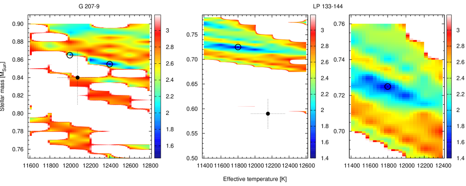
Figure 10: Models on the $T_{\mathrm{eff}}-M_{*}$ plane with their $\sigma_{\mathrm{{rms}}}$ values (colour coded). Left panel: G 207-9; models fitting with eight periods and assuming that at least half of the modes is $l=1$, including the dominant mode. The two models with the lowest $\sigma_{\mathrm{{rms}}}$ values (for more explanation, see the text) are denoted with open circles. Black dot marks the spectroscopic value (cf. Table 6). Middle panel: LP 133-144; models fitting with six periods and assuming that the three largest amplitude modes (also showing triplets) are $l=1$. The best-fitting model is denoted with an open circle, the spectroscopic value presented in Table 7 is signed with a black dot. Right panel: magnified part of the middle panel’s plot around the best-matching model. We used interpolation in the plots for better visibility.

Figure 11: Mass of the hydrogen layer of models at different $\sigma_{\mathrm{{rms}}}$ values. Left panel: G 207-9, right panel: LP 133-144. We plotted the same models that are presented in Fig. 10.

Table 6: G 207-9: results on the main stellar parameters obtained by spectroscopic observations (‘Spectroscopy’), previous model fits (‘Modelling’) and modelling presented in this paper (‘This work’). In the ‘Modelling’ part, we listed the observed periods used for the fits. In the case of our model fits, we listed the observed periods first and present the theoretical periods at the actual models. The $\sigma_{\mathrm{{rms}}}$ values are given at the effective temperatures in parentheses. In the case of model fits the identification of pulsation modes - spherical degree ($l$) and radial order ($k$) values - are also presented.

$T_{\mathrm{eff}}$ (K)	$M_{*}/M_{\sun}$	-log $M_{\mathrm{He}}$	-log $M_{\mathrm{H}}$	Periods in seconds ($l$, $k$)	Reference
Spectroscopy:
12 078$\pm$200	0.84$\pm$0.03				Gianninas et al. (2011)
					Tremblay et al. (2013)
Modelling:
12 000	0.815	2.0	8.5	259.0, 292.0, 317.3, 557.3, 740.7, 787.5⋆	Castanheira & Kepler (2009)
11 700	0.530	3.5	6.5	259.0, 292.0, 317.3, 557.3, 740.7, 787.5⋆	Castanheira & Kepler (2009)
12 030	0.837	2.5	6–7	259.1 (1,4), 292.0 (2,10), 318.0 (1,5),	Romero et al. (2012); Romero et al. (2013)
				557.4 (1,12), 740.4 (1,17)
This work:				291.9, 595.7, 196.1, 623.8, 129.4, 317.8, 305.2, 557.4
12 000 (1.06 s)	0.870	2.0	4.0	291.0 (1,7), 595.5 (2,32), 195.8 (2,9),
				625.6 (2,34), 129.0 (2,5), 319.7 (2,16),
				305.4 (2,13), 558.6 (2,28)
12 000 (1.61 s)	0.865	2.0	6.0	290.6 (1,5), 594.5 (1,14), 193.1 (2,6),
				623.9 (1,15), 130.4 (2,3), 316.6 (1,6),
				306.2 (2,12), 555.1 (2,24)
12 400 (1.50 s)	0.855	2.0	4.6	290.5 (1,6), 594.7 (1,16), 194.0 (1,3),
				624.7 (1,17), 132.3 (2,4), 318.7 (2,14),
				304.6 (2,13), 557.0 (2,27)
⋆ The utilized periods were mean values of the periods of Robinson & McGraw (1976) and the periods of WD J0815+4437 showing
similar pulsation modes.

4.3 Best-fitting models for LP 133-144

The model with the lowest $\sigma_{\mathrm{{rms}}}$ ($0.46$ s) has $T_{\mathrm{eff}}=11\,800$ K, $M_{*}=0.710\,M_{\sun}$ and $M_{\mathrm{H}}=10^{-4.0}\,M_{*}$ if we do not apply any restrictions on the $l$ values of modes. Generally, the best-matching models have masses around $0.7\,M_{\sun}$, which are at least $0.1\,M_{\sun}$ larger than the spectroscopic value. These models provide $3-4$ $l=1$ solutions to the observed modes.

We searched for the best-matching models in a second run, assuming that the three largest amplitude modes showing triplet structures at 209.2, 305.9 and 270.6 s are all $l=1$ modes. The best-matching model has the same effective temperature ($T_{\mathrm{eff}}=11\,800$ K), slightly larger mass ($M_{*}=0.725\,M_{\sun}$) and much thinner hydrogen layer ($M_{\mathrm{H}}=10^{-8.0}\,M_{*}$) than the previously selected model. The mass still seems too large comparing to the spectroscopic value, but it gives $l=1$ solutions for all the four modes with triplet frequencies, including the mode at 179.5 s. These modes are consecutive radial overtones with $k=1-4$. We denoted this model with an open circle on the middle and right panels of Fig. 10. The hydrogen layer masses versus the $\sigma_{\mathrm{{rms}}}$ values of these models are plotted in the right panel of Fig. 11. This figure also shows that the best-fitting models have thin hydrogen layer with $M_{\mathrm{H}}=10^{-8.0}\,M_{*}$. Otherwise, two families of model solutions outlines: one with $M_{\mathrm{H}}=10^{-4.0}-10^{-6.0}\,M_{*}$ and one with thinner, $M_{\mathrm{H}}=10^{-7.6}-10^{-8.0}\,M_{*}$ hydrogen layers.

If we restrict our period fitting to the models with effective temperatures and masses being in the range determined by spectroscopy, the best-matching model has $T_{\mathrm{eff}}=12\,000$ K, $M_{*}=0.605\,M_{\sun}$ and $M_{\mathrm{H}}=10^{-4.2}\,M_{*}$. However, the 179.5 s mode is $l=2$ in this case, while all the other frequencies are consecutive radial order $l=1$ modes.

At last, we searched for models in this restricted parameter space and assuming that all the four frequencies showing triplets are $l=1$. Our finding with the lowest $\sigma_{\mathrm{{rms}}}$ has $T_{\mathrm{eff}}=12\,000$ K, $M_{*}=0.585\,M_{\sun}$ and $M_{\mathrm{H}}=10^{-5.0}\,M_{*}$, however, its $\sigma_{\mathrm{{rms}}}$ is relatively large ($6.8$ s), which means that there are major differences between the observed and calculated periods. Table 7 lists the stellar parameters and theoretical periods of the models mentioned above. For completeness, we included this last model solution, too.

We concluded, that our models predict at least $0.1\,M_{\sun}$ larger stellar mass for LP 133-144 than the spectroscopic value. Nevertheless, it is possible to find models with lower stellar masses, but in these cases not all the modes with triplet frequency structures has $l=1$ solutions and (or) the corresponding $\sigma_{\mathrm{{rms}}}$ values are larger than for the larger mass models. Considering the effective temperatures, the $T_{\mathrm{eff}}=12\,000$ K solutions are in agreement with the spectroscopic determination ($\sim 12\,150$ K) within its margin of error. As in the case of G 207-9, taking into account that the uncertainties for the grid parameters are of the order of the step sizes in the grid, the $T_{\mathrm{eff}}=11\,800$ K findings are still acceptable.

Table 7: Same as in Table 6 but for LP 133-144.

$T_{\mathrm{eff}}$ (K)	$M_{*}/M_{\sun}$	-log $M_{\mathrm{He}}$	-log $M_{\mathrm{H}}$	Periods in seconds ($l$, $k$)	Reference
Spectroscopy:
12 152$\pm$200	0.59$\pm$0.03				Gianninas et al. (2011)
					Tremblay et al. (2013)
Modelling:
11 700	0.520	2.0	5.0	209.2 (1,2), 305.7 (2,7), 327.3 (2,8)	Castanheira & Kepler (2009)
12 210	0.609	1.6	$\sim 6$	209.2 (1,2), 305.7 (2,8), 327.3 (2,9)	Romero et al. (2012)
This work:				209.2, 305.9, 270.6, 327.3, 140.5, 179.5
11 800 (0.46 s)	0.710	2.0	4.0	208.8 (1,3), 305.6 (2,11), 270.1 (1,5),
				327.2 (1,6), 140.6 (2,4), 180.4 (1,2)
11 800 (1.46 s)	0.725	2.0	8.0	209.5 (1,2), 304.5 (1,4), 268.8 (1,3),
				328.3 (2,9), 138.5 (2,2), 181.0 (1,1)
12 000 (2.89 s)	0.605	2.0	4.2	204.5 (1,2), 307.9 (1,4), 271.5 (1,3),
				326.2 (1,5), 138.4 (1,1), 183.7 (2,4)
12 000 (6.83 s)	0.585	2.0	5.0	215.3 (1,2), 311.6 (1,4), 273.3 (1,3),
				326.6 (2,9), 126.6 (2,2), 176.4 (1,1)

4.3.1 Stellar rotation

A plausible explanation for the observed triplet structures is that these are rotationally split frequency components of $l=1$ modes. We used this assumption previously in searching for model solutions for our observed periods. Knowing the frequency differences of the triplet components ($\delta f$), we can estimate the rotation period of the pulsator.

In the case of slow rotation, the frequency differences of the $m=-1,0,1$ rotationally split components can be calculated (to first order) by the following relation:

$$\delta f_{k,\ell,m}=\delta m(1-C_{k,\ell})\Omega,$$ (2)

where the coefficient $C_{k,\ell}\approx 1/\ell(\ell+1)$ for high-overtone ($k\gg\ell$) $g$-modes and $\Omega$ is the (uniform) rotation frequency.

In the case of LP 133-144, the presumed $l=1$ modes are low radial-order frequencies ($k=1-6$), but the $C_{k,\ell}$ values of the fitted modes can be derived by the asteroseismic models. We used the average of the frequency separations within a triplet and calculated the stellar rotation rate separately for $f_{1}$, $f_{2}$, $f_{3}$ and $f_{6}$ (see e.g. Hermes et al. 2015a). We utilized the $T_{\mathrm{eff}}=11\,800$ K, $M_{*}=0.725\,M_{\sun}$ model. The resulting rotation periods are: $P_{f_{1}}=1.83$ d ($\overline{\delta f_{1}}=4.15\,\mu$Hz, $C_{k,\ell}=0.345$), $P_{f_{2}}=1.82$ d ($\overline{\delta f_{2}}=3.2\,\mu$Hz, $C_{k,\ell}=0.497$), $P_{f_{3}}=1.69$ d ($\overline{\delta f_{3}}=3.5\,\mu$Hz, $C_{k,\ell}=0.489$) and $P_{f_{6}}=1.60$ d ($\overline{\delta f_{6}}=4.75\,\mu$Hz, $C_{k,\ell}=0.343$). The average rotation period thus $1.74\pm 0.11$ d ($\sim 42$ h). This fits perfectly in the known rotation rates of the order of hours to days of ZZ Ceti stars (cf. Table 4 in Fontaine & Brassard 2008). Note that the rotation periods calculated by the different multiplet structures are strongly depend on the actual values of observed frequency spacings and also on the $C_{k,\ell}$ values, which vary from model to model. Thus the different rotation periods calculated for the different modes does not of necessarily mean that e.g. in this case we detected differential rotation of the star, but we can provide a reasonable estimation on the global rotation period of LP 133-144.

5 Summary and Conclusions

We have presented the results of the one-season-long photometric observations of the ZZ Ceti stars G 207-9 and LP 133-144. These rarely observed pulsators are located in the middle and in the hot part of the instability strip, respectively. G 207-9 was found to be a massive object previously by spectroscopic observations, comparing its predicted $M_{*}>0.8\,M_{\sun}$ mass to the average $\sim 0.6\,M_{\sun}$ value of DA stars (see e.g. Kleinman et al. 2013). In contrary, the mass of LP 133-144 was expected to be around this average value.

With our observations performed at Konkoly Observatory, we extended the number of known pulsation frequencies in both stars. We found seven linearly independent modes in G 207-9, including five newly detected frequencies, comparing to the literature data. We also detected the possible signs of additional frequencies around some of the G 207-9 modes, but their separations being close to the 1 d^-1 value makes their detection uncertain. Multi-site or space-based observations could verify or disprove their presence. In the case of LP 133-144, we detected three new normal modes out of the six derived, and revealed that at least at three modes there are actually triplet frequencies with frequency separations of $\sim 4\mu$Hz.

All the pulsation modes of LP 133-144 and most of the modes of G 207-9 are found to be below 330 s, with amplitudes up to $\sim 10$ mmag. This fits to the well-known trend observed at ZZ Ceti stars that at higher effective temperatures we see lower amplitude and shorter period light variations than closer to the red edge of the instability strip (see e.g. Fontaine & Brassard 2008). We also found that on the five-month time scale of our observations there were no significant amplitude variations in either stars. This suits to their location in the instability domain again, as short time scale large amplitude variations are characteristics of ZZ Cetis with lower effective temperatures. However, in the case of G 207-9, the different frequency content of the 1975 and 2007 observations shows that amplitude variations do occur on decade-long time scale.

In addition, similar pulsational feature of the two stars is that both show light variations with one dominant mode ($A=10-11$ mmag) and several lower amplitude frequencies.

The extended list of known modes allowed to perform new asteroseismic fits for both objects, in which we compared the observed and calculated periods both with and without any restrictions on the $l$ values of modes. The best-matching models of G 207-9 have found to be close to the spectroscopic effective temperature and stellar mass, predicting $T_{\mathrm{eff}}=12\,000$ or $12\,400$ K and $M_{*}=0.855-0.870\,M_{\sun}$. For LP 133-144, the best-fitting models prefer more than $0.1\,M_{\sun}$ larger stellar masses than the spectroscopic measurements and $T_{\mathrm{eff}}=11\,800$ K effective temperatures. The main sources of the differences in our model solutions and the models presented by Castanheira & Kepler (2009), even though they also used the wdec, can arise from the different periods utilized for the fits, the different core composition profiles applied, and the different way they determined the best-fitting models utilizing the amplitudes of observed periods as weights to define the goodness of the fits. At last, we derived the rotational period of LP 133-144 based on the observed triplets and obtained $P_{\mathrm{rot}}\simeq 42$ h.

Note that the results of the asteroseismic fits presented in this manuscript are preliminary findings, and both objects deserve more detailed seismic investigations utilizing the extended period lists, similarly to the modelling presented for other hot DAV stars, GD 165 and Ross 548 (Giammichele et al., 2016). In the case of these objects, the authors could identify models reproducing the observed periods quite well while staying close to the spectroscopic stellar parameters, and also verified the credibility of the selected models in many other ways, including the investigation of rotationally split frequencies.

Appendix A

Normalized differential light curves of G 207-9 obtained in 2007 at Piszkéstető mountain station of Konkoly Observatory.

Appendix B

Normalized differential light curves of LP 133-144 obtained in 2007 at Piszkéstető mountain station of Konkoly Observatory.

References

- Althaus et al. (2010) Althaus L. G., Córsico A. H., Isern J., García-Berro E., 2010, A&ARv, 18, 471
- Bell et al. (2015) Bell K. J., Hermes J. J., Bischoff-Kim A., Moorhead S., Montgomery M. H., Østensen R., Castanheira B. G., Winget D. E., 2015, ApJ, 809, 14
- Bergeron et al. (2004) Bergeron P., Fontaine G., Billères M., Boudreault S., Green E. M., 2004, ApJ, 600, 404
- Bischoff-Kim (2009) Bischoff-Kim A., 2009, in Guzik J. A., Bradley P. A., eds, American Institute of Physics Conference Series Vol. 1170, American Institute of Physics Conference Series. pp 621–624, doi:10.1063/1.3246573
- Bischoff-Kim et al. (2008) Bischoff-Kim A., Montgomery M. H., Winget D. E., 2008, ApJ, 675, 1512
- Bognár et al. (2009) Bognár Z., Paparó M., Bradley P. A., Bischoff-Kim A., 2009, MNRAS, 399, 1954
- Bognár et al. (2014) Bognár Z., Paparó M., Córsico A. H., Kepler S. O., Győrffy Á., 2014, A&A, 570, A116
- Bognár et al. (2015) Bognár Z., Paparó M., Molnár L., Plachy E., Sódor Á., 2015, in Dufour P., Bergeron P., Fontaine G., eds, Astronomical Society of the Pacific Conference Series Vol. 493, 19th European Workshop on White Dwarfs. p. 245 (arXiv:1506.06960)
- Bradley (1993) Bradley P. A., 1993, PhD thesis, Texas Univ., Austin.
- Bradley (1996) Bradley P. A., 1996, ApJ, 468, 350
- Brickhill (1991) Brickhill A. J., 1991, MNRAS, 251, 673
- Castanheira & Kepler (2009) Castanheira B. G., Kepler S. O., 2009, MNRAS, 396, 1709
- Eastman et al. (2010) Eastman J., Siverd R., Gaudi B. S., 2010, PASP, 122, 935
- Fontaine & Brassard (2008) Fontaine G., Brassard P., 2008, PASP, 120, 1043
- Giammichele et al. (2016) Giammichele N., Fontaine G., Brassard P., Charpinet S., 2016, ApJS, 223, 10
- Gianninas et al. (2011) Gianninas A., Bergeron P., Ruiz M. T., 2011, ApJ, 743, 138
- Goldreich & Wu (1999) Goldreich P., Wu Y., 1999, ApJ, 511, 904
- Hermes et al. (2015a) Hermes J. J., et al., 2015a, MNRAS, 451, 1701
- Hermes et al. (2015b) Hermes J. J., et al., 2015b, ApJ, 810, L5
- Kawaler (1986) Kawaler S. D., 1986, PhD thesis, Texas Univ., Austin.
- Kepler et al. (1995) Kepler S. O., et al., 1995, ApJ, 447, 874
- Kim (2007) Kim A., 2007, PhD thesis, The University of Texas at Austin
- Kleinman et al. (2013) Kleinman S. J., et al., 2013, ApJS, 204, 5
- Kutter & Savedoff (1969) Kutter G. S., Savedoff M. P., 1969, ApJ, 156, 1021
- Lamb (1974) Lamb Jr. D. Q., 1974, PhD thesis, THE UNIVERSITY OF ROCHESTER.
- Lamb & van Horn (1975) Lamb D. Q., van Horn H. M., 1975, ApJ, 200, 306
- Metcalfe (2001) Metcalfe T. S., 2001, PhD thesis, The University of Texas at Austin
- Montgomery (1998) Montgomery M. H., 1998, PhD thesis, The University of Texas at Austin
- Mukadam et al. (2006) Mukadam A. S., Montgomery M. H., Winget D. E., Kepler S. O., Clemens J. C., 2006, ApJ, 640, 956
- Paparó et al. (2013) Paparó M., Bognár Z., Plachy E., Molnár L., Bradley P. A., 2013, MNRAS, 432, 598
- Robinson & McGraw (1976) Robinson E. L., McGraw J. T., 1976, ApJ, 207, L37
- Robinson et al. (1978) Robinson E. L., Stover R. J., Nather R. E., McGraw J. T., 1978, ApJ, 220, 614
- Romero et al. (2012) Romero A. D., Córsico A. H., Althaus L. G., Kepler S. O., Castanheira B. G., Miller Bertolami M. M., 2012, MNRAS, 420, 1462
- Romero et al. (2013) Romero A. D., Kepler S. O., Córsico A. H., Althaus L. G., Fraga L., 2013, ApJ, 779, 58
- Sódor (2012) Sódor Á., 2012, Konkoly Observatory Occasional Technical Notes, 15
- Tremblay et al. (2013) Tremblay P.-E., Ludwig H.-G., Steffen M., Freytag B., 2013, A&A, 559, A104
- Unno et al. (1989) Unno W., Osaki Y., Ando H., Saio H., Shibahashi H., 1989, Nonradial oscillations of stars
- Van Grootel et al. (2013) Van Grootel V., Fontaine G., Brassard P., Dupret M.-A., 2013, ApJ, 762, 57
- Winget (1981) Winget D. E., 1981, PhD thesis, Univ. Rochester
- Winget & Kepler (2008) Winget D. E., Kepler S. O., 2008, ARA&A, 46, 157
- Wood (1990) Wood M. A., 1990, PhD thesis, Texas Univ., Austin.
- Zima (2008) Zima W., 2008, Communications in Asteroseismology, 155, 17