Optoacoustic inversion via Volterra kernel reconstruction

Abstract

In this letter we address the numeric inversion of optoacoustic signals to initial stress profiles. Therefore we put under scrutiny the optoacoustic kernel reconstruction problem in the paraxial approximation of the underlying wave-equation. We apply a Fourier-series expansion of the optoacoustic Volterra kernel and obtain the respective expansion coefficients for a given “apparative” setup by performing a gauge procedure using synthetic input data. The resulting effective kernel is subsequently used to solve the optoacoustic source reconstruction problem for general signals. We verify the validity of the proposed inversion protocol for synthetic signals and explore the feasibility of our approach to also account for the diffraction transformation of signals beyond the paraxial approximation.

The inverse optoacoustic (OA) problem is concerned with the reconstruction of “internal” OA properties from “external” measurements of acoustic pressure signals. In contrast to the direct OA problem, referring to the calculation of a diffraction-transformed pressure signal at a desired field point for a given initial stress profile Diebold et al. (1990); *Diebold:1991; *Calasso:2001; Gusev and Karabutov (1993); Landau and Lifshitz (1981); Colton and Kress (2013), one can distinguish two inverse OA problems: (I.1) the source reconstruction problem, where the aim is to invert measured OA signals to initial stress profiles upon knowledge of the mathematical model that mediates the underlying diffraction transformation Wang (2009); Colton and Kress (2013); Kuchment and Kunyansky (2008), and, (I.2) the kernel reconstruction problem, where the task is to reconstruct a proper OA stress-wave propagator to account for the apparent diffraction transformation shown by the OA signal. While, owing to its immediate relevance for medical applications Xu and Wang (2006); *Wang:2012; *Yang:2012; *Wang:2013; *Wang:2014; *Stoffels:2015; *Stoffels:2015ERR, current progress in the field of inverse optoacoustics is spearheaded by OA tomography and imaging applications in line with (I.1) Agranovsky and Kuchment (2007); *DeanBen:2012; *Belchami:2016; Norton and Linzer (1981); *Xu:2005; *Burgholzer:2007, problem (I.2) has not yet received much attention (note that quite similar kernel reconstruction problems are well studied in the context of inverse-scattering problems in quantum mechanics Chadan and Sabatier (1989); *Apagyi:1997; *Munchow:1980; *Melchert:2006). However, under ill-conditioned circumstances that prohibit a consistent description of the stress-wave propagation or when the multitude of signals that form the inversion input to common backpropagation approaches (see, e.g., Refs. Norton and Linzer (1981); *Xu:2005; *Burgholzer:2007) are simply inaccessible, kernel reconstruction in terms of (I.2) provides an opportunity to yield a reliable OA inversion protocol in terms of single-shot measurements.

As a remedy, we here describe a numerical approach to problem (I.2), appealing from a point of view of computational theoretical physics. More precisely, in the presented letter, we focus on the kernel reconstruction problem in the paraxial approximation to the optoacoustic wave-equation, where we suggest a Fourier-expansion approach to construct an approximate stress wave propagator. We show that once (I.2) is solved for a given “apparative” setup, this then allows to subsequently solve (I.1) for different signals obtained using an identical apparative setup. A central and reasonable assumption of our approach is that the influence of the stress wave propagator on the shape change of the OA signal is negligible above a certain cut-off distance. After developing and testing the numerical procedure in the paraxial approximation, we assess how well the inversion protocol carries over to more prevalent optoacoustic problem instances, featuring the reconstruction for: (i) the full OA wave-equation, (ii) non Gaussian irradiation source profiles, and, (iii) measured signals exhibiting noise.

The direct OA problem.

The dominant microscopic mechanism contributing to the generation of acoustic stress waves is expansion due to photothermal heating Tam (1986). In the remainder we assume a pulsed photothermal source with pulse duration short enough to ensure thermal and stress confinement Wang (2009). Then, in case of a purely absorbing material exposed to a irradiation source profile with beam axis along the $z$-direction of an associated coordinate system, a Gaussian profile in the transverse coordinates $\vec{r}_{\perp}$ and nonzero depth dependent absorption coefficient $\mu_{a}(z)$, limited to $z\geq 0$ and varying only along the $z$-direction, the initial acoustic stress response to photothermal heating takes the form

$$p_{\rm 0}(\vec{r})=f_{0}\,\mu_{\rm a}(z)\exp\Big{\{}-|\vec{r}_{\perp}|^{2}/a_{\rm B}^{2}-\int_{0}^{z}\!\mu_{\rm a}(z^{\prime})~{}\mathrm{d}z^{\prime}\Big{\}}.$$ (1)

Therein $f_{0}$ and $a_{\rm B}$ signify the intensity of the irradiation source along the beam axis and the $1/e$-width of the beam profile orthogonal to the beam axis, respectively. Given the above initial instantaneous acoustic stress field $p_{\rm 0}(\vec{r})$, the scalar excess pressure field $p(\vec{r},t)$ at time $t$ and field point $\vec{r}$ can be obtained by solving the inhomogeneous OA wave equation Gusev and Karabutov (1993); Wang (2009)

$$\big{[}\partial_{t}^{2}-c^{2}\Delta\big{]}~{}p(\vec{r},t)=p_{0}(\vec{r})~{}\partial_{t}\,\delta(t),$$ (2)

with $c$ denoting the sonic speed within the medium. The acoustic near and far-field might be distinguished by means of the diffraction parameter $D=2|z_{\rm D}|/(\mu_{\rm a}a_{\rm B}^{2})$, where near and far-field are characterized by $D<1$ and $D>1$, respectively.

In the paraxial approximation where the full wave equation reduces to the parabolic diffraction equation $[\partial_{\tau}\partial_{z}-(c/2)\Delta_{\perp}]\,p=0$ Gusev and Karabutov (1993); Karabutov et al. (1996), it can be shown that the time-retarded ($\tau=t+z_{\rm D}/c$) OA signal at a field point along the beam axis $p_{\rm D}(\tau)\equiv p(\vec{r}_{\rm D},t)$ can be related to the initial ($t=0$) on-axis stress profile $p_{\rm 0}(\tau)\equiv p_{\rm 0}(\vec{r}_{\perp}\!=\!0,z)$ via a Volterra integral equation of $2$nd kind, reading Karabutov et al. (1996)

$$p_{\rm D}(\tau)=p_{\rm 0}(\tau)-\int_{-\infty}^{\tau}\!\mathsf{K}(\tau-\tau^{\prime})\,p_{\rm 0}(\tau^{\prime})\,\mathrm{d}\tau^{\prime}.$$ (3)

Therein the Volterra operator features a convolution kernel $\mathsf{K}(\tau-\tau^{\prime})=\omega_{\rm D}\exp\{-\omega_{\rm D}(\tau-\tau^{\prime})\}$, mediating the diffraction transformation of the propagating stress waves. The characteristic OA frequency $\omega_{\rm D}=2c|z_{\rm D}|/a_{\rm B}^{2}$ effectively combines the defining parameters of the apparative setup ${\bf p}_{\rm sys}\equiv(c,a_{\rm B},z_{\rm D})$. Subsequently we focus on OA signal detection in backward mode, i.e. $z_{\rm D}<0$.

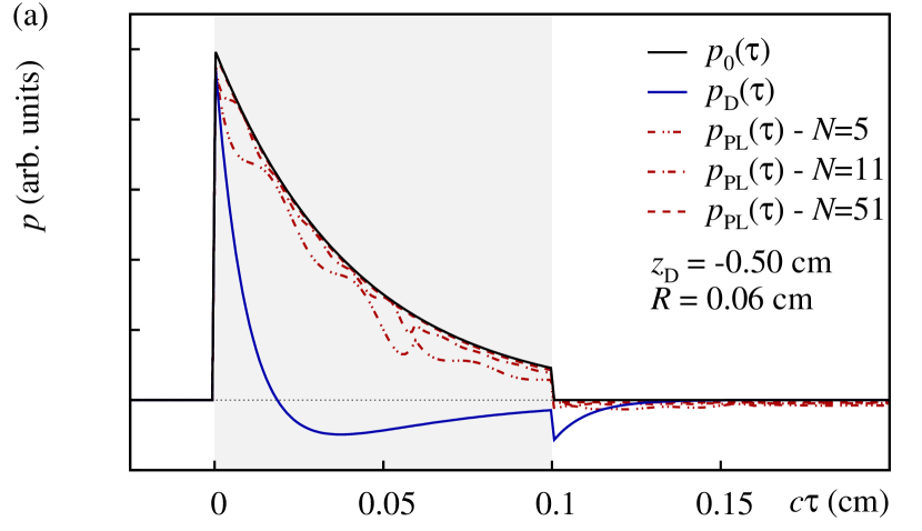
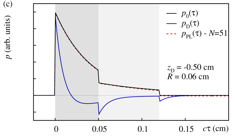
Figure 1: (Color online) Kernel and source reconstruction within the paraxial approximation for system parameters ${\bf p}_{\rm sys}=(c,a_{\rm B},z_{\rm D})\equiv(1\,{\rm cm/s},~{}0.1\,{\rm cm},~{}-0.5\,{\rm cm})$. (a) Inversion input $p_{\rm 0}$ (solid black line) and $p_{\rm D}$ (solid blue line) used to derive effective kernel for $N=5$, $11$, and $51$ Fourier-coefficients and cut-off parameter $R=0.06\,{\rm cm}$. Solution of the respective source reconstruction problems yields the estimates $p_{\rm PL}$ (dashed and dash-dotted red curves). (b) The main plot illustrates the effective kernel $\mathsf{K}_{\rm eff}(\Delta\tau)\equiv\mathsf{K}(\Delta\tau;{\bf a}^{\star},R)$ for two different cut-off distances $R=0.04\,{\rm cm}$, and $0.06\,{\rm cm}$. The inset shows the SSR $s(R)\equiv s({\bf a}^{\star},R)$ for $N=51$ as function of the cut-off distance where the minimum is attained at $R=0.06\,{\rm cm}$. (c) Solution $p_{\rm PL}$ of the source reconstruction problem for a OA signal $p_{\rm D}$ (solid blue line) resulting from a two-layer absorbing structure for the same system parameters as in (a). Source reconstruction is performed using the effective kernel for ${\bf p}_{\rm rec}=(51,0.06\,{\rm cm})$ resulting from the gauge procedure.

The inverse OA kernel reconstruction problem.

Note that the solution of the direct problem and inverse problem (I.1) in terms of Eq. (3) is feasible using standard numerical schemes based on, e.g., a trapezoidal approximation of the Volterra operator for a generic kernel Press et al. (1992), or highly efficient memoization techniques for the particular form of the above convolution kernel Stritzel et al. (2016). As pointed out earlier, considering inverse problem (I.2), we here suggest a Fourier-expansion of the Volterra kernel involving a sequence of $N$ expansion coefficients ${\bf a}\equiv\{a_{\ell}\}_{0\leq\ell<N}$ and a cut-off distance $R$ above which the resulting effective kernel is assumed to be zero, i.e.

$$\mathsf{K}(x;{\bf a},R)=\sum_{\ell=0}^{N-1}a_{\ell}\,k_{\ell}(x;R)\,\Theta(R-x).$$ (4)

The expansion functions $k_{\ell}(x;R)$ are given by

$$k_{\ell}(x;R)=\begin{cases}1,&\text{if }\ell=0\\ \cos\Big{(}2\pi\,\frac{\ell+1}{2}\frac{x}{R}\Big{)},&\text{if }\ell~{}\text{odd}\\ \sin\Big{(}2\pi\,\frac{\ell}{2}\frac{x}{R}\Big{)},&\text{if }\ell~{}\text{even}\end{cases}$$ (5)

and $\Theta(\cdot)$ signifies the Heavyside step-function. Then, for a suitable sequence ${\bf a}$, the Fourier approximation to the Volterra integral equation, Eq. (3), reads

$$p_{\rm D}(\tau)=p_{\rm 0}(\tau)-\sum_{\ell=0}^{N-1}a_{\ell}\,\mathsf{\Phi}_{\ell}(\tau;R),$$ (6)

with reduced partial diffraction terms

$$\mathsf{\Phi}_{\ell}(\tau;R)=\int_{-\infty}^{\tau}\!k_{\ell}(\tau-\tau^{\prime};R)\,\Theta(R-(\tau-\tau^{\prime}))\,p_{\rm 0}(\tau^{\prime})\,\mathrm{d}\tau^{\prime}.$$ (7)

Now, consider a given set of input data $(p_{\rm 0},p_{\rm D})$ for known apparative parameters ${\bf p}_{\rm sys}$, both in a discretized setting with constant mesh interval $\Delta$, mesh points $\{t_{i}\}_{0\leq i\leq M}$ where $t_{0}=0$, $t_{i}=t_{i-1}+\Delta$, and $t_{M}$ large enough to ensure a reasonable measurement depth. Then, bearing in mind that $\tau_{i}=t_{i}+z_{\rm D}/c$, the optimal expansion coefficient sequence ${\bf a}^{\star}$ can be obtained by minimizing the sum of the squared residuals (SSR)

$$s({\bf a},R)=\sum_{i=0}^{M}\Big{[}(p_{\rm 0}(\tau_{i})-p_{\rm D}(\tau_{i}))\,-\,\sum_{\ell=0}^{N-1}a_{\ell}\,\mathsf{\Phi}_{\ell}(\tau_{i};R)\Big{]}^{2}.$$ (8)

In the above optimization formulation of inverse problem (I.2), we considered a trapezoidal rule to numerically evaluate the integrals that enter via the functions $\mathsf{\Phi}_{\ell}(\tau_{i};R)$. In an attempt to construct an effective Volterra kernel $\mathsf{K}(x;{\bf a},R)$ for a controlled setup with a priori known parameters ${\bf p}_{\rm sys}$, one might use the high-precision “Gaussian-beam” estimator $a_{\ell}=(2\omega_{\rm D}/R)\int_{0}^{R}\!k_{\ell}(x;R)\,\exp\{-\omega_{\rm D}x\}\,\mathrm{d}x$ to obtain an initial sequence ${\bf a}_{\rm 0}$ of expansion coefficients by means of which a least-squares routine for the minimization of Eq. (8) might be started. In a situation where, say, $a_{\rm B}$ is only known approximately or the assumption of a Gaussian beam profile is violated, one has to rely on a rather low-precision coefficient estimate obtained by roughly estimating the apparative parameters and resorting on the above “Gaussian-beam” estimate.

An exemplary kernel reconstruction procedure is shown in FIG. 1, where the OA signal $p_{\rm D}$ at ${\bf p}_{\rm sys}=(1\,{\rm cm/s},~{}0.1\,{\rm cm},~{}-0.5\,{\rm cm})$, i.e. $D\approx 3.75$, is first obtained by solving the direct OA problem for Eq. (3) for an absorbing layer with $\mu_{a}=24\,{\rm cm^{-1}}$ in the range $z=0-0.1\,{\rm cm}$, see black ($p_{\rm 0}$) and blue ($p_{\rm D}$) curves in FIG. 1(a). The set $(p_{\rm 0},p_{\rm D})$ is then used as inversion input to compute the effective Volterra kernel for various sets of reconstruction parameters ${\bf p}_{\rm rec}=(N,R)$. In particular, considering $N=51$, the minimal value of $s({\bf a}^{\star},R^{\star})\approx 1.47$ is attained at $R^{\star}=0.06\,{\rm cm}$, see the inset of FIG. 1(b). As evident from the main plot of FIG. 1(b), the effective Volterra kernel for ${\bf p}_{\rm rec}=(51,R^{\star})$ follows the exact stress wave propagator for almost two orders of magnitude up to $c\Delta\tau\approx 0.05\,{\rm cm}$. Beyond that limit, the noticeable deviation between both does not seem to affect the overall SSR $s({\bf a},R)$ too much. In this regard, note that the kernel approximated for the (non optimal) choice ${\bf p}_{\rm rec}=(51,0.04\,{\rm cm})$ exhibits a worse SSR.

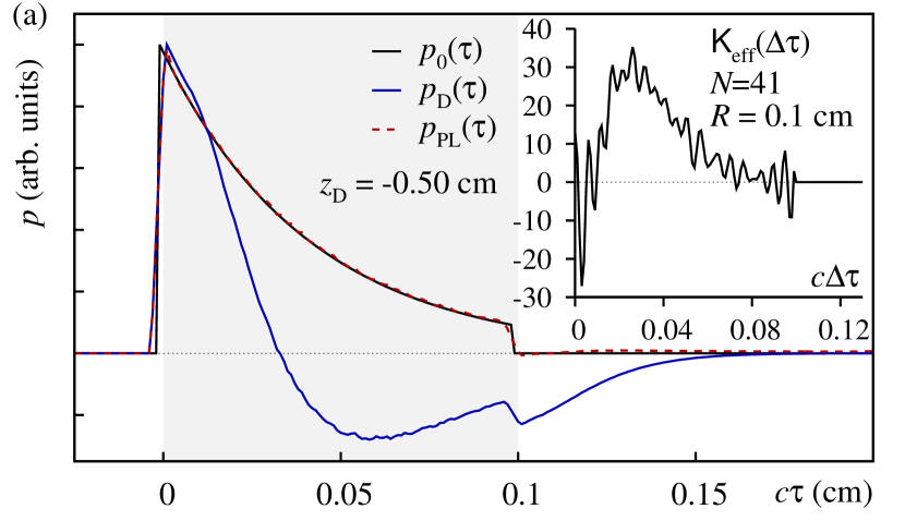
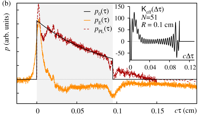
Figure 2: (Color online) Inversion of OA signals to initial stress profiles beyond the paraxial approximation. Both figures illustrate the kernel and source reconstruction procedures for (a) inversion of an OA signal featuring a top-hat irradiation source profile (see text). The main plot shows the input $(p_{\rm 0},p_{\rm D})$ to the inversion procedure (solid black and blue lines, respectively) as well as the reconstructed initial stress profile $p_{\rm PL}$ (dashed red line), and, (b) inversion of an OA signal resulting from an actual measurement Blumenröther et al. (2016). The main plot shows the synthetic initial stress profile $p_{\rm 0}$ (solid black line) used during the gauge procedure as well as the inversion input $p_{\rm E}$ (orange line) for which the reconstructed initial stress profile $p_{\rm PL}$ (dashed red line) is obtained. In both figures, the inset illustrates the effective Volterra kernel resulting from the Fourier-approximation.

The inverse OA source reconstruction problem.

Note that the above Fourier-expansion approximation might be interpreted as a gauge procedure to adjust an effective Volterra kernel $\mathsf{K}(x;{\bf a}^{\star},R)$ for an (possibly unknown) apparative setup ${\bf p}_{\rm sys}$, here indirectly accessible through the diffraction transformation of the OA signal $p_{\rm D}$ relative to $p_{\rm 0}$. That is, once the kernel reconstruction (I.2) is accomplished for a set of reference curves $(p_{\rm 0},p_{\rm D})_{\rm ref}$ under ${\bf p}_{\rm sys}$, the source reconstruction problem (I.1) might subsequently be tackled also for all other OA signals measured under ${\bf p}_{\rm sys}$ by solving the OA Volterra integral equation Eq. (3) in terms of a Picard-Lindelöf “correction” scheme Hairer et al. (1993). The latter is based on the continued refinement of a putative solution, starting off from a properly guessed “predictor” $p_{\rm PL}^{(0)}(\tau)$, improved successively by solving

$$p_{\rm PL}^{(n+1)}(\tau)=p_{\rm D}(\tau)+\int_{-\infty}^{\tau}\!\mathsf{K}(\tau-\tau^{\prime};{\bf a}^{\star},R)\,p_{\rm PL}^{(n)}(\tau^{\prime})\,\mathrm{d}\tau^{\prime}.$$ (9)

From a practical point of view we terminated the iterative correction scheme as soon as the ${\rm max}$-norm $c_{n}\equiv\|p_{\rm PL}^{(n+1)}(\tau)-p_{\rm PL}^{(n)}(\tau)\|$ of two successive solutions decreases below $c_{n}\leq 10^{-6}$. We here refer to the final estimate simply as $p_{\rm PL}$. Note that, attempting a solution of (I.1) in the acoustic near-field, a high-precision predictor can be obtained by using the initial guess $p_{\rm PL}^{(0)}\equiv p_{\rm D}$. This is a reasonable choice since one might expect the change of the OA near-field signal due to diffraction to be still quite small. Further, source reconstruction in the acoustic far-field might be started using a high-precision predictor obtained by integrating the OA signal $p_{\rm D}$ in the far-field approximation Stritzel et al. (2016). In contrast to this, low-precision predictors for both cases can be obtained by setting $p_{\rm PL}^{(0)}\equiv c_{\rm 0}$, where, e.g., $c_{\rm 0}=0$.

The solution of the source reconstruction problem for the OA signal $p_{\rm D}$ used in the approximation of the Volterra kernel for the above setting ${\bf p}_{\rm sys}=(1\,{\rm cm/s},\,0.1\,{\rm cm},\,-0.5\,{\rm cm})$ is shown in FIG. 1(a). The apparent agreement of the data curves $p_{\rm PL}$ for ${\bf p}_{\rm rec}=(51,R^{\star})$ and $p_{\rm 0}$ does not come as a surprise since $p_{\rm D}$ was used for the gauge procedure in the first place. As a remedy we attempt a source reconstruction for a second independent OA signal, simulated for the same apparative setting only with two absorbing layers $\mu_{a,1}=24\,{\rm cm^{-1}}$ from $z=0-0.05\,{\rm cm}$ and $\mu_{a,2}=12\,{\rm cm^{-1}}$ from $z=0.05-0.12\,{\rm cm}$. As evident from FIG. 1(c), inversion using the effective Volterra kernel from the previous gauge procedure yields a reconstructed stress profile $p_{\rm PL}$ in excellent agreement with the underlying exact initial stress profile $p_{\rm 0}$.

Inversion beyond the paraxial approximation.

Given the apparent feasibility of the kernel reconstruction routine as a gauge procedure to model the diffraction transformation of OA signals in terms of an effective stress wave propagator in the framework of the OA Volterra integral equation, we next address the inversion of OA signals to initial stress profiles beyond the paraxial approximation. Therefore, we first consider a borderline far-field signal for a top-hat irradiation source

$$f(\vec{r}_{\perp})=\begin{cases}1,&\text{if }|\vec{r}_{\perp}|\leq\rho_{0}\\ \exp\{-(|\vec{r}_{\perp}|-\rho_{0})^{2}/a_{\rm B}^{2}\},&\text{if }|\vec{r}_{\perp}|>\rho_{0}\end{cases},$$ (10)

recorded at the system parameters ${\bf p}_{\rm sys}=(c,\rho_{0},a_{\rm B},z_{\rm D})=(1\,{\rm cm/s},\,0.1\,{\rm cm},\,0.1\,{\rm cm},\,-0.50\,{\rm cm})$, and thus $D=2|z_{\rm D}|/(\mu_{\rm a}(a_{\rm B}+\rho_{0}))\approx 1.04$, obtained via an independent forward solver for the full OA wave equation designed for the solution of the OA Poisson integral for layered media Wang (2009); Blumenröther et al. (2016). The inversion results are summarized in FIG. 2(a), where the kernel reconstruction (inset) and source reconstruction (main plot) are shown for the parameter set ${\bf p}_{\rm rec}=(41,\,0.1\,{\rm cm})$. The excellent agreement of the stress profiles $p_{\rm 0}$ and $p_{\rm PL}$ suggests that the kernel reconstruction routine also applies to a more general OA setting, based on the full OA wave equation. Finally, we consider an OA signal resulting from an actual measurement on PVA hydrogel based tissue phantoms Blumenröther et al. (2016). In this case we carefully estimated the apparative parameters ${\bf p}_{\rm sys}=(150000\,{\rm cm/s},\,0.054\,{\rm cm},0.081{\rm cm/s},\,-0.3\,{\rm cm})$ as well as $\mu_{a}=11\,{\rm cm}$ in the range $z=0-0.095\,{\rm cm}$, i.e. $D\approx 6.73$, in order to create a set of synthetic input data by means of which an appropriate kernel gauge procedure can be carried out. The result of the procedure using ${\bf p}_{\rm rec}=(51,\,0.1\,{\rm cm})$ is shown in FIG. 2(b). So as to perform the source reconstruction for the experimental signal $p_{\rm E}$, we considered data within the interval $c\tau=[0,\,0.15]\,{\rm cm}$, only. As evident from the figure, the reconstructed stress profile $p_{\rm PL}$ fits the signal $p_{\rm 0}$ used in the gauge procedure remarkably well .

Conclusions.

In the presented Letter we have introduced and discussed the kernel reconstruction problem in the paraxial approximation to the optoacoustic wave equation. We suggested a Fourier-expansion approach to approximate the Volterra kernel which takes a central role in the theoretical framework. The developed approach proved useful as gauge procedure by means of which the diffraction transformation experienced by OA signals can effectively be modeled, allowing to subsequently solve the source reconstruction problem in the underlying apparative setting. From this numerical study we found that the developed approach extends beyond the framework of the paraxial approximation and also allows for the inversion of OA signals described by the full OA wave equation. From a point of view of computational theoretical physics it would be tempting to explore other kernel expansions in terms of generalized Fourier series as well as gauge procedures involving sets of measured pressure profiles only. Such investigations are currently in progress with the aim to shed some more light on this intriguing inverse problem in the field of optoacoustics and to facilitate a complementary approach to conventional OA imaging.

References

- Diebold et al. (1990) G. J. Diebold, M. I. Khan, and S. M. Park, Science 250, 101 (1990).
- Diebold et al. (1991) G. J. Diebold, T. Sun, and M. I. Khan, Phys. Rev. Lett. 67, 3384 (1991).
- Calasso et al. (2001) I. G. Calasso, W. Craig, and G. J. Diebold, Phys. Rev. Lett. 86, 3550 (2001).
- Gusev and Karabutov (1993) V. E. Gusev and A. A. Karabutov, Laser Optoacoustics (American Institute of Physics, 1993).
- Landau and Lifshitz (1981) L. D. Landau and E. M. Lifshitz, Hydrodynamik (4th Ed.) (Akademie-Verlag (Berlin), 1981).
- Colton and Kress (2013) D. Colton and R. Kress, Inverse Acoustic and Electromagnetic Scattering Theory (3rd Ed.) (Springer, 2013).
- Wang (2009) L. Wang, Photoacoustic Imaging and Spectroscopy, Optical Science and Engineering (CRC Press, 2009).
- Kuchment and Kunyansky (2008) P. Kuchment and L. Kunyansky, European Journal of Applied Mathematics 19, 191 (2008).
- Xu and Wang (2006) M. Xu and L. V. Wang, Rev. Sci. Instr. 77, 041101 (2006).
- Wang and Hu (2012) L. V. Wang and S. Hu, Science 335, 1458 (2012).
- Yang et al. (2012) J.-M. Yang, C. Favazza, R. Chen, J. Yao, X. Cai, K. Maslov, Q. Zhou, K. K. Shung, and L. V. Wang, Nature medicine 18, 1297 (2012).
- Wang et al. (2013) L. Wang, J. Xia, J. Yao, K. I. Maslov, and L. V. Wang, Phys. Rev. Lett. 111, 204301 (2013).
- Wang et al. (2014) L. Wang, C. Zhang, and L. V. Wang, Phys. Rev. Lett. 113, 174301 (2014).
- Stoffels et al. (2015a) I. Stoffels, S. Morscher, I. Helfrich, U. Hillen, J. Leyh, N. C. Burton, T. C. P. Sardella, J. Claussen, T. D. Poeppel, H. S. Bachmann, A. Roesch, K. Griewank, D. Schadendorf, M. Gunzer, and J. Klode, Science Translational Medicine 7, 317ra199 (2015a).
- Stoffels et al. (2015b) I. Stoffels, S. Morscher, I. Helfrich, U. Hillen, J. Leyh, N. C. Burton, T. C. P. Sardella, J. Claussen, T. D. Poeppel, H. S. Bachmann, A. Roesch, K. Griewank, D. Schadendorf, M. Gunzer, and J. Klode, Science Translational Medicine 7, 319er8 (2015b).
- Agranovsky and Kuchment (2007) M. Agranovsky and P. Kuchment, Inverse Problems 23, 2089 (2007).
- Deán-Ben et al. (2012) X. L. Deán-Ben, A. Buehler, V. Ntziachristos, and D. Razansky, IEEE Transactions on Medical Imaging 31, 1922 (2012).
- Belhachmi et al. (2016) Z. Belhachmi, T. Glatz, and O. Scherzer, Inverse Problems 32, 045005 (2016).
- Norton and Linzer (1981) S. J. Norton and M. Linzer, IEEE Trans. Biomed. Eng. , 202 (1981).
- Xu and Wang (2005) M. Xu and L. V. Wang, Phys. Rev. E 71, 016706 (2005).
- Burgholzer et al. (2007) P. Burgholzer, G. J. Matt, M. Haltmeier, and G. Paltauf, Phys. Rev. E 75, 046706 (2007).
- Chadan and Sabatier (1989) K. Chadan and P. Sabatier, Inverse Problems of Quantum Scattering Theory (Springer, 1989).
- Apagyi et al. (1997) B. Apagyi, G. Endrédi, and P. Levay, Inverse and Algebraic Quantum Scattering Theory, Lecture notes in physics (Springer, 1997).
- Münchow and Scheid (1980) M. Münchow and W. Scheid, Phys. Rev. Lett. 44, 1299 (1980).
- Melchert et al. (2006) O. Melchert, W. Scheid, and B. Apagyi, J. Phys. G: Nucl. Part. Phys. 32, 849 (2006).
- Tam (1986) A. C. Tam, Rev. Mod. Phys. 58, 381 (1986).
- Karabutov et al. (1996) A. Karabutov, N. B. Podymova, and V. S. Letokhov, Appl. Phys. B 63, 545 (1996).
- Press et al. (1992) W. Press, B. Flannery, S. Teukolsky, and W. Vetterling, Numerical Recipes in FORTRAN 77 (Cambridge University Press, 1992).
- Stritzel et al. (2016) J. Stritzel, O. Melchert, M. Wollweber, and B. Roth, “Direct and inverse solver for the 3D optoacoustic Volterra equation,” (2016), (unpublished), arXiv:1606.04740 .
- Blumenröther et al. (2016) E. Blumenröther, O. Melchert, M. Wollweber, and B. Roth, “Detection, numerical simulation and approximate inversion of optoacoustic signals generated in multi-layered PVA hydrogel based tissue phantoms,” (2016), (unpublished), arXiv:1605.05657 .
- Hairer et al. (1993) E. Hairer, S. P. Nørsett, and G. Wanner, Solving Ordinary Differential Equations I (2nd rev. Ed.): Nonstiff Problems (Springer, 1993).
- Note (1) A Python implementation of our code for the solution of inverse problems (I.1) and (I.2) can be found at https://github.com/omelchert/INVERT.git.