Rosseland and flux mean opacities for Compton scattering

Abstract

Rosseland mean opacity plays an important role in theories of stellar evolution and X-ray burst models. In the high-temperature regime, when most of the gas is completely ionized, the opacity is dominated by Compton scattering. Our aim here is to critically evaluate previous works on this subject and to compute exact Rosseland mean opacity for Compton scattering in a broad range of temperatures and electron degeneracy parameter. We use relativistic kinetic equations for Compton scattering and compute the photon mean free path as a function of photon energy by solving the corresponding integral equation in the diffusion limit. As a byproduct we also demonstrate the way to compute photon redistribution functions in case of degenerate electrons. We then compute the Rosseland mean opacity as a function of temperature and electron degeneracy. We compare our results to the previous calculations and find a significant difference in the low-temperature regime and strong degeneracy. We find useful analytical expressions that approximate well the numerical results. We then proceed to compute the flux mean opacity and show that in diffusion approximation it is nearly identical to the Rosseland mean opacity. We also provide a simple way for accounting for the true absorption in evaluation of the Rosseland and flux mean opacities.

Submitted to The Astrophysical Journal

1 Introduction

The key role in the description of the radiation transport through the medium is played by two average opacities. The first one, known as the Rosseland mean opacity

$$\kappa_{\rm R}=\int_{0}^{\infty}d\nu\ \left(\partial B_{\nu}/\partial T\right)\left/\int_{0}^{\infty}d\nu\ \kappa_{\nu}^{-1}\left(\partial B_{\nu}/\partial T\right),\right.$$ (1)

relates the temperature gradient to the radiation flux:

$$\mbox{\boldmath$F$}=-\frac{ac}{3\kappa_{\rm R}}\mbox{\boldmath$\nabla$}{T^{4}}.$$ (2)

The second one, known as the flux mean opacity

$$\kappa_{\rm F}=\left.\int_{0}^{\infty}d\nu\ \kappa_{\nu}\ F_{\nu}\right/F,$$ (3)

relates the bolometric radiation flux to the radiative acceleration (see Mihalas & Mihalas, 1984, pp. 360-361):

$$\mbox{\boldmath$g$}_{\rm rad}=\frac{\kappa_{\rm F}}{c}\mbox{\boldmath$F$}.$$ (4)

The Rosseland mean can be easily computed once the total, absorption and scattering, opacity as a function of photon frequency $\kappa_{\nu}$ is known. For the flux mean, we also need to specify the spectral energy distribution given by the flux $F_{\nu}$. However, in the diffusion approximation these two opacities coincide for pure absorption and coherent scattering.

In the high-temperature regime, when most of the gas is completely ionized, the opacity is dominated by Compton scattering. This situation is not so simple as the scattering is incoherent, induced scattering has to be accounted for and instead of the total cross-section the effective cross-section should be used. The case of the non-degenerate electron gas was considered by Sampson (1959). It was further extended by Chin (1965) to include the effect of electron degeneracy. This work was affected by an error, which also propagated to the textbooks (Chiu, 1968; Cox & Giuli, 1968; Weiss et al., 2004). The corrected method to compute the Rosseland mean was introduced by Buchler & Yueh (1976), who provide also a comprehensive analysis of the previous results. The numerical results presented in that work were approximated by Paczynski (1983) with a simple analytical expression, which were later used in numerous papers on X-ray bursts. An alternative approximation was given by Weaver et al. (1978).

In this paper we recompute the Rosseland and the flux mean opacities for Compton scattering and compare our results to the previous calculations. We also provide new analytical formulae that approximate well the numerical results.

2 Relativistic kinetic equation for Compton scattering

Derivation of the Rosseland mean opacity for Compton scattering is based on solution of the relativistic kinetic equation (RKE) in terms of the photon mean-free path as a function of its energy. Interaction between photons and electrons (positrons) via Compton scattering accounting for the induced scattering and fermion degeneracy can be described by the explicitly covariant RKE for photons (Buchler & Yueh, 1976; de Groot et al., 1980; Nagirner & Poutanen, 1993, 1994):

$$\underline{x}\cdot\underline{\nabla}n(\mbox{\boldmath$x$}) = \frac{r_{\rm e}^{2}}{2}\frac{2}{\lambda_{\rm C}^{3}}\int\frac{{d}\mbox{\boldmath$p$}}{\gamma}\frac{{d}\mbox{\boldmath$p$}_{1}}{\gamma_{1}}\frac{{d}\mbox{\boldmath$x$}_{1}}{x_{1}}\>F\>\delta^{4}(\underline{p}_{1}+\underline{x}_{1}-\underline{p}-\underline{x})$$

$$\times \left\{n(\mbox{\boldmath$x$}_{1})[1+n(\mbox{\boldmath$x$})]\left[\tilde{n}_{-}(\mbox{\boldmath$p$}_{1})(1\!-\!\tilde{n}_{-}(\mbox{\boldmath$p$}))+\tilde{n}_{+}(\mbox{\boldmath$p$}_{1})(1\!-\!\tilde{n}_{+}(\mbox{\boldmath$p$}))\right]\right.$$

$$- \left.n(\mbox{\boldmath$x$})[1+n(\mbox{\boldmath$x$}_{1})]\left[\tilde{n}_{-}(\mbox{\boldmath$p$})(1\!-\!\tilde{n}_{-}(\mbox{\boldmath$p$}_{1}))+\tilde{n}_{+}(\mbox{\boldmath$p$})(1\!-\!\tilde{n}_{+}(\mbox{\boldmath$p$}_{1}))\right]\right\},$$

where $\underline{\nabla}=\{\partial/c\partial t,-\mbox{\boldmath$\nabla$}\}$ is the four-gradient, $r_{\rm e}$ is the classical electron radius, $\lambda_{\rm C}=h/m_{\rm e}c$ is the Compton wavelength. Here we defined the dimensionless photon four-momentum as $\underline{x}=\{x,\mbox{\boldmath$x$}\}=x\{1,\mbox{\boldmath$\hat{\omega}$}\}$, where $\hat{\omega}$ is the unit vector in the photon propagation direction and $x\equiv h\nu/m_{\rm e}c^{2}$ is the photon energy in units of the electron rest mass. The photon distribution is described by the occupation number $n$. The dimensionless electron/positron four-momentum is $\underline{p}=\{\gamma,\mbox{\boldmath$p$}\}=\{\gamma,p\mbox{\boldmath$\hat{\Omega}$}\}=\gamma\{1,\beta\mbox{\boldmath$\hat{\Omega}$}\}$, where $\hat{\Omega}$ is the unit vector along the electron momentum, $\gamma$ and $p=\sqrt{\gamma^{2}-1}$ are the electron Lorentz factor and its momentum in units of $m_{\rm e}c$ and $\beta$ is the velocity in units of $c$. The electron/positron distributions are described by the occupation numbers $\tilde{n}_{\pm}$.

The factor $F$ in Equation (2) is the Klein–Nishina reaction rate (Berestetskii et al., 1982)

$$F=\left(\frac{1}{\xi}-\frac{1}{\xi_{1}}\right)^{2}+2\;\left(\frac{1}{\xi}-\frac{1}{\xi_{1}}\right)+\frac{\xi}{\xi_{1}}+\frac{\xi_{1}}{\xi},$$ (6)

and

$$\xi=\underline{p}_{1}\cdot\underline{x}_{1}=\underline{p}\cdot\underline{x},\qquad\xi_{1}=\underline{p}_{1}\cdot\underline{x}=\underline{p}\cdot\underline{x}_{1}$$ (7)

are the four-products of the corresponding momenta. Second equalities in Eqs. (7) arise from the four-momentum conservation law represented by the delta-function in Eq. (2).

The electron/positron distribution under assumption of thermal equilibrium and isotropy, is given by the Fermi-Dirac distribution:

$$\tilde{n}_{\pm}(\mbox{\boldmath$p$})=\frac{1}{\displaystyle\exp\left(\frac{\gamma-1}{\Theta}-\eta_{\pm}\right)+1},$$ (8)

where $\Theta=kT/m_{\rm e}c^{2}$ is the dimensionless temperature and $\eta_{\pm}$ are the degeneracy parameters for positron and electrons (the ratio of the Fermi energy minus rest mass to temperature) related via $\eta_{-}+\eta_{+}=-2/\Theta$ (see e.g. Cox & Giuli 1968; page 302 of Weiss et al. 2004). The electron/positron concentrations are given by the integrals over the momentum space:

$$N_{\pm}=4\pi\frac{2}{\lambda_{\rm C}^{3}}\int_{0}^{\infty}p^{2}{d}p\ \tilde{n}_{\pm}(\mbox{\boldmath$p$}),$$ (9)

and the density (not including electrons and positrons created by pair-production as well as radiation) is

$$\rho=(N_{-}-N_{+})\mu_{\rm e}m_{\rm p},$$ (10)

where $\mu_{\rm e}=2/(1+X)$ is the mean number of nucleons per free ionization electron and $X$ is the hydrogen mass fraction. The total number density of electrons and positrons is $N_{\rm e}=N_{-}+N_{+}$.

The form of the RKE (2) can be simplified by defining the redistribution functions (RF) via

$$R_{\pm}(\mbox{\boldmath$x$}_{1}\rightarrow\mbox{\boldmath$x$})=\frac{3}{16\pi}\frac{2}{\lambda_{\rm C}^{3}}\frac{1}{N_{\pm}}\int\!\frac{{d}\mbox{\boldmath$p$}}{\gamma}\frac{{d}\mbox{\boldmath$p$}_{1}}{\gamma_{1}}\tilde{n}_{\pm}(\mbox{\boldmath$p$}_{1})[1-\tilde{n}_{\pm}(\mbox{\boldmath$p$})]\ F\ \delta^{4}(\underline{p}_{1}+\underline{x}_{1}-\underline{p}-\underline{x}).$$ (11)

The RFs satisfy the symmetry property

$$R_{\pm}(\mbox{\boldmath$x$}\rightarrow\mbox{\boldmath$x$}_{1})\ e^{-x/\Theta}=R_{\pm}(\mbox{\boldmath$x$}_{1}\rightarrow\mbox{\boldmath$x$})\ e^{-x_{1}/\Theta},$$ (12)

which follows from its definition (11) and the energy conservation $\gamma_{1}=\gamma+x-x_{1}$, or from the detailed balance condition (see eq. 8.2 in Pomraning 1973).

In the absence of strong magnetic field, the medium is isotropic, therefore the RF depends only on the photon energies and the scattering angle (with $\mu$ being its cosine), i.e. we can write $R_{\pm}(\mbox{\boldmath$x$}_{1}\rightarrow\mbox{\boldmath$x$})=R_{\pm}(x,x_{1},\mu)$. Introducing the total RF as

$$R(x,x_{1},\mu)=\frac{N_{-}}{N_{\rm e}}R_{-}(x,x_{1},\mu)+\frac{N_{+}}{N_{\rm e}}R_{+}(x,x_{1},\mu),$$ (13)

the kinetic equation (2) in a steady-state can be recast in a standard form of the radiative transfer equation

$$\mbox{\boldmath$\hat{\omega}$}\cdot\mbox{\boldmath$\nabla_{\tau}$}n(\mbox{\boldmath$x$})=-n(\mbox{\boldmath$x$})\frac{1}{x}\int_{0}^{\infty}\!\!\!\!x_{1}{d}x_{1}\!\!\int\!\!{d}^{2}\mbox{\boldmath$\hat{\omega}$}_{1}\>R(x_{1},x,\mu)\ [1+n(\mbox{\boldmath$x$}_{1})]+[1+n(\mbox{\boldmath$x$})]\frac{1}{x}\int_{0}^{\infty}\!\!\!\!x_{1}{d}x_{1}\!\!\int\!\!{d}^{2}\mbox{\boldmath$\hat{\omega}$}_{1}\>R(x,x_{1},\mu)\ n(\mbox{\boldmath$x$}_{1}),$$ (14)

where $\mbox{\boldmath$\nabla_{\tau}$}=\mbox{\boldmath$\nabla$}/\sigma_{\rm T}N_{\rm e}$ is the dimensionless gradient, with $\sigma_{\rm T}$ being the Thomson cross-section.

3 Photon mean free path

Deep inside stars or thermonuclear burning regions of X-ray bursts, radiation field is nearly isotropic and the diffusion approximation should be rather accurate. We therefore can express the occupation number as

$$n(\mbox{\boldmath$x$})=b_{x}-{l_{x}}\mbox{\boldmath$\hat{\omega}$}\cdot\mbox{\boldmath$\nabla_{\tau}$}b_{x},$$ (15)

where $b_{x}=1/[\exp(x/\Theta)-1]$ is the occupation number for the Planck distribution and $l_{x}$ is the mean free path (in units of $1/\sigma_{\rm T}N_{\rm e}$) for Compton scattering of a photon of energy $x$. Substituting expansion (15) to Eq. (14), noticing that the zeroth order terms cancel out, keeping only terms of the first order in $\mbox{\boldmath$\nabla_{\tau}$}b_{x}$, and using condition (12), we get (Sampson, 1959; Buchler & Yueh, 1976):

$$\mbox{\boldmath$\hat{\omega}$}\cdot\mbox{\boldmath$\nabla_{\tau}$}b_{x}\!=\!\frac{1}{x}\int_{0}^{\infty}\!\!\!\!x_{1}{d}x_{1}\!\!\int\!{d}^{2}\mbox{\boldmath$\hat{\omega}$}_{1}\>R(x_{1},x,\mu)\left[l_{x}\mbox{\boldmath$\hat{\omega}$}\cdot\mbox{\boldmath$\nabla_{\tau}$}b_{x}\left(\frac{1-e^{-x/\Theta}}{1-e^{-x_{1}/\Theta}}\right)-l_{x_{1}}\mbox{\boldmath$\hat{\omega}$}_{1}\cdot\mbox{\boldmath$\nabla_{\tau}$}b_{x_{1}}\left(\frac{e^{x_{1}/\Theta}-1}{e^{x/\Theta}-1}\right)\right].$$ (16)

Simple algebra gives a linear integral equation for the mean free path $l_{x}$:

$$1=\frac{1}{x}\int_{0}^{\infty}\!\!\!\!x_{1}{d}x_{1}\!\!\int\!{d}^{2}\mbox{\boldmath$\hat{\omega}$}_{1}\>R(x_{1},x,\mu)\frac{1-e^{-x/\Theta}}{1-e^{-x_{1}/\Theta}}\left[l_{x}-l_{x_{1}}\frac{x_{1}}{x}\frac{\mbox{\boldmath$\hat{\omega}$}_{1}\cdot\mbox{\boldmath$\nabla$}\Theta}{\mbox{\boldmath$\hat{\omega}$}\cdot\mbox{\boldmath$\nabla$}\Theta}\right].$$

Choosing the coordinate system so that $\mbox{\boldmath$\hat{\omega}$}=(0,0,1)$, defining $\mbox{\boldmath$\hat{\omega}$}_{1}=\left(\sqrt{1-\mu^{2}}\cos\phi,\sqrt{1-\mu^{2}}\sin\phi,\mu\right)$ and $\nabla\Theta\propto(\sin\theta,0,\cos\theta)$, the integral over solid angle becomes $\int{d}\mu\int{d}\phi$, with only the last term in the square brackets depending on $\phi$. The azimuthal integral is then

$$\int_{0}^{2\pi}\!\!\!\!\!{d}\phi\frac{\mbox{\boldmath$\hat{\omega}$}_{1}\cdot\mbox{\boldmath$\nabla$}\Theta}{\mbox{\boldmath$\hat{\omega}$}\cdot\mbox{\boldmath$\nabla$}\Theta}=\!\!\int_{0}^{2\pi}\!\!\!\!{d}\phi\ \left(\mu+\sqrt{1-\mu^{2}}\tan\theta\cos\phi\right)=2\pi\mu,$$ (17)

so that the square bracket in Eq. (3) can be substituted by $l_{x}-l_{x_{1}}x_{1}\mu/x$ (Sampson, 1959). Equation (3) can be further modified by integrating over the angles of the scattered photon:

$$1=4\pi\int\limits_{0}^{\infty}\frac{x_{1}}{x}{d}x_{1}\frac{1-e^{-x/\Theta}}{1-e^{-{x_{1}}/{\Theta}}}\left[l_{x}R_{0}(x_{1},x)-l_{x_{1}}\!\frac{x_{1}}{x}R_{1}(x_{1},x)\right],$$ (18)

where we introduced the moments of the RF (Nagirner & Poutanen, 1994)

$$R_{0}(x_{1},x) = \frac{1}{2}\int_{-1}^{1}R(x_{1},x,\mu){d}\mu,$$ (19)

$$R_{1}(x_{1},x) = \frac{1}{2}\int_{-1}^{1}R(x_{1},x,\mu)\ \mu\ {d}\mu.$$ (20)

The method for computing these functions is described in Appendix A.

At low temperatures the RFs are extremely peaked at $x_{1}\approx x$ and therefore two approximations are often made (Sampson, 1959; Buchler & Yueh, 1976):

$$l_{x_{1}} \approx l_{x},$$ (21)

$$\frac{1-e^{-x/\Theta}}{1-e^{-{x_{1}}/{\Theta}}} \approx 1.$$ (22)

The first approximation is equivalent to the on-the-spot approximation in the theory of radiative transfer in spectral lines. These approximations reduce Eq. (18) for the mean free path to

$$\frac{1}{l_{x}}\approx s_{0}(x)-s_{1}(x),$$ (23)

where (Nagirner & Poutanen, 1994)

$$s_{i}(x)=\frac{4\pi}{x^{i+1}}\int x_{1}^{i+1}{d}x_{1}R_{i}(x_{1},x),\quad i=0,1.$$ (24)

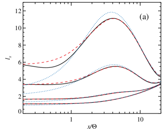
Figure 1: Mean-free path of photons $l_{x}$ as a function of photon energy to temperature ratio for various temperatures and degeneracies: (a) for $\Theta=0.05$, (b) $\Theta=0.25$, (c) $\Theta=0.5$. Different lines from bottom to the top correspond to the degeneracy parameter $\eta=-2,1,4,7$. The exact solution (18) are shown by the solid black lines. The approximate expressions (23) and (25) are shown by the dotted blue and dashed red lines, respectively.

At temperatures above 50 keV, approximation (22) fails (see Fig. 1). Still keeping the on-the-spot approximation (21), we get an explicit expression

$$\frac{1}{l_{x}}\approx r_{0}(x)-r_{1}(x),$$ (25)

where

$$r_{i}(x)=\frac{4\pi}{x^{i+1}}\int x_{1}^{i+1}{d}x_{1}R_{i}(x_{1},x)\frac{1-e^{-x/\Theta}}{1-e^{-{x_{1}}/{\Theta}}}.$$ (26)

At low temperatures, the easiest way to exactly solve Eq. (18) for $l_{x}$ is to use iteration procedure, starting from the approximation (25). The functions $r_{i}(x)$ can be tabulated in advance. The integrals over the energy $x_{1}$ for every $x$ have to be taken over a dense grid around $x$. For high temperatures, in principle, one can replace the integral by the discrete sum on a logarithmic grid of photon energies $x_{i}$ and solve Eq. (18) as a system of linear equations for $l_{i}=l_{x_{i}}$ (as was done by Buchler & Yueh 1976):

$$\frac{1}{4\pi}=l_{i}\ a_{i}+\sum_{j}\ l_{j}\ b_{ij}=\sum_{j}\ l_{j}\ (b_{ij}+a_{i}\delta_{ij}),$$ (27)

where

$$a_{i} = \sum_{j}\!w_{j}\frac{x_{j}}{x_{i}}\frac{1-e^{-x_{i}/\Theta}}{1-e^{-{x_{j}}/{\Theta}}}R_{0}(x_{j},x_{i}),$$ (28)

$$b_{ij} = -w_{j}\frac{x_{j}^{2}}{x_{i}^{2}}\frac{1-e^{-x_{i}/\Theta}}{1-e^{-{x_{j}}/{\Theta}}}R_{1}(x_{j},x_{i}),$$ (29)

and $w_{j}$ are the integration weights (equal to $x_{j}\ \Delta\ln x$ for a log-grid), $\delta_{ij}$ is the Kronecker delta. The results of calculations for $l_{x}$ using solution of the integral equation as well as by approximate formulae (25) and (23) are presented in Fig. 1.

We see that the mean free path computed using expression (25) approximates well the exact $l_{x}$ at all photon energies $x$ for low temperatures and small degeneracy parameter $\eta$ as well as at $x\gtrsim\Theta$ for large $\Theta$ and $\eta$. The approximate expression (23) used by Sampson (1959) is also reasonably accurate for small $\Theta$ and $\eta$ for $x\gtrsim\Theta$, but becomes increasingly inaccurate for high $\Theta$ and $\eta$. We note that for large $\Theta$ and $\eta$ the solution of the integral equation (18) gives negative $l_{x}$ at small $x$, which is unphysical; on the other hand, $l_{x}$ computed via Eq. (25) is always positive.

4 Rosseland mean opacity

After finding the mean-free path $l_{x}$ as a solution of Eq. (18), we can compute the Rosseland mean opacity as

$$\kappa_{\rm R}=\frac{\sigma_{\rm T}N_{\rm e}}{\rho}\frac{1}{\Lambda},$$ (30)

where the Rosseland mean free path (in units of $1/\sigma_{\rm T}N_{\rm e}$) is

$$\Lambda(\Theta,\eta_{-})=\displaystyle\frac{\displaystyle\int_{0}^{\infty}l_{x}\frac{\partial B_{x}}{\partial\Theta}{d}x}{\displaystyle\int_{0}^{\infty}\frac{\partial B_{x}}{\partial\Theta}{d}x}=\frac{15}{4\pi^{4}}\int_{0}^{\infty}l_{x}\frac{u^{4}e^{u}}{(e^{u}-1)^{2}}{d}u,$$ (31)

and $u=x/\Theta=h\nu/kT$ and $B_{x}=x^{3}b_{x}$. The integrals over $x$ are taken over the energy range where $l_{x}$ is positive. We note that because of the high accuracy of the approximation (25), the Rosseland mean can be also computed using explicit expression instead of solving integral equation (18), giving typically the relative accuracy of better that $10^{-4}$. This approximation also allows us to easily find the photon mean free path when additionally true absorption needs to be accounted for: $1/l_{x}\approx\alpha(x)+r_{0}(x)-r_{1}(x)$, here $\alpha(x)$ is the standard absorption coefficient in units $\sigma_{\rm T}N_{\rm e}$.

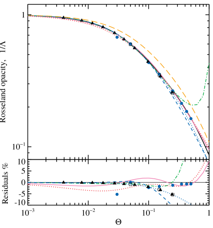
Figure 2: Rosseland mean opacity as a function temperature for non-degenerate gas. Black solid curve represent the result of our exact calculations. The dotted blue curves give the Rosseland mean computed with the help of approximation (23) for the mean free path. The blue circles give the numerical results of Buchler & Yueh (1976), the black triangles are the results from Sampson (1959), and the open squares are from Chin (1965). The dotted red curve is the Paczyński approximation (34), which underestimates exact results by 2–3 %. The solid pink curve is the best fit in the temperature range 2–300 keV using function (40) with parameters $T_{0}=41.5$ keV and $\alpha_{0}=0.9$ which is accurate within 2% in that range. The dashed blue curves is the same approximation in the temperature range 2–40 keV with parameters $T_{0}=39.4$ keV and $\alpha_{0}=0.976$, which is accurate to 0.7%. The dot-dashed green curve is the approximation (32), which is accurate within 3% in the temperature range of 1–150 keV and rapidly diverges at higher temperatures. The long-dashed brown curve represent the flux mean opacity in the free-streaming limit (48) for the blackbody spectrum. The bottom panel presents the residuals in per cent relative to our exact calculations.

The results of calculations for $\Lambda$ in a broad range of temperatures and electron degeneracies $\eta_{-}$ are presented in Figs 2 and 3. We present the results taking opacity by electrons only as was done also by Sampson (1959) and Buchler & Yueh (1976), because at low temperatures or high degeneracy there are no pairs. At low degeneracies and high temperatures $\Theta>-1/\eta$, on the other hand, the number of positrons exceeds the number of electrons, because $\eta_{+}=-2/\Theta-\eta_{-}>\eta_{-}$, which is unphysical. In the following we will replace $\eta_{-}$ by $\eta$. The results computed by Sampson (1959) and Buchler & Yueh (1976) are shown by triangles and circles, respectively, while our results by black solid curves. Results of Sampson (1959) are accurate to better than 1% up to about 25 keV, after that they start to deviate significantly. This is a direct consequence of his usage of approximation (23) for the mean free path, which is supported by our calculations in the same approximation (see dotted blue curves in Figs. 2 and 3b, and the residuals in the bottom panel of Fig. 2). We see that this approximation systematically underestimates the opacity at high temperatures. We note here that the opacity computed by Chin (1965) for degenerate electrons and still reprinted in the textbooks (Weiss et al., 2004) is systematically too large by up to 13% (see black squares in Fig. 3a); a rather good agreement at high temperatures results from a fortuitous cancellation of an error and his usage of approximation (23) (Buchler & Yueh, 1976).

On the other hand, results of Buchler & Yueh (1976) are within 2% from ours above 25 keV ($\Theta>0.05$), but at $\Theta=0.03$ they underestimate the opacity by as much as 6%. The situation becomes worse if we use the analytical approximations of Buchler & Yueh (1976) at lower temperatures, where the opacity would be systematically underestimated by up to 13%.

Calculations of Buchler & Yueh (1976) gave rise to at least two different analytical formulae for the Rosseland mean opacity. Weaver et al. (1978) separated dependencies on $\Theta$ and $\eta$:

$$\Lambda_{\rm W78}(\Theta,\eta)=f_{\Theta}f_{\eta},$$ (32)

where

$$f_{\Theta}=1+14.1\Theta-12.7\Theta^{2}\quad(\mbox{for }\ \Theta<0.4),\qquad f_{\eta}=1+\exp(0.522\eta-1.563).$$ (33)

Expressions (32)–(33) were claimed to be better than 10% accurate in a wide range of degeneracy parameters and temperatures ($-\infty<\eta\lesssim 4$, $0.04<\Theta<0.4$). This approximation is used in the codes developed for simulation of the stellar evolution and explosions, including X-ray bursts (Woosley et al., 2002, 2004). We see (Fig. 3a) it diverges above 150 keV for any $\eta$. Because the dependences on $T$ and $\eta$ are separated, the temperature range of applicability of this approximation becomes smaller for large $\eta$. For $\eta=4$ deviations from the exact values reach 50% in the middle of the temperature range where the approximation suppose to work.

A different approximation that is widely used in theory of X-ray bursts was given by Paczynski (1983):

$$\Lambda_{\rm P83}(\Theta,\eta)=\left[1+\left(\frac{kT}{38.8\,{\rm keV}}\right)^{0.86}\right]\left[1+2.7\times 10^{11}\ \rho\ T^{-2}\right]$$ (34)

for $\mu_{\rm e}=2$. We see from Figs 2 and 3a that Paczyński’s approximation is rather good for small $\eta$. At large $\eta$ it becomes highly inaccurate at low temperatures.

Table 1: Coefficients of the approximate formulae (40) and (35).

	Energy interval of the fit
Coefficient	2–40 keV			2–300 keV
T_0	$39.4$	43.4	$41.5$	43.3
α_0	$0.976$	0.902	$0.90$	0.885
c_01		0.777		0.682
c_02		-0.0509		-0.0454
c_11		0.25		0.24
c_12		-0.0045		0.0043
c_21		0.0264		0.050
c_22		-0.0033		-0.0067
c_31		0.0046		-0.037
c_32		-0.0009		0.0031

         

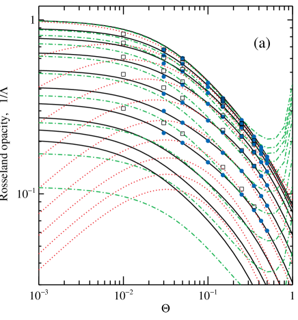
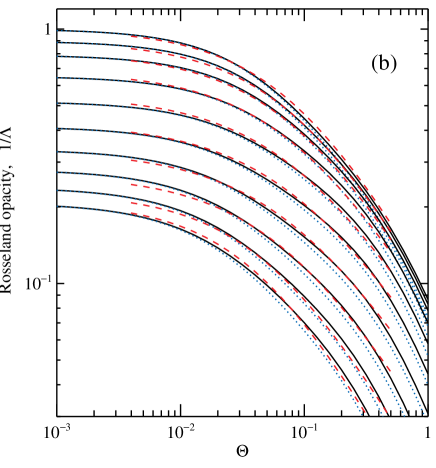
Figure 3: Rosseland mean opacity as a function of temperature for various values of the degeneracy parameter $\eta$. The solid black curves represent the result of our exact calculations (the flux mean opacity is equal to the Rosseland mean within $10^{-4}$). The top curve corresponds to $\eta=-10$, at the following curves $\eta$ varies from $-1$ to $7$. (a) The blue circles give the numerical results of Buchler & Yueh (1976) for $\eta=-10,-1,..,4$ and the black open squares are from Chin (1965) for $\eta=-\infty,-1,0,1,2,4$ (for 5 values of $\Theta$, except for $\eta=-\infty$ for which the opacity is given for only three $\Theta=0.05,0.15,0.25$). The dot-dashed green curves are the approximation (32) and dotted red curves give Paczyński’s approximation (34). (b) The dotted blue curves are the Rosseland mean computed using approximation (23) for the mean free path and the dashed red curves correspond to our approximate expression (35) for the 2–300 keV range.

For the approximation of the Rosseland mean opacity, we propose to use a combination of the forms proposed by Buchler & Yueh (1976) and Paczynski (1983):

$$\Lambda_{\rm app}(\Theta,\eta)=f_{1}(\eta)\left[1+(T/T_{\rm br})^{\alpha}\right],$$ (35)

where

$$T_{\rm br} = T_{0}f_{2}(\eta),$$ (36)

$$\alpha = \alpha_{0}f_{3}(\eta),$$ (37)

$$f_{i}(\eta) = 1+c_{i1}\xi+c_{i2}\xi^{2},\quad i=1,2,3,$$ (38)

$$\xi = \exp(c_{01}\eta+c_{02}\eta^{2}).$$ (39)

The coefficients are given in Table 1 for two fitting intervals 2–40 and 2–300 keV. This form approximates the opacity to better than 4% and 6.5% over the whole range of degeneracy parameter $-10,...,7$ in the temperature ranges 2–40 and 2–300 keV, respectively (see Fig. 3b). In case of a non-degenerate gas, $\eta\rightarrow-\infty$, the expressions simplify as all $f_{i}=1$:

$$\Lambda_{\rm app}(\Theta)=1+(T/T_{0})^{\alpha_{0}},$$ (40)

with the best-fit parameters given in Table 1. The goodness of the fits is demonstrated in Fig. 2. We note, however, that physically realistic parameters should correspond to $N_{-}>N_{+}$, which demands $\Theta<-1/\eta$, i.e. for $\eta=-10$ the temperature is limited by 50 keV.

5 Radiative acceleration and the flux mean opacity

For computation of the radiation force on the medium, we need to construct the first moment of the RKE. Multiplying RKE (14) by $x$ and integrating over ${d}\mbox{\boldmath$x$}$, we get

$$-\mbox{\boldmath$\nabla_{\tau}$}\cdot\mathsf{T}\!=\!\int\!\!\frac{{d}\mbox{\boldmath$x$}}{x}\!\!\int\!\!\frac{{d}\mbox{\boldmath$x$}_{1}}{x_{1}}R(x_{1},x,\mu)n(\mbox{\boldmath$x$})[1+n(\mbox{\boldmath$x$}_{1})]\left(\mbox{\boldmath$x$}-\mbox{\boldmath$x$}_{1}\right),$$ (41)

where we changed the variables $\mbox{\boldmath$x$}\leftrightarrow\mbox{\boldmath$x$}_{1}$ in the second half of the equation and introduced the (dimensionless) radiation pressure tensor

$$\mathsf{T}=\int\ \mbox{\boldmath$x$}\ \mbox{\boldmath$x$}\ n(\mbox{\boldmath$x$})\ \frac{{d}\mbox{\boldmath$x$}}{x}.$$ (42)

This tensor is related to the ordinary radiation pressure tensor as

$$\mathsf{P}=2\frac{m_{\rm e}c^{2}}{\lambda_{\rm C}^{3}}\mathsf{T}.$$ (43)

Let us represent the gradient of the pressure tensor as a sum of the linear and quadratic in $n$ terms:

$$\mbox{\boldmath$\nabla_{\tau}$}\cdot\mathsf{T}=\mbox{\boldmath$\nabla_{\tau}$}\cdot\mathsf{T}_{0}+\mbox{\boldmath$\nabla_{\tau}$}\cdot\mathsf{T}_{1}.$$ (44)

Integrating over angles ${d}^{2}\omega_{1}$, the first term becomes

$$-\mbox{\boldmath$\nabla_{\tau}$}\cdot\mathsf{T}_{0}=\int\frac{{d}\mbox{\boldmath$x$}}{x}\ n(\mbox{\boldmath$x$})\ 4\pi\mbox{\boldmath$\hat{\omega}$}\int_{0}^{\infty}x_{1}\ {d}x_{1}\left[xR_{0}(x_{1},x)-x_{1}R_{1}(x_{1},x)\right]=4\pi\int x^{3}{d}x\ \mbox{\boldmath$h$}_{x}\ [s_{0}(x)-s_{1}(x)]$$ (45)

where

$$\mbox{\boldmath$h$}_{x}=\frac{1}{4\pi}\int\ \mbox{\boldmath$\hat{\omega}$}\ n(\mbox{\boldmath$x$})\ {d}\mbox{\boldmath$\hat{\omega}$}$$ (46)

is the first moment of $n$ and $x[s_{0}(x)-s_{1}(x)]N_{\rm e}\sigma_{\rm T}m_{\rm e}c$ is the momentum transfer per units length of photon propagation averaged over electron distribution and scattered photon directions ignoring induced scattering (Nagirner & Poutanen, 1994; Poutanen & Vurm, 2010; Pozdnyakov et al., 1983). Note the radiation flux in these notations is

$$\mbox{\boldmath$F$}\propto\int x^{3}{d}x\ \mbox{\boldmath$h$}_{x}\ .$$ (47)

Thus the flux mean opacity (in units of $N_{\rm e}\sigma_{\rm T}/\rho$) in the free streaming limit (ignoring induced scattering) is

$$\kappa_{\rm F}=\frac{\int x^{3}{d}x\ h_{x}\ [s_{0}(x)-s_{1}(x)]}{\int x^{3}{d}x\ h_{x}}.$$ (48)

For the radiation spectrum close to the diluted blackbody, i.e. $h_{x}\propto b_{x}$, the flux mean opacity for the case of non-degenerate electrons is shown in Fig. 2. Eq. (40) with parameters $T_{0}=58.5$ keV and $\alpha_{0}=0.913$ provides a good approximation with better than 0.8% accuracy to the corresponding mean free path in the 2–300 keV range.

In the diffusion approximation (15), we substitute $\mbox{\boldmath$h$}_{x}=-\frac{1}{3}l_{x}\mbox{\boldmath$\nabla_{\tau}$}b_{x}$. The effect of the induced scattering on the radiation pressure force in the diffusion approximation can be computed by substituting equation (15) to Eq. (41). The non-linear term becomes:

$$-\mbox{\boldmath$\nabla_{\tau}$}\cdot\mathsf{T}_{1}=\int x{d}x\int x_{1}{d}x_{1}\int{d}^{2}\omega\int{d}^{2}\omega_{1}\left(b_{x}+\eta l_{x}\partial_{\tau}b_{x}\right)\left(b_{x_{1}}+\eta_{1}l_{x_{1}}\partial_{\tau}b_{x_{1}}\right)R(x_{1},x,\mu)\left(x\mbox{\boldmath$\hat{\omega}$}-x_{1}\mbox{\boldmath$\hat{\omega}$}_{1}\right),$$ (49)

where $\mbox{\boldmath$\hat{\omega}$}=(\sqrt{1-\eta^{2}}\cos\phi,\sqrt{1-\eta^{2}}\sin\phi,\eta)$ and $\mbox{\boldmath$\hat{\omega}$}_{1}=(\sqrt{1-\eta_{1}^{2}}\cos\phi_{1},\sqrt{1-\eta_{1}^{2}}\sin\phi_{1},\eta_{1})$ with the $z$-axis chosen against the temperature gradient and $\partial_{\tau}b_{x}\equiv|\mbox{\boldmath$\nabla_{\tau}$}b_{x}|$. Taking the angular integrals, for the magnitude of the radiation pressure force we get

$$\!\!-|\mbox{\boldmath$\nabla_{\tau}$}\cdot\mathsf{T}_{1}|=\frac{16\pi^{2}}{3}\!\!\int\!\!x{d}x\!\!\int\!\!x_{1}{d}x_{1}\left[R_{0}(x_{1},x)\left(b_{x_{1}}xl_{x}\partial_{\tau}b_{x}-b_{x}x_{1}l_{x_{1}}\partial_{\tau}b_{x_{1}}\right)+R_{1}(x_{1},x)\left(xb_{x}l_{x_{1}}\partial_{\tau}b_{x_{1}}-x_{1}b_{x_{1}}l_{x}\partial_{\tau}b_{x}\right)\right].$$ (50)

Making variable change $x\leftrightarrow x_{1}$ in the terms containing $\partial_{\tau}b_{x_{1}}$, we get

$$-|\mbox{\boldmath$\nabla_{\tau}$}\cdot\mathsf{T}_{1}|=\frac{16\pi^{2}}{3}\int\!\!x{d}x\ l_{x}\partial_{\tau}b_{x}\!\!\int\!\!x_{1}{d}x_{1}b_{x_{1}}\left\{\left[xR_{0}(x_{1},x)-x_{1}R_{1}(x_{1},x)\right]-\left[xR_{0}(x,x_{1})-x_{1}R_{1}(x,x_{1})\right]\right\}.$$ (51)

The total pressure gradient becomes

$$\!\!\!\!\!\!-|\mbox{\boldmath$\nabla_{\tau}$}\cdot\mathsf{T}| = \frac{16\pi^{2}}{3}\int x{d}x\ l_{x}\partial_{\tau}b_{x}\int x_{1}{d}x_{1}\left\{(1+b_{x_{1}})\left[xR_{0}(x_{1},x)-x_{1}R_{1}(x_{1},x)\right]-b_{x_{1}}\left[xR_{0}(x,x_{1})-x_{1}R_{1}(x,x_{1})\right]\right\}$$ (52)

$$= \frac{16\pi^{2}}{3}\!\!\!\int\!\!x{d}x\ l_{x}\partial_{\tau}b_{x}\int\!\!x_{1}{d}x_{1}\frac{1-e^{-x/\Theta}}{1-e^{-x_{1}/\Theta}}\left[xR_{0}(x_{1},x)-x_{1}R_{1}(x_{1},x)\right]=\frac{4\pi}{3}\!\!\int\!\!x^{3}{d}x\ l_{x}\partial_{\tau}b_{x}\left[r_{0}(x)-r_{1}(x)\right].$$

Thus the flux mean opacity is then

$$\kappa_{\rm F}=\frac{\displaystyle\int_{0}^{\infty}l_{x}\ [r_{0}(x)-r_{1}(x)]\frac{\partial B_{x}}{\partial\Theta}{d}x}{\displaystyle\int_{0}^{\infty}l_{x}\frac{\partial B_{x}}{\partial\Theta}{d}x}.$$ (53)

Because approximation (25), i.e. $1/l_{x}\approx r_{0}(x)-r_{1}(x)$, is very accurate in the region of the photon energies $x\sim\Theta$ contributing to the integral, the flux mean opacity in the diffusion approximation turned out to be nearly identical (with the relative difference less than $10^{-4}$) to the Rosseland mean in the full range of considered temperatures and degeneracies. The flux mean opacity thus can be approximated by simple analytical expressions (35) and (40), which also describe well the radiative acceleration in the atmospheres of hot neutron stars obtained from the solution of the radiative transfer equation with the exact Compton redistribution function where diffusion approximation has not been used (Suleimanov et al., 2012).

6 Summary

In this paper, we have critically evaluated results of previous works on the Rosseland mean opacity for Compton scattering. In order to obtain the photon mean free path as a function of photon energy we have solved relativistic kinetic equation describing photon interactions via Compton scattering with the possibly degenerate electron gas. We demonstrated that the mean free path can be also accurately evaluated using explicit approximate formulae, which can also be used for calculations of the Rosseland mean opacity and can provide a simple way for accounting for the true absorption.

We have computed the Rosseland and the flux mean opacities (which are nearly identical in the diffusion approximation) in a broad range of temperatures and electron degeneracy parameter. We compared our results to the previous calculations and found significant difference in the low-temperature regime. We have also presented useful analytical expressions that approximate well the numerical results.

Appendix A Redistribution functions

In case of non-degenerate electrons, the RF defined by Eq. (11) has been studied in details before (Aharonian & Atoyan, 1981; Prasad et al., 1986; Nagirner & Poutanen, 1994; Poutanen & Vurm, 2010). This RF can be simplified to the one-dimentional integral over the electron energy. For degenerate electrons, it turned out that the derivation is identical and also in this case, the RF can be presented in terms of one integral that can be taken numerically.

For the isotropic electron distribution expression (11) for the RF can be simplified by taking the integral over $p$ with the help of the 3-dimensional delta-function and using the identity $\delta(\gamma_{1}+x_{1}-\gamma-x)=\gamma\delta\left(\underline{x}_{1}\cdot\underline{p}_{1}-\underline{x}\cdot(\underline{p}_{1}+\underline{x}_{1})\right)$:

$$R_{\pm}(x,x_{1},\mu)=\frac{3}{16\pi}\frac{2}{\lambda_{\rm C}^{3}N_{\pm}}\!\!\int\!\!\frac{{d}\mbox{\boldmath$p$}_{1}}{\gamma_{1}}\tilde{n}_{\pm}(\gamma_{1})[1-\tilde{n}_{\pm}(\gamma)]F\delta(\Gamma),$$ (A1)

where

$$\gamma = \gamma_{1}+x_{1}-x,$$ (A2)

$$\Gamma = \gamma_{1}(x_{1}-x)-p_{1}(x_{1}\mbox{\boldmath$\hat{\omega}$}_{1}-x\mbox{\boldmath$\hat{\omega}$})\cdot\mbox{\boldmath$\hat{\Omega}$}_{1}-q,$$ (A3)

$$q = \mbox{\boldmath$x$}\cdot\mbox{\boldmath$x$}_{1}=xx_{1}(1-\mu).$$ (A4)

The RF depends also implicitly on the electron temperature $\Theta$ and degeneracy parameter $\eta_{\pm}$. To integrate over angles in Eq. (A1) we follow the recipe proposed by Aharonian & Atoyan (1981) (see also Prasad et al. 1986; Poutanen & Vurm 2010), choosing the polar axis along the direction of the transferred momentum

$$\mbox{\boldmath$\hat{n}$}\equiv\left(x_{1}\mbox{\boldmath$\hat{\omega}$}_{1}-x\mbox{\boldmath$\hat{\omega}$}\right)/Q,$$ (A5)

where

$$Q^{2}=(x_{1}\mbox{\boldmath$\hat{\omega}$}_{1}-x\mbox{\boldmath$\hat{\omega}$})^{2}=(x-x_{1})^{2}+2q.$$ (A6)

Thus the integration variables become $\cos\alpha=\mbox{\boldmath$\hat{n}$}\cdot\mbox{\boldmath$\hat{\Omega}$}_{1}$ and the corresponding azimuth $\Phi$. The RF (A1) then can be written as

$$R_{\pm}(x,x_{1},\mu)=\frac{3}{16\ \pi}\frac{2}{\lambda_{\rm C}^{3}N_{\pm}}\!\int\limits_{1}^{\infty}\!\!\,\tilde{n}_{\pm}(\gamma_{1})[1-\tilde{n}_{\pm}(\gamma)]p_{1}{d}\gamma_{1}\int\limits_{-1}^{1}\!\!\,\delta(\Gamma)\ {d}\cos\alpha\!\!\int\limits_{0}^{2\pi}\!\!\,F{d}\Phi,$$ (A7)

where now

$$\Gamma=\gamma_{1}(x_{1}-x)-q-p_{1}Q\cos\alpha.$$ (A8)

Integrating over $\cos\alpha$ using the delta-function we get

$$R_{\pm}(x,x_{1},\mu)=\frac{3}{8}\frac{2}{\lambda_{\rm C}^{3}N_{\pm}}\int_{\gamma_{*}}^{\infty}\!\!\tilde{n}_{\pm}(\gamma_{1})[1-\tilde{n}_{\pm}(\gamma)]\ R(x,x_{1},\mu,\gamma_{1})\ {d}\gamma_{1},$$ (A9)

with integration over the electron distribution done numerically. Here we introduced the RF for monoenergetic electrons

$$R(x,x_{1},\mu,\gamma_{1})=\frac{1}{Q}\frac{1}{2\pi}\int_{0}^{2\pi}\>F\ {d}\Phi.$$ (A10)

Function $F$ depends on $\xi_{1}=x(\gamma_{1}-p_{1}\zeta)$ and $\xi=\xi_{1}+q$, where

$$\zeta = \mbox{\boldmath$\hat{\omega}$}\cdot\mbox{\boldmath$\hat{\Omega}$}_{1}=\cos\alpha\cos\kappa+\sin\alpha\sin\kappa\cos\Phi,$$ (A11)

$$\cos\alpha = \mbox{\boldmath$\hat{n}$}\cdot\mbox{\boldmath$\hat{\Omega}$}_{1}=\left[\gamma_{1}(x_{1}-x)-q\right]/p_{1}Q,$$ (A12)

$$\cos\kappa = \mbox{\boldmath$\hat{\omega}$}\cdot\mbox{\boldmath$\hat{n}$}=(x_{1}\mu-x)/Q,$$ (A13)

The condition $|\cos\alpha|\leq 1$, gives a constraint

$$\gamma_{1}\geq\gamma_{*}(x,x_{1},\mu)=\left(x-x_{1}+Q\sqrt{1+2/q}\right)/2.$$ (A14)

Integrating over azimuth $\Phi$ in Eq. (A10) gives the exact analytical expression for the RF valid for any photon and electron energy (Buchler & Yueh, 1976; Aharonian & Atoyan, 1981; Prasad et al., 1986; Nagirner & Poutanen, 1994; Poutanen & Vurm, 2010), which we use in our calculations:

$$R(x,x_{1},\mu,\gamma_{1})\!=\!\frac{2}{Q}+\frac{q^{2}-2q-2}{q^{2}}\left(\frac{1}{a_{-}}\!-\!\frac{1}{a_{+}}\right)+\frac{1}{q^{2}}\left(\frac{d_{-}}{a_{-}^{3}}\!+\!\frac{d_{+}}{a_{+}^{3}}\right),$$ (A15)

where

$$a_{-}^{2}=(\gamma_{1}-x)^{2}+\frac{1+\mu}{1-\mu},\quad a_{+}^{2}=(\gamma_{1}+x_{1})^{2}+\frac{1+\mu}{1-\mu},\quad d_{\pm}=\left(a_{+}^{2}-a_{-}^{2}\pm Q^{2}\right)/2.$$ (A16)

The cancellations at small photon energies has been handled by Nagirner & Poutanen (1993). We note that the RF (A10) satisfies the detailed balance condition (Nagirner & Poutanen, 1994):

$$R(x,x_{1},\mu,\gamma_{1})=R(x_{1},x,\mu,\gamma_{1}+x_{1}-x).$$ (A17)

The RF (A1) is related to the scattering kernel (8.13) in Pomraning (1973) as $R(x,x_{1},\mu)=\sigma_{s}(x_{1}\rightarrow x,\mu)x_{1}/x$. The form given by Eq. (A7) is equivalent to eq. (A4) in Buchler & Yueh (1976). The derived RF for monoenergetic electrons (A15) is equivalent to eq. (A5) from Buchler & Yueh (1976) and eq. (14) in Aharonian & Atoyan (1981).

The angle-averaged RF functions (19) and (20), used in the calculations of the mean free path, can be expressed through the single integral over the electron and positron distributions

$$R_{i}(x,x_{1})=\frac{3}{16}\frac{2}{\lambda_{\rm C}^{3}N_{\rm e}}\int_{\gamma^{\prime}_{\star}}^{\infty}R_{i}(x,x_{1},\gamma_{1})\ {d}\gamma_{1}\left\{\tilde{n}_{-}(\gamma_{1})[1-\tilde{n}_{-}(\gamma)]+\tilde{n}_{+}(\gamma_{1})[1-\tilde{n}_{+}(\gamma)]\right\},\quad i=0,1,$$

where

$$\gamma^{\prime}_{\star}(x,x_{1})\!\!=\!\!\left\{\begin{array}[]{ll}\displaystyle\frac{x-x_{1}}{2}+\frac{x+x_{1}}{2}\!\!\sqrt{1+\!\!\frac{1}{xx_{1}}}&\mbox{if $|x-x_{1}|\geq 2xx_{1}$,}\\ 1+\left(x-x_{1}+|x-x_{1}|\right)/2&\mbox{if $|x-x_{1}|\leq 2xx_{1}$.}\end{array}\right.$$ (A18)

The explicit analytical expressions for the angle-integrated functions $R_{0}(x,x_{1},\gamma_{1})$ and $R_{0}-R_{1}$ under the integrals in Eqs. (A) can be found in sections 8.1 and 8.2 of Nagirner & Poutanen (1994).

References

- Aharonian & Atoyan (1981) Aharonian, F. A. & Atoyan, A. M. 1981, Ap&SS, 79, 321
- Berestetskii et al. (1982) Berestetskii, V. B., Lifshitz, E. M., & Pitaevskii, V. B. 1982, Quantum electrodynamics (Oxford: Pergamon Press)
- Buchler & Yueh (1976) Buchler, J. R. & Yueh, W. R. 1976, ApJ, 210, 440
- Chin (1965) Chin, C.-W. 1965, ApJ, 142, 1481
- Chiu (1968) Chiu, H.-Y. 1968, Stellar physics. Vol.1 (Blaisdell: Waltham, Mass.)
- Cox & Giuli (1968) Cox, J. P. & Giuli, R. T. 1968, Principles of stellar structure (New York: Gordon and Breach)
- de Groot et al. (1980) de Groot, S. R., van Leeuwen, W. A., & van Weert, C. G. 1980, Relativistic kinetic equation (Amsterdam: North-Holland)
- Mihalas & Mihalas (1984) Mihalas, D. & Mihalas, B. W. 1984, Foundations of radiation hydrodynamics (New York: Oxford University Press)
- Nagirner & Poutanen (1993) Nagirner, D. I. & Poutanen, J. 1993, A&A, 275, 325
- Nagirner & Poutanen (1994) —. 1994, Single Compton scattering, Vol. 9 (Amsterdam: Harwood Academic Publishers), 1–83
- Paczynski (1983) Paczynski, B. 1983, ApJ, 267, 315
- Pomraning (1973) Pomraning, G. C. 1973, The equations of radiation hydrodynamics (Oxford: Pergamon Press)
- Poutanen & Vurm (2010) Poutanen, J. & Vurm, I. 2010, ApJS, 189, 286
- Pozdnyakov et al. (1983) Pozdnyakov, L. A., Sobol, I. M., & Syunyaev, R. A. 1983, Astrophysics and Space Physics Reviews, 2, 189
- Prasad et al. (1986) Prasad, M. K., Kershaw, D. S., & Beason, J. D. 1986, Appl. Phys. Lett., 48, 1193
- Sampson (1959) Sampson, D. H. 1959, ApJ, 129, 734
- Suleimanov et al. (2012) Suleimanov, V., Poutanen, J., & Werner, K. 2012, A&A, 545, A120
- Weaver et al. (1978) Weaver, T. A., Zimmerman, G. B., & Woosley, S. E. 1978, ApJ, 225, 1021
- Weiss et al. (2004) Weiss, A., Hillebrandt, W., Thomas, H.-C., & Ritter, H. 2004, Cox and Giuli’s Principles of Stellar Structure (Cambridge: Princeton Publishing Associates Ltd)
- Woosley et al. (2004) Woosley, S. E., Heger, A., Cumming, A., Hoffman, R. D., Pruet, J., Rauscher, T., Fisker, J. L., Schatz, H., Brown, B. A., & Wiescher, M. 2004, ApJS, 151, 75
- Woosley et al. (2002) Woosley, S. E., Heger, A., & Weaver, T. A. 2002, Reviews of Modern Physics, 74, 1015