Vote-boosting ensembles

Abstract

Vote-boosting is a sequential ensemble learning method in which the individual classifiers are built on different weighted versions of the training data. To build a new classifier, the weight of each training instance is determined in terms of the degree of disagreement among the current ensemble predictions for that instance. For low class-label noise levels, especially when simple base learners are used, emphasis should be made on instances for which the disagreement rate is high. When more flexible classifiers are used and as the noise level increases, the emphasis on these uncertain instances should be reduced. In fact, at sufficiently high levels of class-label noise, the focus should be on instances on which the ensemble classifiers agree. The optimal type of emphasis can be automatically determined using cross-validation. An extensive empirical analysis using the beta distribution as emphasis function illustrates that vote-boosting is an effective method to generate ensembles that are both accurate and robust.

1 Introduction

In ensemble learning, the outputs of a collection of diverse classifiers are combined to exploit their complementarity, in the expectation that the global ensemble prediction be more accurate than the individual ones [14]. The complementarity of the classifiers is either an indirect consequence of diversity, as in bagging [7] and random forests [11], or can be explicitly favored by design, as in negative correlation learning [34] and boosting [47, 22, 23, 48]. In this manuscript, we present vote-boosting, an ensemble learning method of the latter type, in which the progressive focus on a particular training instance depends on the degree of disagreement among the predictions of the ensemble classifiers. By contrast to standard boosting algorithms, the strength of this emphasis is independent of whether the instance is correctly or incorrectly classified. The optimal emphasis profile depends on the characteristics of the classification problem considered and on the complexity of the base learners. In problems with no or low levels of noise in the class labels of the training instances the appropriate focus is on instances on which the classifiers disagree (i.e. instances for which the ensemble prediction has a high degree of uncertainty). As the noise level increases, especially when more flexible base learners (e.g. unpruned CART or random trees) are used, the emphasis on uncertain instances should be reduced. In fact, in problems with sufficiently high levels of class-label noise, the optimal strategy is to assign larger weights to instances on which the ensemble classifiers agree. In practice, the determination of the optimal emphasis strategy can be automatically made through parameter selection (e.g. though cross-validation on the training data). The results of an extensive empirical will be used to illustrate that vote-boosting is an effective method to build accurate ensembles that are both accurate and robust to class-label noise.

The article is organized as follows: In Section 2, we provide a review of ensemble methods that are related to the current proposal. Vote-boosting is described in section 3. In this section, we show that the ensemble construction algorithm can be viewed as an optimization by gradient descent in the functional space of linear combinations of hypothesis. In Section 4, the properties and performance of vote-boosting ensembles are analyzed in an extensive empirical evaluation on synthetic and real-world classification tasks from different domains of application. Finally, the conclusions of this study are summarized in Section 5.

2 Previous Work

There are a wide variety of methods to build ensembles. In this work, we focus on homogeneous ensembles, which are composed of predictors of the same type. Each of the predictors in the ensemble is built from a training set composed of labeled instances. Once the individual predictors have been built, their outputs are combined to reach a global ensemble decision. A wide range of alternatives can be used to carry out this combination [53]. Nevertheless, simple strategies, such as averaging real-valued outputs, or majority voting, if the individual classifiers yield class-labels, are generally effective [24].

Randomization techniques can be used to generate collections of diverse classifiers. The objective is to build predictors whose errors are as independent as possible. If these errors of these classifiers are independent, they can be averaged out by the combination process. An example of these types of ensembles is bagging [7]. The individual classifiers in a bagging ensemble are built by applying a fixed learning algorithm to independent bootstrap samples drawn from the original training data. In class-switching ensembles, each member is built using a perturbed versions of the original training set, in which the class labels of a fraction of instances are modified at random [10, 38]. Alternatively, diverse classifiers can be built by including some randomized steps in the learning algorithm itself. For instance, in one of the earliest works on ensembles of neural networks [29], one takes advantage of the presence of multiple local minima in the optimization process that is used to tune the synaptic weights and averages over the predictions of the neural networks that result from different initializations. Random forests [11], which are one of the most effective ensemble methods [17], are built using a combination of data randomization and randomization in the learning algorithm: The ensemble classifiers are random trees, which are trained on bootstrap replicates of the original training dataset. Other effective classifiers of this type are rotation forests [46] and ensembles of extremely randomized trees [25].

An alternative to simply generating diversity is to explicitly aim to increase the complementarity of the enseble classifiers. An example of this strategy is Negative Correlation Learning [34]. In this method, complementarity is favored by simultaneously training all the classifiers in the ensemble: The parameters of the individual classifiers and the weights for the combination of their outputs are determined globally by minimizing a cost function that penalizes coincident predictions. Another example is boosting. Boosting originally refers to the problem of building a strong learner out of a collection of weak learners; i.e. learners whose predictive accuracy is only slightly better than random guessing [47, 23, 48]. AdaBoost is one of the most widely used boosting algorithms [22]. In AdaBoost an ensemble is grown by incorporating classifiers that progressively focus on instances that are misclassified by the previous classifiers in the sequence. The individual classifiers are built by applying a learning algorithm that can handle individual instance weights. Alternatively, weighted resampling in the training set can be used. The first classifier is obtained by assuming equal weights for all instances. The subsequent classifiers are built using different emphasis on each of the training instances. Specifically, to build the $t$-th classifier in the sequence, the weights of instances that are misclassified by the most recent classifier in the ensemble are increased. Correspondingly, the weights of the correctly classified instances are reduced. The final prediction of the ensemble is determined by weighted majority voting. The weight of an individual classifier in the final ensemble prediction depends on the weighted accuracy of this classifier on the training set. The margin of an instance is defined as the sum of weighted votes for the correct class minus the sum of weighted votes for the most voted incorrect class. Therefore, misclassified instances have negative margins. In AdaBoost, the evolution of the weight of a particular instance is a monotonically decreasing function of its margin [21].

AdaBoost is one of the most effective ensemble methods [15, 37, 17]. However, it is not robust to class-label noise [44, 5, 32]. Specifically, AdaBoost gives unduly high weights to noisy instances, whose class labels are incorrect. There are numerous studies that address this excessive sensitivity of AdaBoost to class-label noise [36, 1, 16, 31, 26, 50, 23, 45, 28, 51, 52, 19, 20, 12]. A possible strategy is to identify and either remove noisy instances in the training data, or correct their class-labels [36, 1]. Another alternative is to apply explicit or implicit regularization techniques to avoid assigning excessive weight to a reduced group of instances [16, 31, 26, 40, 50]. For instance, the logistic loss function employed in LogitBoost [23] gives less emphasis to instances with large negative margins than the exponential loss function used in AdaBoost. In consequence, LogitBoost is generally more robust to class-label noise [41]. In other studies, penalty terms are used in the cost function to avoid focusing on outliers or on instances that are difficult to classify [45, 28, 51, 52]. It is possible to also use hybrid weighting methods that modulate the emphasis on instances according to their distance to the decision boundary [27, 26, 2]. Most boosting algorithms use convex loss functions. This has the advantage that the resulting optimization problem can be solved efficiently using, for instance, gradient descent. However, as shown in [35], the generalization capacity of boosting variants that use convex loss functions can be severely affected by class-label noise. Alternative non-convex loss functions are used in BrownBoost and other robust boosting variants [19, 20, 12]. In these methods, the evolution of the weights is not a monotonic function of the margin: instances with small negative margins (i.e. misclassified instances that are close to the decision boundary) are assigned higher weights, as in AdaBoost. However, instances whose margin is negative and large receive lower weights. The rationale for using this type of emphasis is that instances in regions with a large class overlap tend to have small margins. Focusing on these instances is beneficial because the classification boundary can be modeled in more detail. By contrast, large negative margins correspond to misclassified instances that are far from the classification boundary. A robust boosting algorithm should therefore avoid emphasizing these instances, which are likely to be noisy.

In the next section we introduce vote-boosting, a novel boosting algorithm in which the weights of the instances are determined in terms of the degree of agreement or disagreement among the predictions of the ensemble members, irrespective of their actual class labels. As illustrated by the results of empirical evaluation presented in section 4, the optimal type of emphasis (that is, whether the focus should be placed on instances on which the classifiers disagree, or on instances on which they agree) can be determined from the training data alone using, for instance, cross-validation. Since the instance weights do not depend on whether the predictions by the ensemble classifiers are correct, it is possible to avoid unduly emphasizing incorrectly classified instances that are outliers, which is one of the weaknesses of standard boosting algorithms, such as AdaBoost. In this manner, one can build accurate ensembles that are robust to class-label nosie.

3 Vote-boosting

Consider the problem of automatic induction of a classification system from labeled training data. The original training set is composed of $N_{train}$ attribute class-label pairs $\mathcal{D}_{train}=\left\{\left(\mathbf{x}_{i},y_{i}\right)\right\}_{i=1}^{N_{train}}$, where ${\mathbf{x}}\in\mathcal{X}$. In this article, we focus on binary classification tasks, in which $y\in\{-1,1\}$. Problems with multiple classes can be addressed with a number of strategies, such as the ones used in combination with AdaBoost for this purpose [48].

Let $\left\{f_{\tau}(\cdot)\right\}_{\tau=1}^{t}$ be a partially-grown ensemble of size $t$. The $\tau$-th classifier in the ensemble is a function $f_{\tau}:\mathbb{R}^{D}\rightarrow\{-1,1\}$ that maps a vector of attributes $\mathbf{x}$ to a class label $f_{\tau}(\mathbf{x})$. This function is obtained by applying a base learning algorithm to a training set, taking into account the individual instance weights $\left\{w_{i}^{[\tau]}\right\}_{i=1}^{N_{train}}$.

To obtain the prediction of the ensemble, the predictions of the individual classifiers are aggregated by weighted averaging

$$F_{t}(\mathbf{x})=\sum_{\tau=1}^{t}\alpha_{\tau}^{[t]}f_{\tau}(\mathbf{x}),\quad F_{t}\in\left\{-1,1\right\},$$ (1)

where $\alpha_{\tau}^{[t]}\geq 0$ is the weight of the prediction of the $\tau$ classifier. These weights are normalized $\sum_{\tau=1}^{t}\alpha_{\tau}=1$. In (unweighted) majority voting one assumes that all the predictions have the same weight , $\alpha_{\tau}^{[t]}=1/t$. This simple voting scheme provides good overall results. For this reason, it will be used in our implementation. Based on this aggregated output, the final prediction of the ensemble of size $t$ is

$$H_{t}(\mathbf{x})=sign\left(F_{t}(\mathbf{x})\right).$$ (2)

Assuming that $t$ is odd, $H_{t}(\mathbf{x})\in\left\{-1,1\right\}$. At this stage of the ensemble construction process, instance $\mathbf{x}$ can be characterized by $t_{+}(\mathbf{x})$ and $t_{-}(\mathbf{x})=t-t_{+}(\mathbf{x})$, the counts of positive and negative votes, respectively. The fractions of votes in each class are

$$\pi^{[t]}_{\pm}(\mathbf{x})=\frac{t_{\pm}(\mathbf{x})}{t};\quad\pi^{[t]}_{+}(\mathbf{x})+\pi^{[t]}_{-}(\mathbf{x})=1.$$ (3)

These values can be used to quantify the level of certainty of the ensemble prediction. Values $\pi^{[t]}_{+}(\mathbf{x})$ close to $0$ or $1$ correspond to instances for which the predictions of most ensemble classifiers coincide. Instances whose classification by the ensemble is uncertain are characterized by $\pi^{[t]}_{+}(\mathbf{x})$ close to $1/2$. In contrast to standard boosting algorithms, in vote-boosting, the instance weights depend on the degree of agreement or disagreement among the predictions of the individual classifiers, not on whether these predictions are erroneous.

The pseudo-code of the proposed vote-boosting algorithm is presented in Figure 1.

Input:

$\quad\mathcal{D}_{train}=\left\{\left(\mathbf{x}_{i},y_{i}\right)\right\}_{i=1}^{N_{train}},\ \mathbf{x}_{i}\in\mathcal{X},\ y_{i}\in\{-1,1\}$

$\quad T$ % Ensemble size

$\quad\mathcal{L}$ % Base learning algorithm

$\quad g(p)$ % Non-negative emphasis function ($0\leq p\leq 1$)

1 $F_{0}(\cdot)\leftarrow 0$

2$t_{+}(\mathbf{x}_{i})\leftarrow 0$ $\forall i=1,...,N_{train}$

3$w_{i}^{[1]}\leftarrow\frac{1}{N_{train}}$ $\forall i=1,...,N_{train}$

4 for $t\leftarrow 1$ to $T$ do

5       $f_{t}(\cdot)\leftarrow\mathcal{L}\left(\mathcal{D}_{train},\mathbf{w}^{[t]}\right)$

6       $t_{+}(\mathbf{x}_{i})\leftarrow t_{+}(\mathbf{x}_{i})+\mathbb{I}(f_{t}(\mathbf{x}_{i})>0)$ $\forall i=1,...,N_{train}$

7       $\pi_{+}(\mathbf{x}_{i})=\frac{t_{+}(\mathbf{x}_{i})+1}{t+2}$ $\forall i=1,...,N_{train}$

8       $w_{i}^{[t+1]}\leftarrow g\left(\pi_{+}(\mathbf{x}_{i})\right)$ $\forall i=1,...,N_{train}$

9       Normalize $\mathbf{w}^{[t]}$

10       $F_{t}(\cdot)\leftarrow F_{t-1}(\cdot)+f_{t}(\cdot)$

11      

Output: $H_{T}(\cdot)=sign(F_{T}(\cdot))$

Algorithm 1 Vote-boosting algorithm with resampling

The final ensemble is composed of $T$ classifiers, each of which is built by applying the base learning algorithm $\mathcal{L}$ on the training data with different sets of instance weights. The weights of the instances can be taken into account using weighted resampling with replacement

$$\mathcal{D}_{train}^{[t]} = \text{Sample}\left(\mathcal{D}_{train},\mathbf{w}^{[t]}\right)$$

$$f_{t} \leftarrow \mathcal{L}\left(\mathcal{D}_{train}^{[t]}\right).$$ (4)

For the induction of the first ensemble classifier all instances are assigned the same weight. These weights are updated at each iteration according to the tally of votes: Assuming that instance $\mathbf{x}_{i}$ has received $t_{+}\left(\mathbf{x}_{i}\right)$ votes for the positive class at the $t$-th iteration, we use the Laplace estimator of the probability that a classifier in the ensemble outputs a particular class prediction

$$\pi_{\pm}(\mathbf{x}_{i})=\frac{t_{\pm}(\mathbf{x}_{i})+1}{t+2}.$$ (5)

Finally the weights are updated

$$w_{i}^{[t+1]}=\frac{1}{\mathcal{Z}_{t+1}}g\left(\pi_{+}(\mathbf{x}_{i})\right),\quad\text{for}\;\;i=1,...,N_{train},$$ (6)

where $g:[0,1]\rightarrow\mathbb{R}^{+}$ is an emphasis function, which is non-negative, and

$$\mathcal{Z}_{t+1}=\sum_{i=1}^{N_{train}}g\left(\pi_{+}(\mathbf{x}_{i})\right)$$ (7)

is a normalization constant. These weights are then used to build the following classifier in the ensemble.

A natural choice for the emphasis function is the probability density of the beta distribution with shape parameters $a$, $b$

$$g(p)\equiv\beta\left(p;a,b\right)=\frac{\Gamma(a+b)}{\Gamma(a)\Gamma(b)}p^{a-1}(1-p)^{b-1},\quad 0\leq p\leq 1.$$ (8)

For this particular emphasis function, the weights at the $(t+1)$-th iteration are updated according to

$$w_{i}^{[t+1]}=\frac{1}{Z_{t+1}}\beta\left(\pi_{+}(\mathbf{x}_{i});a,b\right)$$ (9)

If the class distributions are not strongly imbalanced, the choice $a=b$, in which the two classes are handled in a symmetrical manner, is generally appropriate. In problems with a large class imbalance, an asymmetric choice of the emphasis function may be preferable. In Figure 1 the density profiles of the symmetric beta distribution for different values of $a$=$b\in\{0.25,0.75,1,1.5,2.5,5,10,20,40\}$ are shown. If $a=b=1$, the distribution is uniform. Therefore, all instances are given the same importance (plot in the first row, third column of Figure 1). In this case, the proposed algorithm is equivalent to bagging [7]. For $a=b>1$ the distribution becomes unimodal, with a maximum at $0.5$. In this range, the higher the values of $a=b$, the more concentrated becomes the probability around the mode. In consequence, vote-boosting emphasizes uncertain instances and reduces the importance of those instances on which most classifiers agree. For simple classifiers, the emphasis on uncertain instances that one obtains is similar to the error-based emphasis of AdaBoost. The reason is that uncertain instances are generally more difficult to classify and, in consequence, are more likely to be incorrectly classified. In the regime $a=b<1.0$, vote boosting progressively focuses on instances that are far from the classification boundary. As will be illustrated in the section on experiments, this strategy is effective in complex or noisy problems, especially when the ensemble is composed of flexible classifiers, because of its regularizing effects.

Figure 1: Symmetric beta distribution with $a=b=[0.25,0.75,1,1.5,2.5,5,10,20,40]$

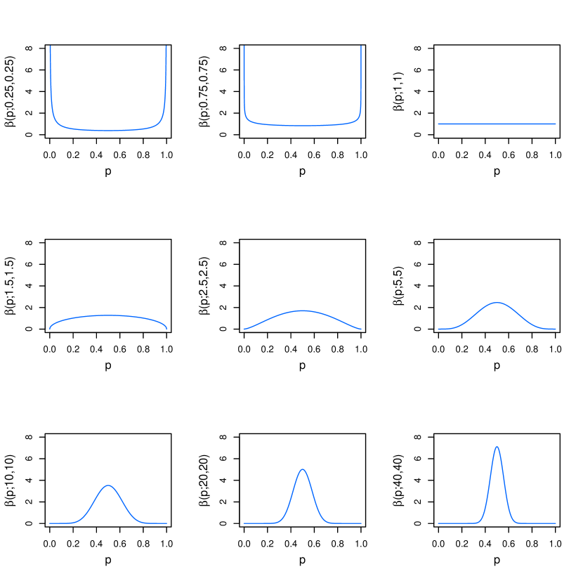
It is common, especially in the first iterations of the algorithm, when the ensemble is still small, that all the classifiers predict the same class label for some instances. In such cases, the fraction of positive votes is either $0$ or $1$. Except for $a=b=1$, the value of the beta distribution at these points is either zero or infinity. In the case of zero density values, those instances would be assigned zero weight in the next iteration of the algorithm. Thus, they would be effectively removed from the sample. In the other extreme, some instances would have infinite weights. To avoid these evaluations of the beta distribution at the boundaries of its support, the Laplace correction has been used in the estimation of class prediction probabilities (5).

Finally, we note that vote-boosting can be used with base learners that achieve zero or low error rates in the training data. In such cases, the weights that AdaBoost assigns to the training instances are ill-defined. By contrast, even if the training error of a single ensemble classifier is zero or close to zero, there can be disagreement among the individual predictions. Therefore, provided that the Laplace correction is used in the estimation of class prediction probabilities, the weights given by Eq. 9, are always well defined. This feature allows us to build vote-boosting ensembles of unpruned CART or random trees, which, as illustrated by the results of Section 4 are both accurate and robust to class-label noise.

3.1 A functional gradient interpretation of vote-boosting

Similarly to other boosting methods, vote-boosting can be viewed as a gradient descent algorithm in the hypothesis space of linear combinations of predictors [39]. Consider an ensemble of $t$ predictors $\left\{f_{\tau}\right\}_{\tau=1}^{t}$. The global ensemble prediction on instance $\mathbf{x}$ is of the form

$$H_{t}(\mathbf{x})=sign[F_{t}(\mathbf{x})],$$ (10)

where

$$F_{t}(\mathbf{x})=\frac{1}{t}\sum\limits_{\tau=1}^{t}f_{\tau}(\mathbf{x}),\quad F_{t}(\mathbf{x})\in[-1,1].$$ (11)

The fraction of votes for the positive class can be expressed in terms of this quantity

$$\pi_{+}^{[t]}(\mathbf{x})=\frac{1+F_{t}(\mathbf{x})}{2}.$$ (12)

Consider the predictor $F:\mathbf{x}\in\mathcal{X}\rightarrow F(x)\in[-1,1]$. Let the cost functional for this predictor be

$$C[F]=\frac{1}{N_{train}}\sum\limits_{i=1}^{N_{train}}y_{i}c(F(\mathbf{x}_{i})),$$ (13)

where $c(z)$ is a monotonically non-increasing function of $z\in[-1,1]$, such that $c(0)=0$. These properties ensure that when the prediction of $F$ for the $i$-th example is class $-1$ (i.e. $F(\mathbf{x}_{i})<0$), then $c(F(\mathbf{x}_{i}))>0$. Similarly, when the prediction is class $+1$ (i.e. $F(\mathbf{x}_{i})>0$), then $c(F(\mathbf{x}_{i}))<0$. Therefore, when the prediction $F(\mathbf{x}_{i})$ is incorrect (i.e. $y_{i}F(\mathbf{x}_{i})<0$), the contribution to the cost functional $y_{i}c\left(F(\mathbf{x}_{i})\right)$ is positive. When the prediction is correct, the corresponding contribution is negative. From these properties ones concludes that $C[F]$ achieves its global minimum when the training error is zero. Furthermore, this quantity increases with each incorrect prediction. In consequence, the minimizer of $C[F]$ also minimizes the error of predictor $F$ in the training set.

If $\left|F(\mathbf{x}_{i})\right|$ is a measure of how certain the prediction of $F$ for instance $\mathbf{x}_{i}$ is, the value $\left|c(F(\mathbf{x}_{i}))\right|$ provides also a measure of such certainty. The magnitude of contribution $y_{i}c\left(F_{t}(\mathbf{x}_{i})\right)$ to the cost functional increases with the margin of the prediction. It is largest when $\left|F_{t}(\mathbf{x}_{i})\right|=1$; that is, when the confidence when all ensemble classifiers agree; namely, when $\left|F_{t}(\mathbf{x}_{i})\right|=1$.

In vote-boosting, the first classifier in the ensemble is built by assuming equal weights for all the instances in the training set. Then, the ensemble is grown in a sequential manner by incorporating to $\left\{f_{\tau}\right\}_{\tau=1}^{t}$, the ensemble of size $t$, the classifier that minimizes the value of cost functional for the enlarged ensemble $\left\{f_{\tau}\right\}_{\tau=1}^{t}\cup\left\{f_{t+1}\right\}$

$$f_{t+1}=\operatorname*{arg\,min}_{f\in{\mathcal{F}}}C\left[F_{t+1}^{[f]}\right],$$ (14)

where

$$F_{t+1}^{[f]}(\mathbf{x})=\frac{1}{t+1}\sum\limits_{\tau=1}^{t}f_{\tau}(\mathbf{x})+\frac{1}{t+1}f(\mathbf{x})=F_{t}(\mathbf{x})+\frac{1}{t+1}\left(f(\mathbf{x})-F_{t}(\mathbf{x})\right).$$ (15)

Assuming the change in the value of the cost functional when the ensemble incorporates the new classifier $f$ is small

$$\delta C[F_{t}] \equiv C\left[F_{t+1}^{[f]}(\mathbf{x})\right]-C\left[F_{t}(\mathbf{x})\right]$$ (16)

$$=\frac{1}{N_{train}}\sum\limits_{i=1}^{N_{train}}y_{i}\left[c\left(F_{t}(\mathbf{x}_{i})+\frac{1}{t+1}\left(f(\mathbf{x}_{i})-F_{t}(\mathbf{x}_{i})\right)\right)-c\left(F_{t}(\mathbf{x}_{i})\right)\right]$$

$$\approx\frac{1}{(t+1)N_{train}}\left[\sum\limits_{i=1}^{N_{train}}y_{i}c^{\prime}(F_{t}(\mathbf{x}_{i}))f(\mathbf{x}_{i})-\sum\limits_{i=1}^{N_{train}}y_{i}c^{\prime}(F_{t}(\mathbf{x}_{i}))F_{t}(\mathbf{x}_{i})\right],$$

to lowest order in the Taylor expansion. The second term in the last expression does not depend on $f$. Therefore, to lowest order, minimizing the cost functional is equivalent to minimizing

$$\sum\limits_{i=1}^{N_{train}}y_{i}c^{\prime}(F_{t}(\mathbf{x}_{i}))f(\mathbf{x}_{i})$$

$$=\sum\limits_{i:y_{i}=f(x_{i})}c^{\prime}(F_{t}(\mathbf{x}_{i}))-\sum\limits_{i:y_{i}\neq f(x_{i})}c^{\prime}(F_{t}(\mathbf{x}_{i}))$$

$$=\sum\limits_{i=1}^{N_{train}}c^{\prime}(F_{t}(\mathbf{x}_{i}))-2\sum\limits_{i:y_{i}\neq f(x_{i})}c^{\prime}(F_{t}(\mathbf{x}_{i}))$$

$$=2\sum\limits_{j=1}^{N_{train}}c^{\prime}(F_{t}(\mathbf{x}_{j}))\left(\frac{1}{2}-\sum\limits_{i:y_{i}\neq f(x_{i})}w_{i}^{[t+1]}\right),$$

where

$$w_{i}^{[t+1]}=\frac{c^{\prime}\left(F_{t}(\mathbf{x}_{i})\right)}{\sum_{j=1}^{N_{train}}c^{\prime}\left(F_{t}(\mathbf{x}_{j})\right)}.$$ (17)

Since $c(z)$ is a monotonic non-increasing function, then $-c^{\prime}(z)$ is non-negative, and the values $\left\{w_{i}^{[t+1]}\right\}_{i=1}^{N_{train}}$ defined in Eq. (17) can be thought of as a set of instance weights. The denominator in (17) ensures that these weights are normalized

$$\sum_{i=1}^{N_{train}}w_{i}^{[t+1]}=1.$$ (18)

Using this expression for the instance weights, Eq. (16) becomes

$$\delta C[F_{t}]\propto\sum\limits_{i:y_{i}\neq f_{t+1}(x_{i})}w_{i}^{[t+1]}-\sum\limits_{i:y_{i}\neq F_{t}(x_{i})}w_{i}^{[t+1]}.$$ (19)

Note that $\delta C[F_{t}]<0$ only if the weighted training error of the newly built classifier is lower than the corresponding error for the ensemble.

Under these conditions, the $(t+1)$-th predictor in the ensemble is the minimizer of the weighted training error

$$f_{t+1}=\arg\min_{f\in\mathcal{F}}\sum\limits_{i:y_{i}\neq f(x_{i})}w_{i}^{[t+1]},$$ (20)

where $\mathcal{F}$ is the functional space of the base learners. In contrast to standard boosting algorithms, the weights given by (17) depend only on the ensemble predictions, irrespective of whether these predictions are correct.

Assuming that the function $c(z)$ in (13) is bounded, it is convenient to express it in terms of a cumulative distribution function $G(\pi)$ defined in the unit interval $\pi\in[0,1]$

$$c\left(F(\mathbf{x})\right) = 2K\left[G(1/2)-G\left(\frac{1+F(\mathbf{x})}{2}\right)\right],$$ (21)

where $K$ is a positive constant. Without loss of generality, this constant is set to one ($K=1$). Because of the monotonicity of $G(p)$, when the prediction $F(\mathbf{x}_{i})$ is incorrect (i.e. $y_{i}F(\mathbf{x}_{i})<0$), the contribution to the cost functional $y_{i}c\left(F(\mathbf{x}_{i})\right)$ is positive. Assuming this form for $c\left(F(\mathbf{x})\right)$, its derivative is

$$c^{\prime}\left(F(\mathbf{x})\right) = -g\left(\frac{1+F(\mathbf{x})}{2}\right),$$ (22)

where $g(p)=G^{\prime}(p)$ is the corresponding probability density, which is non-negative. With these assumptions, the weights of the training instances are

$$w_{i}^{[t+1]}=\frac{g\left(\pi_{+}^{[t]}(\mathbf{x}_{i})\right)}{\sum_{j=1}^{N_{train}}g\left(\pi_{+}^{[t]}(\mathbf{x}_{j})\right)},\quad i=1,2,\ldots,N_{train},$$ (23)

where the density $g(p)$ plays the role of an emphasis function. Note that this density is not symmetric around 0.5. In fact, asymmetries in the emphasis could be useful in classification problems with unbalanced classes. In contrast to most boosting algorithms, including AdaBoost, the weights given by Eq. (23) do not depend on the actual class label of the instance. Therefore, it does not seem possible to derive error bounds similar to those enunciated in Theorem 6 (e.g. Eq. (21)) of [22].

4 Empirical evaluation

In this section, we present the results of an empirical analysis of vote-boosting. Different sets of experiments have been performed to analyze the properties ensembles built with this method and evaluate their accuracy in a wide range of classification tasks from different areas of application. In these experiments, the symmetric beta distribution has been used as the emphasis function. A first set of experiments is carried out to investigate the relationship of vote-boosting with bagging and AdaBoost. The results of these experiments illustrate that, when simple (e.g. decision stumps) or regularized learners (e.g. puned CART trees) are used as base learners, vote-boosting performs an interpolation between bagging ($a=b=1.0$) and AdaBoost (high values of $a=b$). In a second set of experiments, we investigate the behavior of vote-boosting composed of different classifiers. In particular, we compare the accuracies of vote boosting ensembles composed of decision stumps, pruned CART trees, unpruned CART trees, and (unpruned) random trees. The best overall results in terms of predictive accuracy are obtained with random trees. However, the differences with vote-booting ensembles composed of pruned or unpruned CART trees are not statistically significant. Finally, the accuracy of vote-boosting ensembles composed of random trees is compared with bagging, AdaBoost and random forest. From the results of this benchmarking exercise, we conclude that vote-boosting ensembles composed of random trees achieve state-of-the-art classification accuracy rates, which are comparable or superior to random forest and AdaBoost in the problems investigated. A final batch of experiments is carried out to analyze the differences among the optimal emphasis profiles for different classification problems using random trees as base learners. This analysis illustrates that in problems with low levels of noise in the class labels, new classifiers should focus on instances whose classification by the current ensemble is uncertain By contrast, in problems with contaminated labels, the optimal emphasis is to reduce the weights of such uncertain instances, which are likely to be noisy.

4.1 Vote-boosting as an interpolation between bagging and AdaBoost

The objective of the experiments presented in this subsection is to analyze how the behavior of vote-boosting ensembles composed of simple or regularized learners, such as decision stumps, or pruned CART trees, changes when different levels of emphasis on the uncertain training instances are considered. As discussed earlier, when uniform emphasis is made, vote-boosting is equivalent to bagging. In most of the problems analyzed, when such simple base learners are used, stronger emphasis on uncertain instances (i.e. instances for which the degree of disagreement among the ensemble predictions is largest) results in a behavior that is similar to AdaBoost. In such cases, vote-boosting provides an interpolation between bagging and AdaBoost, depending on the strength of the emphasis on uncertain instances.

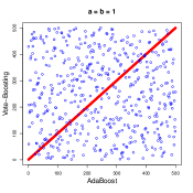
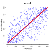
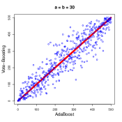
To investigate this relationship between vote-boosting and AdaBoost, we first present the results of an experiment in the binary classification problem Twonorm using decision stumps as base learners. In Twonorm, instances are drawn from two unit-variance Gaussians in $20$ dimensions whose means are $(a,a,\ldots,a)$ for class $1$ and $(-a,-a,\ldots,-a)$ for class $2$, with $a=2/\sqrt{20}$ [8]. This is not a trivial task for decision stumps because, as individual classifiers, they can model only class boundaries that are parallel to the axes. In the experiments performed, the training set is composed of $500$ independently generated instances. Different vote-boosting ensembles composed of $100$ stumps were built using the symmetric beta distribution for emphasis, with $a=b\in\left\{1.0,2.0,30.0\right\}$. An AdaBoost ensemble composed of $100$ stumps was also built using the same training data. The final weights given to the training instances in the different ensembles were recorded and subsequently ranked. Ties were resolved by randomizing the corresponding ranks. In Figure 2, a scatter plot of these ranks is shown where the ranks for AdaBoost are on the horizontal axis and in the vertical axis for vote-boosting with $a=b=1.0$ in (a), $a=b=2.0$ in (b), and $a=b=30.0$ in (c). When $a=b=1.0$ is used, all instances are assigned the same weight and no correlations between the weight ranks given by vote-boosting and AdaBoost can be observed. Therefore, the points corresponding to the training instances appear uniformly distributed in Figure 2 (a). As the values of $a=b$ increase, points tend to cluster around the diagonal. This is a consequence of the fact that the ranks of the weights given by both types of ensembles become more similar. Comparing Figs. 2 (a), (b) and (c), it is apparent that the correlations between the weight ranks become stronger as $a=b$ increases. In particular for $a=b=30.0$ vote-boosting and AdaBoost give similar emphasis, even though the former does not make use of class labels to decide whether an instance should be given more weight, whereas the latter does. The reason for this coincident emphasis is that, in this simple problem, the ensemble classifiers are more likely to disagree precisely in the instances that are incorrectly classified.

(a)

(b)

(c)

Figure 2: Weight ranks of the training instances for vote-boosting and AdaBoost of decision stumps in Twonorm (a) $a=b=1.0$, (b) $a=b=2.0$, (d) $a=b=30.0$

(a)

(b)

(c)

Figure 3: Weight ranks of the training instances for vote-boosting and AdaBoost of decision stumps in Twonorm with $30\%$ class-label noise, (a) $a=b=1.0$, (b) $a=b=2.0$, (c) $a=b=30.0$

If class-label noise is injected in the problem, the weighting schemes of AdaBoost and vote-boosting become different: Vote-boosting maintains the focus on instances in the boundary region, in which classes overlap and the disagreement rates among the ensemble predictions are highest. By contrast, AdaBoost tends to give more weight to those instances whose class label has been modified. Focusing on these noisy instances is misleading and eventually impairs the generalization capacity of AdaBoost. To illustrate this observation, the experiment was repeated injecting class-label noise in the training data. Specifically, 30% of the training examples were selected at random and their class labels flipped, as in the noisy completely at random model described in [18]. The results of these experiments are shown in Figure 3. Instances whose class label has been switched are marked with a red cross in these plots. For $a=b=1.0$, no correlation is observed between the ranks of the weights given by vote-boosting and AdaBoost. However, instances whose class label has been switched, which are distributed uniformly in the vertical direction, tend to appear on the right-hand side of the plots. This means that they receive special emphasis in AdaBoost but not in vote-boosting. Increasing the value of $a=b$ pushes the unperturbed instances towards the diagonal but not the perturbed ones. However, the correlation between the ranks is less prominent than in the noiseless case, because of the interference of the noisy instances.

(a)

(b)

Figure 4: Error rate as a function of number of classifiers in Twonorm for bagging, AdaBoost, and vote-boosting ensembles of pruned CART trees: (a) training error (b) test error.

(a)

(b)

Figure 5: Error rate as a function of the number of classifiers in Pima for bagging, AdaBoost, and vote-boosting ensembles of pruned CART trees: (a) training error (b) test error.

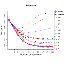
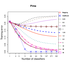
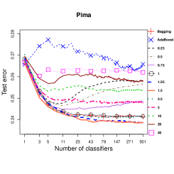
A second batch of experiments was carried out to analyze the behavior of vote-boosting composed of pruned CART trees as a function of the strength of the emphasis that is applied to uncertain instances. Using the symmetric beta distribution as emphasis function, we analyze how the learning curves, which trace the dependence of the error as a function of the size of the ensemble, depend on the value of the shape parameter. The values explored are $a$=$b\in\{0.25,0.5,0.75,1.0,1.25,1.5,2.5,5,10,20,40\}$. The experiments were made on the classification tasks Twonorm and Pima. These tasks have been chosen because of the different prediction accuracies of bagging and AdaBoost on those datasets. In Twonorm, AdaBoost significantly outperforms bagging. By contrast in Pima, which is a very noisy task, bagging is more accurate than AdaBoost.

Figure 4 and 5 display the learning curves for bagging, AdaBoost, and vote-boosting using different values of the shape parameter in the classification tasks Twonorm and Pima, respectively. The plots on the left-hand side show the results for the training error. The plots on the right-hand side correspond to the test error curves. When $a=b=1.0$, all instances are given equal weights. In this case, if weighted resampling is used, vote-boosting is equivalent to bagging. This is apparent from Figure 4 and 5: the error curves of both methods are very close to each other. When values $a=b<1.0$ are used, emphasis is made on instances on which most predictors agree. If regularized classifiers, such as pruned CART trees, are used as base learners, this type of emphasis is in general not effective. Nonetheless, as will be illustrated by the results presented in Section 4.3, focusing on these types of instances can lead to improvements in the generalization capacity when the data are very noisy and the ensemble is composed of flexible classifiers that overfit (e.g. unpruned CART or random trees).

Values of $a=b>1.0$ correspond to emphasizing instances in which the ensemble prediction is uncertain. For Twonorm, the learning curves of vote-boosting using $a=b=40.0$ and AdaBoost are quite similar. In this problem, the classification errors are mainly due to the overlap between the distributions of the two classes. Therefore, the incorrectly classified instances are close to the decision boundary, where the ensemble predictions are also more uncertain. Using a beta distribution sharply peaked around $\pi=0.5$ (see Figure 1) gives more weight to these uncertain instances. In consequence, the resulting emphasis is similar to AdaBoost’s. In Pima, which is a noisy problem, the learning curves of vote-boosting with large $a=b$ and AdaBoost are different. Still, the closest performance to AdaBoost is vote-boosting with large $a=b$. Finally, we observe that the optimal value for the shape parameter of the beta distribution in vote-boosting is problem dependent: Values of $a=b\approx 1.25-1.5$ perform well in Pima. The best performance in Twonorm requires using a large values of $a=b\approx 40$. For each problem, the optimal value can be determined using cross-validation.

4.2 Vote-boosting with different base learners

In this section, we present the results of a comparison of vote-boosting ensembles composed of different base learners. These are, in order of increasing complexity, decision stumps, pruned and unpruned CART trees, and unpruned random trees. Ensembles composed of $501$ classifiers are built. This fairly large ensemble size is needed in some problems to achieve convergence to the asymptotic error level [30]. Weighted resampling with replacement is used to generate the bootstrap samples on which the individual classifiers are trained. In vote-boosting, the symmetric beta distribution is used for emphasis. The shape parameter is determined as the value among those in $a$=$b\in$ {0.25, 0.5, 0.75, 1.0, 1.25, 1.5, 2.5, 5, 10, 20, 40} that minimizes the 10-fold cross-validation in the training set. When uniform emphasis in all the training instances ($a=b=1.0$) is used, the results are equivalent to bagging or, if random trees are used as base learners, to random forest. For values of the shape parameter above $1.0$, the symmetric beta distribution has a single mode at $\pi=0.5$, which implies that more emphasis is made on training instances on which the degree of disagreement among the different classifiers is large. By contrast, when the shape parameter is smaller than $1$ the focus is on training instances on which most classifiers agree.

For the empirical evaluation carried out in this an the following section, different binary classification tasks from the UCI repository [4] and other sources [9] are considered. The characteristics of the datasets used in this study are summarized in Table 1. For each dataset, the table displays the total number of labeled instances available, the number of those instances used for training and for testing, and the number of attributes. The test error rates reported are averages, followed by the corresponding standard deviations after the $\pm$ sign, over $100$ realizations of the training and test sets. For classification problems in which only a finite collection of labeled instances is available, $2/3$ of the data are selected at random for training and the remaining $1/3$ for testing. For synthetic problems (namely, Ringnorm, Twonorm, and Threenorm), instances are generated independently at random: $300$ instances are used for training and $2000$ for testing. In all cases, stratified sampling is used to ensure that the class distributions in the test and training sets are similar.

Table 1: Characteristics of the classification problems analyzed and training / test partitions.

Dataset	Instances	Training	Test	Number of
				attributes
Adult	32561	21707	10854	15
Australian	690	460	230	14
Breast W.	699	466	233	9
Blood	748	499	249	5
Boston	506	337	169	14
Chess	3196	2131	1065	36
German	1000	667	333	20
Heart	270	178	92	13
Hepatitis	155	104	51	19
Horse-colic	368	246	122	21
Ionosphere	351	234	117	34
Liver	345	230	115	6
Magic	19020	12680	6340	11
Musk	6598	4399	2199	168
Ozone	2536	1691	845	74
Parkinsons	197	132	65	24
Pima	768	512	256	8
Ringnorm	2300	300	2000	20
Sonar	208	139	69	60
Spambase	4601	3068	1533	58
Threenorm	2300	300	2000	20
Tic-tac-toe	958	639	319	9
Twonorm	2300	300	2000	20

In Table 2, the average test errors over the $100$ realizations are shown for all base learners. For each dataset, the lowest average generalization error is highlighted in boldface and the second best is underlined. If the differences between the two lowest test errors is statistically significant at a significance level $\alpha=0.05$ the lowest error value is marked with an asterisk (*). A resampled paired t-test is used for synthetic problems. When random train/test partitions of the same dataset are employed a corrected resampled paired t-test [42, 6] is used instead.

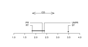
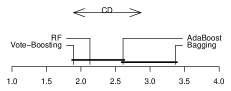
To provide an overall comparison of the accuracies of vote-boosting using the four tested base learners, we apply the framework proposed in [13]. To this end, the average rank of the classifier average errors is computed for the $23$ classification problems investigated. The rank of a classifier in a specific classification problem is determined by ordering the different methods according to their test errors. A lower rank corresponds to a smaller test error and, therefore, better accuracy. The average ranks of vote-boosting using the four different base learners are displayed in Figure 6. In this diagram, the differences of average ranks between methods that are connected by a horizontal solid line are not statistically significant according to a Nemenyi test (p-value $<$ 0.05).

From the results presented in Table 2 and Figure 6, one concludes that vote-boosting composed of random trees has the best overall accuracy: except in Boston, Horse-colic, and Parkinsons, these types of ensembles achieve the lowest or second lowest average test errors. Notwithstanding, according to the Nemenyi test, the average rank differences are statistically significant only with respect to the use of stumps (see Figure 6).

The values of the shape parameters of the symmetric beta distribution ($a=b$) selected by cross-validation are shown in Table 3. The figures reported are medians over the $100$ realizations of the training and test data. An asterisk is shown in the Table when ensembles built using the different values have the same within-train cross-validation error. For decision stumps, this occurs in Australian and Musk because the individual stumps are the same irrespective of the type of emphasis employed. In Musk, when more complex base classifiers are used, the ensembles built with the different values of $a=b$ all achieve zero error. In most cases, the value of the shape parameter of the beta distribution ($a=b$) decreases as the complexity of the base classifier increases. The reason of this is that more emphasis is needed in order to boost more stable base classifiers. Thus, the largest values of $a=b$ are selected for decision stumps. Hence, for these types of base learners the focus is on uncertain instances, on which most ensemble classifiers disagree. The lowest values of $a=b$ correspond to random trees. In this case, the emphasis on uncertain instances is reduced. In fact, for Blood, Heart, Musk, and Pima, the focus should be on instances on which the ensemble classifiers agree.

In summary, vote-boosting ensembles composed of random trees provide the best overall accuracy in the problems investigated. Since this type of ensemble can also be built efficiently, they will be used for further evaluation in the following set of experiments.

Table 2: Test error rates of vote-boosting ensembles composed of decision stumps, pruned CART trees, unpruned CART trees and random trees.

Dataset	Stump		Pruned		Unpruned		Random tree
Adult	20.9$\pm$	2.9	13.6$\pm$	0.3	13.5$\pm$	6.2	13.6$\pm$	0.2
Australian	14.6$\pm$	2.1	13.6$\pm$	2.0	13.5$\pm$	2.1	13.3$\pm$	2.1
Breast W.	3.9$\pm$	1.0	3.8$\pm$	1.1	4.0$\pm$	1.2	3.1$\pm$	1.1
Blood	22.7$\pm$	1.5	22.2$\pm$	1.7	21.8$\pm$	1.8	21.9$\pm$	1.7
Boston	15.2$\pm$	2.3	12.7$\pm$	2.5	13.0$\pm$	2.6	13.1$\pm$	2.3
Chess	17.7$\pm$	14.1	0.6$\pm$	0.6	0.7$\pm$	0.6	0.6$\pm$	0.3
German	25.4$\pm$	1.6	24.1$\pm$	2.1	24.1$\pm$	2.0	24.3$\pm$	1.7
Heart	16.4$\pm$	3.5	17.8$\pm$	3.6	18.4$\pm$	3.9	16.8$\pm$	3.5
Hepatitis	16.4$\pm$	4.3	16.2$\pm$	4.8	16.9$\pm$	4.9	14.0$\pm$	3.9
Horse-Colic	13.9$\pm$	2.7	14.1$\pm$	2.9	13.9$\pm$	2.7	15.0$\pm$	2.5
Ionosphere	8.1$\pm$	1.7	6.7$\pm$	2.0	6.7$\pm$	1.8	6.6$\pm$	1.8
Liver	27.5$\pm$	3.9	28.4$\pm$	3.6	28.6$\pm$	3.9	28.4$\pm$	3.7
Magic	15.4$\pm$	0.3	12.7$\pm$	0.3	12.9$\pm$	0.3	11.6$\pm$	0.2*
Musk	0.0$\pm$	0.0	0.0$\pm$	0.0	0.0$\pm$	0.0	0.0$\pm$	0.0
Ozone	6.3$\pm$	0.0	5.8$\pm$	0.4	5.8$\pm$	0.4	6.0$\pm$	0.2
Parkinsons	11.5$\pm$	4.3	7.4$\pm$	3.6	7.6$\pm$	3.2	9.3$\pm$	3.6
Pima	24.1$\pm$	2.0	24.2$\pm$	2.2	23.8$\pm$	2.3	23.4$\pm$	1.8
Ringnorm	9.3$\pm$	0.9	4.5$\pm$	0.8	4.6$\pm$	0.8	4.4$\pm$	0.8
Sonar	18.9$\pm$	4.6	16.0$\pm$	4.4	15.8$\pm$	4.8	15.5$\pm$	4.5
Spambase	6.1$\pm$	0.6	4.5$\pm$	0.3	4.5$\pm$	0.3	4.1$\pm$	0.5
Threenorm	20.1$\pm$	1.0	17.1$\pm$	1.1	17.0$\pm$	1.0	16.2$\pm$	1.0*
Tictactoe	22.0$\pm$	2.9	0.7$\pm$	0.6	0.7$\pm$	0.6	1.1$\pm$	0.7
Twonorm	4.6$\pm$	0.7	4.2$\pm$	0.6	4.2$\pm$	0.6	3.6$\pm$	0.5*

Table 3: Median of the beta distribution parameter ensembles composed of decision stumps, pruned CART trees, unpruned CART trees, and random trees. An asterisk is shown when all values of the beta parameter yield the same cross-validation error

Dataset	Stump	Pruned	Unpruned	Random tree
Adult	40.0	40.0	20.0	1.0
Australian	*	5.0	2.5	1.5
Breast W.	10.0	5.0	10.0	1.0
Blood	40.0	1.25	0.75	0.5
Boston	40.0	20.0	10.0	2.0
Chess	20.0	20.0	20.0	10.0
German	40.0	5.0	2.5	2.5
Heart	10.0	2.5	1.5	0.5
Hepatitis	10.0	10.0	5.0	2.5
Horse-Colic	20.0	1.5	1.5	1.5
Ionosphere	40.0	5.0	10.0	2.5
Liver	40.0	5.0	5.0	1.5
Magic	40.0	40.0	40.0	20.0
Musk	*	*	*	0.7
Ozone	40.0	10.0	5.0	1.5
Parkinsons	40.0	15.0	10.0	5.0
Pima	15.0	1.5	1.0	0.5
Ringnorm	40.0	20.0	20.0	20.0
Sonar	40.0	20.0	20.0	10.0
Spambase	40.0	20.0	20.0	20.0
Threenorm	40.0	10.0	10.0	5.0
Tictactoe	40.0	20.0	20.0	10.0
Twonorm	20.0	20.0	20.0	5.0

Figure 6: Comparison of the average ranks of decision stumps (ST), pruned CART trees (PR), unpruned CART trees (UNPR), and random trees (RT) using a Nemenyi test. Horizontal lines connect methods whose average ranks are not significantly different (p-value $<$ 0.05).

4.3 Comparison of vote-boosting with other ensemble methods

In this section, we carry out an comparison of vote-boosting ensembles and other related methods: bagging, AdaBoost and random forest. The classification problems considered and experimental protocol followed are the same as in the previous section. In each type of ensemble, the base classifier that performs best is used: pruned CART trees in AdaBoost, unpruned CART trees in bagging, and random trees in vote-boosting and random forest. Note that unpruned CART or random trees cannot be used in combination with AdaBoost because they generally achieve zero training error, which gives rise to singularities in the weight updates. As illustrated in the previous section, similar results are obtained with vote-boosting ensembles composed of unpruned or pruned CART trees. The adabag [3], ipred [43] and ranfomForest [33] packages in R have been used for AdaBoost, bagging, and random forest implementations, respectively. As in the previous subsection, ensembles of $501$ classifiers are used to guarantee convergence to the asymptotic error level. In both vote-boosting and AdaBoost, weighted resampling with replacement is used to take into account the different emphasis on the training instances. In AdaBoost, reweighting was considered as an alternative. However, as reported in the literature, similar or slightly better results are obtained when resampling instead of reweighting is used [15, 49].

The experiments are carried out on the original problem, and also with 10%, 20% and 30% class-label noise. Class-label noise is injected into the training set by randomly switching the class label of a random subset (10%, 20% and 30%) of the training instances. This type of label noise is know as completely at random noise (NCAR) [18]. An interesting observation is that, as the noise level increases, the values of the shape parameter that are selected tend to decrease.

Table 4: Test error rates for bagging (unpruned CART trees), boosting (pruned CART trees), random forest, and vote-boosting (random trees).

	Noise
Dataset	(in %)	Bagging		AdaBoost		Random forest		Vote-boosting		a=b (median)
Adult	0	14.6$\pm$	0.2	13.8$\pm$	0.2	13.6$\pm$	0.2	13.6$\pm$	0.2	1.0
	10	15.5$\pm$	0.3	14.3$\pm$	0.3	14.1$\pm$	0.3	14.0$\pm$	0.3	0.75
	20	17.0$\pm$	0.3	14.8$\pm$	0.2	14.8$\pm$	0.3	14.3$\pm$	0.2	0.25
	30	20.3$\pm$	0.3	15.1$\pm$	0.3	17.8$\pm$	0.3	15.1$\pm$	0.2	0.25
Australian	0	13.3$\pm$	2.1	13.7$\pm$	1.9	13.0$\pm$	2.0	13.3$\pm$	2.1	1.5
	10	14.9$\pm$	2.3	17.6$\pm$	2.4	13.6$\pm$	2.0	13.6$\pm$	2.1	0.75
	20	18.2$\pm$	2.9	24.3$\pm$	3.0	15.8$\pm$	2.2	14.3$\pm$	2.4*	0.25
	30	24.6$\pm$	3.8	32.0$\pm$	3.5	21.6$\pm$	3.0	18.2$\pm$	3.3*	0.25
Breast W.	0	4.6$\pm$	1.2	3.6$\pm$	1.0	3.0$\pm$	1.0	3.1$\pm$	1.1	1.0
	10	6.3$\pm$	1.6	6.9$\pm$	1.8	4.1$\pm$	1.2	3.5$\pm$	1.2*	0.5
	20	9.6$\pm$	2.5	12.0$\pm$	2.6	6.5$\pm$	1.9	4.1$\pm$	1.4*	0.25
	30	17.7$\pm$	3.0	20.9$\pm$	3.4	13.0$\pm$	2.7	6.8$\pm$	2.6*	0.25
Blood	0	26.3$\pm$	1.9	25.4$\pm$	2.1	24.5$\pm$	2.2	21.9$\pm$	1.7*	0.5
	10	28.5$\pm$	2.2	27.2$\pm$	2.5	26.6$\pm$	2.4	22.6$\pm$	2.0*	0.25
	20	31.6$\pm$	2.7	30.2$\pm$	2.6	29.7$\pm$	2.6	23.8$\pm$	2.5*	0.25
	30	35.8$\pm$	3.6	34.6$\pm$	3.8	34.2$\pm$	3.6	29.0$\pm$	4.5*	0.25
Boston	0	14.2$\pm$	2.4	12.7$\pm$	2.4	13.0$\pm$	2.4	13.1$\pm$	2.3	2.0
	10	16.2$\pm$	2.8	16.9$\pm$	2.5	14.5$\pm$	2.6	14.9$\pm$	2.5	0.5
	20	19.1$\pm$	3.3	22.2$\pm$	3.6	17.5$\pm$	3.2	16.2$\pm$	2.8	0.5
	30	26.4$\pm$	4.2	31.4$\pm$	4.0	24.6$\pm$	3.8	21.3$\pm$	4.4*	0.25
Chess	0	0.6$\pm$	0.3	0.5$\pm$	0.3	1.6$\pm$	0.4	0.6$\pm$	0.3	10.0
	10	5.1$\pm$	0.7	2.3$\pm$	0.5	2.1$\pm$	0.5	2.1$\pm$	0.5	1.25
	20	11.9$\pm$	1.2	3.6$\pm$	0.7	4.3$\pm$	0.9	4.0$\pm$	0.9	0.75
	30	22.4$\pm$	1.5	5.5$\pm$	0.9*	10.2$\pm$	1.3	7.9$\pm$	1.5	0.25
German	0	24.5$\pm$	2.0	24.8$\pm$	2.1	24.0$\pm$	1.8	24.3$\pm$	1.7	2.5
	10	26.2$\pm$	2.1	27.9$\pm$	2.1	25.3$\pm$	1.8	25.3$\pm$	1.9	1.0
	20	28.8$\pm$	2.4	32.2$\pm$	2.5	27.3$\pm$	2.2	27.4$\pm$	2.3	0.75
	30	32.3$\pm$	3.0	37.4$\pm$	2.8	31.0$\pm$	3.1	29.9$\pm$	3.2	0.5
Heart	0	19.5$\pm$	3.7	20.2$\pm$	3.4	17.2$\pm$	3.0	16.8$\pm$	3.5	0.5
	10	22.7$\pm$	4.2	24.9$\pm$	4.5	19.3$\pm$	3.7	18.7$\pm$	4.0	0.5
	20	26.0$\pm$	5.0	30.6$\pm$	5.1	22.7$\pm$	4.2	20.8$\pm$	4.0	0.375
	30	32.1$\pm$	5.4	36.3$\pm$	6.0	28.5$\pm$	5.8	25.8$\pm$	6.6	0.25
Hepatitis	0	15.8$\pm$	4.7	15.8$\pm$	4.0	13.6$\pm$	3.5	14.0$\pm$	3.9	2.5
	10	17.1$\pm$	4.7	20.0$\pm$	5.0	14.2$\pm$	3.9	15.3$\pm$	3.9	1.0
	20	21.0$\pm$	5.8	26.0$\pm$	6.9	17.6$\pm$	4.8	17.3$\pm$	4.5	0.5
	30	27.8$\pm$	7.8	33.6$\pm$	7.2	23.8$\pm$	7.3	21.9$\pm$	7.0	0.5
Horse-colic	0	14.9$\pm$	2.8	15.4$\pm$	2.6	15.0$\pm$	2.5	15.0$\pm$	2.5	1.5
	10	17.8$\pm$	3.5	21.2$\pm$	3.5	17.3$\pm$	2.9	17.4$\pm$	3.0	1.0
	20	23.4$\pm$	4.2	27.6$\pm$	4.7	21.3$\pm$	3.6	20.9$\pm$	3.7	0.625
	30	30.0$\pm$	5.6	34.9$\pm$	5.1	28.4$\pm$	4.6	28.2$\pm$	5.3	0.75

Table 5: Test error rates for bagging (unpruned CART trees), boosting (pruned CART trees), random forest, and vote-boosting (random trees).

	Noise
Dataset	(in %)	Bagging		AdaBoost		Random forest		Vote-boosting		a=b (median)
Ionosphere	0	8.0$\pm$	2.2	6.6$\pm$	1.8	6.6$\pm$	1.6	6.6$\pm$	1.8	2.5
	10	9.5$\pm$	2.7	10.5$\pm$	2.6	7.9$\pm$	2.2	7.9$\pm$	2.2	0.75
	20	13.1$\pm$	3.1	17.0$\pm$	3.5	10.9$\pm$	2.9	9.9$\pm$	3.1	0.5
	30	19.7$\pm$	4.5	26.4$\pm$	4.5	17.8$\pm$	4.6	15.7$\pm$	5.1	0.25
Liver	0	29.5$\pm$	3.9	30.5$\pm$	3.9	27.7$\pm$	3.8	28.4$\pm$	3.7	1.5
	10	31.7$\pm$	4.1	33.8$\pm$	4.5	31.0$\pm$	4.0	31.4$\pm$	3.8	1.0
	20	36.1$\pm$	4.3	37.8$\pm$	4.5	35.1$\pm$	4.4	35.7$\pm$	4.4	1.0
	30	39.9$\pm$	4.7	41.5$\pm$	4.7	39.6$\pm$	4.5	39.7$\pm$	4.9	0.875
Magic	0	12.3$\pm$	0.3	12.9$\pm$	0.3	12.0$\pm$	0.3	11.6$\pm$	0.2*	20.0
	10	12.9$\pm$	0.3	13.9$\pm$	0.3	12.4$\pm$	0.2	12.5$\pm$	0.2	1.25
	20	14.2$\pm$	0.4	14.4$\pm$	0.3	13.6$\pm$	0.4	13.3$\pm$	0.4*	0.5
	30	17.4$\pm$	0.5	15.0$\pm$	0.5	16.7$\pm$	0.4	14.6$\pm$	0.4*	0.25
Musk	0	0.0$\pm$	0.0	0.0$\pm$	0.0	0.0$\pm$	0.0	0.0$\pm$	0.0	0.7
	10	1.4$\pm$	0.3	0.6$\pm$	0.2	1.6$\pm$	0.3	0.1$\pm$	0.1*	0.25
	20	4.5$\pm$	0.4	0.9$\pm$	0.6	5.7$\pm$	0.4	0.8$\pm$	0.3	0.25
	30	12.0$\pm$	1.0	2.5$\pm$	1.2*	14.4$\pm$	1.2	5.1$\pm$	0.7	0.25
Ozone	0	6.0$\pm$	0.3	5.7$\pm$	0.4*	6.0$\pm$	0.2	6.0$\pm$	0.2	1.5
	10	6.2$\pm$	0.3	6.4$\pm$	0.5	6.0$\pm$	0.2	6.0$\pm$	0.3	5.0
	20	6.6$\pm$	0.6	9.7$\pm$	1.0	6.1$\pm$	0.4	6.2$\pm$	0.4	1.0
	30	9.1$\pm$	0.9	18.3$\pm$	1.5	7.9$\pm$	1.0	7.5$\pm$	1.2	0.5
Parkinsons	0	10.5$\pm$	4.0	7.1$\pm$	3.3*	10.2$\pm$	3.4	9.3$\pm$	3.6	5.0
	10	13.8$\pm$	4.2	12.9$\pm$	4.0	12.2$\pm$	3.7	12.7$\pm$	4.2	1.5
	20	18.6$\pm$	5.7	20.1$\pm$	5.9	16.2$\pm$	4.8	17.0$\pm$	4.9	0.75
	30	24.1$\pm$	5.5	28.0$\pm$	6.0	23.0$\pm$	5.8	22.6$\pm$	6.1	0.5
Pima	0	23.9$\pm$	1.9	25.9$\pm$	1.9	23.2$\pm$	2.0	23.4$\pm$	1.8	0.5
	10	25.9$\pm$	2.3	28.9$\pm$	2.3	24.7$\pm$	2.2	24.1$\pm$	2.4	0.25
	20	28.4$\pm$	2.6	32.9$\pm$	3.3	26.7$\pm$	2.5	25.3$\pm$	2.5*	0.25
	30	32.6$\pm$	3.0	38.4$\pm$	3.3	31.5$\pm$	2.8	29.8$\pm$	3.7*	0.5
Ringnorm	0	8.9$\pm$	1.8	4.3$\pm$	0.6*	6.0$\pm$	1.1	4.4$\pm$	0.8	20.0
	10	9.6$\pm$	1.7	7.6$\pm$	1.0	6.7$\pm$	1.2	6.1$\pm$	1.4*	10.0
	20	10.8$\pm$	1.8	13.0$\pm$	1.7	7.9$\pm$	1.4*	8.4$\pm$	1.8	1.25
	30	15.6$\pm$	2.9	22.2$\pm$	2.3	12.4$\pm$	2.4	12.5$\pm$	3.0	0.75
Sonar	0	22.4$\pm$	5.1	15.1$\pm$	4.6	17.9$\pm$	4.8	15.5$\pm$	4.5	10.0
	10	23.3$\pm$	5.5	20.7$\pm$	5.1	20.6$\pm$	5.4	19.7$\pm$	4.6	5.0
	20	26.9$\pm$	5.7	26.3$\pm$	5.3	24.2$\pm$	5.7	24.5$\pm$	5.6	1.25
	30	32.2$\pm$	5.0	34.6$\pm$	5.5	30.4$\pm$	5.4	30.4$\pm$	5.3	0.75
Spambase	0	5.9$\pm$	0.5	4.3$\pm$	0.4	5.0$\pm$	0.5	4.1$\pm$	0.5	20.0
	10	8.2$\pm$	0.8	6.1$\pm$	0.6	6.5$\pm$	0.6	6.3$\pm$	0.6	0.75
	20	11.5$\pm$	1.0	7.5$\pm$	0.7	9.4$\pm$	0.8	7.1$\pm$	0.7	0.25
	30	16.5$\pm$	1.1	10.3$\pm$	1.1	14.3$\pm$	1.0	8.6$\pm$	0.8*	0.25

Table 6: Test error rates for bagging (unpruned CART trees), boosting (pruned CART trees), random forest, and vote-boosting (random trees).

	Noise
Dataset	(in %)	Bagging		AdaBoost		Random forest		Vote-boosting		a=b (median)
Threenorm	0	19.0$\pm$	1.7	16.8$\pm$	0.8	16.6$\pm$	0.9	16.2$\pm$	1.0*	5.0
	10	20.6$\pm$	1.7	20.2$\pm$	1.2	18.5$\pm$	1.1	18.6$\pm$	1.2	1.5
	20	23.3$\pm$	1.8	24.9$\pm$	1.6	21.2$\pm$	1.3*	21.6$\pm$	1.5	1.25
	30	28.8$\pm$	2.1	32.0$\pm$	1.9	26.9$\pm$	2.0*	27.2$\pm$	2.5	0.62
Tic-tac-toe	0	2.1$\pm$	0.9	0.7$\pm$	0.6*	2.1$\pm$	1.0	1.1$\pm$	0.7	10.0
	10	5.7$\pm$	1.6	9.9$\pm$	1.8	5.9$\pm$	1.6	5.6$\pm$	1.6	2.5
	20	12.5$\pm$	2.2	20.6$\pm$	2.7	12.7$\pm$	2.6	13.0$\pm$	2.6	1.25
	30	23.5$\pm$	2.8	30.3$\pm$	2.9	22.2$\pm$	2.7	22.9$\pm$	2.9	0.75
Twonorm	0	6.4$\pm$	1.5	4.0$\pm$	0.5	3.9$\pm$	0.5	3.6$\pm$	0.5*	5.0
	10	7.3$\pm$	1.6	7.1$\pm$	0.9	4.8$\pm$	0.7*	4.9$\pm$	0.8	1.25
	20	9.3$\pm$	2.1	12.6$\pm$	1.6	6.6$\pm$	1.1	6.7$\pm$	1.2	0.75
	30	14.2$\pm$	2.3	21.5$\pm$	2.4	10.7$\pm$	1.7	9.6$\pm$	2.5*	0.5
win/draw/loss	0	12/11/0		6/13/4		9/14/0		—
	10	16/7/0		17/6/0		4/18/1		—
	20	18/5/0		16/7/0		7/14/2		—
	30	19/4/0		19/2/2		11/11/1		—

Figure 7: Comparison of the average ranks of bagging, AdaBoost, random forest and vote-boosting using a Nemenyi test. Horizontal lines connect methods whose average ranks are not significantly different (p-value $<$ 0.05). The plots correspond to datasets without injected noise (top left), with $10\%$ (top right), $20\%$ (bottom left), and $30\%$ class-label noise (bottom right).

The test error rates of the different ensembles and classification problems considered are displayed in Tables 4, 5, and 6. The results reported are averages, followed by the corresponding standard deviations after the $\pm$ sign, over $100$ realizations of the training and test set partitions. The median value for $a=b$ used in vote-boosting is reported in the last columns of Tables 4, 5, and 6. In these tables, the best and second best results for each classification problem are highlighted using bold face and underlined, respectively. In addition, the lowest test error rate is marked with an asterisk (*) if the improvement over to the second best is statistically significant, at a significance level $\alpha=0.05$. The significance of these differences is determined using a paired resampled t-test for synthetic problems, and to a corrected resampled paired t-test [42, 6] when random train/test partitions are used. Finally, the number of significant wins and losses when one compares the average accuracy of vote-boosting with each of the remaining ensembles, according to the aforementioned statistical test, are shown in the last row of Table 6. Draws correspond to differences of average accuracy that are not statistically significant.

From the results presented in these tables, it is clear that vote-boosting ensembles exhibit the best overall performance. In particular, it has the largest number of statistically significant wins at all noise levels. The tally is very favorable when one compares the average accuracy of vote-boosting with bagging: vote-boosting significantly outperforms bagging in $12$ out of the $23$ datasets (without injected noise). For 10%, 20% and 30% noise levels, the differences in number of wins become larger: vote-boosting significantly outperforms bagging in $16$, $18$ and $19$ out of the $23$ tested datasets, respectively. The comparison with AdaBoost on the explored datasets is also favorable to vote-boosting. In the original datasets (i.e.without injected noise) vote-boosting outperforms AdaBoost in $6$ out of $23$ datasets and is inferior in $4$ datasets: Ozone, Parkinsons, Ringnorm, and Tic-tac-toe). In this problems vote-boosting is second best; furthermore, its test error rates of vote-boosting are fairly close to AdaBoost. In these classification problems, except for Ozone, the shape parameter of the beta distribution used as emphasis function in vote-boosting is fairly high. This indicates a strong emphasis on uncertain examples, which has a similar effect as the emphasis on incorrectly classified instances that is characteristic of AdaBoost. On the other hand, in problems such as Blood, Heart, Liver or Pima, which are difficult for AdaBoost, vote-boosting selects low values for $a=b$, which implies that less emphasis is made on uncertain examples.

It is remarkable that, for some datasets, such as Blood, Heart, and Pima, and in most of the problems, for sufficiently high levels of class-label noise, values of $a=b$ below $1.0$ provide the best accuracy. In such cases, emphasis is made on instances on which the individual ensemble classifiers agree the most. The effectiveness of this type of emphasis, which is somewhat counter-intuitive, is a consequence of the large intrinsic variability of random trees. In fact, this effect is less prominent in ensembles of more stable base learners, such as decision stumps or pruned CART trees. As the noise level increases, the performance of AdaBoost rapidly deteriorates. By contrasnt vote-boosting is robust to class-label noise: it outperforms AdaBoost in $17$, $16$ and $19$ datasets for 10%, 20% and 30% injected noise, respectively.

Finally, vote-boosting is more accurate than random forest in $9$ out of the $23$ classification problems investigated for the noiseless case. In some cases, the improvements can be fairly large (e.g. Blood, Chess, Ringnorm, Sonar or Tic-tac-toe). In $14$ datasets the two methods have comparable accuracies. The accuracy improvements of random forests over vote-boosting are not statistically significant in any of the problems investigated. When the class labels are contaminated, vote-boosting performs significantly better in $4$, $7$ and $11$, and worse in $1$, $2$ and $1$ datasets for 10%, 20%, and 30% noise levels, respectively. Again, in the noisy datasets we see that, when random forest wins, the differences are typically small. By contrast, when vote-boosting wins, the differences are, in general, large.

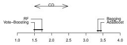
In addition, the overall performance of the accuracies of the different ensembles are summarized in Figure 7 using the procedure described in [13]. The plots in this figure display the average ranks of bagging, AdaBoost, random forest (RF) and vote-boosting for the original datasets (top left), and for 10% (top right), 20% (bottom left), 30% (bottom right) injected class-label noise. In these plots, a horizontal solid line connects methods for which the differences of average ranks are not statistically significant using a Nemenyi test with p-value $<$ 0.05. In the original problems, vote-boosting has the best average rank. However, the differences with random forest and AdaBoost are not statistically significant. The difference with bagging, which has the worst performance in terms average rank, is statistically significant. For problems contaminated with noise in the class labels, vote-boosting has the best average rank. The differences with respect to random forest increase for higher noise levels. However, they are not statistically significant. In all noisy problems, the average ranks of both random forest and vote-boosting ensembles are significantly better than bagging and AdaBoost.

Figure 8: Histograms of vote fractions for correctly (white) and incorrectly (red) classified instances in Sonar for the training set (left column) and test set (right column)

Figure 9: Histograms of vote fractions for correctly (white) and incorrectly (red) classified instances in Pima for the training set (left column) and test set (right column)

4.4 Emphasis profiles

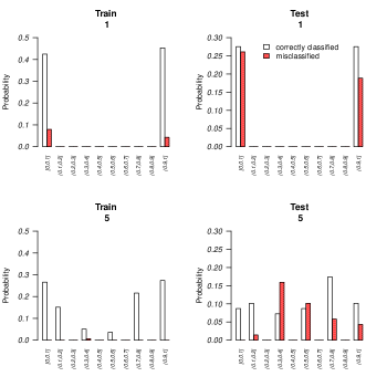
From the values of the shape parameter of the beta distribution reported in the last column of Tables 4, 5, and 6, it is apparent that the type of emphasis and its strength need to be adapted to the classification task considered. To further investigate this point, we have carried out a detailed analysis of the distribution of class votes for Sonar and Pima, in which the optimal emphasis strategies are very different.

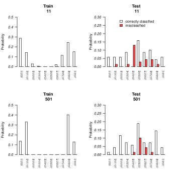
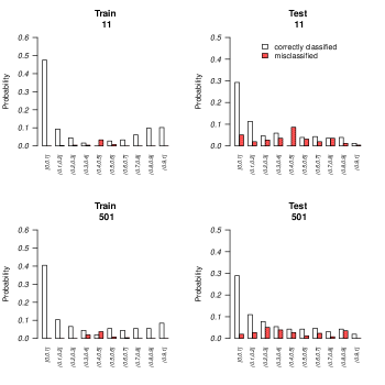
In Sonar, the vote-boosting ensemble is built using a beta distribution with $a=b=10.0$. Thus, the optimal emphasis is to focus on training instances in which the disagreement rates are largest. In Figure 8, the histograms of the distribution of votes are plotted for ensembles of $1$, $5$, $11$ and $501$ random trees. The height of the white bars indicate the fraction of correctly classified instances for the corresponding range of voting distributions. The red stripped bars correspond to incorrectly classified instances. The plots on the left are for the training set and on the right for the test set. In the training set, the strong focus on uncertain instances (those for which the fraction of class votes is close to $0.5$) leads to a markedly bimodal distribution, in which most predictions are by clear majority. Incorrectly classified instances disappear because ensembles that are sufficiently large achieve zero training error. The distribution of class votes in the test set is markedly different: It covers the whole interval, and exhibits a low peak for intermediate class vote frequencies, especially for instances that are misclassified.

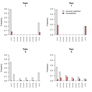
A very different picture is obtained in Pima (Figure 9). In this classification task, the selected shape parameter for the symmetric beta distribution is $a=b=0.5$. In consequence, the optimal strategy is to avoid focusing on training instances in which the disagreement rates are large. For correctly classified instances, the histograms in training and test sets are similar. Misclassified instances in the training set appear mostly around $0.5$. By contrast, in the test set, they appear in the whole $[0,1]$ interval. This is consistent with the observation that Pima has high levels of class-label noise.

5 Conclusions

Vote-boosting is a novel ensemble learning method in which individual classifiers are built using different weighted versions of the training data. To build a new classifier, the weights of the training instances are determined in terms of the disagreement rate among the classifiers that make up the ensemble at that point. The optimal weighing scheme depends on the complexity of the base classifiers and on the level of noise in the class labels of the training data. For simple or regularized classifiers, such as decision stumps or pruned CART trees, vote-boosting interpolates between bagging and AdaBoost. When the level of class-label noise is small, prediction errors are more likely to occur near the classification boundary, where the uncertainty, as measured by the disagreement among ensemble predictions, is largest. Therefore, it is possible to build more accurate ensembles by focusing on uncertain instances. Since these instances are more likely to be misclassified, the emphasis given by vote-boosting is similar to AdaBoost’s. For noisy classification problems, a softer emphasis on uncertain instances is generally preferable. In this case, the most accurate predictions are obtained by means of ensembles that are fairly similar to bagging. When more brittle individual learners are used (e.g. unpruned CART or random trees) a milder emphasis on uncertain instances is generally needed to achieve the best generalization performance. This is a consequence of the fact that some of the uncertainty in the predictions is due to the intrinsic variability of the base learners. For problems in which the level of class-label noise is high it is in fact advantageous to progressively focus on instances in which the ensemble classifiers agree. In practice, the optimal type of emphasis can be readily determined using cross-validation within the training data.

Note that, since AdaBoost is based on emphasizing incorrectly classified instances, it cannot be used to improve the performance of base learners whose training error is small, such as unpruned CART or random trees. By contrast, vote-boosting does not have this limitation and can be used to build boosted ensembles composed of these types of classifiers that are both accurate and robust to noise in the class labels.

References

- Abe et al. [2006] Abe, N., Zadrozny, B., Langford, J., 2006. Outlier detection by active learning. In: KDD ’06: Proceedings of the 12th ACM SIGKDD international conference on Knowledge discovery and data mining. ACM Press, New York, NY, USA, pp. 767–772.
- Ahachad et al. [2015] Ahachad, A., Omari, A., Figueiras-Vidal, A. R., 2015. Neighborhood guided smoothed emphasis for real adaboost ensembles. Neural Processing Letters 42 (1), 155–165.
- Alfaro et al. [2013] Alfaro, E., Gámez, M., García, N., 2013. adabag: An R package for classification with boosting and bagging. Journal of Statistical Software 54 (2), 1–35.
-
Bache and Lichman [2013]
Bache, K., Lichman, M., 2013. UCI machine learning repository.
URL http://archive.ics.uci.edu/ml - Bauer and Kohavi [1999] Bauer, E., Kohavi, R., july 1999. An Empirical Comparison of Voting Classification Algorithms: Bagging, Boosting, and Variants. Machine Learning 36 (1), 105–139.
- Bouckaert and Frank [2004] Bouckaert, R. R., Frank, E., 2004. Evaluating the Replicability of Significance Tests for Comparing Learning Algorithms. Springer Berlin Heidelberg, Berlin, Heidelberg, pp. 3–12.
Breiman [1996a]
Breiman, L., Aug 1996a. Bagging predictors. Machine Learning
24 (2), 123–140.
URL https://doi.org/10.1023/A:1018054314350 - Breiman [1996b] Breiman, L., 1996b. Bias, variance, and arcing classifiers. Tech. Rep. 460, Statistics Department, University of California.
- Breiman [1998] Breiman, L., 1998. Arcing classifiers. Annals of Statistics 26, 801–823.
Breiman [2000]
Breiman, L., Sep 2000. Randomizing outputs to increase prediction accuracy.
Machine Learning 40 (3), 229–242.
URL https://doi.org/10.1023/A:1007682208299 - Breiman [2001] Breiman, L., 2001. Random forests. Machine Learning 45 (1), 5–32.
- Cheamanunkul et al. [2014] Cheamanunkul, S., Ettinger, E., Freund, Y., 2014. Non-convex boosting overcomes random label noise. Computing Research Repository abs/1409.2905.
Demšar [2006]
Demšar, J., 2006. Statistical comparisons of classifiers over multiple
data sets. Journal of Machine Learning Research 7, 1–30.
URL http://www.jmlr.org/papers/volume7/demsar06a/demsar06a.pdf - Dietterich [2000a] Dietterich, T. G., 2000a. Ensemble Methods in Machine Learning. Lecture Notes in Computer Science 1857, 1–15.
- Dietterich [2000b] Dietterich, T. G., 2000b. An experimental comparison of three methods for constructing ensembles of decision trees: Bagging, boosting, and randomization. Machine Learning 40 (2), 139–157.
- Domingo and Watanabe [2000] Domingo, C., Watanabe, O., 2000. MadaBoost: A modification of AdaBoost. In: Proceedings of the Thirteenth Annual Conference on Computational Learning Theory. COLT ’00. pp. 180–189.
- Fernández-Delgado et al. [2014] Fernández-Delgado, M., Cernadas, E., Barro, S., Amorim, D., 2014. Do we need hundreds of classifiers to solve real world classification problems? Journal of Machine Learning Research 15, 3133–3181.
- Frénay and Verleysen [2014] Frénay, B., Verleysen, M., 2014. Classification in the presence of label noise: A survey. IEEE Transactions on Neural Networks and Learning Systems 25 (5), 845–869.
- Freund [2001] Freund, Y., 2001. An adaptive version of the boost by majority algorithm. Machine Learning 43 (3), 293–318.
Freund [2009]
Freund, Y., 2009. A more robust boosting algorithm.
URL http://arxiv.org/abs/0905.2138v1 - Freund et al. [1999] Freund, Y., Schapire, R., Abe, N., 1999. A short introduction to boosting. Journal-Japanese Society For Artificial Intelligence 14 (771-780), 1612.
- Freund and Schapire [1997] Freund, Y., Schapire, R. E., 1997. A decision-theoretic generalization of on-line learning and an application to boosting. Journal of Computer and System Sciences 55 (1), 119 – 139.
- Friedman et al. [2000] Friedman, J., Hastie, T., Tibshirani, R., Apr. 2000. Additive logistic regression: a statistical view of boosting (With discussion and a rejoinder by the authors). The Annals of Statistics 28 (2), 337–407.
- Fumera and Roli [2005] Fumera, G., Roli, F., June 2005. A theoretical and experimental analysis of linear combiners for multiple classifier systems. IEEE Transactions on Pattern Analysis and Machine Intelligence 27 (6), 942–956.
- Geurts et al. [2006] Geurts, P., Ernst, D., Wehenkel, L., 2006. Extremely randomized trees. Machine Learning 63 (1), 3–42.
- Gómez-Verdejo et al. [2008] Gómez-Verdejo, V., Arenas-García, J., Figueiras-Vidal, A. R., 2008. A dynamically adjusted mixed emphasis method for building boosting ensembles. IEEE Transactions on Neural Networks 19 (1), 3–17.
- Gómez-Verdejo et al. [2006] Gómez-Verdejo, V., Ortega-Moral, M., Arenas-García, J., Figueiras-Vidal, A. R., 2006. Boosting by weighting critical and erroneous samples. Neurocomputing 69 (7-9), 679–685.
- Guo et al. [2002] Guo, Y., Bartlett, P. L., Smola, A. J., Williamson, R. C., Baxter, J., 2002. Norm-based regularization of boosting. Technical ReportAustralian National University.
- Hansen and Salamon [1990] Hansen, L. K., Salamon, P., Oct 1990. Neural network ensembles. IEEE Transactions on Pattern Analysis and Machine Intelligence 12 (10), 993–1001.
- Hernández-Lobato et al. [2011] Hernández-Lobato, D., Martínez-Muñoz, G., Suárez, A., 2011. Inference on the prediction of ensembles of infinite size. Pattern Recognition 44 (7), 1426 – 1434.
- Jiang [2001] Jiang, W., 2001. Is regularization unnecessary for boosting? In: Department of Statistics, Northwestern University. Morgan Kaufmann, pp. 57–64.
- Khoshgoftaar et al. [2011] Khoshgoftaar, T. M., Hulse, J. V., Napolitano, A., May 2011. Comparing boosting and bagging techniques with noisy and imbalanced data. IEEE Transactions on Systems, Man, and Cybernetics - Part A: Systems and Humans 41 (3), 552–568.
- Liaw and Wiener [2002] Liaw, A., Wiener, M., 2002. Classification and regression by randomforest. R News 2 (3), 18–22.
- Liu and Yao [1999] Liu, Y., Yao, X., 1999. Ensemble learning via negative correlation. Neural Networks 12, 1399–1404.
- Long and Servedio [2010] Long, P. M., Servedio, R. A., 2010. Random classification noise defeats all convex potential boosters. Machine Learning 78 (3), 287–304.
- Loureiro et al. [2004] Loureiro, A., Torgo, L., Soares, C., 2004. Outlier detection using clustering methods: a data cleaning application. In: Proceedings of KDNet Symposium on Knowledge-based Systems for the Public Sector. Bonn, Germany.
- Maclin and Opitz [2011] Maclin, R., Opitz, D. W., 2011. Popular ensemble methods: An empirical study. Computing Research Repository abs/1106.0257.
- Martínez-Muñoz and Suárez [2005] Martínez-Muñoz, G., Suárez, A., 2005. Switching class labels to generate classification ensembles. Pattern Recognition 38 (10), 1483–1494.
- Mason et al. [2000] Mason, L., Baxter, J., Bartlett, P., Frean, M., 2000. Boosting algorithms as gradient descent. In: Advances in Neural Information Processing Systems 12. MIT Press, pp. 512–518.
- Mayhua-Lopez et al. [2012] Mayhua-Lopez, E., Gomez-Verdejo, V., Figueiras-Vidal, A. R., Dec 2012. Real adaboost with gate controlled fusion. IEEE Transactions on Neural Networks and Learning Systems 23 (12), 2003–2009.
- McDonald et al. [2003] McDonald, R. A., Hand, D. J., Eckley, I. A., 2003. An empirical comparison of three boosting algorithms on real data sets with artificial class noise. In: Multiple Classifier Systems, 4th International Workshop, MCS 2003, Guilford, UK, June 11-13, 2003, Proceedings. pp. 35–44.
Nadeau and Bengio [2003]
Nadeau, C., Bengio, Y., Sep 2003. Inference for the generalization error.
Machine Learning 52 (3), 239–281.
URL https://doi.org/10.1023/A:1024068626366 - Peters and Hothorn [2009] Peters, A., Hothorn, T., 2009. ipred: improved predictors. R package version 0.8-8.
- Quinlan [1996] Quinlan, J. R., 1996. Bagging, Boosting, and C4.5. In: Proceedings of the Thirteenth National Conference on Artificial Intelligence. pp. 725–730.
- Rätsch et al. [1998] Rätsch, G., Onoda, T., Müller, K. R., 1998. An improvement of adaboost to avoid overfitting. In: Proceedings of the International Conference on Neural Information Processing. Citeseer.
- Rodríguez et al. [2006] Rodríguez, J. J., Kuncheva, L. I., Alonso, C. J., 2006. Rotation forest: A new classifier ensemble method. IEEE Transactions on Pattern Analysis Machine Intelligence 28 (10), 1619–1630.
- Schapire [1990] Schapire, R. E., 1990. The strength of weak learnability. Machine Learning 5, 197–227.
- Schapire and Freund [2012] Schapire, R. E., Freund, Y., 2012. Boosting: Foundations and Algorithms. The MIT Press.
- Seiffert et al. [2008] Seiffert, C., Khoshgoftaar, T. M., Hulse, J. V., Napolitano, A., Nov. 2008. Resampling or Reweighting: A Comparison of Boosting Implementations. In: 20th International Conference on Tools with Artificial Intelligence. pp. 445–451.
- Shivaswamy and Jebara [2011] Shivaswamy, P. K., Jebara, T., 2011. Variance penalizing adaboost. In: Shawe-Taylor, J., Zemel, R. S., Bartlett, P. L., Pereira, F. C. N., Weinberger, K. Q. (Eds.), NIPS. pp. 1908–1916.
- Sun et al. [2004] Sun, Y., Li, J., Hager, W. W., 2004. Two new regularized adaboost algorithms. In: Proceedings of the 2004 International Conference on Machine Learning and Applications - ICMLA 2004, 16-18 December 2004, Louisville, KY, USA. pp. 41–48.
- Sun et al. [2006] Sun, Y., Todorovic, S., Li, J., 2006. Reducing the overfitting of adaboost by controlling its data distribution skewness. International Journal of Pattern Recognition and Artificial Intelligence 20 (7), 1093–1116.
- Tulyakov et al. [2008] Tulyakov, S., Jaeger, S., Govindaraju, V., Doermann, D., 2008. Machine Learning in Document Analysis and Recognition. Springer Berlin Heidelberg, Ch. Review of Classifier Combination Methods.