Curved branes with regular support

Abstract

We study spacetime singularities in a general five-dimensional braneworld with curved branes satisfying four-dimensional maximal symmetry. The bulk is supported by an analog of perfect fluid with the time replaced by the extra coordinate. We show that contrary to the existence of finite distance singularities from the brane location in any solution with flat (Minkowski) branes, in the case of curved branes there are singularity-free solutions for a range of equations of state compatible with the null energy condition.

1 Introduction

In previous work we studied the singularity structure of a braneworld model consisting of a flat $3$-brane embedded in a five-dimensional bulk space filled with an analogue of a perfect fluid (the fifth coordinate $Y$ playing the role of time). The perfect fluid satisfied a linear equation of state with a constant parameter $\gamma$, $P=\gamma\rho$, where $P$ is the ‘pressure’ and $\rho$ is the ‘density’. In [1] we showed that for a flat brane there exist singularities that appear within finite distance $Y_{0}$ from the position of the brane supposedly located at the origin, for all values of $\gamma$. A way to avoid such singularities is to exploit the natural $Z_{2}$ symmetry introduced by the existence of the brane by cutting the bulk space and considering a slice of it which is free from finite-distance singularities. Although this matching mechanism is possible for all values of $\gamma$, the requirement for localised gravity on the brane restricts $\gamma$ in the interval $(-2,-1)$. On the other hand, further requirements for physical conditions, such as energy conditions, restrict $\gamma$ in values greater than $-1$. Therefore within the framework of our flat brane model it is not possible to satisfy at the same time the positive energy conditions and the condition for localised gravity on the brane.

A question that naturally arises is whether any of the above conclusions about the existence of singularities are sensitive to the geometry of the brane so that singularities are absent when we consider a curved brane. It was proposed in [2], [3] that the singularity present in the flat brane model moves to infinite distance when the brane becomes curved, such as de Sitter (dS) or anti-de Sitter (AdS) in the maximally symmetric case, which was in accordance with previous claims made in [4].

In this paper, we show that this is indeed possible. In particular, we show that for curved branes there exist ranges of $\gamma$ for which finite-distance singularities are avoided; these are: $\gamma>-1/2$ (for positively curved brane) and $-1<\gamma<-1/2$ (for negatively curved brane). For each type of brane geometry and values of $\gamma$ outside these regions, we find that finite-distance singularities continue to exist. A way to be removed is by using the cutting and matching procedure mentioned above to construct a slice of non-singular bulk space, when that is possible. Moreover, imposing the null energy condition (guaranteeing the absence of ghosts in the bulk) excludes de Sitter (dS) branes and one is left only with the second region of $\gamma$ for Anti-de Sitter (AdS) branes. However, we further show that this region in AdS branes is incompatible with having also localised gravity on the brane. The situation is not improved when allowed non-singular solutions obtained by the cutting and matching procedure.

The plan of this paper is the following: In Sections $2$ and $3$, we present the model and give the exact solutions respecting 4d maximal symmetry, as well as the complete list of all asymptotic behaviours for all ranges of the parameters in our model. In Section $4$, we analyse in detail the two non-singular solutions found in Section $3$. In Section $5$, we derive the null energy condition and investigate its consequences. In Section $6$ we construct non-singular orbifold-like solutions, called matching in the following, obtained by the cutting and matching procedure for those cases that allow it, and study the null energy condition. In Section $7$, we examine whether the previously derived solutions also satisfy the condition for localisation of gravity on the brane. Section $8$ contains a summary of our results and some concluding remarks. Finally, in Appendix A we derive the solutions found for two special values of the parameter $\gamma$ that cannot be incorporated in the solutions given in Section $3$.

2 The setup for a curved brane model

Our braneworld model consists of a 3-brane embedded in a five-dimensional bulk space $\mathcal{M}\times\mathbb{R}$ filled with an analogue of a perfect fluid with equation of state $P=\gamma\rho$, where the ‘pressure’ $P$ and the ‘density’ $\rho$ are functions only of the fifth dimension, $Y$. The bulk metric is of the form

$$g_{5}=a^{2}(Y)g_{4}+dY^{2},$$ (2.1)

where $g_{4}$ is the four-dimensional de Sitter or anti de Sitter metric, i.e.,

$$g_{4}=-dt^{2}+f^{2}_{k}g_{3},$$ (2.2)

with

$$g_{3}=dr^{2}+h^{2}_{k}g_{2},$$ (2.3)

and

$$g_{2}=d\theta^{2}+\sin^{2}\theta d\varphi^{2},$$ (2.4)

where $f_{k}=\cosh(Ht)/H$ or $\cos(Ht)/H$ ($H^{-1}$ is the de Sitter (or AdS) curvature radius) and $h_{k}=\sin r$ or $\sinh r$, respectively.

The metric (2.1) is a warped product on $\mathbb{R}\times_{a}\mathcal{M}$ the warping factor being positive $a(Y)>0$, it may be considered as a generalization of the standard Riemannian cone metric $dS^{2}=dY^{2}+Y^{2}g_{4}$ on $\mathbb{R}\times_{a}\mathcal{M}$ [5], [6]. The bulk fluid has an energy-momentum tensor of the form

$$T_{AB}=(\rho+P)u_{A}u_{B}-Pg_{AB},$$ (2.5)

where $A,B=1,2,3,4,5$ and $u_{A}=(0,0,0,0,1)$, with the 5th coordinate corresponding to $Y$. The five-dimensional Einstein equations,

$$G_{AB}=\kappa^{2}_{5}T_{AB},$$ (2.6)

can be written in the following form:

$$\frac{a^{\prime\prime}}{a} = -2A\frac{(1+2\gamma)}{3}\rho,$$ (2.7)

$$\frac{a^{\prime 2}}{a^{2}} = \frac{2A}{3}\rho+\frac{kH^{2}}{a^{2}},$$ (2.8)

where $A=\kappa_{5}^{2}/4$, $k=\pm 1$, and the prime $(\,^{\prime})$ denotes differentiation with respect to $Y$. The equation of conservation,

$$\nabla_{B}T^{AB}=0,$$ (2.9)

becomes

$$\rho^{\prime}+4(1+\gamma)\frac{a^{\prime}}{a}\rho=0.$$ (2.10)

Integration of the continuity equation (2.10) gives the following relation between the density and the warp factor,

$$\rho=c_{1}a^{-4(\gamma+1)},$$ (2.11)

where $c_{1}$ is an arbitrary integration constant. Substitution of Eq. (2.11) in Eq. (2.8), gives

$$a^{\prime 2}=\dfrac{2}{3}Ac_{1}a^{-2(2\gamma+1)}+kH^{2},$$ (2.12)

and after setting $C=2/3Ac_{1}$ (note the the sign of $C$ is the same with the sign of $\rho$), we have the Friedman constraint in the form,

$$a^{\prime 2}=Ca^{-2(2\gamma+1)}+kH^{2}.$$ (2.13)

The left hand side of this equation restricts the signs of $C$ and $k$, as well as the range of $a$. As a result, the case $C<0$ and $k<0$ becomes automatically impossible.

On the other hand, the case $C<0$, $k>0$ is possible only for,

$$\textrm{dS braneworld:}\quad 0<a^{-2(2\gamma+1)}<-\dfrac{kH^{2}}{C},$$ (2.14)

while, the case $C>0$, $k<0$ is possible only for

$$\textrm{AdS braneworld:}\quad a^{-2(2\gamma+1)}>-\dfrac{kH^{2}}{C}>0.$$ (2.15)

It is straightforward to see that these two cases offer the possibility for avoidance of singularities. More generally, our solutions below are characterised by these three constants, namely, the curvature constant $k$, the fluid constant $\gamma$, and the constant $C$, where as mentioned above the sign of $C$ controls that of the density $\rho$.

The case $C<0$, $k>0$ of a dS brane with $\gamma>-1/2$, implies that $a^{2(2\gamma+1)}>-C/(kH^{2})>0$, so that the warp factor, $a$, is bounded away from zero, excluding therefore collapse singularities from happening. The only way that this case may introduce a finite-distance singularity is to have a warp factor that becomes divergent within a finite distance (big-rip singularity). However, it will follow from our analysis in the next Section that this behaviour is also excluded and therefore this case does indeed lead to the avoidance of finite-distance singularities. On the other hand, the case $C>0$, $k<0$ of an AdS brane with $\gamma<-1/2$, implies that the warp factor takes only values greater than $-kH^{2}/C>0$, thus excluding the existence of collapse singularities, as well. As we will show later on, this latter case requires a further restriction on $\gamma$, $-1<\gamma<-1/2$, in order to avoid a finite-distance big-rip singularity.

3 Analysis of the Friedman equation

Eq. (2.13) can be integrated out to give a solution represented by the Gaussian hypergeometric function ${}_{2}F_{1}$, for all possible cases defined by the signs of $C$ and $k$ and the range of $\gamma$ . These solutions along with the asymptotic behaviours they introduce are presented in what follows. The values $\gamma=-1$ and $\gamma=-1/2$ are special values for our system of equations (2.7), (2.8) and (2.10) in the sense that they reduce it to a significantly simpler form which leads to solutions that cannot be incorporated into the solutions found below with the use of the Gaussian hypergeometric function. The solutions for these values of $\gamma$ are studied separately in Appendix A, however, in order to have a complete view of the asymptotics for all possible values of $\gamma$ immediately, we present the behaviors of the solutions for $\gamma=1,-1/2$ in the Subsections 3.1, 3.2 and 3.3 that follow.

3.1 dS branes with positive density

We begin our study with the case of a dS braneworld with positive density. This corresponds to $C>0$, $k>0$, and depending on the range of $\gamma$ we have the following sub-cases:

• For $\gamma<-1/2$, the solution is,

  $$\pm(Y-Y_{0})=\dfrac{a}{\sqrt{kH^{2}}}\,_{2}F_{1}\left(\dfrac{1}{2},-\dfrac{1}{2(2\gamma+1)},\dfrac{4\gamma+1}{2(2\gamma+1)},-\dfrac{C}{kH^{2}}a^{-2(2\gamma+1)}\right).$$ (3.1)

• For $\gamma>-1/2$, we have,

  $$\pm(Y-Y_{0})=\dfrac{1}{2(\gamma+1)\sqrt{C}}a^{2(\gamma+1)}\,_{2}F_{1}\left(\dfrac{1}{2},\dfrac{\gamma+1}{2\gamma+1},\dfrac{3\gamma+2}{2\gamma+1},-\dfrac{kH^{2}}{C}a^{2(2\gamma+1)}\right).$$ (3.2)

The possible asymptotic behaviours follow from those of the hypergeometric function ${}_{2}F_{1}$:

1. $\gamma\geq-1/2$ we find that $a\rightarrow 0$, as $Y\rightarrow Y_{0}$. This is a collapse type singularity and it appears within a finite distance, at $Y_{0}$.

2. $\gamma\geq-1/2$ we have that $a\rightarrow\infty$, as $Y\rightarrow\infty$, which describes the behaviour of the warp factor at infinite distance.

3. $\gamma\leq-1/2$ the behaviour here is $a\rightarrow 0$, as $Y\rightarrow Y_{0}$, so that we have a collapse singularity at $Y_{0}$.

4. $-1\leq\gamma\leq-1/2$ we get $a\rightarrow\infty$, as $Y\rightarrow\infty$, which is as before the behaviour of the warp factor at infinite distance.

5. $\gamma<-1$, in this case $a\rightarrow\infty$, as $Y\rightarrow Y_{0}\pm\delta$, where the constant $\delta$ is given by:

   $$\delta=\dfrac{\Gamma((1+4\gamma)(2(2\gamma+1))\Gamma((\gamma+1)/(2\gamma+1))}{\sqrt{\pi}(kH^{2})^{\frac{\gamma+1}{2\gamma+1}}}C^{\frac{1}{2(2\gamma+1)}}$$ (3.3)

   where $\Gamma$ is the Gamma function. This is a big rip singularity and it appears within finite distance, at $Y_{0}\pm\delta$.

For $\gamma<-1$ there are two types of finite-distance singularities: a collapse singularity located at $Y_{0}$, and a big-rip singularity located at $Y_{0}\pm\delta$. As we will show later, the coexistence of these two types of singularity not only does not lead to non-singular spacetimes, but it also impedes the construction of any non-singular matching solution for $\gamma<-1$.

On the other hand, for $\gamma\geq-1$, the braneworld suffers only from a finite-distance singularity of the collapse type, which allows for the construction of a matching non-singular solution.

3.2 dS branes with negative density

We now consider a dS braneworld with negative density, corresponding to $C<0$, $k>0$, and let $\gamma$ varying as follows:

• $\gamma<-1/2$, the solution is given by (3.1).

• $\gamma>-1/2$, the solution is,

  $$\pm(Y-Y_{0}) = \dfrac{(-C)^{-\frac{\gamma}{2\gamma+1}}(kH^{2})^{\frac{-1}{2(2\gamma+1)}}}{2(2\gamma+1)}\sqrt{a^{2(2\gamma+1)}+\dfrac{C}{kH^{2}}}\times$$ (3.4)

  $$\times_{2}F_{1}\left(\dfrac{1}{2},\dfrac{\gamma}{2\gamma+1},\dfrac{3}{2},1+\dfrac{kH^{2}}{C}a^{2(2\gamma+1)}\right).$$

The solutions in this case satisfy the bounds (2.14) and we arrive at the following asymptotic behaviours:

1. $\gamma\leq-1/2$ here $a\rightarrow 0$ as $Y\rightarrow Y_{0}$, and this is a collapse singularity appearing at $Y_{0}$. There is no other singularity since $a$ is bounded from above and never diverges.

2. $\gamma>-1/2$ we see that $a\rightarrow\infty$ as $Y\rightarrow\infty$, which means that this case is free from finite-distance singularities, since $a$ is bounded from below and never vanishes.

3.3 AdS branes with positive density

The last possible case is that of an open universe with positive density support on the bulk which translates to considering $C>0$ and $k<0$ (AdS braneworld). Taking into account the possible ranges of $\gamma$ we have the following outcomes:

• $\gamma>-1/2$ or, $\gamma<-1$ the solution is given by Eq. (3.2).

• $-1<\gamma<-1/2$ the solution is,

  $$\pm(Y-Y_{0}) = -\dfrac{C^{\frac{\gamma+1}{2\gamma+1}}}{2(2\gamma+1)(-kH^{2})^{\frac{4\gamma+3}{4\gamma+2}}}\sqrt{a^{-2(2\gamma+1)}+\dfrac{kH^{2}}{C}}\,\times$$ (3.5)

  $$\times {}_{2}F_{1}\left(\dfrac{4\gamma+3}{2(2\gamma+1)},\dfrac{1}{2},\dfrac{3}{2},1+\dfrac{C}{kH^{2}}a^{-2(2\gamma+1)}\right).$$

As we mentioned earlier, this case is subject to the bound (2.15) The possible asymptotic behaviours for this case are then as follows:

1. $\gamma\geq-1/2$ we find $a\rightarrow 0$, as $Y\rightarrow Y_{0}$, which implies a collapse singularity at $Y_{0}$; the warp factor is bounded from above.

2. $-1\leq\gamma<-1/2$ we find $a\rightarrow\infty$ as $Y\rightarrow\infty$, so that this region of $\gamma$ is free form finite distance singularities, since $a$ is again bounded from below and never vanishes.

3. $\gamma<-1$ we have $a\rightarrow\infty$, as $Y\rightarrow Y_{0}$. This is a big-rip singularity located at $Y_{0}$. There is no collapse singularity since $a$ is bounded from below.

4 Non-singular solutions

We saw in the previous Section that there are solutions free from finite-distance singularities in the following cases:

• dS brane with negative density and $\gamma>-1/2$

• AdS brane with positive density and $-1\leq\gamma<-1/2$.

In this Section we analyse the complete character of these two non-singular solutions.

The first non-singular solution is given by Eq. (3.4) for $\gamma>-1/2$. The two branches of this solution may be matched in the following way. Let $\hat{Y}$ denote the value of $Y$ for which $a^{-2(2\gamma+1)}$ is equal to $-kH^{2}/C$, that is

$$(a(\hat{Y}))^{-2(2\gamma+1)}=-\dfrac{kH^{2}}{C}.$$ (4.1)

Then we see from Eq. (3.4) that the value of the Gaussian hypergeometric function at $\hat{Y}$ is equal to one, while from the left-hand side of the same equation we find that $\hat{Y}=Y_{0}$. We note that $Y_{0}$ is a regular point of the solution. Putting Eq. (4.1) in Eq. (2.13) we find that

$$a^{\prime}(Y_{0})=0,$$ (4.2)

so that $Y_{0}$ is a critical point. We now check the second derivative of $a$, $a^{\prime\prime}$. For $C<0$ it follows from Eq. (2.11) and the fact that $c_{1}=3C/(2A)$ that also $\rho<0$. Further assuming $\gamma>-1/2$, we find from Eq (2.7) that

$$a^{\prime\prime}(Y_{0})>0.$$ (4.3)

Thus, for this choice of parameters we see that at $Y_{0}$ the warp factor takes its minimum value and then it starts to increase, avoiding in this way collapse singularities.

To study the behaviour of the solution at infinity i.e. as $a\rightarrow\infty$, we expand the hypergeometric function as follows [7],

$${}_{2}F_{1}\left(\dfrac{1}{2},\dfrac{\gamma}{2\gamma+1},\dfrac{3}{2},1+\dfrac{kH^{2}}{C}a^{2(2\gamma+1)}\right)=\Gamma_{1}\left(-1-\dfrac{kH^{2}}{C}a^{2(2\gamma+1)}\right)^{-1/2}\times$$ (4.4)

$$\times {}_{2}F_{1}\left(\frac{1}{2},0,\frac{4\gamma+3}{2(2\gamma+1)},\left(1+\frac{kH^{2}}{C}a^{2(2\gamma+1)}\right)^{-1}\right)+\Gamma_{2}\left(-1-\frac{kH^{2}}{C}a^{2(2\gamma+1)}\right)^{-\frac{\gamma}{2\gamma+1}}\times$$

$$\times {}_{2}F_{1}\left(\frac{\gamma}{2\gamma+1},-\frac{1}{2(2\gamma+1)},\frac{4\gamma+1}{2(2\gamma+1)},\left({1+\frac{kH^{2}}{C}a^{2(2\gamma+1)}}\right)^{-1}\right),$$

where

$$\Gamma_{1}=\frac{\sqrt{\pi}\,\Gamma(-1/(2(2\gamma+1)))}{2\Gamma(\gamma/(2\gamma+1))}$$ (4.5)

and

$$\Gamma_{2}=\frac{\Gamma(1/(2(2\gamma+1)))}{2\Gamma((4\gamma+3)/(2(2\gamma+1)))}.$$ (4.6)

Substituting in the solution (3.4) we find,

$$\pm(Y-Y_{0})\sim a,$$ (4.7)

and so we see from (4.7) that $a\rightarrow\infty$ is only possible for $Y\rightarrow\pm\infty$. The behaviour of $a$ is shown in Fig. 1.

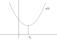
Figure 1: Non-singular solution for $C<0$, $k>0$ and $\gamma>-1/2$, or $C>0$, $k<0$ and $-1<\gamma<-1/2$.

For an AdS braneworld on the other hand, the solution (3.5) is non-singular for $-1<\gamma<-1/2$. We note that because of Eq. (2.15), the warp factor $a$ for this range of $\gamma$ cannot approach zero and therefore all collapse singularities are excluded from happening, however, the possibility of the warp factor becoming divergent within finite distance is not a priori prohibited. If such behaviour is encountered then we end up with an even stronger type of singularity, a big rip.

Let us suppose that the warp factor does become divergent, $a\rightarrow\infty$, but restrict $\gamma$ in the interval $(-1,-1/2)$. The hypergeometric function appearing in Eq. (3.5) has the argument $1+Ca^{-2(2\gamma+1)}/(kH^{2})$ which is diverging so to study its behaviour at infinity, we first expand it in the following way,

$${}_{2}F_{1}\left(\dfrac{4\gamma+3}{2(2\gamma+1)},\dfrac{1}{2},\dfrac{3}{2},1+\dfrac{C}{kH^{2}}a^{-2(2\gamma+1)}\right)=$$

$$\Gamma_{3}\left(-1-\dfrac{C}{kH^{2}}a^{-2(2\gamma+1)}\right)^{-\frac{(4\gamma+3)}{4\gamma+2}}\times$$

$$\times_{2}F_{1}\left(\dfrac{4\gamma+3}{2(2\gamma+1)},\dfrac{\gamma+1}{2\gamma+1},\dfrac{3\gamma+2}{2\gamma+1},\left(1+\dfrac{C}{kH^{2}}a^{-2(2\gamma+1)}\right)^{-1}\right)+$$

$$+\Gamma_{4}\left(-1-\dfrac{C}{kH^{2}}a^{-2(2\gamma+1)}\right)^{-1/2}\,_{2}F_{1}\left(\dfrac{1}{2},0,\dfrac{\gamma}{2\gamma+1},\left(1+\dfrac{C}{kH^{2}}a^{-2(2\gamma+1)}\right)^{-1}\right),$$ (4.8)

where $\Gamma_{3}$ and $\Gamma_{4}$ are the constants,

$$\Gamma_{3}=\dfrac{\Gamma(-(\gamma+1)/(2\gamma+1))}{2\Gamma(\gamma/(2\gamma+1))},$$ (4.9)

and

$$\Gamma_{4}=\dfrac{\sqrt{\pi}\,\Gamma((\gamma+1)/(2\gamma+1))}{2\Gamma((4\gamma+3)/(2(2\gamma+1)))}.$$ (4.10)

Substituting the above expression of the hypergeometric function in the solution (3.5), we deduce the asymptotic behaviour,

$$\pm(Y-Y_{0})\sim a^{2(\gamma+1)},$$ (4.11)

so that for $a\rightarrow\infty$, we get $Y\rightarrow\pm\infty$. Therefore the divergence of the warp factor is only possible at infinite distance which means that finite-distance big rip singularities are excluded. The behaviour of $a$ is similar to the one shown in Fig. 1.

5 The null energy condition

In this Section we study the null energy condition for our type of matter (2.5) and then examine for which ranges of $\gamma$ it holds true.

We note that our metric (2.1) and our fluid are static with respect to the time coordinate $t$. We may reinterpret our fluid analogue as a real anisotropic fluid having the following energy momentum tensor:

$$T_{AB}=(\rho^{0}+p^{0})u_{A}^{0}u_{B}^{0}+p^{0}g_{\alpha\beta}\delta_{A}^{\alpha}\delta_{B}^{\beta}+p_{Y}g_{55}\delta_{A}^{5}\delta_{B}^{5},$$ (5.1)

where $u_{A}^{0}=(a(Y),0,0,0,0)$, $A,B=1,2,3,4,5$ and $\alpha,\beta=1,2,3,4$. When we combine (2.5) with (5.1), we get the following set of relations,

$$p_{Y} = \rho$$ (5.2)

$$\rho^{0} = p$$ (5.3)

$$p^{0} = -p.$$ (5.4)

The last two relations imply that

$$p^{0}=-\rho^{0},$$ (5.5)

which means that this type of matter satisfies a cosmological constant-like equation of state. Imposing further $p=\gamma\rho$, and using (5.2), leads to,

$$p_{Y}=\frac{p}{\gamma}.$$ (5.6)

Substituting (5.4), (5.5) and (5.6) in (5.1), we find that

$$T_{AB}=-pg_{\alpha\beta}\delta_{A}^{\alpha}\delta_{B}^{\beta}+\frac{p}{\gamma}g_{55}\delta_{A}^{5}\delta_{B}^{5}.$$ (5.7)

We are now ready to form the null energy condition for our type of matter. According to the null energy condition, every future-directed null vector $k^{A}$ should satisfy [8]

$$T_{AB}k^{A}k^{B}\geq 0.$$ (5.8)

This condition implies that the energy density should be non-negative. Here we find that it translates to

$$p+\dfrac{p}{\gamma}\geq 0,$$ (5.9)

or, in terms of $\rho$

$$(\gamma+1)\rho\geq 0,$$ (5.10)

which leads to two possible cases, namely,

$$\rho\geq 0\quad\textrm{and}\quad\gamma\geq-1,\quad\textrm{or,}\quad\rho\leq 0\quad\textrm{and}\quad\gamma\leq-1.$$ (5.11)

With the use of (2.11), in which $c_{1}=3/(2A)C$, these two conditions may be written equivalently with respect to $C$ instead of $\rho$ as,

$$C\geq 0\quad\textrm{and}\quad\gamma\geq-1,$$ (5.12)

and

$$C\leq 0\quad\textrm{and}\quad\gamma\leq-1.$$ (5.13)

The conditions (5.12) and (5.13) show that the requirement of satisfying the null energy condition leads to restrictions on both the range of $\gamma$ and the sign of the constant $C$. We conclude that the only range for $C$ and $\gamma$ that is compatible with a non-singular solution, and at the same time also satisfies the null energy condition, is $C>0$ and $-1<\gamma<-1/2$ combined with $k<0$, that is AdS braneworld with positive density and $\gamma\in(-1,-1/2)$. In particular, dS non-singular braneworlds are incompatible with the null energy condition holding in the bulk.

6 Matching solutions

In this Section we will examine those solutions from the Sections 3.1-3.3, that allow a jump in the derivative of the warp factor, $a^{\prime}$, across the brane, and also satisfy the null energy condition. These are the cases $Ia)$ and $Ib)$.

For the case $Ia)$, we have $\gamma<-1/2$, and for the null energy condition we should further restrict to $-1<\gamma<-1/2$. Setting $c_{2}=\mp Y_{0}$, and choosing the $+$ sign of $Y$ for $Y>0$ and the $-$ sign for $Y<0$, the solution (3.1) can be written in the form

$$|Y|+c_{2}^{\pm}=\dfrac{a}{\sqrt{kH^{2}}}\,_{2}F_{1}\left(\dfrac{1}{2},-\dfrac{1}{2(2\gamma+1)},\dfrac{4\gamma+1}{2(2\gamma+1)},-\dfrac{C}{kH^{2}}a^{-2(2\gamma+1)}\right).$$ (6.1)

For $c_{2}^{\pm}>0$, we see that collapse singularities are excluded. Since we have restricted $\gamma$ to take values greater than $-1$, big-rip singularities are also excluded. Assuming a continuous warp factor at the position of the brane $Y=0$, we get from (6.1) a condition for $c_{2}$ which reads,

$$c_{2}^{+}=c_{2}^{-},$$ (6.2)

where $c_{2}^{\pm}$ denote the values of $c_{2}$ at $Y=0^{\pm}$. Note that $c_{2}^{\pm}$ are both positive from (6.1) which is compatible with our choice of sign for $c_{2}$. Further imposing continuity of $\rho$ at $Y=0$, we find from (2.11) and $c_{1}=3/(2A)C$ that

$$C^{+}=C^{-}.$$ (6.3)

Next, we take into account the jump of the derivative of the warp factor across the brane. For our type of geometry this junction condition reads

$$a^{\prime}(0^{+})-a^{\prime}(0^{-})=-\dfrac{1}{3}f(\rho(0))a(0),$$ (6.4)

where $f(\rho)$ is the tension of the brane. For our solution the above condition translates to

$$f(\rho(0))=-6\sqrt{kH^{2}a^{-2}(0)+Ca^{-4(\gamma+1)}(0)},$$ (6.5)

from which we note that the brane tension is negative.

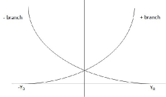
Figure 2: Non-singular matching solution for $C>0$, $k>0$ and $-1<\gamma<-1/2$. We take the $(+)$ branch for $Y>0$ and the $(-)$ branch for $Y<0$.

In Fig. $2$, we depict the two branches of the solution and the way they may be matched together to give the non-singular solution described above.

Similarly, we may match the two branches of solution of case $Ib)$ for $\gamma>-1/2$, and find,

$$|Y|+c_{2}^{\pm}=\dfrac{1}{2(\gamma+1)\sqrt{C}}a^{2(\gamma+1)}\,_{2}F_{1}\left(\dfrac{1}{2},\dfrac{\gamma+1}{2\gamma+1},\dfrac{3\gamma+2}{2\gamma+1},-\dfrac{kH^{2}}{C}a^{2(2\gamma+1)}\right).$$ (6.6)

It follows that conditions (6.2)-(6.5) are also true in this case. The two branches of the solution and the way they may be matched together to give the non-singular solution are shown in Fig. $3$.

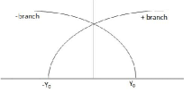
Figure 3: Non-singular matching solution for $C>0$, $k>0$ and $\gamma>-1/2$. We take the $(+)$ branch for $Y>0$ and the $(-)$ branch for $Y<0$.

We can also have a matching solution by cutting the regular solutions $IIb)$, or, $IIIb)$ at a point different from the minimum (cutting the regular solutions at the minimum would lead to a vanishing brane tension). For example by taking $Y_{0}\neq 0$ and putting the brane at $Y=0$ we can derive the corresponding junction conditions which are again given by (6.2)-(6.4). The brane tension, however, now reads

$$f(\rho(0))=-12\sqrt{kH^{2}a^{-2}(0)+Ca^{-4(\gamma+1)}(0)},$$ (6.7)

and we note that it is again negative.

The rest of the cases $II$ and $III$ that satisfy the null energy condition for $\gamma<-1$ ($IIa$) and $\gamma>-1$ ($IIIa$), respectively, are not suitable for constructing non-singular matching solutions since they exhibit either two collapse (case $IIIa$), or two big rip singularities (case $IIIa)$) that restrict $Y$ to take values only between the interval with endpoints the two finite singularities. That means that the resulting matching solutions cannot be extended to the whole real line of $Y$.

7 Localisation of gravity

Another question we would like to answer is whether the non-singular solutions we have found for the warp factor $a$, satisfying the null energy condition, lead to a finite four-dimensional Planck mass, thus localising 4d gravity on the brane for some range of the parameter $\gamma$. The value of the four-dimensional Planck mass, $M_{p}^{2}=8\pi/\kappa$, is determined by the following integral [9],

$$\frac{\kappa_{5}^{2}}{\kappa}=\int_{-Y_{c}}^{Y_{c}}a^{2}(Y)dY.$$ (7.1)

For our first matching solution, Eq. (6.1), the behaviour of $a^{2}$ at large $|Y|$ is

$$a^{2}\sim(|Y|+c_{2})^{2},$$ (7.2)

and the above integral becomes,

$$\int_{-Y_{c}}^{Y_{c}}(|Y|+c_{2})^{2}dY=\dfrac{1}{3}\left(-(-Y+c_{2})^{3}|_{-Y_{c}}^{0}+(Y+c_{2})^{3}|_{0}^{Y_{c}}\right).$$ (7.3)

In the limit $Y_{c}\rightarrow\infty$, the Planck mass becomes infinite.

The same behavior is valid also for the regular solution $IIb)$ found for a dS brane with negative density and $\gamma>-1/2$. Placing the brane at $Y=0$ and using the line of thinking of Section $6$ we can bring the left hand side of solution (3.4) into a form involving the absolute value of $Y$. Then Eq. (4.7) can take the form of (7.2) which lead to an infinite Planck mass.

For our second matching solution (6.6), the behaviour of $a^{2}$ is

$$a^{2}\sim(|Y|+c_{2})^{\frac{1}{\gamma+1}}.$$ (7.4)

Integration of $a^{2}$ gives an expression with $Y$ raised to the exponent,

$$\dfrac{\gamma+2}{\gamma+1}$$ (7.5)

which is positive for this case since here $\gamma>-1/2$. Therefore we see that the Planck mass is infinite also in this case.

As before the same behavior is valid for the other regular solution $IIIb)$ of an AdS brane with positive density and $-1<\gamma<-1/2$. For this solution we could also place the brane at $Y=0$ and by using its asymptotic behavior given by Eq. (4.11) we see that it could take the form of (7.4) and therefore lead to an infinite Planck mass since $\gamma$ does not lie in $(-2,-1)$.

8 Conclusions

In this paper, we have analysed braneworld singularities in the presence of dS or AdS branes and found one non-singular solution for a dS brane with negative (bulk) density and another one for an AdS brane with positive (bulk) density, for particular ranges of the parameter space, that we constructed explicitly. As we showed in [1] this was impossible for Minkowski branes. In the case of AdS branes the null energy condition is also satisfied.

Comparing and contrasting the results of the asymptotic behaviour of the solutions found in this paper to those of our previous work [3] which was implemented with a different method of asymptotic analysis we extract the following conclusions: The case of a dS brane with positive density, described in Section 3.1, was asymptotically constructed by the two balances simultaneously ${}_{\gamma}\mathcal{B}_{1}$ and ${}_{\gamma}\mathcal{B}_{2}$. The first balance described the behavior of $a$ around a finite collapse singularity, while the second balance described the behavior of $a$ at infinity. In particular, the balance ${}_{\gamma}\mathcal{B}_{2}$ gave the behavior, $a\rightarrow\infty$ as $Y\rightarrow\infty$, however, this case is characterised as singular because of the finite-distance singularity of collapse type introduced by the balance ${}_{\gamma}\mathcal{B}_{1}$.

On the other hand, the case of an AdS brane with positive density, described in Section 3.2, was depicted by the balance ${}_{\gamma}\mathcal{B}_{2}$ which is non-singular for $\gamma>-1/2$. The balance ${}_{\gamma}\mathcal{B}_{1}$ which leads to finite-distance singularities for flat and positively curved branes is not valid in this case since it assumes only positive density, whereas, this case is characterised by a negative density. Lastly, the third case, described in Section 3.3, can be described by the balance ${}_{\gamma}\mathcal{B}_{1}$ which allows for a non-singular solution for $-1<\gamma<-1/2$.

It is possible that non-singular solutions that satisfy the null energy condition in the bulk and at the same time localize gravity in the braneworld exist for models of interacting matter as in [10], or, for homogeneous but anisotropic (eg. Bianchi I, V, or VIII, IX) braneworlds. Exploring such models will help us decide about the stability of our non-singular solutions discovered here with respect to more general (anisotropic) perturbation. We leave this to a future publication.

Appendix A Appendix: Solutions for curved branes and special fluids

In this Appendix we analyze the behavior of the system of equations (2.7)-(2.8) and (2.10) for special values of the parameter $\gamma$ of the fluid. These are values of $\gamma$ that simplify the dynamical system significantly and lead to solutions that cannot be incorporated to the solutions found in Section $3$. These special values are $\gamma=-1/2$ and $\gamma=-1$.

Consider first $\gamma=-1/2$. Eqs. (2.7)-(2.8) and (2.10) for $\gamma=-1/2$ become

$$a^{\prime\prime} = 0$$ (A.1)

$$\dfrac{{a^{\prime}}^{2}}{a^{2}} = \dfrac{\kappa_{5}^{2}}{6}\rho+\dfrac{kH^{2}}{a^{2}}$$ (A.2)

$$\rho^{\prime}+2\dfrac{a^{\prime}}{a}\rho = 0.$$ (A.3)

Eq. (A.1) gives directly

$$a=c_{1}Y+c_{2},$$ (A.4)

where $c_{1}$ and $c_{2}$ are arbitrary constants. Inputting (A.4) in Eq. (A.3) we find

$$\rho=\dfrac{{c}_{3}}{(c_{1}Y+c_{2})^{2}},$$ (A.5)

where $c_{3}$ is an arbitrary constant. We substitute Eqs. (A.4) and (A.5) in Eq. (A.2) to derive the relation between the three arbitrary constants which reads

$$c_{3}=\dfrac{6}{\kappa_{5}^{2}}({c_{1}}^{2}-kH^{2}).$$ (A.6)

The linear solution (A.4) shows that for $\gamma=-1/2$, $a\rightarrow 0$ at a finite-distance

$$Y_{0}=-\dfrac{c_{2}}{c_{1}},$$ (A.7)

and also $a\rightarrow\infty$ as $Y\rightarrow\infty$. This case therefore suffers from a finite-distance collapse singularity.

For $\gamma=-1$, on the other hand, the dynamical system given by Eqs. (2.7)-(2.8) and (2.10) takes the form

$$\dfrac{a^{\prime\prime}}{a} = \dfrac{\kappa_{5}^{2}}{6}\rho$$ (A.8)

$$\dfrac{{a^{\prime}}^{2}}{a^{2}} = \dfrac{\kappa_{5}^{2}}{6}\rho+\dfrac{kH^{2}}{a^{2}}$$ (A.9)

$$\rho^{\prime} = 0.$$ (A.10)

Eq. (A.10) implies that

$$\rho=c_{3},$$ (A.11)

with $c_{3}$ an arbitrary constant. By substitution of this in Eq. (A.8) we get the following second order differential equation with constant coefficients

$$a^{\prime\prime}-\kappa_{5}^{2}\dfrac{c_{3}}{6}a=0$$ (A.12)

which has the characteristic equation

$$\lambda^{2}-\kappa_{5}^{2}\dfrac{c_{3}}{6}=0.$$ (A.13)

For $c_{3}>0$ the above equation has two distinct real roots

$$\lambda=\pm\kappa_{5}\sqrt{\dfrac{c_{3}}{6}}$$ (A.14)

and so the general solution has the form

$$a=c_{1}e^{{\kappa_{5}}\sqrt{c_{3}/6}Y}+c_{2}e^{{-\kappa_{5}}\sqrt{c_{3}/6}Y},\quad c_{3}>0,$$ (A.15)

where $c_{1}$ and $c_{2}$ are arbitrary constants. Substituting (A.15) in Eq. (A.9) we find the relation connecting the three arbitrary constants which reads

$$c_{3}=-\dfrac{3kH^{2}}{2c_{1}c_{2}\kappa_{5}^{2}}.$$ (A.16)

Since we have taken $c_{3}>0$ we need to have the following restrictions on the signs of $c_{1}$, $c_{2}$ and $k$

$$\textrm{either}\quad c_{1}c_{2}<0\quad\textrm{and}\quad k>0,\quad\textrm{or,}\quad c_{1}c_{2}>0\quad\textrm{and}\quad k<0.$$ (A.17)

For $c_{1}c_{2}<0$ there is a finite-distance singularity at

$$Y_{0}=\dfrac{\sqrt{6}}{2\kappa_{5}\sqrt{c_{3}}}\ln\left(-\dfrac{c_{2}}{c_{1}}\right).$$ (A.18)

We also see from the solution (A.15) that $a$ becomes infinite only at infinite $Y$. For $c_{1}c_{2}>0$ and $k<0$, however, we see that the solution is free from finite-distance singularities.

For $c_{3}<0$, on the other hand, we have a different behavior. Taking $c_{3}<0$ translates first from Eq. (A.11) to having negative density and then from Eq. (A.9) to allowing only for a dS brane. For $c_{3}<0$ the characteristic equation has imaginary roots and the general solution (A.15) becomes complex. However, we can still obtain a real general solution from the complex one by imposing real initial conditions. The real general solution obtained in this way is given by

$$a=c_{1}\cos\left(\kappa_{5}\sqrt{\dfrac{C_{3}}{6}}Y\right)+c_{2}\sin\left(\kappa_{5}\sqrt{\dfrac{C_{3}}{6}}Y\right),$$ (A.19)

where $C_{3}=-c_{3}>0$. This solution has an infinite number of finite-distance singularities.

References

- [1] I. Antoniadis, S. Cotsakis, I. Klaoudatou, Enveloping branes and braneworld singularities, Eur. Phys. J. C74 (2014) 3192, [arXiv:hep-th/1406.0611v2].
- [2] I. Antoniadis, S. Cotsakis, I. Klaoudatou, Braneworld cosmological singularities, Proceedings of MG11 meeting on General Relativity, vol. 3, pp. 2054-2056, [arXiv:gr-qc/0701033].
- [3] I. Antoniadis, S. Cotsakis, I. Klaoudatou, Brane singularities and their avoidance, Class. Quant. Grav. 27 (2010) 235018 [arXiv:gr-qc/1010.6175].
- [4] S. S. Gubser, Curvature singularities: The good, the bad, and the naked, Adv. Theor. Math. Phys. 4 (2000) 679, [arXiv:hep-th/0002160].
- [5] P. Peterson, Riemannian geometry, Springer 2006.
- [6] B. O’ Neill, Semi-Riemannian geometry with applications to relativity, Academic Press 1983.
- [7] Z. X. Wang, D. R. Guo, Special Functions, World Scientific, 1989.
- [8] E. Poisson, A Relativist’s Toolkit, Cambridge University Press, 2004.
- [9] S. Forste, H. P. Nilles and I. Zavala, Nontrival Cosmological Constant in Brane Worlds with Unorthodox Lagrangians, JCAP 1107 (2011) 007, [arXiv:hep-th/1104.2570].
- [10] Antoniadis, I., Cotsakis, S. and Klaoudatou, I., Brane singularities with mixtures in the bulk, Fortschr. Phys. 61 (2013) 20-49.