Variations of the Interstellar Extinction Law within the Nearest Kiloparsec

Pulkovo Astronomical Observatory, Russian Academy of Sciences, Pulkovskoe sh. 65, St. Petersburg, 196140 Russia

Key words: interstellar dust grains, Galactic solar neighborhood, color–color diagrams, main sequence: early-type (O and B) stars, giants and subgiants.

Multicolor photometry from the Tycho-2 and 2MASS catalogues for 11 990 OB and 30 671 K-type red giant branch stars is used to detect systematic large-scale variations of the interstellar extinction law within the nearest kiloparsec. The characteristic of the extinction law, the total-to-selective extinction ratio $R_{V}$, which also characterizes the size and other properties of interstellar dust grains, has been calculated for various regions of space by the extinction law extrapolation method. The results for the two classes of stars agree: the standard deviation of the “red giants minus OB” $R_{V}$ differences within 500 pc of the Sun is 0.2. The detected $R_{V}$ variations between 2.2 and 4.4 not only manifest themselves in individual clouds but also span the entire space near the Sun, following Galactic structures. In the Local Bubble within about 100 pc of the Sun, $R_{V}$ has a minimum. In the inner part of the Gould Belt and at high Galactic latitudes, at a distance of about 150 pc from the Sun, $R_{V}$ reaches a maximum and then decreases to its minimum in the outer part of the Belt and other directions at a distance of about 500 pc from the Sun, returning to its mean values far from the Sun. The detected maximum of $R_{V}$ at high Galactic latitudes is important when allowance is made for the interstellar extinction toward extragalactic objects. In addition, a monotonic increase in $R_{V}$ by 0.3 per kpc toward the Galactic center has been found near the Galactic equator. It is consistent with the result obtained by Zasowski et al. (2009) for much of the Galaxy. Ignoring the $R_{V}$ variations and traditionally using a single value for the entire space must lead to systematic errors in the calculated distances reaching 10%.

THE METHOD

The interstellar extinction law describes the dependence of extinction $A_{\lambda}$ on emission wavelength $\lambda$. Since the extinction is difficult to measure directly at various wavelengths, the reddening of a star, i.e., the deviation of its color from the true one due to selective extinction, is traditionally measured to determine the extinction law. In the visual spectral range, the reddening $E_{(B-V)}$ is commonly considered. The reddening is currently believed to be produced by dust grains whose size is smaller than the emission wavelength. In the visual spectral range, these grains are less than 1 micron in size.

The extinction, for example, in the $V$ band is determined by taking into account the reddening: $A_{V}=R_{V}\cdot E_{(B-V)}$. The coefficient $R_{V}$ is the total-to-selective extinction ratio. The same (nonselective or “gray”) extinction at all wavelengths is apparently produced by dust grains with a size larger than the wavelength, i.e., more than 1 microns, for the visual spectral range. Therefore, $R_{V}$ and similar coefficients for other wavelengths (for example, $A_{Ks}/E_{(H-Ks)}$), first, reflect the fraction of coarse dust in the absorbing matter and the mean dust grain size and, second, possibly other dust grain properties. Since these coefficients, the wavelength, and the grain size are related between themselves, any of these coefficients is apparently a single versatile characteristic of the extinction law in a particular region of space and time (Fitzpatrick and Massa 2007). Given that the extinction law is often determined at present not for the visual range but for the infrared in the form of a coefficient similar to $R_{V}$, below we use the more general name “extinction law” instead of the “coefficient $R_{V}$”.

The reddening of a star is traditionally measured as the difference of the observed color and the zero point – the color of an unreddened star of the same spectral type. As was shown in the review by Perryman (2009), the natural scatter of colors for unreddened stars of the same spectral subtype (even if we forget the common classification errors) is typically $0.3^{m}$. Because of such a low accuracy, this method becomes a thing of the past in the cases where the individual reddenings or extinctions are averaged for a group of stars.

Using Present-Day Surveys

The new, basically statistical method based on the all-sky photometric surveys of millions of stars that have appeared in recent years gives a much smaller error. These surveys include the Tycho-2 catalogue (Høg et al. 2000) containing photometry in the $B_{T}$ and $V_{T}$ bands with the effective wavelengths $\lambda_{B_{T}}=0.435$ and $\lambda_{V_{T}}=0.505$ microns (for comparison, Johnson s $V$ band has $\lambda_{V}=0.553$ microns), the 2MASS catalogue (Skrutskie et al. 2006) with infrared photometry in the $J$ ($\lambda_{J}=1.24$ microns), $H$ ($\lambda_{H}=1.66$ microns), $Ks$ ($\lambda_{Ks}=2.16$ microns) bands (for comparison, Johnson s $K$ band has $\lambda_{V}=2.22$ microns), and other surveys. Owing to accurate photometry, the stars from such surveys are grouped by classes on color–color and color–magnitude diagrams. This allows the stars of certain classes to be selected and the mean characteristics of the selected stars in sky fields or spatial cells can be calculated with confidence owing to the large number of stars, despite the presence of admixtures. The mean color for stars of a certain class in each cell is among the characteristics being determined. The mean color of stars close to the Sun may be considered unreddened and can be used as a zero point: the difference of the colors in a spatial cell far from the Sun and in the solar neighborhood is the mean stellar reddening in that cell. Applying this method in various modifications allowed red giant branch (RGB) stars (Dutra et al. 2003), red giant clump (RGC) stars (Drimmel et al. 2003; Gontcharov 2008b; Zasowski et al. 2009), OB stars (Gontcharov 2008a), and F-type dwarfs and subgiants (Gontcharov 2010) to be selected. As a result, Dutra et al. (2003) constructed a three-dimensional reddening map for stars toward the Galactic center, Drimmel et al. (2003) constructed a three-dimensional reddening map for stars at heliocentric distances $2<r<8$ kpc, and Gontcharov (2010) constructed a $E_{(J-Ks)}$ reddening map with an accuracy of $0.03^{m}$ for stars within 1500 pc of the Sun.

One would think that the same multicolor photometry from large-scale surveys can be used to determine the extinction law using color–color diagrams. Indeed, the ratio of two colors for a star is a characteristic of its spectral energy distribution (a set of ratios of various colors in distinctly different spectral regions is better). For a group of stars with approximately the same spectral energy distribution (stars of the same class) but with different reddenings, reflects the change in the spectral energy distribution with reddening. A large change in the energy distribution (large extinction) at a small reddening corresponds to high values of $R_{V}$; a small change in the energy distribution at a large reddening corresponds to low values of $R_{V}$.

In other words, given that the infrared extinction is considerably lower than the visual one or, more specifically, $A_{K}\approx 0.1A_{V}$, we have $R_{V}=A_{V}/E_{(B-V)}=1.1(A_{V}-A_{K})/E_{(B-V)}=1.1E_{(V-K)}/E_{(B-V)}$ (Straizys 1977).

Given that, for example, $E_{(B_{T}-V_{T})}=A_{B_{T}}-A_{V_{T}}$, estimating $A_{K}\approx 0.1A_{V}$, just as estimating $R_{V}$, as a function of $E_{(V_{T}-Ks)}/E_{(B_{T}-V_{T})}$ directly or indirectly requires knowing the extinction law, i.e., the wavelength dependence of extinction. The numerous attempts to establish a universal extinction law considered, for example, by Fitzpatrick and Massa (2009) have led to the detection of spatial variations in the law and even questioned whether the power-law wavelength dependence of extinction is valid. However, as was noted by Zasowski et al. (2009), the mean ratios of extinctions in different spectral ranges have so far been determined with a relatively low accuracy. For example, values from 0.09 to 0.11 for the ratio $A_{K}/A_{V}$ and very different formulas for the dependence of $R_{V}$ on $E_{(V_{T}-Ks)}/E_{(B_{T}-V_{T})}$ are encountered in the literature: $R_{V}=1.12E_{(V-K)}/E_{(B-V)}+0.02$ (Fitzpatrick 1999), $R_{V}=1.039E_{(V_{T}-Ks)}/E_{(B_{T}-V_{T})}+0.02$ (Sudzius and Raudeliunas 2003), $R_{V}=1.19E_{(V_{T}-Ks)}/E_{(B_{T}-V_{T})}-0.26$ (Fitzpatrick and Massa 2007), $R_{V}=1.36E_{(V_{T}-Ks)}/E_{(B_{T}-V_{T})}-0.79$ (Fitzpatrick and Massa 2009).

The problem is that the mean ratios of extinctions at different wavelengths are to a greater or lesser extent empirical and, therefore, depend on the sample of stars. Some uncertainty in the “absolute” calibration of the derived $R_{V}$ will also remain in the results of this study, but its variations found are not only real but also exceed this uncertainty by several times.

A desirable approach to determining the extinction law in future is to reconstruct the entire wavelength dependence of extinction using homogeneous multiband photometry (spectrophotometry is better) for millions of stars with an accuracy of at least $0.01^{m}$ in the ultraviolet, visible, and infrared ranges in many spatial cells of the Galaxy. However, the variations of the extinction law can and should be revealed at the existing accuracy level.

Having examined the $B$, $V$, $K$ (Moro and Munari 2000), $B_{T}$ , $V_{T}$ (Høg et al. 2000), and $Ks$ (Skrutskie et al. 2006) filter profiles in combination with the typical profiles of the B5V-B7V and K3III stars considered here (Pickles 1998), we find that the ratio $E_{(V_{T}-Ks)}/E_{(B_{T}-V_{T})}$ differs from $E_{(V-K)}/E_{(B-V)}$ mainly through a slight blueshift of $V_{T}$ relative to $V$. Taking into account the typical influence of a small reddening on the spectral ranges under consideration as a set of monochromatic bands, we find that the ratio $E_{(V_{T}-Ks)}/E_{(B_{T}-V_{T})}$ differs from $E_{(V-K)}/E_{(B-V)}$ only slightly and we can adopt

$$R_{V}=1.12\cdot E_{(V_{T}-Ks)}/E_{(B_{T}-V_{T})}.$$ (1)

The coefficient was determined with a low accuracy of $1.12\pm 0.05$ due to the uncertainty in the extinction law mentioned above. As has already been noted, this also introduces an uncertainty in the final result, but it is much smaller than the amplitude of the variations found.

Proportionality (1) is also valid for the color differences for a pair of stars with the same spectrum:

$$R_{V} \sim(E_{(V_{T}-Ks)_{2}}-E_{(V_{T}-Ks)_{1}})/(E_{(B_{T}-V_{T})_{2}}-E_{(B_{T}-V_{T})_{1}})=$$

$$=((V_{T}-Ks)_{2}-(V_{T}-Ks)_{0})-((V_{T}-Ks)_{1}-(V_{T}-Ks)_{0})/$$

$$/((B_{T}-V_{T})_{2}-(B_{T}-V_{T})_{0})-((B_{T}-V_{T})_{1}-(B_{T}-V_{T})_{0})=$$

$$=((V_{T}-Ks)_{2}-(V_{T}-Ks)_{1})/((B_{T}-V_{T})_{2}-(B_{T}-V_{T})_{1}).$$

Thus, the reddening difference between two stars with the same spectrum is equal to the difference of their colors. Therefore, the coefficient of the linear dependence of $(V_{T}-Ks)$ on $(B_{T}-V_{T})$ for groups of stars of the same class is $R_{V}/1.12$.

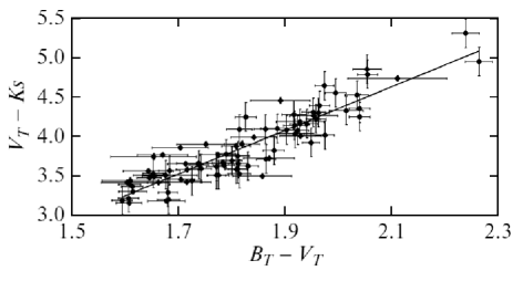
Figure 1: $(V_{T}-Ks)$ – $(B_{T}-V_{T})$ diagram for K-type RGB stars in the spatial cell with $0^{\circ}<l<90^{\circ}$, $-10^{\circ}<b<+10^{\circ}$, $200<r_{HIP}<300$ pc.

An example of the selection of stars of one class with similar spectra was given previously (Gontcharov 2011): the dereddened colors of 30 671 selected K-type RGB stars have a small scatter: $\sigma(V_{T}-Ks)_{0}=0.35^{m}$, $\sigma(B_{T}-V_{T})_{0}=0.08^{m}$. An example of determining the extinction law using these stars is presented in Fig. 1. The $(V_{T}-Ks)$ – $(B_{T}-V_{T})$ diagram is shown for K-type RGB stars in the spatial cell with coordinates $0^{\circ}<l<90^{\circ}$, $-10^{\circ}<b<+10^{\circ}$, $200<r_{HIP}<300$ pc, where $l$ is the Galactic longitude, $b$ is the Galactic latitude, and $r_{HIP}$ is the distance from Hipparcos parallaxes (ESA 1997; van Leeuwen 2007). The vertical and horizontal bars mark the formal accuracy of the photometry. The trend $(V_{T}-Ks)=2.76(B_{T}-V_{T})-1.17$ was drawn by the least-squares method. It may be concluded that $R_{V}=1.12\times 2.76=3.09$ in this spatial cell, which corresponds to the widespread “mean” or “standard” estimate.

Straizys (1977, pp. 39–40) called this the extinction law extrapolation method; Zasowski et al. 2009) called this the color ratio method. This method was apparently first applied by Jonhson and Borgman (1963). Unfortunately, as Wegner (2003) showed, this is the only direct method of determining $R_{V}$ using individual stars rather than, say, clusters applicable at present.

The difficulties in using the extinction law extrapolation method are the following.

• As has been shown above, a sample of stars with a similar spectral energy distribution, i.e., stars of the same spectral type, luminosity class, and metallicity, is needed to reduce the scatter of dereddened stellar colors. In addition, the peculiar stars and stellar pairs in which the photometry and spectra cannot be considered separately for each component should be excluded.

• The larger the range of stellar colors in the spatial cell under consideration, the more accurate the result (although the minimal scatter of dereddened colors is desirable!). Therefore, the method is applicable only in sufficiently large spatial cells, where the stars exhibit a wide range of colors as a result of their reddening and, in addition, the maximum reddening in such a cell is great. To be more precise, the method is applicable in a cell where the mean reddening is larger than the natural scatter of colors for unreddened stars and, in addition, the errors in the colors are larger due to the errors in the original photometry. For the stars used here, this is the region of space with $A_{V}>0.25^{m}$. Consequently, the method does not work within about 50 pc of the Sun. At high Galactic latitudes, as we show below in the results for RGB stars, the layer of absorbing matter above and below the Sun provides the necessary reddening and extinction $A_{V}\approx 0.3^{m}$.

• It follows from the aforesaid that the original photometry for the stars used must be fairly accurate. In any case, the colors must be determined with an accuracy that is a factor of $R_{V}$ higher than the mean level of $A_{V}$ in the spatial cell being investigated. The accuracy of the colors is at least $0.1^{m}$ – a level at which the method is efficient, while much more reliable results can be obtained at a photometric accuracy of $0.01^{m}$.

• The stars used must be sufficiently numerous. This is important not only for revealing and excluding peculiar stars but also because a large number of stars can to some extent compensate for the inaccuracy of the photometry. For example, nine stars in each spatial cell under consideration are needed to calculate $R_{V}\approx 3$ in the spatial cell with an accuracy of the original photometry at least $0.1^{m}$, i.e., with a relative accuracy of 3%. Consequently, 9000 uniformly distributed stars are needed to analyze $R_{V}$ in the sphere with a radius of 500 pc at a cell radius of 50 pc.

• To investigate the regions with large extinction, we must use high-luminosity stars seen from far away.

• To reduce the possible biases of the quantities being determined, the stars must be distributed fairly uniformly in space and the sample must be to a large extent complete to some distance.

Even the first application of the extinction law extrapolation method by Jonhson and Borgman (1963) allowed not only large deviations of $R_{V}$ from 3.1 for some stars but also a smaller (in amplitude) smooth dependence of $R_{V}$ on Galactic longitude with a minimum at $l\approx 110^{\circ}$ to be detected. However, as a result of the listed stringent requirements for the method, researchers adopt a certain constant (in the entire space) extinction law (for example, $R_{V}=3.1$), i.e., they assume the interstellar medium to be homogeneous with regard to the dust grain properties, despite progress in studying the reddening of stars. The maps of reddening variations obtained in this case are called “extinction maps”. However, when comparing such maps constructed from photometry at distinctly different wavelengths, there are discrepancies whose value apparently correlates with the dust temperature (Dutra et al. 2003; Peek and Graves 2010). The discrepancies between the reddening maps do not allow the spatial variations of the extinction law to be ignored any longer.

Previous Implementation of the Method

Various researchers have found that $R_{V}$ within the kiloparsec nearest to the Galactic center is considerably smaller than that near the Sun (Popowski 2000). However, only Sumi (2004) showed that this is not a local anomaly of the extinction law but possibly largescale variations within at least 1 kpc of the Galactic center: when recalculated, $R_{V}$ changes here along $l$ but not along $b$ approximately by 0.2 kpc^-1 if the stars being investigated are assumed to belong to a bar oriented at an angle of about 45^∘ to the Sun. In this case, the near part of the bar in the first Galactic quadrant shows a lower value of $R_{V}$ than its far part in the fourth quadrant and there is no extremum expected at the Galactic center. The grow of $R_{V}$ with increasing heliocentric distance toward the Galactic center is consistent with the results considered below, but extrapolating the results from Sumi (2004) to the circumsolar space gives too low values of $R_{V}$ and, in addition, the absence of an extremum at the center defies common sense. Thus, the results by Sumi (2004) require confirmation and analysis.

The large-scale spatial variations of the extinction law over at least 12 kpc were established more reliably by the extinction law extrapolation method and were analyzed in detail by Zasowski et al. (2009) based on a combination of 2MASS (three near-infrared bands) and Spitzer-IRAC (four mid-infrared bands) photometry for RGC stars. The seven photometric bands used cover the wavelength range from 1.2 to 8 microns. In this case, RGC stars near the Galactic plane in the bulk of the first and fourth Galactic quadrants farther than 10^∘ for the Galactic center (a total of 290 sq. deg. on the sky) in the range of magnitudes $11^{m}<J<15.5^{m}$. 5 were selected on the color–magnitude $(J-Ks)$ – $J$ diagram. Given $M_{J}\approx-1^{m}$ for RGC stars, they were selected at a heliocentric distance $2.5<r<15$ kpc, not including the region in the immediate vicinity of the Galactic center. The sky region under consideration was divided into $2.5^{\circ}\times 2^{\circ}$ cells, each containing from 820 to 60 000 selected stars. The colors with respect to the $H$ band like $(J-H)$, $(H-Ks)$, etc. were used for each star. For all stars in the cell, the linear dependence of the remaining colors with respect to $(H-Ks)$ was found by the least-squares method. The coefficient of this dependence characterizes the infrared extinction law and is related to $R_{V}$.

Systematic variations of the extinction law that gave, when recalculated, $R_{V}$ variations between 3.1 and 5.5 were found by Zasowski et al. (2009) in the Galactic region under consideration. The authors pointed out the inaccuracy of recalculating the result to $R_{V}$, because all of the previous absolute calibrations of the extinction law based on the medium s homogeneity are inapplicable. However, this inaccuracy is smaller than the variations found by several times. Since the longitude in the Galactic region being investigated strongly correlates with the Galactocentric distance, Zasowski et al. (2009) treat the longitude dependence of the extinction law as a dependence on the Galactocentric distance and, consequently, as a systematic decrease in the dust grain size and a decrease in nonselective extinction with increasing Galactocentric distance. Thus, dust of supermicron and submicron sizes apparently dominates in the central and outer Galactic regions, respectively. A correlation of the dust grain size with the stellar metallicity, the grain chemical composition and shape, and other parameters that can depend on the Galactocentric distance is also possible. Zasowski et al. (2009) point out that even excluding the known regions with anomalously large $R_{V}$ from consideration does not remove the systematic trend found. Thus, the $R_{V}$ variations were detected in much of the Galaxy and not only in one or more anomalous regions. This means that the $R_{V}$ variations are actually inherent in a diffuse medium, not in dense clouds, and these variations should not be confused with the well-known deviations of $R_{V}$ from 3.1 in small star-forming regions.

Applying a universal extinction law (for example, $R_{V}=3.1$) can give large systematic and random errors when calculating the extinctions, distances, absolute magnitudes, and other characteristics of stars in any Galactic region. These errors as a function of the error in $R_{V}$ were given by Reis and Corradi (2008): for variations within $R_{V}$ $\pm 1.5$ of the mean, the calculated distances and/or magnitudes of stars are in error by 10%. In this case, the systematic $R_{V}$ variations produce the systematic errors in the distances.

Zasowski et al. (2009) point out that the method of extrapolating the extinction law using only infrared photometry (without any visual bands) is applicable only in regions with a very large extinction: $E_{(J-Ks)}>0.35$, or $A_{V}>2^{m}$. In addition, it is inapplicable near the Sun due to the absence of accurate infrared photometry for bright stars (see Gontcharov 2011). Only a combination of infrared and visual photometry is possible within 1.5 kpc of the Sun.

Thus, the above peculiarities of the theory and the realization of the extinction law extrapolation method at present leave a very narrow choice of original material for investigating the variations of the extinction law within several hundred pc of the Sun: OB, RGC, and type-K RGB stars as numerous high-luminosity stars. The Tycho-2 catalog is the only source of their accurate visual photometry over the entire sky, while the 2MASS catalog serves as the only source of infrared photometry for such bright stars, although there are also other sources of photometry for analyzing the variations of the extinction law not over the entire sky but in individual regions.

ORIGINAL DATA

To analyze the variations of the extinction law, we use the $B_{T}$, $V_{T}$, and $Ks$ photometry as well as the trigonometric, $r_{HIP}$, and photometric, $r_{ph}$, distances separately for the samples of OB and type-K RGB stars. Our main goal is to detect consistent $R_{V}$ variations for so different classes of stars.

OB Stars

The sample of 37 485 OB stars was obtained previously (Gontcharov 2008a). To investigate the extinction in the Gould Belt, we excluded the stars with photometry poorer than $0.05^{m}$ at least in one of the bands used from the sample (Gontcharov 2009). In addition, the stars with an extinction exceeding $A_{V}=1.1/(0.25+|\sin(b)|)$, as a rule, late-type peculiar stars, were rejected. To increase the accuracy, we excluded the stars with known spectral classification from the Tycho Spectral Types catalogue (TST, Wright et al. 2003) that did not belong to the O, B, and A0 types from the sample. As a result (see Gontcharov 2009), the sample of 15 670 remaining OB stars was used. However, the spectral energy distribution for A0 stars differs noticeably from that for O and B ones. Therefore, for our study, we excluded the A0 stars according to the TST from the sample; 11 990 OB stars remained in our sample.

The median accuracy of $(B_{T}-V_{T})$ and $(V_{T}-Ks)$ is $0.03^{m}$. For all $\sigma(B_{T}-V_{T})<0.07^{m}$, $\sigma(V_{T}-Ks)<0.06^{m}$. Thus, the accuracy $\sigma(R_{V})<0.1$ in 99% of the spatial cells is achieved when only six OB stars are present in the cell. However, based on the available data, we cannot reliably exclude the giants, supergiants, Be stars, and stars with a peculiar spectrum, for which the reddening and extinction can differer from the normal ones, from the sample. To reduce the influence of these stars on the result, the spatial cells were chosen to have at least 25 stars in the cell. The high Galactic longitudes at which there are almost no OB stars constitute an exception. The method is also difficult to apply, because the mean reddening of the OB stars under consideration reaches an appreciable value, $\overline{E_{(B_{T}-V_{T})}}>0.1$, only at $|b|<50^{\circ}$. Therefore, when using spherical coordinates, the regions $b<-40^{\circ}$ and $b>+40^{\circ}$ were considered as two large indivisible spatial cells. When using rectangular $XYZ$ coordinates for the regions $50<|Z|<150$ pc at $\sqrt{X^{2}+Y^{2}}<300$ pc, we interpolated the results of the neighboring cells at the same $Z$ and did not consider the cells with $|Z|>150$. However, fairly reliable results were obtained for high latitudes from RGB stars.

For our study, we performed a new calibration of the absolute magnitude $M_{V_{T}}$ as a function of $(B_{T}-V_{T})_{0}$ based on 871 OB stars that, according to Hipparcos, are closer than 300 pc. In this case, $M_{V_{T}}=V_{T}+5-5\log(r_{HIP})-A_{V}$, where $A_{V}$ is the extinction calculated previously (Gontcharov 2008a). The $(B_{T}-V_{T})_{0}$ colors were obtained by correcting the original $(B_{T}-V_{T})$ for the reddening that was also calculated previously (Gontcharov 2008). Monte Carlo simulations (Gontcharov 2011) showed that the Malmquist and Lutz–Kelker biases may be neglected for so close stars.

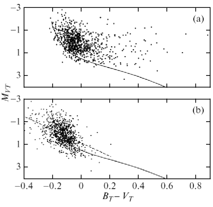
Figure 2: Distribution of 871 OB stars within 300 pc of the Sun on the $(B_{T}-V_{T})$ – $M_{V_{T}}$ diagram: (a) with the original $(B_{T}-V_{T})$, (b) with the dereddened $(B_{T}-V_{T})_{0}$. The solid and dashed curves represent the isochrone for solar-metallicity stars with an age of 60 Myr and the adopted calibration, respectively.

The distribution of these stars on the $(B_{T}-V_{T})$ – $M_{V_{T}}$ diagram is shown in Fig. 2: (a) with the original $(B_{T}-V_{T})$ and (b) with the dereddened $(B_{T}-V_{T})_{0}$. We see that the stars under consideration are noticeably reddened. Dereddening reduced the standard deviation from $\sigma(B_{T}-V_{T})=0.13^{m}$ to $\sigma((B_{T}-V_{T})_{0})=0.08^{m}$. and the mean from $\overline{(B_{T}-V_{T})}=0^{m}$ to $\overline{((B_{T}-V_{T})_{0}}=-0.13^{m}$ (for all 11 990 stars, these quantities are $\sigma(B_{T}-V_{T})=0.2^{m}$, $\sigma((B_{T}-V_{T})_{0})=0.09^{m}$, $\overline{(B_{T}-V_{T})}=0.15^{m}$, $\overline{((B_{T}-V_{T})_{0}}=-0.09^{m}$). These changes suggest that the calculated reddening is plausible. In addition, as has been noted above, the small $\sigma((B_{T}-V_{T})_{0})=0.08^{m}$, which does not exceed the mean reddening $\overline{E_{(B_{T}-V_{T})}}$ in the cells under consideration, is important for the method being applied.

The solid curve in Fig. 2 indicates the isochrone for solar-metallicity stars with an age of 60 Myr typical of late-OB stars calculated from the evolutionary models of Girardi et al. (2000) by taking into account the relations $(B_{T}-V_{T})=(B-V)/0.85$ and $M_{V_{T}}=M_{V}+0.09(B_{T}-V_{T})$ (ESA 1997). Given the errors of the original photometry, this isochrone fits well the bulk of the cloud of points after dereddening in Fig. 2b. However, the larger number of points above the isochrone suggests an admixture of giants in the sample. The positions of the extremely blue stars ($(B_{T}-V_{T})_{0}<-0.25$) are apparently explained by photometric errors. Both giants and photometric errors are inherent in the entire sample of 11 990 OB stars. They should be taken into account in the calibration. Therefore, we adopted an empirical calibration found by the least-squares method from data for 871 stars under consideration. It is indicated by the dashed line in Fig. 2b: $M_{V_{T}}=5.85(B_{T}-V_{T})_{0}+0.84$. The accuracy of the original photometry and parallaxes allows the accuracy of the coefficients found to be estimated as 5.85$\pm$0.05 and 0.84$\pm$0.05, respectively. The standard deviation for the stars relative to this calibration straight line is $\sigma(M_{V_{T}})=0.8$. This allows the photometric distances $\log(r_{ph})=(V_{T}-M_{V_{T}}+5-A_{V})/5$ to be calculated with a relative accuracy of 40%.

The photometric distances are important in our study, because the sample contains only 3606 Hipparcos stars (30%), the accuracy of $r_{HIP}$ is higher than 40% only for 1891 stars from them (16%). Thus, the sample of 11 990 under consideration is complete or almost complete in a much larger region of space (within 400 to 800 pc of the Sun, depending on b) than the sample of Hipparcos stars (150 to 300 pc, respectively), while the photometric distances for 84% of the sample stars are more accurate than the trigonometric ones. Therefore, below when considering the variations of the extinction law, the results using $r_{ph}$ are the main ones, while those with $r_{HIP}$ are considered only for checking.

Type-K RGB Stars

The sample of 30 671 K-type RGB stars was obtained previously (Gontcharov 2011). The median accuracy of $(B_{T}-V_{T})$ and $(V_{T}-Ks)$ is 0.03^m and 0.05^m, respectively. For 98% and 84% of the stars, $\sigma(B_{T}-V_{T})<0.1^{m}$ and $\sigma(V_{T}-Ks)<0.1^{m}$, respectively.

The absence of accurate near-infrared photometry for bright stars ($Ks<5.5^{m}$) in modern astronomy is a serious problem. For example, for the 2MASS project, these stars turned out to be too bright and, despite special efforts, even the formal accuracy of their photometry is, on average, lower than 0.3^m; actually, it can be even lower.

However, our cross-identification of the RGB stars under consideration using the SIMBAD database in Strasbourg showed that the IRAS satellite (IRAS 1988) measured the infrared flux at wavelengths of 12 and 25 microns for many of them. For stars with fairly accurate measurements of the $Ks$ magnitude and the 12-microns flux, these results were compared and a correlation was found: $Ks=0.0087(\log_{2.512}(F12))^{3})-0.0371(\log_{2.512}(F12))^{2})-0.95(\log_{2.512}(F12)))+4.2$, where $F12$ is the logarithm of the infrared flux at 12 microns to base 2.512. The scatter of $Ks$ magnitudes relative to this calibration curve for stars with accurate $Ks$ and $F12$ photometry is $\sigma(Ks)=0.18^{m}$. The calibration must give the same accuracy for stars with inaccurate $Ks$ photometry. Having applied this calibration to bright stars, we retain them in the sample.

Thus, the accuracy $\sigma(R_{V})<0.1$ is achieved everywhere when 36 K-type RGB stars are present in the cell. This condition can be fulfilled even for high Galactic latitudes. The type-K RGB stars have approximately the same $M_{V_{T}}$ as the OB stars considered. Therefore, the sample of K-type RGB stars is complete in the same space.

The photometric distances of the type-K RGB stars under consideration were calculated previously (Gontcharov 2011) with a relative error of 40%. The sample contains 9742 Hipparcos stars (32%); the accuracy of $r_{HIP}$ is higher than 40% only for 5401 stars from them (18%). Thus, $r_{ph}$ is more accurate than $r_{HIP}$ and the results using $r_{ph}$ are the main ones for 82% of the sample stars.

RESULTS

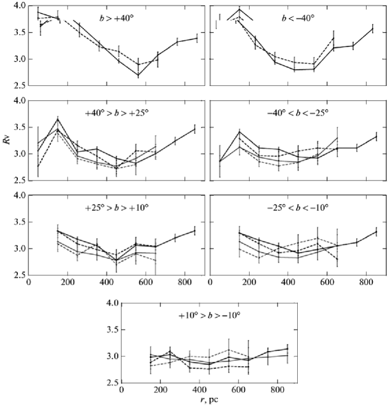
Figure 3: $R_{V}$ versus distance for various Galactic latitudes: the photometric and trigonometric distances of the RGB stars are indicated by the solid and dashed black lines, respectively; the photometric and trigonometric distances of the OB stars are indicated by the solid and dashed gray lines, respectively.

In Fig. 3, $R_{V}$ is plotted against the distance (with a 100-pc step) for various latitude zones. The results are indicated by the solid and dashed black lines for the RGB stars with $r_{ph}$ and $r_{HIP}$, respectively, and by the solid and dashed gray lines for the OB stars with $r_{ph}$ and $r_{HIP}$, respectively. The choice of the latitude zones is explained by the fact that the Gould Belt passes in the zone $10^{\circ}<|b|<25^{\circ}$ and its influence can manifest itself in the zone $25^{\circ}<|b|<40^{\circ}$, as was shown previously (Gontcharov 2009).

In contrast to the OB stars, the RGB stars at high latitudes ($|b|>40^{\circ}$) give fairly reliable results: the number of RGB stars here is great and the mean reddening $\overline{E_{(B_{T}-V_{T})}}=0.1^{m}$ is sufficient for the method to be applied.

The results for both classes of stars and both types of distances agree within the errors limits indicated by the vertical bars. This is an important result that shows that, despite significant random errors, the three independent distance scales (Hipparcos, RGB photometry, and OB photometry) are in good agreement in systematic terms. Below, we consider only the results with $r_{ph}$.

Systematic $R_{V}$ variations between 2.7 and 4.0. are seen at all latitudes. The minimum of $R_{V}$ is seen on all plots at a distance from 250 to 550 pc. The maximum of $R_{V}$ seen at a distance closer than 200 pc from the Sun grows with increasing distance from the Galactic equator. $R_{V}$ is almost constant along the Galactic equator. All of this suggests the presence of a vast, roughly symmetric (relative to the equator) and nearly spherical (in shape) structure in the solar neighborhood in which the dust grains are distributed nonuniformly in their sizes and/or other properties affecting $R_{V}$.

These systematic variations also manifest themselves when analyzing the data in rectangular $XYZ$ coordinates. In this case, $R_{V}$ was calculated from Eq. (1) for cells in the shape of a rectangular parallelepiped with height $Z=100$ pc and a square base the length of whose side (along $X$ or $Y$) was from 100 to 200 pc, so that there were at least 25 OB stars and at least 36 RGB stars in the cell. The calculations were performed by the moving average method: in each step, the parallelepiped was shifted by 20 pc along $X$ or $Y$ and $R_{V}$ was calculated for the stars in the parallelepiped by the least-squares method using Eq. (1). As a result, the calculations were performed in more than 200 000 cells. Although using a moving average slightly smoothed the results, it is quite justified, because the distance errors are a much more stronger smoothing factor (and the most important source of systematic errors).

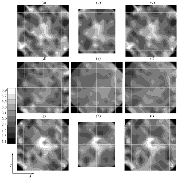
Figure 4: Contour maps of $R_{V}$ as a function of the $X$ and $Y$ coordinates: (a) RGB, $+50<Z<+150$ pc; (b) OB, $+50<Z<+150$ pc; (c) mean $R_{V}$, $+50<Z<+150$ pc; (d) RGB, $-50<Z<+50$ pc; (e) OB, $-50<Z<+50$ pc; (f) mean $R_{V}$, $-50<Z<+50$ pc; (g) RGB, $-150<Z<-50$ pc; (h) OB, $-150<Z<-50$ pc; (i) mean $R_{V}$, $-150<Z<-50$ pc. The gray scale for $R_{V}$ is shown on the left. The white lines of the coordinate grid are plotted with a 500-pc step. The Sun is at the centers of the plots; the Galactic center is on the right.

Figure 4 shows the contour maps of $R_{V}$ as a function of the $X$ and $Y$ coordinates for three layers along $Z$ for the RGB stars in the left column, for the OB stars in the middle column, and averaged for the two classes of stars in the right column: (a) RGB, $+50<Z<+150$ pc; (b) OB, $+50<Z<+150$ pc; (c) mean $R_{V}$, $+50<Z<+150$ pc; (d) RGB, $-50<Z<+50$ pc; (e) OB, $-50<Z<+50$ pc; (f) mean $R_{V}$, $-50<Z<+50$ pc; (g) RGB, $-150<Z<-50$ pc; (h) OB, $-150<Z<-50$ pc; (i) mean $R_{V}$, $-150<Z<-50$ pc. The gray scale for $R_{V}$ is given on the left. The isoline step is $\Delta R_{V}=0.2^{m}$. The white lines of the coordinate grid are plotted with a 500-pc step; the distance scale on all plots is the same. The Sun is at the centers of the plots; the Galactic center is on the right.

We see that the results for the two classes of stars agree well, although fewer details are seen in the $R_{V}$ variations for the OB stars, because we had to use large spatial cells (but with a side of no more than 200 pc, while the cell for the RGB stars is typically $100\times 100\times 100$ pc). The standard deviation of the “RGB minus OB” $R_{V}$ differences within 500 pc of the Sun is 0.2. This value may be considered an estimate of the accuracy of the method that was achieved using the data available to date. Obviously, the accuracy of the result can be increased significantly by increasing the accuracy of the photometry used and the distances. The achieved accuracy of determining $R_{V}$ (0.2) in the presence of $R_{V}$ variations at least between 2.7 and 4 leaves no doubt that these variations are real.

Below, we consider only the mean of the results for the RGB and OB stars.

In the equatorial layer ($-50<Z<+50$ pc), coarse dust dominates along the Great Tunnel, a structure formed by clouds and young stars (Gontcharov 2004; Gontcharov and Vityazev 2005) – the light-gray band extending on plot (f) from the top through the center to the lower left corner. The region of coarse dust, along with the Gould Belt, is inclined relative to the Galactic equator (by 17^∘; see Gontcharov 2009) and is located slightly northward of the equator toward the Galactic center (the Scorpius–Sagittarius region is seen as a light spot at the center of plot (c) in the first and fourth quadrants) and southward toward the anticenter (the Perseus–Orion region is seen as light spots on plot (i) in the second and third quadrants). The off-center position of the Sun relative to the Gould Belt and the region of coarse dust is also seen in the figure: the Scorpius–Sagittarius region with $r_{ph}\approx 100$ pc and the Orion region with $r_{ph}\approx 400$ pc.

In fact, the main feature of the $R_{V}$ variations within 500 pc of the Sun is the radial, relative to the Sun (to be more precise, apparently relative to the Local Bubble and the center of the Gould Belt), gradient in $R_{V}$ and, consequently, grain sizes. As we see from the figure, $R_{V}$ is minimal in the Local Bubble, a region of reduced gas density within about 100 pc of the Sun. As the heliocentric distance increases, $R_{V}$ rises sharply and reaches its maximum immediately outside the Local Bubble, at $r_{ph}\approx 100\div 150$ pc, in complete agreement with the result by Skorzynski et al. (2003), who detected a maximum of nonselective extinction here. Still farther from the center of this spherical structure, $R_{V}$ slowly decreases, reaching its minimum, in fact, at the edge of the Gould Belt, i.e., as has been shown above, at different heliocentric distances, for example, in the direction of Scorpius–Sagittarius and Perseus–Orion. Outside the Gould Belt, farther than 500 pc from the Sun, $R_{V}$ returns to its mean value.

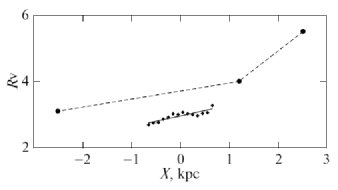
Figure 5: Dependence of $R_{V}$ on $X$ coordinate: obtained here when averaging the results in the layer $-50<Z<+50$ pc, $-500<Y<+500$ pc (the diamonds and solid line); obtained by Zasowski et al. (2009) (the circles and dashed line).

Apart from the variations associated with the Gould Belt, a gradual increase in $R_{V}$ toward the Galactic center, particularly in the equatorial layer, is noticeable (plot (f)). In Fig. 5, the diamonds and the solid line $R_{V}=0.3X+2.96$ indicate the dependence of $R_{V}$ of the $X$ coordinate (in kpc) when averaging the results in the layer $-50<Z<+50$, $-500<Y<+500$ pc. The dependence derived by Zasowski et al. (2009) is also indicated here by the circles and the dashed line. The vertical shift of the result by Zasowski et al. (2009) can be caused by the inaccuracy of the absolute calibrations of the infrared extinction law mentioned above. Good agreement between the revealed trends is important: 0.30 kpc^-1 in our study and 0.24 kpc^-1 in Zasowski et al. (2009). The trend found is not an artefact, because it does not manifest itself along $Y$ and $Z$. Thus, the conclusion reached by Zasowski et al. (2009) about the predominance of coarser dust at the Galactic center is confirmed.

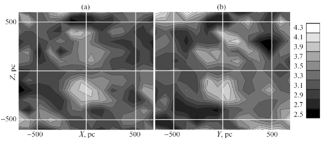
Figure 6: Contour maps of $R_{V}$ as a function of the coordinates: (a) $X$ and $Z$ for the layer $-150<Y<+150$ pc; (b) $Y$ and $Z$ for the layer $-150<X<+150$ pc. The gray scale for $R_{V}$ is given on the right. The white lines of the coordinate grid are plotted with a 500-pc step; the Sun is at the centers of the plots.

Figure 6 shows the contour maps of $R_{V}$ (the mean of the results for the RGB and OB stars) as a function of the coordinates: (a) $X$ and $Z$ for the layer $-150<Y<+150$ pc; (b) $Y$ and $Z$ for the layer $-150<X<+150$ pc. The gray scale for $R_{V}$ is given on the right. The white lines of the coordinate grid are plotted with a 500-pc step. the Sun is at the centers of the plots.

We see that the central (roughly equatorial) layer with a moderate $R_{V}\approx 3.2\div 3.4$ has a thickness corresponding to the traditional thickness estimates for the absorbing layer in the solar neighborhood – about 150 pc (Gontcharov 2009). This means that if $R_{V}$ is determined by the dust grain size, then it can be said that fine and coarse dust dominates where there is much and little dust, respectively. As in Figs. 3 and 4, systematic $R_{V}$ variations in the Gould Belt and its neighborhood manifest themselves here. In the $XZ$ plane on plot (a), the central layer with a moderate $R_{V}\approx 3.2\div 3.4$ is inclined to the Galactic equator just as the Gould Belt (the presence of this layer also proves that the detected spherical structure in the $R_{V}$ variations is not the artefact that resulted from the systematic errors in $r_{ph}$). The decrease in $R_{V}$ at $X\approx-600$ and $X\approx+250$ pc corresponds to the location of the Gould Belt edges. Two regions of extremely high $R_{V}$ clearly manifest themselves in this figure: two roughly hemispheres northward and southward of the Sun, with the northern one having a “defect” in the second quadrant – the region of lower $R_{V}$ independently pointed out by Fitzpatrick and Massa (2007). As the combination of Figs. 4 and 6 shows, there is the previously detected, also roughly spherical layer of minimum $R_{V}$ that also corresponds to the minima in Fig. 3 at the outer boundary of these hemispheres in all directions at a distance of about 500 pc from the Sun. Still farther from the Sun, $R_{V}$ returns to some mean value.

In general, the roughly radial (relative to the Sun) variations of the extinction law found can be caused by a systematic change in the composition of the samples of stars with heliocentric distance. However, the constancy of the normal $(B_{T}-V_{T})_{0}$ color for stars depending on the latitude, longitude, and distance that we verified proves the invariability of the composition of the samples.

It should be noted that there is no correlation, at least pronounced one, between $R_{V}$ and the reddening of stars: according to Gontcharov (2010), the reddening in the region under consideration is maximal in the first and second quadrants and has a deep minimum in the third one, while $R_{V}$ is maximal in the first and fourth quadrants and has a deep minimum in the second one. As has been noted above, this was detected long ago by Jonhson and Borgman (1963). The absence of a correlation between the reddening and $R_{V}$ also manifests itself in the fact that although the Gould Belt contains dense clouds causing the stars to redden (Gontcharov 2010), no $R_{V}$ variations have been in the direction of these clouds that would differ significantly from those in other directions.

CONCLUSIONS

This is the third paper in our series of studies of the interstellar extinction in the Galaxy. Our previous studies (Gontcharov 2009, 2010) showed that the stellar reddening and extinction could be analyzed using accurate multicolor broadband photometry from present-day surveys of millions of stars. In addition, these studies revealed a great role of the Gould Belt as a region containing absorbing matter and, in addition, oriented almost radially relative to the Sun.

Our investigation has shown that the hard-to-implement extinction law extrapolation method proposed about 50 years ago can be implemented at present in both infrared and visual spectral ranges, for example, using multicolor broadband photometry from the Tycho-2 and 2MASS catalogues for 11 990 OB and 30 671 K-type RGB stars and photometric distances. The values of $R_{V}$ obtained agree for the two classes of stars so that the standard deviation of the differences is 0.2. This accuracy level allows consistent (for the two classes of stars) systematic largescale variations of the extinction law and, accordingly, the ratio $R_{V}$ and the mean dust grain size within the nearest kiloparsec to be revealed with confidence. The detected $R_{V}$ variations between 2.2 and 4.4 not only manifest themselves in individual clouds but also span the entire space near the Sun, being related to the main Galactic structures of the nearest kiloparsec. In the Local Bubble within about 100 pc of the Sun, $R_{V}$ has a minimum. In the inner part of the Gould Belt and at high Galactic latitudes, at a distance of about 150 pc from the Sun, $R_{V}$ reaches a maximum and then decreases to its minimum in the outer part of the Belt and other directions at a distance of about 500 pc from the Sun, returning to its mean values far from the Sun.

Near the Galactic equator, we found a monotonic increase in $R_{V}$ by 0.3 per kpc toward the Galactic center that is consistent with the result obtained by Zasowski et al. (2009) for much of the Galaxy.

We showed that ignoring the $R_{V}$ variations and traditionally using a single value for the entire space should lead to systematic errors in the calculated distances reaching 10%. In addition, the detection of such large $R_{V}$ variations forces us to recalculate the data of the numerous reddening and extinction maps obtained in recent years from the photometry of millions of stars.

The dependences of $R_{V}$ on the reddening, extinction, spectral type, and other characteristics of stars found by various researchers (Straizys 1977) are not fully explained by the theory of the method under consideration. The consistency of the $R_{V}$ variations for red giants and OB stars found here suggests that many of these dependences, if not all, are the artifacts that resulted from the disregarded correlations between the stellar characteristics and $R_{V}$ variations.

In this study, we independently confirm the radial (relative to the Sun) orientation of the absorbing matter within the nearest kiloparsec found previously (Gontcharov 2010). The Local Bubble and the central region of the Gould Belt located near the Sun seem to be actually the center here. This, along with the detection of regions with extremely large $R_{V}$ and, hence, large nonselective extinction at high latitudes, is of great importance for estimating the extinction toward extragalactic objects and the mass of the baryonic dark matter.

This paper may be considered as groundwork at the beginning of extensive studies, primarily as a proof of the necessity of investigating the large-scale variations of the extinction law. Analysis of the difficulties in applying the extinction law extrapolation method revealed not only its great potential but also the need for original data of a completely different level. At present, there is no accurate infrared photometry for bright stars and visual all-sky photometry for stars fainter than $11^{m}$. Only the largest-scale variations of the extinction law and only within about 500 pc of the Sun can be revealed by applying the method to tens of thousands of stars. At the same time, our investigation showed that the influence of the Gould Belt and other local structures disappears only beyond this radius and precisely the Galactic variations of the extinction law can at last manifest themselves. Complete samples of stars within several kpc of the Sun (i.e., samples of tens of millions of stars to $18^{m}$) are needed for their serious analysis.

The number of stars is particularly small at high latitudes, precisely where the most interesting results, especially important for extragalactic astronomy and dark matter studies, are evident. As a result, the mean accuracy of the photometry in a spatial cell at high latitudes barely exceeds the reddening. This does not allow the final conclusions to be reached. Since the layer of OB stars is thin, the extinction law at high latitudes can apparently be investigated only by using red giants.

Thus, not only the parallaxes from the Gaia project but also the reconstruction of the entire complex wavelength dependence of extinction in each spatial cell are needed to construct an accurate three-dimensional map for the variations of the extinction law in much of the Galaxy. In turn, this requires multiband photometry (in fact, spectrophotometry) with an accuracy of at least 0.01^m in the ultraviolet, visual, and infrared ranges for tens of millions of red giants with $0^{m}<V<18^{m}$ over the entire sky.

References

- 1. R. Drimmel, A. Cabrera-Lavers, M. Lopez-Corredoira, Astron. Astrophys. 409, 205, (2003).
- 2. C.M. Dutra, B.X. Santiago, E.L.D. Bica, B. Barbuy, Mon. Not. R. Astron. Soc. 338, 253, (2003).
- 3. ESA, Hipparcos and Tycho catalogues (ESA, 1997).
- 4. E.L. Fitzpatrick, Publ. Astron. Soc. Pacif. 111, 63, (1999).
- 5. E.L. Fitzpatrick and D. Massa, Astrophys. J. 663, 320, (2007).
- 6. E.L. Fitzpatrick and D. Massa, Astrophys. J. 699, 1209, (2009).
- 7. L. Girardi, A. Bressan, G. Bertelli, et al., Astron. Astrophys. Suppl. Ser. 141, 371, (2000), http://stev.oapd.inaf.it/YZVAR/.
- 8. G.A. Gontcharov, Astron. Soc. Pacif. Conf. Proc., 316, c. 221 (2004).
- 9. G. A. Gontcharov, Astron. Lett. 34, 7, (2008a).
- 10. G. A. Gontcharov, Astron. Lett. 34, 785, (2008b).
- 11. G. A. Gontcharov, Astron. Lett. 35, 780, (2009).
- 12. G. A. Gontcharov, Astron. Lett. 36, 584, (2010).
- 13. G. A. Gontcharov, Astron. Lett. 37, 707, (2011).
- 14. G. A. Gontcharov and V. V. Vityazev, Vestn. SPbGU, Ser. 1 3, 127 (2005).
- 15. E. Høg, C. Fabricius, V.V. Makarov, et al., Astron. Astrophys. 355, L27, (2000).
- 16. IRAS working group), IRAS Catalog of Point Sources, Version 2.0 (IRAS, 1988), http://cdsarc.u-strasbg.fr/viz-bin/Cat?II/125.
- 17. H.L. Jonhson and J. Borgman, Bull. Astron. Inst. Netherlands 17, 115, (1963).
- 18. F. van Leeuwen, Astron. Astrophys. 474, 653, (2007).
- 19. D. Moro, U. Munari, Astron. Astrophys. Suppl. Ser. 147, 361, (2000).
- 20. J.E.G. Peek and G.J. Graves, Astrophys. J. 719, 415, (2010).
- 21. M. Perryman, Astronomical application of astrometry (Cambridge Univ. Press, Cambridge, 2009).
- 22. A.J. Pickles, Publ. Astron. Soc. Pacif. 110, 863, (1998).
- 23. Popowski P., Astrophys. J. 528, L9, (2000).
- 24. W. Reis and W.J.B. Corradi, Astron. Astrophys. 486, 471, (2008).
- 25. W. Skorzynski, A. Strobel, G. Galazutdinov, Astron. Astrophys. 408, 297, (2003).
- 26. M.F. Skrutskie, R.M. Cutri, R. Stiening, et al., Astron. J. 131, 1163, (2006), http://www.ipac.caltech.edu/2mass/releases/allsky/index.html.
- 27. V. L. Straizys, Multicolor Stellar Photometry (Mosklas, Vil nyus, 1977; Pachart Publ., Tucson, 1992).
- 28. J. Sudzius and S. Raudeliunas, Baltic Astron. 12, 520, (2003).
- 29. T. Sumi, Mon. Not. R. Astron. Soc. 349, 193, (2004).
- 30. W. Wegner, Astron. Nachr. 324, 219, (2003).
- 31. C.O. Wright, M.P. Egan, K.E. Kraemer, et al., Astron. J. 125, 359, (2003).
- 32. G. Zasowski, S.R. Majewski, R. Indebetouw, et al., Astrophys. J. 707, 510, (2009).