Integration-by-parts reductions from unitarity cuts and algebraic geometry

Abstract:

Integration-by-parts reductions play a central role in perturbative QFT calculations. They allow the set of Feynman integrals contributing to a given observable to be reduced to a small set of basis integrals, and they moreover facilitate the computation of those basis integrals. We introduce an efficient new method for generating integration-by-parts reductions. This method simplifies the task by making use of generalized-unitarity cuts and turns the problem of finding the needed total derivatives into one of solving certain polynomial (so-called syzygy) equations.

1 Introduction

Precise predictions of the production cross sections at the Large Hadron Collider are necessary to gain a quantitative understanding of the Standard Model signals and background. To match the experimental precision and the parton distribution function uncertainties, this typically requires computations at next-to-next-to leading order in fixed-order perturbation theory. Calculations at this order are challenging due to the large number of contributing Feynman diagrams, involving loop integrals with high powers of loop momenta in the numerator of the integrand.

A key tool in these computations are integration-by-parts (IBP) identities [1, 2]. These are relations that arise from the vanishing integration of total derivatives. Schematically, they take the form,

$$\int\prod_{i=1}^{L}\frac{{\rm d}^{D}\ell_{i}}{\pi^{D/2}}\sum_{j=1}^{L}\frac{\partial}{\partial\ell_{j}^{\mu}}\frac{v_{j}^{\mu}\hskip 1.42262ptP}{D_{1}^{a_{1}}\cdots D_{k}^{a_{k}}}\hskip 2.84526pt=\hskip 2.84526pt0\,,$$ (1)

where $P$ and the vectors $v_{j}^{\mu}$ are polynomials in the internal and external momenta, the $D_{k}$ denote inverse propagators, and $a_{i}\geq 1$ are integers. In practice, the IBP identities generate a large set of linear relations between loop integrals, allowing a significant fraction to be reexpressed in terms of a finite basis of integrals. (The fact that the basis of integrals is always finite was proven in ref. [3].) The latter step of solving the linear systems arising from eq. (1) may be done by Gauss-Jordan elimination in the form of the Laporta algorithm [4, 5], leading in general to relations involving integrals with squared propagators. There are several publically available implementations of automated IBP reduction: AIR [6], FIRE [7, 8], Reduze [9, 10], LiteRed [11], in addition to private implementations. An approach for deriving IBP reductions without squared propagators was developed in ref. [12]. A recent approach [13] uses numerical sampling of finite-field elements to construct the reduction coefficients.

In addition to reducing the contributing Feynman diagrams to a small set of basis integrals, the IBP reductions provide a way to compute these integrals themselves via differential equations [14, 15, 16, 17, 18, 19, 20]. Letting $x_{m}$ denote a kinematical variable, $\epsilon=\frac{4-D}{2}$ the dimensional regulator, and $\boldsymbol{\mathcal{I}}(\boldsymbol{x},\epsilon)=\big{(}\mathcal{I}_{1}(\boldsymbol{x},\epsilon),\ldots,\mathcal{I}_{N}(\boldsymbol{x},\epsilon)\big{)}$ the basis of integrals, the result of differentiating a basis integral wrt. $x_{m}$ can be written as a linear combination of the basis integrals by using, in practice, the IBP reductions. As a result, one has a linear system of differential equations,

$$\frac{\partial}{\partial x_{m}}\boldsymbol{\mathcal{I}}(\boldsymbol{x},\epsilon)=A_{m}(\boldsymbol{x},\epsilon)\boldsymbol{\mathcal{I}}(\boldsymbol{x},\epsilon)\,,$$ (2)

which, supplied with appropriate boundary conditions, can be solved to yield expressions for the basis integrals. This method has proven to be a powerful tool for computing two- and higher-loop integrals. IBP reductions thus play a central role in perturbative calculations in particle physics.

In many realistic multi-scale problems, such as $2\to n$ scattering amplitudes with $n\geq 2$, the step of generating IBP reductions with existing algorithms is the most challenging part of the calculation. It is therefore interesting to explore other approaches to generating these reductions.

In these proceedings, based on ref. [21], we explain how IBP reductions can be obtained efficiently by applying a set of unitarity cuts dictated by a specific set of subgraphs and solving associated polynomial (syzygy) equations. A similar approach was introduced by Harald Ita in ref. [22] where IBP relations are also studied in connection with cuts, and their underlying geometric interpretation is clarified.

2 Setup

Throughout these proceedings, we will focus on the case of two-loop integrals. We will denote the number of external legs of a given two-loop integral by $n$, and the number of propagators by $k$. (Note that, after integrand reduction, $k\leq 11$.) We work in dimensional regularization and use the four-dimensional helicity scheme, taking the external momenta in four dimensions.

Our first aim is to recast two-loop integrals in a parametrization which is useful for deriving IBP relations. The first step is to decompose the loop momenta into four- and $(D-4)$-dimensional parts, $\ell_{i}=\overline{\ell}_{i}+\ell_{i}^{\perp}$, $i=1,2$. Next, parametrize the extra-dimensional vectors $\ell_{i}^{\perp}$ in hyperspherical coordinates, using their norms $\mu_{ii}\equiv-(\ell_{i}^{\perp})^{2}\geq 0$ and relative angle $\mu_{12}\equiv-\ell_{1}^{\perp}\cdot\ell_{2}^{\perp}$. After this transformation, the two-loop integral takes the form

$$I^{(2)}_{n\geq 5} =\frac{2^{D-6}}{\pi^{5}\Gamma(D-5)}\int_{0}^{\infty}{\rm d}\mu_{11}\int_{0}^{\infty}{\rm d}\mu_{22}\int_{-\sqrt{\mu_{11}\mu_{22}}}^{\sqrt{\mu_{11}\mu_{22}}}{\rm d}\mu_{12}\big{(}\mu_{11}\mu_{22}-\mu_{12}^{2}\big{)}^{\frac{D-7}{2}}\int{\rm d}^{4}\overline{\ell}_{1}\hskip 1.42262pt{\rm d}^{4}\overline{\ell}_{2}\frac{P(\ell_{1},\ell_{2})}{D_{1}\cdots D_{k}}\,.$$ (3)

For $n\geq 5$ there are $11-k$ irreducible scalar products (ISPs) which we denote by $g_{j}$ where $j=1,\ldots,11-k$. We can then define variables $z_{1},\ldots,z_{11}$ as follows,

$$z_{i}\equiv\left\{\begin{array}[]{lrl}D_{i}&1\leq&i\leq k\\[2.84526pt] g_{i-k}&k+1\leq&i\leq m\,,\end{array}\right.$$ (4)

with $m=11$ for $n\geq 5$. The transformation $\{\bar{\ell}_{i},\mu_{ij}\}\rightarrow\{z_{1},\ldots,z_{11}\}$ is invertible, with a polynomial inverse (provided the $g_{j}$ are chosen to take the form $\frac{1}{2}(\ell_{i}+K_{j})^{2}$, rather than linear dot products of the $\ell_{i}$), and has a constant Jacobian. The integral (3) then becomes,

$$I^{(2)}_{n\geq 5}=\frac{2^{D-6}}{\pi^{5}\Gamma(D-5)J}\int\prod_{i=1}^{11}{\rm d}z_{i}\hskip 1.70717ptF(z)^{\frac{D-7}{2}}\frac{P(z)}{z_{1}\cdots z_{k}}\,,$$ (5)

where $F(z)$ denotes the kernel $(\mu_{11}\mu_{22}-\mu_{12}^{2})$ expressed in the $z_{i}$, in which it is polynomial.

The representation (5) is valid for $n\geq 5$ external legs. For lower multiplicities, the loop momenta have components which can be integrated out before the transformation (4) is applied. For example, for $n=4$, by momentum conservation, there are only three linearly independent external momenta, and we can find an orthogonal vector $\omega$; that is, $p_{i}\cdot\omega=0$ where $i=1,\ldots,4$. Integrating out the components $\ell_{i}\cdot\omega$ in eq. (3) and subsequently applying the transformation (4) yields,

$$I^{(2)}_{n=4}=\frac{2^{D-5}}{\pi^{4}\Gamma(D-4)J}\int\prod_{i=1}^{9}{\rm d}z_{i}\hskip 1.70717ptF(z)^{\frac{D-6}{2}}\frac{P(z)}{z_{1}\cdots z_{k}}\,.$$ (6)

We observe that the spacetime dimensions appearing here have been shifted down by one relative to eq. (5); that is, $D-D_{c}\to D-(D_{c}-1)$. This is consistent with the fact that the span of the external momenta has one dimension less. For notational convenience we will drop the prefactors in front of the integral signs in eqs. (5) and (6). We note that the representations (5) and (6) have also been considered in the literature by Baikov, see for example ref. [23].

3 Integration-by-parts reductions on generalized-unitarity cuts

The key idea of our approach is to derive IBP identities on generalized-unitarity cuts where some subset $S$ of propagators are put on shell: $D_{i}^{-1}\to\delta(D_{i})$ with $i\in S$. In essence, the application of cuts divide the task of finding IBP reductions into several smaller, and more manageable, problems. This is because, on a given cut $S$, only integrals which contain all of the propagators in $S$ contribute (since the remaining integrals are missing the pole whose residue the cut is computing). As the resulting IBP identities will miss contributions from some of the basis integrals, we must construct the identities on a set of cuts $S_{1},\ldots,S_{C}$ and merge the partial results. Below we explain how to construct IBP identities on a given cut $S$ and how to choose an appropriate spanning set of cuts.

Let us consider a cut where $c$ propagators are put on shell ($0\leq c\leq k$). We label the propagators of the graph (cf. the labelling, e.g., in Fig. 1) and let $\mathcal{S}_{\mathrm{cut}}$, $\mathcal{S}_{\mathrm{uncut}}$ and $\mathcal{S}_{\mathrm{ISP}}$ denote the sets of indices labelling cut propagators, uncut propagators and ISPs, respectively. $\mathcal{S}_{\mathrm{cut}}$ thus contains $c$ elements. Furthermore, we let $m$ denote the total number of $z_{j}$ variables, and set $\mathcal{S}_{\mathrm{uncut}}=\{r_{1},\ldots,r_{k-c}\}$ and $\mathcal{S}_{\mathrm{ISP}}=\{r_{k-c+1},\ldots,r_{m-c}\}$. Then, after cutting the propagators, $z_{i}^{-1}\to\delta(z_{i}),i\in\mathcal{S}_{\mathrm{cut}}$, the integrals (5) and (6) reduce to,

$$I^{(2)}_{\mathrm{cut}}=\int\frac{{\rm d}z_{r_{1}}\cdots{\rm d}z_{r_{m-c}}P(z)}{z_{r_{1}}\cdots z_{r_{k-c}}}F(z)^{\frac{D-h}{2}}\bigg{|}_{z_{i}=0\,,\forall i\in\mathcal{S}_{\mathrm{cut}}}\,,$$ (7)

where $h$ depends on the number of external legs: $h=6$ for $n=4$ and $h=7$ for $n\geq 5$.

Now we turn to the problem of writing down IBP relations. An IBP relation (1) that concerns integrals with $m$ integration variables corresponds to a total derivative, or equivalently an exact differential form, of degree $m$. Here we are interested in the $c$-fold cut of the IBP relation, where the propagators of $\mathcal{S}_{\mathrm{cut}}$ are put on shell in all terms (and integrals which do not contain all of these propagators are set to zero). Such $c$-fold cut relations correspond to exact differential forms of degree $m-c$. The generic exact form that matches the form of the integrand in eq. (7) is,

$$0=\int{\rm d}\bigg{(}\sum_{i=1}^{m-c}\frac{(-1)^{i+1}a_{r_{i}}F(z)^{\frac{D-h}{2}}}{z_{r_{1}}\cdots z_{r_{k-c}}}{\rm d}z_{r_{1}}\wedge\cdots\wedge\widehat{{\rm d}z_{r_{i}}}\wedge\cdots\wedge{\rm d}z_{r_{m-c}}\bigg{)}$$ (8)

where the $a_{i}$’s are polynomials in $\{z_{r_{1}},\ldots,z_{r_{m-c}}\}$. (Similar differential form ansätze for four-dimensional IBPs on cuts were considered in ref. [24].) Writing out eq. (8) more explictly, we get the IBP relation,

$$0=\int\bigg{(}\sum_{i=1}^{m-c}\Big{(}\frac{\partial a_{r_{i}}}{\partial z_{r_{i}}}+\frac{D-h}{2F}a_{r_{i}}\frac{\partial F}{\partial z_{r_{i}}}\Big{)}-\sum_{i=1}^{k-c}\frac{a_{r_{i}}}{z_{r_{i}}}\bigg{)}\frac{F(z)^{\frac{D-h}{2}}}{z_{r_{1}}\cdots z_{r_{k-c}}}{\rm d}z_{r_{1}}\wedge\cdots\wedge{\rm d}z_{r_{m-c}}\,.$$ (9)

Now, for generic $a_{i}$, the second term in the sum corresponds to an integrand in $(D-2)$ dimensions. This is because the factor $F$ in the denominator divides against the integration measure $F(z)^{\frac{D-h}{2}}$ and thereby shifts $D\to D-2$ in the exponent. Likewise, the third term generates integrals with doubled propagators. To get an IBP relation that involves only integrals in $D$ dimensions with single-power propagators, we require the $a_{i}$ to be such that the second and third terms of (9) are polynomial rather than rational,

$$bF+\sum_{i=1}^{m-c}a_{r_{i}}\frac{\partial F}{\partial z_{r_{i}}} =0$$ (10)

$$a_{r_{i}}+b_{r_{i}}z_{r_{i}} =0\,,\hskip 11.38109pti=1,\ldots,k-c\,,$$ (11)

where $a_{r_{i}}$, $b$ and $b_{r_{i}}$ must be polynomials in $z_{j}$. Equations of this type are known in algebraic geometry as syzygy equations. They have been considered in the context of IBP relations in refs. [12, 25, 22]. In practice, the equations (10)–(11) can be solved with computational algebraic geometry software, such as Singular [26]. The corresponding IBP identities are then obtained by plugging the solutions into eq. (9). In this way, we find IBP identities on the cut $\mathcal{S}_{\mathrm{cut}}$.

To find an appropriate set of cuts on which to reconstruct the IBP reductions, we first find a basis of integrals. We perform this step without applying cuts and using rational numbers or finite-field element values for the kinematical invariants and spacetime dimension. Applying Gauss-Jordan elimination to the resulting set of IBP identities with some chosen ordering on the set of integrals then produces a basis of integrals. (Similar ideas for finding a basis of integrals have appeared in ref. [27], using random prime numbers for the external invariants and spacetime dimension, and in ref. [28], using finite-field elements.) In the example in the next section we explain how the set of cuts is obtained from the basis of integrals. Having obtained an appropriate set of cuts, we proceed analytically and construct IBP reductions on each cut in turn. Finally, we merge the results obtained from the cuts to find complete IBP reductions.

4 Example

To demonstrate the method, we consider the example of a planar double-box integral with all legs and propagators massless, illustrated in Fig. 1. For this integral we have $k=7$, and the inverse propagators can be parametrized as,

$$D_{1} =\ell_{1}^{2}\,,\quad D_{2}=(\ell_{1}-p_{1})^{2}\,,\quad D_{3}=(\ell_{1}-p_{1}-p_{2})^{2}$$

$$D_{4} =(\ell_{2}-p_{3}-p_{4})^{2}\,,\quad D_{5}=(\ell_{2}-p_{4})^{2}\,,\quad D_{6}=\ell_{2}^{2}\,,\quad D_{7}=(\ell_{1}+\ell_{2})^{2}\,.$$ (12)

As mentioned above eq. (4), the generic integral of this topology will have numerator insertions which are monomials in two distinct ISPs. The ISPs may be chosen as,

$$D_{8}=\frac{1}{2}(\ell_{1}+p_{4})^{2},\quad D_{9}=\frac{1}{2}(\ell_{2}+p_{1})^{2}\,.$$ (13)

Our aim is now to show how the IBP reductions of an integral with the propagators in eq. (12) with a generic numerator insertion can be obtained. After the change of variables $\{\bar{\ell}_{i},\mu_{ij}\}\rightarrow\{z_{1},\ldots,z_{9}\}$ discussed in section 2, the double-box integral takes the form of eq. (6).

We will use the following notation for the integrals,

$$G[n_{1},\ldots,n_{9}]\equiv\int\prod_{i=1}^{9}{\rm d}z_{i}\hskip 1.70717ptF(z)^{\frac{D-6}{2}}z_{1}^{n_{1}}\cdots z_{9}^{n_{9}}\,.$$ (14)

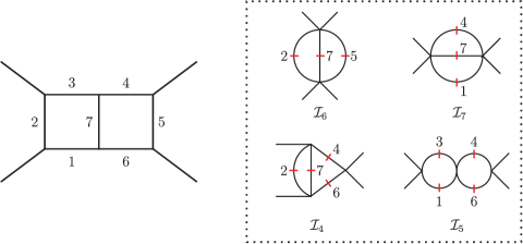
Figure 1: The massless double-box diagram, along with our labelling conventions for its internal lines, is shown on the left. The right part shows the subset of the master integrals in eq. (15) with the property that their graphs cannot be obtained by adding internal lines to the graph of some other master integral. The corresponding cuts $\{2,5,7\}$, $\{1,4,7\}$, $\{2,4,6,7\}$ and $\{1,3,4,6\}$ are the cuts required for deriving complete IBP relations of integrals with this double-box topology.

Now, to find the IBP reductions of these integrals, the first step is to find a basis of integrals. This is done by solving the syzygy equations (10)–(11) without imposing cuts while using numerical external kinematics (with rational numbers or finite-field elements), and then inserting all solutions into the right-hand side of eq. (9), and finally performing Gauss-Jordan elimination with some chosen ordering on the set of integrals. In the case at hand, we find the following set of master integrals (after modding out by symmetries)

$$\begin{array}[]{rl}\mathcal{I}_{1}&\equiv G[-1,-1,-1,-1,-1,-1,-1,0,0]\\ \mathcal{I}_{2}&\equiv G[-1,-1,-1,-1,-1,-1,-1,1,0]\\ \mathcal{I}_{3}&\equiv G[0,-1,-1,0,-1,-1,-1,0,0]\\ \mathcal{I}_{4}&\equiv G[0,-1,0,-1,0,-1,-1,0,0]\\ \mathcal{I}_{5}&\equiv G[-1,0,-1,-1,0,-1,0,0,0]\\ \mathcal{I}_{6}&\equiv G[0,-1,0,0,-1,0,-1,0,0]\\ \mathcal{I}_{7}&\equiv G[-1,0,0,-1,0,0,-1,0,0]\\ \mathcal{I}_{8}&\equiv G[-1,-1,-1,0,-1,0,-1,0,0]\,.\end{array}$$ (15)

Having obtained a basis of integrals, we proceed to find the IBP reductions analytically on a set of cuts and then merging the results to find the complete reductions. To decide on the minimal set of cuts required, we select those basis integrals with the property that their graphs cannot be obtained by adding internal lines to the graph of some integral in the basis. In the present case, this subset is $\{\mathcal{I}_{4},\mathcal{I}_{5},\mathcal{I}_{6},\mathcal{I}_{7}\}$, shown in Fig. 1. Hence, we only need to consider the four cuts $\{2,5,7\}$, $\{1,4,7\}$, $\{2,4,6,7\}$ and $\{1,3,4,6\}$ to find the complete IBP reductions.

To illustrate how to find the IBP reductions on a given cut, let us consider the three-fold cut $\mathcal{S}_{\mathrm{cut}}=\{2,5,7\}$. Here, $\mathcal{S}_{\mathrm{uncut}}=\{1,3,4,6\}$ and $\mathcal{S}_{\mathrm{ISP}}=\{8,9\}$. The kernel $F$ on the cut is polynomial in $z_{1}$, $z_{3}$, $z_{4}$, $z_{6}$, $z_{8}$ and $z_{9}$. The syzygy equations (10)–(11) read,

$$bF\hskip 1.42262pt+\sum_{i\in\{1,3,4,6,8,9\}}a_{i}\frac{\partial F}{\partial z_{i}}=0\hskip 25.60747pt\mathrm{and}\hskip 25.60747pta_{j}+b_{j}z_{j}=0\,,\hskip 8.53581ptj\in\{1,3,4,6\}\,,$$ (16)

where $b,b_{i},a_{j}$ are to be solved for as polynomials in $z_{k}$. A generating set of solutions of eq. (16) can be found via algebraic geometry software such as Singular in seconds (with analytic coefficients). Now, given a solution $(b,b_{i},a_{j})$, any multiple $(qb,qb_{i},qa_{j})$, with $q$ a polynomial, is manifestly also a solution. To capture the IBP reductions of all possible numerator insertions, we thus consider all syzygies $(b,b_{i},a_{j})$ multiplied by appropriate monomials in the ISPs, $q=\prod_{i\in\{1,3,4,6,8,9\}}D_{i}^{a_{i}}$. Inserting all such solutions into the right-hand side of eq. (9) produces the complete set of IBP relations, without doubled propagators, on the cut $\{2,5,7\}$ (i.e., up to integrals that vanish on this cut).

As an example, consider the tensor integral $T\equiv G[-1,-1,-1,-1,-1,-1,-1,0,2]$. On the four cuts specified above this integral reduces to, respectively,

$$T\big{|}_{\{2,5,7\}} =\sum_{j\in\{1,2,3,6,8\}}c_{j}\mathcal{I}_{j}\,,\hskip 17.07164ptT\big{|}_{\{1,4,7\}}=\sum_{j\in\{1,2,7\}}c_{j}\mathcal{I}_{j}\,,$$ (17)

$$T\big{|}_{\{2,4,6,7\}} =\sum_{j\in\{1,2,4\}}c_{j}\mathcal{I}_{j}\,,\hskip 17.07164ptT\big{|}_{\{1,3,4,6\}}=\sum_{j\in\{1,2,5\}}c_{j}\mathcal{I}_{j}\,,$$ (18)

where, denoting $\chi\equiv t/s$, the coefficients are found to be,

$$c_{1} =\frac{(D-4)s^{2}\chi}{8(D-3)}\,,\hskip 22.76219ptc_{2}=-\frac{(3D-2\chi-12)s}{4(D-3)}\,,\hskip 22.76219ptc_{3}=\frac{(4-D)(9\chi+7)}{4(D-3)}$$ (19)

$$c_{4} =\frac{(10-3D)(2\chi-13)}{8(D-4)s}\,,\hskip 22.76219ptc_{5}=\frac{2D(\chi+1){-}8\chi{-}7}{2(D-4)s}\,,\hskip 22.76219ptc_{6}=\frac{9(3D{-}10)(3D{-}8)}{4(D-4)^{2}s^{2}\chi}$$ (20)

$$c_{7} =\frac{(3D-10)(3D-8)(2\chi+1)}{2(D-4)^{2}(D-3)s^{2}}\,,\hskip 22.76219ptc_{8}=2\,.$$ (21)

The integrals absent from the right-hand sides of eqs. (17)–(18) vanish on the respective cuts. Combining these results, we get the complete IBP reduction of the tensor integral,

$$T=\sum_{j=1}^{8}c_{j}\mathcal{I}_{j}\,.$$ (22)

We have implemented the algorithm as a program, powered by Mathematica and Singular [26]. It analytically reduces all integrals with numerator rank $\leq 4$, to the eight master integrals in eq. (15) in about $39$ seconds in the fully massless case, and to $19$ master integrals in about $162$ seconds in the one-massive-particle case (on a laptop with 2.5 GHz Intel Core i7 and 16 GB RAM).

One important feature of the approach is the use of the $z_{i}$-variables in eq. (4) which ultimately lead to the simple form of the syzygy equations (10)–(11). However, the crucial feature is the use of generalized-unitarity cuts: they eliminate variables in the syzygy equations so that these can be solved more efficiently. More importantly, because on any given cut, only a subset of basis integrals contribute, the cuts have the effect of “block-diagonalizing” the linear system of IBP identities on which Gauss-Jordan elimination is performed to find the IBP reductions.

There are several directions for future research. Of particular interest are extensions to higher multiplicity, several external and internal masses, non-planar diagrams, and higher loops.

Acknowledgments

We thank S. Badger, H. Frellesvig, E. Gardi, A. Georgoudis, A. Huss, H. Ita, D. Kosower, A. von Manteuffel, M. Martins, C. Papadopoulos and R. Schabinger for useful discussions. The research leading to these results has received funding from the European Union Seventh Framework Programme (FP7/2007-2013) under grant agreement no. 627521, and Swiss National Science Foundation (Ambizione PZ00P2_161341).

References

- [1] F. V. Tkachov, Phys. Lett. B100, 65 (1981).
- [2] K. G. Chetyrkin and F. V. Tkachov, Nucl. Phys. B192, 159 (1981).
- [3] A. V. Smirnov and A. V. Petukhov, Lett. Math. Phys. 97, 37 (2011), 1004.4199.
- [4] S. Laporta, Phys. Lett. B504, 188 (2001), hep-ph/0102032.
- [5] S. Laporta, Int. J. Mod. Phys. A15, 5087 (2000), hep-ph/0102033.
- [6] C. Anastasiou and A. Lazopoulos, JHEP 07, 046 (2004), hep-ph/0404258.
- [7] A. V. Smirnov, JHEP 10, 107 (2008), 0807.3243.
- [8] A. V. Smirnov, Comput. Phys. Commun. 189, 182 (2014), 1408.2372.
- [9] C. Studerus, Comput. Phys. Commun. 181, 1293 (2010), 0912.2546.
- [10] A. von Manteuffel and C. Studerus, (2012), 1201.4330.
- [11] R. N. Lee, (2012), 1212.2685.
- [12] J. Gluza, K. Kajda, and D. A. Kosower, Phys.Rev. D83, 045012 (2011), 1009.0472.
- [13] A. von Manteuffel and R. M. Schabinger, Phys. Lett. B744, 101 (2015), 1406.4513.
- [14] A. V. Kotikov, Phys. Lett. B254, 158 (1991).
- [15] A. V. Kotikov, Phys. Lett. B267, 123 (1991).
- [16] Z. Bern, L. J. Dixon, and D. A. Kosower, Nucl. Phys. B412, 751 (1994), hep-ph/9306240.
- [17] E. Remiddi, Nuovo Cim. A110, 1435 (1997), hep-th/9711188.
- [18] T. Gehrmann and E. Remiddi, Nucl. Phys. B580, 485 (2000), hep-ph/9912329.
- [19] J. M. Henn, Phys. Rev. Lett. 110, 251601 (2013), 1304.1806.
- [20] J. Ablinger et al., Comput. Phys. Commun. 202, 33 (2016), 1509.08324.
- [21] K. J. Larsen and Y. Zhang, Phys. Rev. D93, 041701 (2016), 1511.01071.
- [22] H. Ita, (2015), 1510.05626.
- [23] P. A. Baikov, Phys. Lett. B385, 404 (1996), hep-ph/9603267.
- [24] Y. Zhang, Integration-by-parts identities from the viewpoint of differential geometry, in 19th Itzykson Meeting on Amplitudes 2014 (Itzykson2014) Gif-sur-Yvette, France, June 10-13, 2014, 2014, 1408.4004.
- [25] R. M. Schabinger, JHEP 1201, 077 (2012), 1111.4220.
- [26] W. Decker, G.-M. Greuel, G. Pfister, and H. Schönemann, Singular 4-0-2 — A computer algebra system for polynomial computations, http://www.singular.uni-kl.de, 2015.
- [27] R. M. Schabinger (speaker) and A. von Manteuffel, The Two-Loop Analog of the Passarino-Veltman Result and Beyond, Talk Presented at RadCor 2013, September 22-27 2013, Durham University., 2013.
- [28] P. Kant, Comput. Phys. Commun. 185, 1473 (2014), 1309.7287.