Technische Universität Braunschweig, Germanybbaffiliationtext: KAUST, Thuwal, Saudi Arabia
Parameter Estimation via Conditional Expectation — A Bayesian Inversion††thanks: Partly supported by the Deutsche Forschungsgemeinschaft (DFG) through SFB 880.
Abstract
When a mathematical or computational model is used to analyse some system, it is usual that some parameters resp. functions or fields in the model are not known, and hence uncertain. These parametric quantities are then identified by actual observations of the response of the real system. In a probabilistic setting, Bayes’s theory is the proper mathematical background for this identification process. The possibility of being able to compute a conditional expectation turns out to be crucial for this purpose. We show how this theoretical background can be used in an actual numerical procedure, and shortly discuss various numerical approximations.
1 Introduction
The fitting of parameters resp. functions or fields — these will all be for the sake of brevity be referred to as parameters –– in a mathematical computational model is usually denoted as an inverse problem, in contrast to predicting the output or state resp. response of the system given certain inputs, which is called the forward problem. In the inverse problem, the response of the model is compared to the response of the system. The system may be a real world system, or just another computational model — usually a more complex one. One then tries in various ways to match the model response with the system response.
Typical deterministic procedures include such methods as minimising the mean square error (MMSE), leading to optimisation problems in the search of optimal parameters. As the inverse problem is typically ill-posed — the observations do not do contain enough information to uniquely determine the parameters — some additional oinformation has to be added to select a unique solution. In the deterministic setting on then typically invokes additional ad-hoc procedures like Tikhonov-regularisation [29, 28, 3, 4].
In a probabilistic setting (e.g. [10, 27] and references therein) the ill-posed problem becomes well-posed (e.g. [26]). This is achieved at a cost though. The unknown parameters are considered as uncertain, and modelled as random variables (RVs). The information added is hence the prior probability distribution. This means on one hand that the result of the identification is a probability distribution, and not a single value, and on the other hand the computational work may be increased substantially, as one has to deal with RVs. That the result is a probability distribution may be seen as additional information though, as it offers an assessment of the residual uncertainty after the identification procedure, something which is not readily available in the deterministic setting. The probabilistic setting thus can be seen as modelling our knowledge about a certain situation — the value of the parameters — in the language of probability theory, and using the observation to update our knowledge, (i.e. the probabilistic description) by conditioning on the observation.
The key probabilistic background for this is Bayes’s theorem in the formulation of Laplace [10, 27]. It is well known that the Bayesian update is theoretically based on the notion of conditional expectation (CE) [1]. Here we take an approach which takes CE not only as a theoretical basis, but also as a basic computational tool. This may be seen as somewhat related to the “Bayes linear” approach [6, 13], which has a linear approximation of CE as its basis, as will be explained later.
In many cases, for example when tracking a dynamical system, the updates are performed sequentially step-by-step, and for the next step one needs not only a probability distribution in order to perform the next step, but a random variable which may be evolved through the state equation. Methods on how to transform the prior RV into the one which is conditioned on the observation will be discussed as well [18]. This approach is very different to the very frequently used one which refers to Bayes’s theorem in terms of densities and likelihood functions, and typically employs Markov-chain Monte Carlo (MCMC) methods to sample from the posterior (see e.g. [9, 16, 24]).
2 Mathematical set-up
Let us start with an example to have a concrete idea of what the whole procedure is about. Imagine a system described by a diffusion equation, e.g. the diffusion of heat through a solid medium, or even the seepage of groundwater through porous rocks and soil:
| (1) | ||||
| (2) |
Here is a spatial coordinate in the domain , is the time, a scalar function describing the diffusing quantity, the (possibly non-linear) diffusion tensor, external sources or sinks, and the Nabla operator. Additionally assume appropriate boundary conditions so that Eq. (1) is well-posed. Now, as often in such situations, imagine that we do not know the initial conditions in Eq. (2) precisely, nor the diffusion tensor , and maybe not even the driving source , i.e. there is some uncertainty attached as to what their precise values are.
2.1 Data model
A more abstract setting which subsumes Eq. (1) is to view as an element of a Hilbert-space (for the sake of simplicity) . In the particular case of Eq. (1) one could take , a closed subspace of the Sobolev space incorporating the essential boundary conditions. Hence we may view Eq. (1) and Eq. (2) as an example of
| (3) |
Here is a possibly non-linear operator in , and are the parameters (like , , or , which more accurately would be described as functions of ), where we assume for simplicity again that is some Hilbert space. Both , , and could involve some noise, so that one may view Eq. (3) as an instance of a stochastic evolution equation. This is our model of the system generating the observed data, which we assume to be well-posed.
Hence assume further that we may observe a function of the state and the parameters , i.e. , where we assume that is a Hilbert space. To make things simple, assume additionally that we observe at regular time intervals , i.e. we observe , where . Denote the solution operator of Eq. (3) as
| (4) |
advancing the solution from to . Hence we are observing
| (5) |
where some noise — inaccuracy of the observation — has been included, and is an appropriate observation operator. A simple example is the often assumed additive noise
where is a random vector, and for each , is a bounded linear map to .
2.2 Identification model
Now that the model generating the data has been described, it is the appropriate point to introduce the identification model. Similarly as before in Eq. (3), we have a model
| (6) |
which depends on the same parameters as in Eq. (3), to be used for the identification, which we shall only write in its abstract from. Hence we assume that we can actually integrate Eq. (6) from to with its solution operator
| (7) |
Observe that the two spaces in Eq. (3) and in Eq. (6) are not the same, as in general we do not know , we only have observations .
As later not only the state in Eq. (6) has to be identified, but also the parameters , and the identification may happen sequentially, i.e. our estimate of will change from step to step , we shall introduce an “extended” state vector and describe the change from to by
| (8) |
Let us explicitly introduce a noise to cover the stochastic contribution or modelling errors between Eq. (6) and Eq. (3), so that we set
| (9) |
for example
where is the random vector, and is for each a bounded linear map from to .
To deal with the extended state, we shall define the identification or predicted observation operator as
| (10) |
where the noise — the same as in Eq. (5), our model of the inaccuracy of the observation — has been included. A simple example with additive noise is
where is the random vector, and is for each a bounded linear map from to . The mapping is similar to the map in the previous Subsection 2.1, it predicts the “true” observation without noise . Eq. (9) for the time evolution of the extended state and Eq. (10) for the observation are the basic building blocks for the identification.
3 Synopsis of Bayesian estimation
There are many accounts of this, and this synopsis is just for the convenience of the reader and to introduce notation. Otherwise we refer to e.g. [10, 27, 6, 13], and in particular for the rôle of conditional expectation (CE) to our work [24, 18].
The idea is that the observation from Eq. (5) depends on the unknown parameters , which ideally should equal from Eq. (10), which in turn both directly and through the state in Eq. (9) depends also on the parameters , should be equal, and any difference should give an indication on what the “true” value of should be. The problem in general is — apart from the distracting errors and — that the mapping is in general not invertible, i.e. does not contain information to uniquely determine , or there are many which give a good fit for . Therefore the inverse problem of determining from observing is termed an ill-posed problem.
The situation is a bit comparable to Plato’s allegory of the cave, where Socrates compares the process of gaining knowledge with looking at the shadows of the real things. The observations are the “shadows” of the “real” things and , and from observing the “shadows” we want to infer what “reality” is, in a way turning our heads towards it. We hence want to “free” ourselves from just observing the “shadows” and gain some understanding of “reality”.
One way to deal with this difficulty is to measure the difference between observed and predicted system output and try to find parameters such that this difference is minimised. Frequently it may happen that the parameters which realise the minimum are not unique. In case one wants a unique parameter, a choice has to be made, usually by demanding additionally that some norm or similar functional of the parameters is small as well, i.e. some regularity is enforced. This optimisation approach hence leads to regularisation procedures [29, 28, 3, 4].
Here we take the view that our lack of knowledge or uncertainty of the actual value of the parameters can be described in a Bayesian way through a probabilistic model [10, 27]. The unknown parameter is then modelled as a random variable (RV)—also called the prior model—and additional information on the system through measurement or observation changes the probabilistic description to the so-called posterior model. The second approach is thus a method to update the probabilistic description in such a way as to take account of the additional information, and the updated probabilistic description is the parameter estimate, including a probabilistic description of the remaining uncertainty.
It is well-known that such a Bayesian update is in fact closely related to conditional expectation [10, 1, 6, 24, 18], and this will be the basis of the method presented. For these and other probabilistic notions see for example [22] and the references therein. As the Bayesian update may be numerically very demanding, we show computational procedures to accelerate this update through methods based on functional approximation or spectral representation of stochastic problems [17, 18]. These approximations are in the simplest case known as Wiener’s so-called homogeneous or polynomial chaos expansion, which are polynomials in independent Gaussian RVs—the “chaos”—and which can also be used numerically in a Galerkin procedure [17, 18].
Although the Gauss-Markov theorem and its extensions [15] are well-known, as well as its connections to the Kalman filter [11, 7]—see also the recent Monte Carlo or ensemble version [5]—the connection to Bayes’s theorem is not often appreciated, and is sketched here. This turns out to be a linearised version of conditional expectation.
Since the parameters of the model to be estimated are uncertain, all relevant information may be obtained via their stochastic description. In order to extract information from the posterior, most estimates take the form of expectations w.r.t. the posterior, i.e. a conditional expectation (CE). These expectations—mathematically integrals, numerically to be evaluated by some quadrature rule—may be computed via asymptotic, deterministic, or sampling methods by typically computing first the posterior density. As we will see, the posterior density does not always exist [23]. Here we follow our recent publications [21, 24, 18] and introduce a novel approach, namely computing the CE directly and not via the posterior density [18]. This way all relevant information from the conditioning may be computed directly. In addition, we want to change the prior, represented by a random variable (RV), into a new random variable which has the correct posterior distribution. We will discuss how this may be achieved, and what approximations one may employ in the computation.
To be a bit more formal, assume that the uncertain parameters are given by
| (11) |
where the set of elementary events is , a -algebra of measurable events, and a probability measure. The expectation corresponding to will be denoted by , e.g.
for any measurable function of .
Modelling our lack-of-knowledge about in a Bayesian way [10, 27, 6] by replacing them with random variables (RVs), the problem becomes well-posed [26]. But of course one is looking now at the problem of finding a probability distribution that best fits the data; and one also obtains a probability distribution, not just one value . Here we focus on the use of procedures similar to a linear Bayesian approach [6] in the framework of “white noise” analysis.
As formally is a RV, so is the state of Eq. (9), reflecting the uncertainty about the parameters and state of Eq. (3). From this follows that also the prediction of the measurement Eq. (10) is a RV; i.e. we have a probabilistic description of the measurement.
3.1 The theorem of Bayes and Laplace
Bayes original statement of the theorem which today bears his name was only for a very special case. The form which we know today is due to Laplace, and it is a statement about conditional probabilities. A good account of the history may be found in [19].
Bayes’s theorem is commonly accepted as a consistent way to incorporate new knowledge into a probabilistic description [10, 27]. The elementary textbook statement of the theorem is about conditional probabilities
| (12) |
where is some subset of possible ’s on which we would like to gain some information, and is the information provided by the measurement. The term is the so-called prior, it is what we know before the observation . The quantity is the so-called likelihood, the conditional probability of assuming that is given. The term is the so called evidence, the probability of observing in the first place, which sometimes can be expanded with the law of total probability, allowing to choose between different models of explanation. It is necessary to make the right hand side of Eq. (12) into a real probability—summing to unity—and hence the term , the posterior reflects our knowledge on after observing . The quotient is sometimes termed the Bayes factor, as it reflects the relative change in probability after observing .
This statement Eq. (12) runs into problems if the set observations has vanishing measure, , as is the case when we observe continuous random variables, and the theorem would have to be formulated in densities, or more precisely in probability density functions (pdfs). But the Bayes factor then has the indeterminate form , and some form of limiting procedure is needed. As a sign that this is not so simple—there are different and inequivalent forms of doing it—one may just point to the so-called Borel-Kolmogorov paradox. See [23] for a thorough discussion.
There is one special case where something resembling Eq. (12) may be achieved with pdfs, namely if and have a joint pdf . As is essentially a function of , this is a special case depending on conditions on the error term . In this case Eq. (12) may be formulated as
| (13) |
where is the conditional pdf, and the “evidence” (from German Zustandssumme (sum of states), a term used in physics) is a normalising factor such that the conditional pdf integrates to unity
The joint pdf may be split into the likelihood density and the prior pdf
so that Eq. (13) has its familiar form ([27] Ch. 1.5)
| (14) |
These terms are in direct correspondence with those in Eq. (12) and carry the same names. Once one has the conditional measure or even a conditional pdf , the conditional expectation (CE) may be defined as an integral over that conditional measure resp. the conditional pdf. Thus classically, the conditional measure or pdf implies the conditional expectation:
for any measurable function of .
Please observe that the model for the RV representing the error determines the likelihood functions resp. the existence and form of the likelihood density . In computations, it is here that the computational model Eq. (6) and Eq. (10) is needed, to predict the measurement RV given the state and parameters as a RV.
Most computational approaches determine the pdfs, but we will later argue that it may be advantageous to work directly with RVs, and not with conditional probabilities or pdfs. To this end, the concept of conditional expectation (CE) and its relation to Bayes’s theorem is needed [1].
3.2 Conditional expectation
To avoid the difficulties with conditional probabilities like in the Borel-Kolmogorov paradox alluded to in the previous Subsection 3.1, Kolmogorov himself—when he was setting up the axioms of the mathematical theory probability—turned the relation between conditional probability or pdf and conditional expectation around, and defined as a first and fundamental notion conditional expectation [1, 23].
It has to be defined not with respect to measure-zero observations of a RV , but w.r.t sub--algebras of the underlying -algebra . The -algebra may be loosely seen as the collection of subsets of on which we can make statements about their probability, and for fundamental mathematical reasons in many cases this is not the set of all subsets of . The sub--algebra may be seen as the sets on which we learn something through the observation.
The simplest—although slightly restricted—way to define the conditional expectation [1] is to just consider RVs with finite variance, i.e. the Hilbert-space
If is a sub--algebra, the space
is a closed subspace, and hence has a well-defined continuous orthogonal projection . The conditional expectation (CE) of a RV w.r.t. a sub--algebra is then defined as that orthogonal projection
| (15) |
It can be shown [1] to coincide with the classical notion when that one is defined, and the unconditional expectation is in this view just the CE w.r.t. the minimal -algebra . As the CE is an orthogonal projection, it minimises the squared error
| (16) |
from which one obtains the variational equation or orthogonality relation
| (17) |
and one has a form of Pythagoras’s theorem
The CE is therefore a form of a minimum mean square error (MMSE) estimator.
Given the CE, one may completely characterise the conditional probability, e.g. for by
where is the RV which is unity iff and vanishes otherwise — the usual characteristic function, sometimes also termed an indicator function. Thus if we know for each , we know the conditional probability. Hence having the CE allows one to know everything about the conditional probability; the conditional or posterior density is not needed. If the prior probability was the distribution of some RV , we know that it is completely characterised by the prior characteristic function — in the sense of probability theory — . To get the conditional characteristic function , all one has to do is use the CE instead of the unconditional expectation. This then completely characterises the conditional distribution.
In our case of an observation of a RV , the sub--algebra will be the one generated by the observation , i.e. , these are those subsets of on which we may obtain information from the observation. According to the Doob-Dynkin lemma the subspace is given by
| (18) |
i.e. functions of the observation. This means intuitively that anything we learn from an observation is a function of the observation, and the subspace is where the information from the measurement is lying.
Observe that the CE and conditional probability —which we will abbreviate to , and similarly —is a RV, as is a RV. Once an observation has been made, i.e. we observe for the RV the fixed value , then—for almost all — is just a number—the posterior expectation, and is the posterior probability. Often these are also termed conditional expectation and conditional probability, which leads to confusion. We therefore prefer the attribute posterior when the actual observation has been observed and inserted in the expressions. Additionally, from Eq. (18) one knows that for some function — for each RV it is a possibly different function — one has that
| (19) |
In relation to Bayes’s theorem, one may conclude that if it is possible to compute the CE w.r.t. an observation or rather the posterior expectation, then the conditional and especially the posterior probabilities after the observation may as well be computed, regardless whether joint pdfs exist or not. We take this as the starting point to Bayesian estimation.
The conditional expectation has been formulated for scalar RVs, but it is clear that the notion carries through to vector-valued RVs in a straightforward manner, formally by seeing a—let us say—-valued RV as an element of the tensor Hilbert space [8], as
the RVs in with finite total variance
Here is the norm squared on the deterministic component with inner product ; and the total -norm of an elementary tensor with and can also be written as
where is the usual inner product of scalar RVs.
The CE on is then formally given by , where is the identity operator on . This means that for an elementary tensor one has
The vector valued conditional expectation
is also an orthogonal projection, but in , for simplicity also denoted by when there is no possibility of confusion.
4 Constructing a posterior random variable
We recall the equations governing our model Eq. (9) and Eq. (10), and interpret them now as equations acting on RVs, i.e. for :
| (20) | ||||
| (21) |
where one may now see the mappings and acting on the tensor Hilbert spaces of RVs with finite variance, e.g. with the inner product as explained in Subsection 3.2; and similarly for resp. and .
4.1 Updating random variables
We now focus on the step from time to . Knowing the RV , one predicts the new state and the measurement . With the CE operator from the measurement prediction in Eq. (21)
| (22) |
and the actual observation one may then compute the posterior expectation operator
| (23) |
This has all the information about the posterior probability.
But to then go on from to with the Eq. (20) and Eq. (21), one needs a new RV which has the posterior distribution described by the mappings in Eq. (23). Bayes’s theorem only specifies this probabilistic content. There are many RVs which have this posterior distribution, and we have to pick a particular representative to continue the computation. We will show a method which in the simplest case comes back to MMSE.
Here it is proposed to construct this new RV from the predicted in Eq. (20) with a mapping, starting from very simple ones and getting ever more complex. For the sake of brevity of notation, the forecast RV will be called , and the forecast measurement , and we will denote the measurement just by . The RV we want to construct will be called the assimilated RV — it has assimilated the new observation . Hence what we want is a new RV which is an update of the forecast RV
| (24) |
with a Bayesian update map resp. a change given by the innovation map . Such a transformation is often called a filter — the measurement is filtered to produce the update.
4.2 Correcting the mean
We take first the task to give the new RV the correct posterior mean , i.e. we take in Eq. (23). Remember that according to Eq. (15) is an orthogonal projection from onto , where . Hence there is an orthogonal decomposition
| (25) | ||||
| (26) |
As is a projection, one sees from Eq. (26) that the second term has vanishing CE for any measurement :
| (27) |
One may view this also in the following way: From the measurement resp. we only learn something about the subspace . Hence when the measurement comes, we change the decomposition Eq. (26) by only fixing the component , and leaving the orthogonal rest unchanged:
| (28) |
Observe that this is just a linear translation of the RV , i.e. a very simple map in Eq. (24). From Eq. (27) follows that
hence the RV from Eq. (28) has the correct posterior mean.
4.3 Correcting higher moments
Here let us just describe two small additional steps: we take in Eq. (23), and hence obtain the total posterior variance as
| (31) |
Now it is easy to correct Eq. (28) to obtain
| (32) |
a RV which has the correct posterior mean and the correct posterior total variance
Observe that this is just a linear translation and partial scaling of the RV , i.e. still a very simple map in Eq. (24).
With more computational effort, one may choose in Eq. (23), to obtain the covariance of :
| (33) |
Instead of just scaling the RV as in Eq. (32), one may now take
| (34) |
where is any operator “square root” that satisfies in Eq. (29), and similarly in Eq. (33). One possibility is the real square root — as and are positive definite — , but computationally a Cholesky factor is usually cheaper. In any case, no matter which “square root” is chosen, the RV in Eq. (34) has the correct posterior mean and the correct posterior covariance. Observe that this is just an affine transformation of the RV , i.e. still a fairly simple map in Eq. (24).
By combining further transport maps [20] it seems possible to construct a RV which has the desired posterior distribution to any accuracy. This is beyond the scope of the present paper, and is ongoing work on how to do it in the simplest way. For the following, we shall be content with the update Eq. (28) in Subsection 4.2.
5 The Gauss-Markov-Kalman filter (GMKF)
It turned out that practical computations in the context of Bayesian estimation can be extremely demanding, see [19] for an account of the history of Bayesian theory, and the break-throughs required in computational procedures to make Bayesian estimation possible at all for practical purposes. This involves both the Monte Carlo (MC) method and the Markov chain Monte Carlo (MCMC) sampling procedure. One may have gleaned this also already from Section 4.
To arrive at computationally feasible procedures for computationally demanding models Eq. (20) and Eq. (21), where MCMC methods are not feasible, approximations are necessary. This means in some way not using all information but having a simpler computation. Incidentally, this connects with the Gauss-Markov theorem [15] and the Kalman filter (KF) [11, 7]. These were initially stated and developed without any reference to Bayes’s theorem. The Monte Carlo (MC) computational implementation of this is the ensemble KF (EnKF) [5]. We will in contrast use a white noise or polynomial chaos approximation [21, 24, 18]. But the initial ideas leading to the abstract Gauss-Markov-Kalman filter (GMKF) are independent of any computational implementation and are presented first. It is in an abstract way just orthogonal projection, based on the update Eq. (28) in Subsection 4.2.
5.1 Building the filter
Recalling Eq. (20) and Eq. (21) together with Eq. (28), the algorithm for forecasting and assimilating with just the posterior mean looks like
For simplicity of notation the argument will be suppressed. Also it will turn out that the mapping representing the CE can in most cases only be computed approximately, so we want to look at update algorithms with a general map to possibly approximate :
| (35) |
where the first two equations have been inserted into the last. This is the filter equation for tracking and identifying the extended state of Eq. (20). One may observe that the normal evolution model Eq. (20) is corrected by the innovation term. This is the best unbiased filter, with a MMSE estimate. It is clear that the stability of the solution to Eq. (35) will depend on the contraction properties or otherwise of the map as applied to , but that is not completely worked out yet and beyond the scope of this paper.
By combining the minimisation property Eq. (16) and the Doob-Dynkin lemma Eq. (18), we see that the map is defined by
| (36) |
where ranges over all measurable maps . As is -closed [2, 18], it is characterised similarly to Eq. (17), but by orthogonality in the -invariant sense
| (37) |
i.e. the RV is orthogonal in the -invariant sense to all RVs , which means its correlation operator vanishes. Although the CE is an orthogonal projection, as the measurement operator , resp. or , which evaluates , is not necessarily linear in , hence the optimal map is also not necessarily linear in . In some sense it has to be the opposite of .
5.2 The linear filter
The minimisation in Eq. (36) over all measurable maps is still a formidable task, and typically only feasible in an approximate way. One problem of course is, that the space is in general infinite-dimensional. The standard Galerkin approach is then to approximate it by finite-dimensional subspaces, see [18] for a general description and analysis of the Galerkin convergence.
Here we replace by much smaller subspace; and we choose in some way the simplest possible one
| (38) |
where the are just affine maps; they are certainly measurable. Note that is also an -invariant subspace of .
Note that also other, possibly larger, -invariant subspaces of can be used, but this seems to be smallest useful one. Now the minimisation Eq. (36) may be replaced by
| (39) |
and the optimal affine map is defined by and .
Using this , one disregards some information as is usually a true subspace — observe that the subspace represents the information we may learn from the measurement — but the computation is easier, and one arrives in lieu of Eq. (28) at
| (40) |
This is the best linear filter, with the linear MMSE . One may note that the constant term in Eq. (39) drops out in the filter equation.
The algorithm corresponding to Eq. (35) is then
| (41) |
5.3 The Gauss-Markov theorem and the Kalman filter
The optimisation described in Eq. (39) is a familiar one, it is easily solved, and the solution is given by an extension of the Gauss-Markov theorem [15]. The same idea of a linear MMSE is behind the Kalman filter [11, 7, 6, 22, 5]. In our context it reads
Theorem 1.
The solution to Eq. (39), minimising
is given by and , where is the covariance of and , and is the auto-covariance of . In case is singular or nearly singular, the pseudo-inverse can be taken instead of the inverse.
The operator is also called the Kalman gain, and has the familiar form known from least squares projections. It is interesting to note that initially the connection between MMSE and Bayesian estimation was not seen [19], although it is one of the simplest approximations.
The resulting filter Eq. (40) is therefore called the Gauss-Markov-Kalman filter (GMKF). The original Kalman filter has Eq. (40) just for the means
It easy to compute that
Theorem 2.
The covariance operator corresponding to Eq. (29) of is given by
which is Kalman’s formula for the covariance.
6 Nonlinear filters
The derivation of nonlinear but polynomial filters is given in [18]. It has the advantage of showing the connection to the “Bayes linear” approach [6], to the Gauss-Markov theorem [15], and to the Kalman filter [11] [22]. Correcting higher moments of the posterior RV has been touched on in Subsection 4.3, and is not the topic here. Now the focus is on computing better than linear (see Subsection 5.2) approximations to the CE operator, which is the basic tool for the whole updating and identification process.
We follow [18] for a more general approach not limited to polynomials, and assume a set of linearly independent measurable functions, not necessarily orthonormal,
| (43) |
where is some countable index set. Galerkin convergence [18] will require that
i.e. that is a Hilbert basis of .
Let us consider a general function of , where is some Hilbert space, of which we want to compute the conditional expectation . Denote by a finite part of of cardinality , such that for and , and set
| (44) |
where the finite dimensional and hence closed subspaces are given by
| (45) |
Observe that the spaces from Eq. (44) are -closed, see [18]. In practice, also a “spatial” discretisation of the spaces resp. has to be carried out; but this is a standard process and will be neglected here for the sake of brevity and clarity.
For a RV we make the following ‘ansatz’ for the optimal map such that :
| (46) |
with as yet unknown coefficients . This is a normal Galerkin-ansatz, and the Galerkin orthogonality Eq. (37) can be used to determine these coefficients.
Take with canonical basis , and let
be the symmetric positive definite Gram matrix of the basis of ; also set
Theorem 3.
For any , the coefficients of the optimal map in Eq. (46) are given by the unique solution of the Galerkin equation
| (47) |
It has the formal solution
Proof.
The block structure of the equations is clearly visible. Hence, to solve Eq. (47), one only has to deal with the ‘small’ matrix .
The update corresponding to Eq. (35), using again , one obtains a possibly nonlinear filter based on the basis :
| (48) |
In case that , i.e. the functions with indices in generate all the linear functions on , this is a true extension of the Kalman filter.
Observe that this allows one to compute the map in Eq. (19) or rather Eq. (23) to any desired accuracy. Then, using this tool, one may construct a new random variable which has the desired posterior expectations; as was started in Subsection 4.2 and Subsection 4.3. This is then a truly nonlinear extension of the linear filters described in Section 5, and one may expect better tracking properties than even for the best linear filters. This could for example allow for less frequent observations of a dynamical system.
7 Numerical realisation
This is only going to be a rough overview on possibilities of numerical realisations. Only the simplest case of the linear filter will be considered, all other approximations can be dealt with in an analogous manner. Essentially we will look at two different kind of approximations, sampling and functional or spectral approximations.
7.1 Sampling
As starting point take Eq. (42). As it is a relation between RVs, it certainly also holds for samples of the RVs. Thus it is possible to take an ensemble of sampling points and require
| (49) |
and this is the basis of the ensemble Kalman filter, the EnKF [5]; the points and are sometimes also denoted as particles, and Eq. (49) is a simple version of a particle filter. In Eq. (49), and
Some of the main work for the EnKF consists in obtaining good estimates of and , as they have to be computed from the samples. Further approximations are possible, for example such as assuming a particular form for and . This is the basis for methods like kriging and 3DVAR resp. 4DVAR, where one works with an approximate Kalman gain . For a recent account see [12].
7.2 Functional approximation
Here we want to pursue a different tack, and want to discretise RVs not through their samples, but by functional resp. spectral approximations [17, 30, 14]. This means that all RVs, say , are described as functions of known RVs . Often, when for example stochastic processes or random fields are involved, one has to deal here with infinitely many RVs, which for an actual computation have to be truncated to a finte vector of significant RVs. We shall assume that these have been chosen such as to be independent. As we want to approximate later , we do not need more than RVs .
One further chooses a finite set of linearly independent functions of the variables , where the index often is a multi-index, and the set is a finite set with cardinality (size) . Many different systems of functions can be used, classical choices are [17, 30, 14] multivariate polynomials — leading to the polynomial chaos expansion (PCE), as well as trigonometric functions, kernel functions as in kriging, radial basis functions, sigmoidal functions as in artificial neural networks (ANNs), or functions derived from fuzzy sets. The particular choice is immaterial for the further development. But to obtain results which match the above theory as regards -invariant subspaces, we shall assume that the set includes all the linear functions of . This is easy to achieve with polynomials, and w.r.t kriging it corresponds to universal kriging. All other functions systems can also be augmented by a linear trend.
Thus a RV would be replaced by a functional approximation
| (50) |
The argument will be omitted from here on, as we transport the probability measure on to , the range of , giving as a product measure, where is the distribution measure of the RV , as the RVs are independent. All computations from here on are performed on , typically some subset of . Hence is the dimension of our problem, and if is large, one faces a high-dimensional problem. It is here that low-rank tensor approximations [8] become practically important.
It is not too difficult to see that the linear filter when applied to the spectral approximation has exactly the same form as shown in Eq. (42). Hence the basic formula Eq. (42) looks formally the same in both cases, once it is applied to samples or “particles”, in the other case to the functional approximation of RVs, i.e. to the coefficients in Eq. (50).
In both of the cases described here in Subsection 7.1 and in this Subsection 7.2, the question as how to compute the covariance matrices in Eq. (42) arises. In the EnKF in Subsection 7.1 they have to be computed from the samples [5], and in the case of functional resp. spectral approximations they can be computed from the coefficients in Eq. (50), see [21, 24].
In the sampling context, the samples or particles may be seen as -measures, and one generally obtains weak- convergence of convex combinations of these -measures to the continuous limit as the number of particles increases. In the case of functional resp. spectral approximation one can bring the whole theory of Galerkin-approximations to bear on the problem, and one may obtain convergence of the involved RVs in appropriate norms [18]. We leave this topic with this pointer to the literature, as this is too extensive to be discussed any further and hence is beyond the scope of the present work.
8 Examples
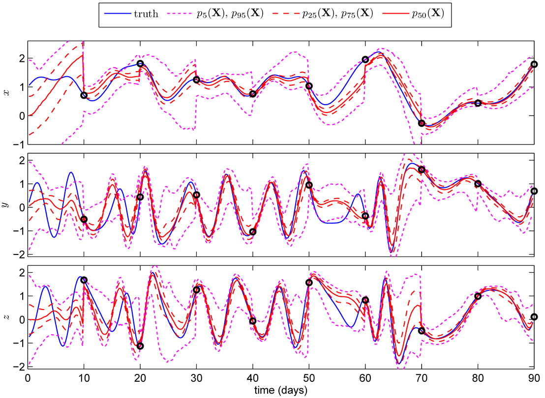
The first example is a dynamic system considered in [21], it is the well-known Lorenz-84 chaotic model, a system of three nonlinear ordinary differential equations operating in the chaotic regime. This is an example along the description of Eq. (3) and Eq. (5) in Subsection 2.1. Remember that this was originally a model to describe the evolution of some amplitudes of a spherical harmonic expansion of variables describing world climate. As the original scaling of the variables has been kept, the time axis in Fig. 1 is in days. Every ten days a noisy measurement is performed and the state description is updated. In between the state description evolves according to the chaotic dynamic of the system. One may observe from Fig. 1 how the uncertainty—the width of the distribution as given by the quantile lines—shrinks every time a measurement is performed, and then increases again due to the chaotic and hence noisy dynamics. Of course, we did not really measure world climate, but rather simulated the “truth” as well, i.e. a virtual experiment, like the others to follow. More details may be found in [21] and the references therein. All computations are performed in a functional approximation with polynomial chaos expansions as alluded to in Subsection 7.2, and the filter is linear according to Eq. (42).
To introduce the nonlinear filter as sketched in Section 6, where for the nonlinear filter the functions in Eq. (46) included polynomials up to quadratic terms, one may look shortly at a very simplified example, identifying a value, where only the third power of the value plus a Gaussian error RV is observed. All updates follow Eq. (28), but the update map is computed with different accuracy.
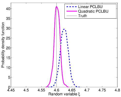
Shown are the pdfs produced by the linear filter according to Eq. (42) — Linear polynomial chaos Bayesian update (Linear PCBU) — a special form of Eq. (28), and using polynomials up to order two, the quadratic polynomial chaos Bayesian update (QPCBU). One may observe that due to the nonlinear observation, the differences between the linear filters and the quadratic one are already significant, the QPCBU yielding a better update.
We go back to the example shown in Fig. 1, but now consider only for one step a nonlinear filter like in Fig. 2, see [18].
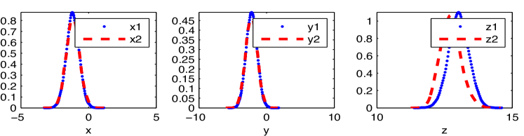
As a first set of experiments we take the measurement operator to be linear in the state variable to be identified, i.e. we can observe the whole state directly. At the moment we consider updates after each day—whereas in Fig. 1 the updates were performed every 10 days. The update is done once with the linear Bayesian update (LBU), and again with a quadratic nonlinear BU (QBU). The results for the posterior pdfs are given in Fig. 3, where the linear update is dotted in blue and labelled , and the full red line is the quadratic QBU labelled ; there is hardly any difference between the two except for the -component of the state, most probably indicating that the LBU is already very accurate.
Now the same experiment, but the measurement operator is cubic:
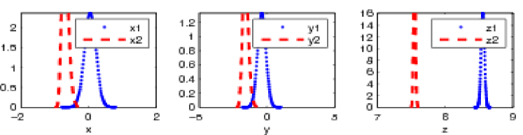
These differences in posterior pdfs after one update may be gleaned from Fig. 4, and they are indeed larger than in the linear case Fig. 3, due to the strongly nonlinear measurement operator, showing that the QBU may provide much more accurate tracking of the state, especially for non-linear observation operators.
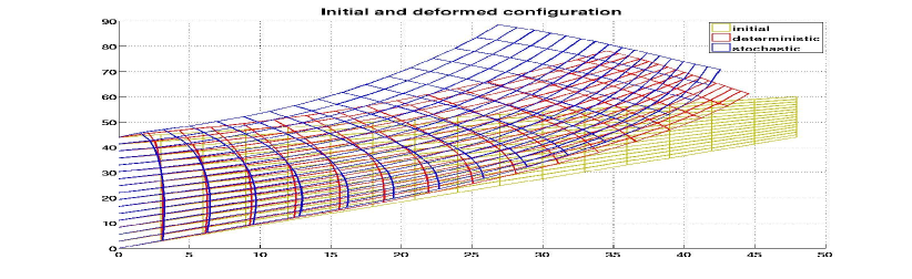
As a last example we follow [18] and take a strongly nonlinear and also non-smooth situation, namely elasto-plasticity with linear hardening and large deformations and a Kirchhoff-St. Venant elastic material law [24], [25]. This example is known as Cook’s membrane, and is shown in Fig. 6 with the undeformed mesh (initial), the deformed one obtained by computing with average values of the elasticity and plasticity material constants (deterministic), and finally the average result from a stochastic forward calculation of the probabilistic model (stochastic), which is described by a variational inequality [25].
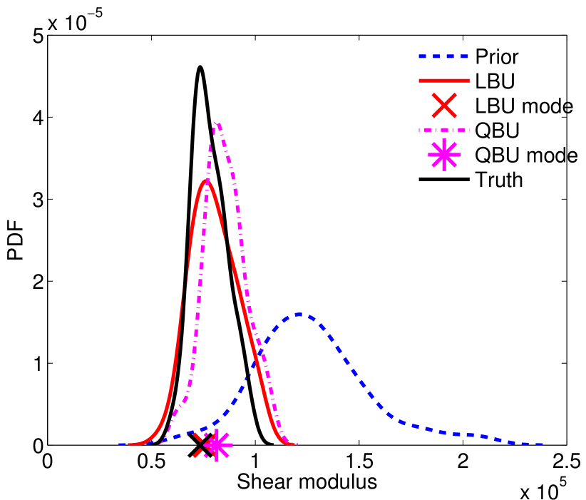
The shear modulus , a random field and not a deterministic value in this case, has to be identified, which is made more difficult by the non-smooth non-linearity. In Fig. 6 one may see the ‘true’ distribution at one point in the domain in an unbroken black line, with the mode — the maximum of the pdf — marked by a black cross on the abscissa, whereas the prior is shown in a dotted blue line. The pdf of the LBU is shown in an unbroken red line, with its mode marked by a red cross, and the pdf of the QBU is shown in a broken purple line with its mode marked by an asterisk. Again we see a difference between the LBU and the QBU. But here a curious thing happens; the mode of the LBU-posterior is actually closer to the mode of the ‘truth’ than the mode of the QBU-posterior. This means that somehow the QBU takes the prior more into account than the LBU, which is a kind of overshooting which has been observed at other occasions. On the other hand the pdf of the QBU is narrower — has less uncertainty — than the pdf of the LBU.
9 Conclusion
A general approach for state and parameter estimation has been presented in a Bayesian framework. The Bayesian approach is based here on the conditional expectation (CE) operator, and different approximations were discussed, where the linear approximation leads to a generalisation of the well-known Kalman filter (KF), and is here termed the Gauss-Markov-Kalman filter (GMKF), as it is based on the classical Gauss-Markov theorem. Based on the CE operator, various approximations to construct a RV with the proper posterior distribution were shown, where just correcting for the mean is certainly the simplest type of filter, and also the basis of the GMKF.
Actual numerical computations typically require a discretisation of both the spatial variables — something which is practically independent of the considerations here — and the stochastic variables. Classical are sampling methods, but here the use of spectral resp. functional approximations is alluded to, and all computations in the examples shown are carried out with functional approximations.
References
- [1] A. Bobrowski, Functional analysis for probability and stochastic processes, Cambridge University Press, Cambridge, 2005.
- [2] D. Bosq, Linear processes in function spaces. theory and applications., Lecture Notes in Statistics, vol. 149, Springer, Berlin, 2000, contains definition of strong or -orthogonality for vector valued random variables.
- [3] H. W. Engl and C. W. Groetsch, Inverse and ill-posed problems, Academic Press, New York, NY, 1987.
- [4] H. W. Engl, M. Hanke, and A. Neubauer, Regularization of inverse problems, Kluwer, Dordrecht, 2000.
- [5] G. Evensen, Data assimilation — the ensemble Kalman filter, Springer, Berlin, 2009.
- [6] M. Goldstein and D. Wooff, Bayes linear statistics—theory and methods, Wiley Series in Probability and Statistics, John Wiley & Sons, Chichester, 2007.
- [7] M. S. Grewal and A. P. Andrews, Kalman filtering: theory and practice using MATLAB, John Wiley & Sons, Chichester, 2008.
- [8] W. Hackbusch, Tensor spaces and numerical tensor calculus, Springer, Berlin, 2012.
- [9] W. K. Hastings, Monte Carlo sampling methods using Markov chains and their applications, Biometrika 57 (1970), no. 1, 97–109, doi:10.1093/biomet/57.1.97.
- [10] E. T. Jaynes, Probability theory, the logic of science, Cambridge University Press, Cambridge, 2003.
- [11] R. E. Kálmán, A new approach to linear filtering and prediction problems, Transactions of the ASME—J. of Basic Engineering (Series D) 82 (1960), 35–45.
- [12] D. T. B. Kelly, K. J. H. Law, and A. M. Stuart, Well-posedness and accuracy of the ensemble Kalman filter in discrete and continuous time, Nonlinearity 27 (2014), 2579–2603, doi:10.1088/0951-7715/27/10/2579.
- [13] M. C. Kennedy and A. O’Hagan, Bayesian calibration of computer models, J. Royal Statist., Series B (2001), no. 63(3), 425–464.
- [14] O. P. Le Maître and O. M. Knio, Spectral methods for uncertainty quantification, Scientific Computation, Springer, Berlin, 2010, doi:10.1007/978-90-481-3520-2. MR 2605529
- [15] D. G. Luenberger, Optimization by vector space methods, John Wiley & Sons, Chichester, 1969.
- [16] Y. M. Marzouk, H. N. Najm, and L. A. Rahn, Stochastic spectral methods for efficient Bayesian solution of inverse problems, Journal of Computational Physics 224 (2007), no. 2, 560–586, doi:10.1016/j.jcp.2006.10.010.
- [17] H. G. Matthies, Uncertainty quantification with stochastic finite elements, Encyclopaedia of Computational Mechanics (E. Stein, R. de Borst, and T. J. R. Hughes, eds.), John Wiley & Sons, Chichester, 2007, doi:10.1002/0470091355.ecm071.
- [18] H. G. Matthies, E. Zander, B. V. Rosić, A. Litvinenko, and O. Pajonk, Inverse problems in a Bayesian setting, arXiv: 1511.00524 [math.PR], 2015, Available from: http://arxiv.org/abs/1511.00524.
- [19] S. B. McGrayne, The theory that would not die, Yale University Press, New Haven, 2011.
- [20] T. A. Moselhy and Y. M. Marzouk, Bayesian inference with optimal maps, Journal of Computational Physics 231 (2012), 7815–7850, doi:10.1016/j.jcp.2012.07.022.
- [21] O. Pajonk, B. V. Rosić, A. Litvinenko, and H. G. Matthies, A deterministic filter for non-Gaussian Bayesian estimation — applications to dynamical system estimation with noisy measurements, Physica D 241 (2012), 775–788, doi:10.1016/j.physd.2012.01.001.
- [22] A. Papoulis, Probability, random variables, and stochastic processes, third ed., McGraw-Hill Series in Electrical Engineering, McGraw-Hill, New York, 1991.
- [23] M. M. Rao, Conditional measures and applications, CRC Press, Boca Raton, FL, 2005.
- [24] B. V. Rosić, A. Kučerová, J. Sýkora, O. Pajonk, A. Litvinenko, and H. G. Matthies, Parameter identification in a probabilistic setting, Engineering Structures 50 (2013), 179–196, doi:10.1016/j.engstruct.2012.12.029.
- [25] B. V. Rosić and H. G. Matthies, Identification of properties of stochastic elastoplastic systems, Computational Methods in Stochastic Dynamics (Berlin) (M. Papadrakakis, G. Stefanou, and V. Papadopoulos, eds.), Computational Methods in Applied Sciences, vol. 26, Springer, 2013, pp. 237–253, doi:10.1007/978-94-007-5134-7\_14.
- [26] A. M. Stuart, Inverse problems: A Bayesian perspective, Acta Numerica 19 (2010), 451–559, doi:10.1017/S0962492910000061.
- [27] A. Tarantola, Inverse problem theory and methods for model parameter estimation, SIAM, Philadelphia, PA, 2004.
- [28] A. N. Tikhonov, A. V. Goncharsky, V. V. Stepanov, and A. G. Yagola, Numerical methods for the solution of ill-posed problems, Springer, Berlin, 1995.
- [29] A. N. Tikhonov and V. Y. Arsenin, Solutions of ill-posed problems, John Wiley & Sons, Chichester, 1977.
- [30] D. Xiu, Numerical methods for stochastic computations: a spectral method approach, Princeton University Press, Princeton, NJ, 2010.