LOFAR/H-ATLAS: A deep low-frequency survey of the Herschel-ATLAS North Galactic Pole field

Abstract

We present LOFAR High-Band Array (HBA) observations of the Herschel-ATLAS North Galactic Pole survey area. The survey we have carried out, consisting of four pointings covering around 142 square degrees of sky in the frequency range 126–173 MHz, does not provide uniform noise coverage but otherwise is representative of the quality of data to be expected in the planned LOFAR wide-area surveys, and has been reduced using recently developed ‘facet calibration’ methods at a resolution approaching the full resolution of the datasets ($\sim 10\times 6$ arcsec) and an rms off-source noise that ranges from 100 $\mu$Jy beam^-1 in the centre of the best fields to around 2 mJy beam^-1 at the furthest extent of our imaging. We describe the imaging, cataloguing and source identification processes, and present some initial science results based on a 5-$\sigma$ source catalogue. These include (i) an initial look at the radio/far-infrared correlation at 150 MHz, showing that many Herschel sources are not yet detected by LOFAR; (ii) number counts at 150 MHz, including, for the first time, observational constraints on the numbers of star-forming galaxies; (iii) the 150-MHz luminosity functions for active and star-forming galaxies, which agree well with determinations at higher frequencies at low redshift, and show strong redshift evolution of the star-forming population; and (iv) some discussion of the implications of our observations for studies of radio galaxy life cycles.

1 Introduction

Low-frequency continuum radio emission from galaxies originates in the synchrotron process, with the two sources of energy for the required high-energy electrons and positrons being supernovae and their remnants (in star-forming galaxies) or the activity of radio-loud active galactic nuclei, which drive relativistic jets of magnetized plasma into the external medium. In principle, both of these processes provide us with information that cannot be accessed in any other way. The inferred cosmic-ray population of star-forming galaxies stores some fraction of the energy deposited by supernova and supernova remnant activity, albeit with an integration timescale that depends on radiative losses and transport processes in the host galaxy, and thus depends on the time-integrated star-formation rate, giving rise to the well-known radio/far-infrared correlation (van der Kruit, 1971; de Jong et al., 1985; Helou et al., 1985; Yun et al., 2001; Ibar et al., 2008; Murphy, 2009; Jarvis et al., 2010; Ivison et al., 2010a, b; Lacki et al., 2010; Smith et al., 2014). The luminosity and other properties (structure, spectrum, and polarization) of radio emission from radio-loud AGN offer us the only method, in the absence of deep X-ray observations for every target, of assessing the kinetic luminosity produced by the AGN, or jet power, and the radio luminosity alone is widely used for this purpose (Willott et al., 1999) although there are serious uncertainties in applying this method to individual objects (Hardcastle & Krause, 2013). In the local Universe, there is a large population of radio-loud AGN which exhibit no signatures of conventional thin-disc accretion, generally referred to as low-excitation radio galaxies or jet-mode objects (Hardcastle et al., 2007, 2009): radio observations represent the only way to study the accretion onto the central supermassive black hole in these objects and by far the most efficient way (in the absence of sensitive X-ray observations for large samples) to constrain their effects on the external medium, the so-called feedback process thought to be responsible for preventing massive star formation from the hot phase of the intergalactic medium (Croton et al., 2006).

Wide-area, sensitive radio surveys, in conjunction with wide-area optical photometric and spectroscopic surveys such as the Sloan Digital Sky Survey (SDSS: Eisenstein et al. 2011) provide us with the ideal way to study both these processes in a statistical way in the local Universe. Sensitive surveys are required to detect the radio emission expected from low-level star formation, which can be faint; star-forming objects start to dominate the radio-emitting population at luminosities below about $10^{23}$ W Hz^-1 at 1.4 GHz (Mauch & Sadler, 2007), corresponding to 4 mJy for a source redshift of 0.1 and 0.3 mJy at $z=0.3$. Wide-area surveys are required in order to find statistically meaningful samples of powerful AGN that are close enough to be optically identified and have their redshifts determined using available optical data. A key problem, however, is distinguishing between radio emission driven by low-level star-formation activity and that powered by low-luminosity AGN (Ibar et al., 2009). In an era where radio survey capabilities are expected to become vastly more powerful, it is important to develop diagnostics that will help us to understand this problem, or at least to understand its true extent. To do this we need to calibrate the radio properties of identified radio sources against their instantaneous star-formation rates and star-formation histories obtained by other means. This motivates radio observations of wide regions of the sky with good constraints on star-formation activity.

One widely used diagnostic of star formation is the luminosity and temperature of cool dust, heated by young stars. The ability of the Herschel satellite (Pilbratt et al., 2010) to make sensitive far-infrared observations over a broad bandwidth made it exquisitely sensitive to this particular tracer of star-formation activity. The Herschel-ATLAS survey (H-ATLAS: Eales et al. 2010) carried out wide-area surveys of several large areas of the sky in northern, equatorial and southern fields using the PACS (Poglitsch et al., 2010) and SPIRE (Griffin et al., 2010) instruments (at wavelengths of 100, 160, 250, 350 and 500 $\mu$m), allowing investigations of the relationship between star formation and radio emission (Jarvis et al., 2010) and between star formation and AGN activity of various types (Serjeant et al., 2010; Hardcastle et al., 2010; Bonfield et al., 2011; Hardcastle et al., 2013; Kalfountzou et al., 2014; Gürkan et al., 2015). However, these studies have been limited by the availability of high-quality radio data, as they rely on the 1.4-GHz VLA surveys Faint Images of the Radio Sky at Twenty-cm (FIRST, Becker et al., 1995) and NRAO VLA Sky Survey (NVSS; Condon et al., 1998), and, while these surveys have proved extremely valuable, they have inherent weaknesses when it comes to studying faint star formation and distant AGN. NVSS is sensitive to all the radio emission from sources extended on scales of arcminutes, but its resolution and sensitivity are low (resolution of 45 arcsec; rms noise level $\sim 0.5$ mJy beam^-1) which means that it can only detect luminous or nearby objects, and has difficulty identifying them with optical counterparts. FIRST is higher-resolution (5 arcsec) and more sensitive ($\sim 0.15$ mJy beam^-1) but its lack of short baselines means that it resolves out extended emission on arcmin scales, often present in nearby radio-loud AGN. Constructing samples of radio-loud AGN from these surveys with reliable identifications and luminosities involves a painstaking process of combining the two VLA surveys (e.g. Best et al., 2005; Virdee et al., 2013), and good imaging of the sources is often not possible.

The Low-Frequency Array (LOFAR: van Haarlem et al. 2013) offers the opportunity to make sensitive surveys of large areas of the northern sky with high rates of optical counterpart detection because of its combination of collecting area, resolution (up to 5 arcsec with the full Dutch array) and field of view. The LOFAR Surveys Key Science Project (Röttgering et al., 2006) aims to conduct a survey (the ‘Tier 1’ High Band Array survey, hereafter referred to as ‘Tier 1’: Shimwell et al. in prep.) of the northern sky at 5-arcsec resolution to an rms noise at 150 MHz of $\sim 100$ $\mu$Jy beam^-1, which for a typical extragalactic source with spectral index $\alpha=0.7$ implies a depth 7 times greater than FIRST’s for the same angular resolution. Crucially, LOFAR has good $uv$ plane coverage on both long and short baselines, and so is able to image all but the very largest sources at high resolution without any loss of flux density, limited only by surface brightness sensitivity. Deep observations at these low frequencies are rare, and the previous best large-area survey at frequencies around those of the LOFAR High Band Array (HBA) is the TIFR GMRT Sky Survey (TGSS), full data from which were recently released (Intema et al., 2016): however, this has a best resolution around 20 arcsec, which is substantially lower than the $\sim 5$ arcsec that LOFAR can achieve, and, with an rms noise of $\sim 5$ mJy beam^-1, significantly lower sensitivity than will be achieved for the LOFAR Tier 1 survey.

AGN selection at the lowest frequencies has long been recognised to provide the most unbiased AGN samples, because the emission is dominated by unbeamed radiation from the large-scale lobes, a fact which has ensured the long-term usefulness of low-frequency-selected samples of AGN such as 3CRR, selected at 178 MHz (Laing et al., 1983) or samples derived from the 151-MHz 6C and 7C surveys (e.g. Eales, 1985; Rawlings et al., 2001; Willott et al., 2002; Cruz et al., 2006). These AGN surveys, however, have had little or no bearing on star-formation work, since the flux density limits of the surveys exclude all but a few bright nearby star-forming objects. The relationship between star formation and radio luminosity at low frequencies is essentially unexplored. LOFAR observations of Herschel-ATLAS fields therefore offer us the possibility both to accumulate large, unbiased, well-imaged, samples of radio-loud AGN and to study the radio/star-formation relation in both radio-loud and radio-quiet galaxies in the nearby Universe.

In this paper we describe an exploratory LOFAR HBA observation, of the H-ATLAS North Galactic Pole (NGP) field, a rectangular contiguous area of sky in the SDSS sky area covering $\sim 170$ square degrees around $\mathrm{RA}=13.5$ h and $\mathrm{Dec}=30^{\circ}$, and therefore well positioned in the sky for LOFAR, with a substantial overlap with the position of the Coma cluster at low $z$. Our survey prioritizes sky coverage over uniform sensitivity but achieves depth comparable to the eventual Tier 1 LOFAR survey. We describe the imaging, cataloguing and source identification process and the tests carried out on the resulting catalogues. We then present some first results on the radio/far-infrared relation observed in the fields and the properties of optically identified radio sources, together with number counts for star-forming sources at 150 MHz and a first $z=0$ 150-MHz luminosity function. A subsequent paper (Gürkan et al. in prep.) will explore the 150-MHz radio/star-formation relation derived from LOFAR and H-ATLAS data and we expect to carry out further analysis of the bright AGN population.

Throughout the paper we assume a cosmology in which $H_{0}=70$ km s^-1, $\Omega_{\rm m}=0.3$ and $\Omega_{\Lambda}=0.7$.

2 Observations

Table 1: LOFAR observations of the NGP field

Field name	RA	Dec	Start date/time	Duration (h)
Central	13h24m00s	+27d30m00s	2013-04-26 17:42:15	9.7
NW	13h00m00s	+31d52m00s	2014-04-22 18:30:30	8.0
SW	13h04m00s	+25d40m00s	2014-04-25 18:17:00	8.0
NE	13h34m00s	+32d18m00s	2014-07-15 13:28:38	8.0

The NGP field was observed in four separate pointings, chosen to maximise sky covered, with the LOFAR HBA (Table 1) as part of the Surveys Key Science project. Observations used the HBA_DUAL_INNER mode, meaning that the station beams of core and remote stations roughly matched each other and giving the widest possible field of view. The first observation, which was made early on in LOFAR operations, was of slightly longer duration ($\sim 10$ h) than the others ($\sim 8$ h). International stations were included in some of the observations in 2014 but were not used in any of our analysis, which uses only the Dutch array.

In each case, the observations of the field were preceded and followed by short, 10-minute observations of calibrator sources (3C 196 at the start of the run and 3C 295 at the end). Each observation used the full 72 MHz of bandwidth provided by the HBA on the target field, spanning the frequency range 110 to 182 MHz. As LOFAR is a software telescope, multiple beams can be formed on the sky, and the total bandwidth that can be processed by the correlator exceeds the total bandwidth available from the HBA: this allowed us to observe an additional 24 MHz spread throughout this frequency range on an in-field calibrator, the bright point source 3C 287, which lies in the SE corner of the NGP field. The original intention was to use this calibrator pointing for determination of the clock offsets between the core and remote stations, but this proved unnecessary, as we shall see below. As data with non-contiguous frequency coverage could not easily be analysed using the facet calibration method (see below) at the time of our analysis, we do not consider the 3C 287 observations further.

After observation, the data were averaged by the observatory to 4 channels per sub-band (an HBA sub-band has a bandwidth of 195.3 kHz) and a 5-second integration time. No ‘demixing’ of bright off-axis sources was carried out – this was deemed unnecessary given the sky positions of bright objects like Cyg A and Cas A – and all further processing was carried out by us using the University of Hertfordshire high-performance computing facility.

3 Data processing, imaging and cataloguing

3.1 Facet calibration

The data were processed using techniques which are described in detail by van Weeren et al. (2016) (hereafter vW16) and Williams et al. (2016) (hereafter W16), implemented by us in a way which was intended to maximise the data processing efficiency on the Hertfordshire cluster. Here we give a brief overview of the processes, highlighting steps in which our approach differs from that of vW16 and W16.

Initial flagging using rficonsole was done on each sub-band of the target and calibrator observation (we used 3C 196 as the primary calibrator for all four observations) and we then solved for per station for amplitude, phase and ‘rotation angle’ – a term that accounts for differential Faraday rotation within a sub-band, as described in section 4.3 of vW16 – on the calibrator observations using the ‘Black Board Self-Calibration’ (bbs) software (Pandey et al., 2009), making use of a high-resolution model of 3C 196 kindly supplied by V.N. Pandey. Because each sub-band was treated independently, we were able to efficiently run many of these steps in parallel. We then combined the complex gain solutions on the calibrator for each sub-band, using tools in the LoSoTo package. Bad stations or sub-bands could be identified at this point by looking for large rms values or gain outliers: when one or more stations were identified as bad, we flagged them throughout the observation and re-ran the calibration.

With all bad data removed from the calibrator observations, we then fitted the phase solutions at all frequencies with a model intended to solve for the effects of clock offsets (which introduce a phase offset which is linear in observing frequency $\nu$) and the differential total ionospheric electron content, or TEC (which introduces phase offsets which go as $\nu^{-1}$). This so-called clock-TEC separation can only be run on the calibrator observations, because of their high signal-to-noise ratio, and must be run over as broad a bandwidth as possible to maximize the effectiveness of the fitting process. The result was a set of per-station clock offset values which we transferred, along with the gain amplitudes, to the data for the target field, again for each sub-band. (The ionospheric TEC values are not transferred to the target because the ionosphere toward the target will be different, and in general variable: the clock offsets, on the other hand, are not expected to vary significantly over the observation.)

The clock-corrected sub-bands on the target field were now concatenated into ‘bands’ of ten sub-bands each: such a band has a bandwidth of just under 2 MHz. This concatenation gives sufficient signal-to-noise on the target field for per-band phase calibration. The next stage was to generate a model to allow us to calibrate the fields. To do this we phase calibrated band 20 (data at frequencies of 150-152 MHz, around the frequency range where the HBA is most sensitive) using the observatory-provided global sky model, which is based on low-resolution observations from other telescopes. We then imaged this dataset with awimager (Tasse et al., 2013) at $\sim 10$-arcsec resolution, derived a list of Gaussians from the image with pybdsm (Mohan & Rafferty, 2015) and cross-matched them with the FIRST catalogue to obtain a list of sources in the field detected by both LOFAR and FIRST, with their 151-MHz and 1.4-GHz flux densities. This catalogue, while shallow, is virtually free from artefacts because of the FIRST cross-matching and has excellent positional and structural information from FIRST; this is achieved at the price of omitting only a few bright steep-spectrum or resolved objects that are not seen in FIRST.

For each band, the data were run through rficonsole again (in order to catch low-level RFI with the improved signal-to-noise of the broader bandwidth) and then averaged by a factor 2 in time and frequency, i.e. down to a 10-s integration time and 20 channels per band. This averaging was selected for computational speed in the facet calibration process, though it produces moderate bandwidth and time-averaging smearing, increasing the apparent size of sources while preserving their total flux density, beyond 2-3 degrees from the pointing centre at the full LOFAR imaging resolution of $\sim 5$ arcsec. (In this paper we work at resolutions somewhat lower than this full resolution, around $10\times 6$ arcsec, so that smearing effects are less important, but not negligible; we would expect a drop in peak flux density by a factor 0.8 and a broadening by a factor 1.2 by 4 degrees from the pointing centre, which is more or less the largest pointing centre offset considered in this work.) The cross-matched catalogue was then used (scaling appropriately using the LOFAR/FIRST spectral index) to provide the sky model for an initial phase-only calibration for each band using bbs, dividing the thousand or so cross-matched sources in each field into about 100 discrete sky regions or patches to reduce computing time. As the objective is only to provide phase calibration good enough to start the facet calibration process, small defects in the sky model are not important and in principle should not affect the final result. Again, it was possible to apply this process to all bands in parallel.

With the initial phase-only calibration computed, we corrected the data for the effect of the element beam and array factor using bbs, and all further imaging work until the very end of the process was then carried out using apparent flux densities (i.e. no primary beam correction was carried out in the imaging). At this point we could image each band [we now used wsclean (Offringa et al., 2014) for imaging, since we no longer required the primary beam correction abilities of awimager] and subtract the detected sources in the two-stage manner (first using ‘high-resolution’ images with approximately 30 arcsec beam size, then using a lower-resolution $\sim 100$-arcsec image) described by vW16. Once each band had had the sources subtracted, and we had a per-band sky model describing the subtraction that has been done, we were in a position to start the facet calibration itself.

Table 2: Spectral windows, frequencies and LOFAR band/sub-band numbers used

Spectral	Frequency range	Band	Sub-band
window	(MHz)	numbers	numbers
1	126-134	8-11	80-119
2	134-142	12-15	120-159
3	142-150	16-19	160-169
4	150-158	20-23	200-239
5	158-166	24-27	240-279
6	166-173	28-31	280-319

Our approach to facet calibration is slightly different from that of vW16. We are interested in imaging in several separate frequency ranges (which we refer to hereafter as ‘spectral windows’), since we would like to be able to measure in-band spectral indices for detected sources. In addition, facet calibrating in different spectral windows can be done in parallel, speeding the process up considerably. Accordingly, we chose to facet calibrate with six spectral windows, each made up of four bands and thus containing about 8 MHz of bandwidth (Table 2). We intentionally did not include in this spectral range the very lowest frequencies in the data, below 126 MHz, as they have significantly worse sensitivity than the higher HBA frequencies, and also discarded frequencies above 173 MHz, which are badly affected by RFI even after flagging: thus our final images contain about 48 MHz of bandwidth out of a possible total 72 MHz, but would probably gain little in sensitivity by including the missing data.

Facets were defined using our knowledge of the bright source distribution from the ‘high-resolution’ (30 arcsec) images used for subtraction: we aimed for between 20 and 30 facets per pointing in order to sample the ionosphere as well as possible, with the number actually used being determined by the number of bright sources available. Calibration positions in the facets were defined, as described by vW16, by selecting square regions (of size less than $50\times 50$ arcmin, and normally several times smaller than that) containing sources with a total flux density normally greater than 0.4 (apparent) Jy at 150 MHz. The boundaries between each facet were set using Voronoi tessellation. Each facet was then calibrated and imaged in the manner described by vW16, runnning in parallel over all six spectral windows. In practice, we always started the run for the data at 150–158 MHz before the other five, so that problems with, for example, the definition of the facets could be ironed out using a single dataset; such problems generally showed up as a failure of phase or amplitude self-calibration, resulting in poor solutions and/or increased residuals after subtraction, and were dealt with by increasing the size of the calibration region to include more sources or changing the phase/amplitude solution intervals. The whole facet calibration process, for the six spectral windows, took between one and two weeks per field, depending on the number of facets and the number of problems encountered; typically the self-calibration, imaging and subtraction step for one facet in one spectral window took 4–5 hours on a 16-core node with 64 GB RAM and 2.2-GHz clock speed. The run time per facet was shortened by a factor $\sim 2$ with respect to earlier implementations of facet calibration by the use of wsclean both for the final facet imaging and for the ‘prediction’ of the visibilities to subtract from the un-averaged data, by blanking of the images given to pybdsm for mask generation to reduce the area that it searched for sources, and by some alterations to pybdsm to improve efficiency, particularly in using the efficient FFTW algorithm for the Fourier transforms involved in cataloguing extended sources. The use of wsclean rather than a bbs subtract meant that care was necessary with the placement of facets in the final images to avoid aliasing of sources near the field edge in the prediction step, resulting in negative ‘sources’ outside the facet after subtraction. A few negative sources generated in this way propagate through into the final images, but have no significant effect on the final science results as they are not detected by the source finding algorithms.

Once the facet calibration and imaging process was complete, the resulting images for each spectral window were mosaiced into a single large image for each field, masking each facet to ensure that only the good portion of the image was used. Previous imaging of each band with awimager was used to make images of the primary beam for each band and we divided through by these images (regridding them with montage to the scale of the facet calibration images and averaging appropriately for each spectral window) to make maps of true rather than apparent flux density. (To maximize the area covered by the survey we image further down the primary beam than was attempted by e.g. W16: primary beam corrections at the edge of the largest fields can approach a factor 5.)

3.2 Flux calibration

LOFAR flux density calibration is in practice somewhat problematic: effectively, the gain normalizations transferred from the calibrator to the source are only valid if the elevation of the source and the calibrator are the same (implying the same effective telescope beam on the sky), which can only be guaranteed for a snapshot observation and is not generally true even then. This error manifests itself (after facet calibration, which removes time-dependent effects) as a frequency-dependent error in the flux scale. Currently the only method available to ensure consistency in the flux scale and correctness of in-band spectral index is to derive correction factors as a function of frequency using flux densities from other low-frequency surveys. Data available for our field include the VLSS at 74 MHz, the TGSS, 7C and 6C surveys at 150 MHz, the WENSS survey at 327 MHz and the B2 survey at 408 MHz. Of these, we elected not to use the 150-MHz data, although catalogues were available, in order to be able to use them as comparison datasets later (see below). The VLSS covers the whole survey area and should be properly calibrated on the scale of Scaife & Heald (2012), hereafter SH (we use the VLSSr catalogue of Lane et al. 2014). The B2 survey also covers the whole survey area, and SH report that it needs no systematic correction to their flux scale; we assign errors to the flux densities based on the recipes given by Colla et al. (1973). WENSS is more problematic. Firstly, the flux density of 3C 286 in WENSS is a factor 1.23 above the SH value. SH report an overall scaling factor for WENSS of 0.90, but in order to ensure that 3C 286’s flux density is correct we scale all WENSS flux densities for NVSS objects down by a factor 0.81. Secondly, WENSS only goes down to a declination of $30^{\circ}$, leaving us with almost no coverage for the SW field. We therefore supplemented our catalogues with one derived using pybdsm from the 350-MHz WSRT survey of the Coma cluster by Brown & Rudnick (2011), having verified that these data were on the SH scale by comparison to a less sensitive VLA map at 330 MHz reduced by us from the VLA archive. We refer to this survey as WSRT-Coma in what follows.

Our corrections are based on an initial catalogue of LOFAR sources which was generated by concatenating the six beam-corrected spectral window images, convolved to the same resolution using miriad, into a single data cube and then using the spectral index mode of pybdsm to extract flux densities for each ‘channel’ of the cube. We used the stacked broad-band image without beam correction as the detection image since this should have roughly uniform noise across the field. Using the spectral index mode, rather than making independent catalogues for each image, ensures that flux densities are measured from matched apertures in each spectral window. The catalogue returned at this point is of course expected to have incorrect flux calibration, which affects both the total flux densities for each source measured from the frequency-averaged images and the individual channel flux densities.

We then filtered this catalogue to include only bright LOFAR sources ($>0.1$ Jy) and cross-matched positionally using stilts with the VLSS, B2, WENSS and WSRT-Coma catalogues, requiring that all LOFAR sources should be detected in VLSS and at least one of the three higher-frequency catalogues for further consideration. This gave us 50-70 sources per field with flux densities spanning the frequency range between 74 and a few hundred MHz, all, of course, being relatively bright and with high signal to noise in the LOFAR data: the lowest flux densities at 74 MHz were around 0.4 Jy, corresponding to around 0.2 Jy at LOFAR frequencies and 0.1 Jy by 300–400 MHz. Integrated flux densities were used in all cases. We then used Markov-Chain Monte Carlo methods, implemented in the emcee python package (Foreman-Mackey et al., 2013), to fit for the LOFAR flux correction factors for each frequency. The likelihood function was calculated from the total $\chi^{2}$ for a given selection of correction factors for power-law fits to all frequencies of the data (i.e. both the unscaled VLSS and higher-frequency data and the scaled LOFAR measurements), with the normalization and power-law index for each source being free parameters which are determined with a standard Levenberg-Marquart $\chi^{2}$ minimization. We used a Jeffreys prior for the scale factors. In the first round of this fitting we included all sources, but in the second round we removed sources that were outliers in the $\chi^{2}$ distribution before re-fitting, which eliminates any sources that might be erroneous matches or heavily affected by resolution effects or might have spectra that are intrinsically poorly fit by a power law over the band, e.g. because of spectral curvature or variability; in practice this second round generally eliminated at most around 10 per cent of sources and gave results very similar to the first round. The final flux calibration factors obtained in this way for each field are tabulated in Table 3. Nominal MCMC-derived credible intervals (errors) on these correction factors are small, $<1$ per cent in all cases; the dominant source of error is of course the real deviation from a power-law model of the sources selected as calibrators, which is hard to quantify.

Table 3: Correction factors applied per field and spectral window, and mean calibrator and target elevations

Field	Spectral window number						Mean elevation
	1	2	3	4	5	6	3C 196	Field
Central	1.02	1.08	1.17	1.29	1.42	1.52	85.3	51.6
NW	0.97	1.03	1.07	1.14	1.21	1.30	82.2	58.6
SW	0.93	1.00	1.09	1.17	1.29	1.34	82.4	53.4
NE	0.72	0.75	0.79	0.84	0.89	0.92	78.2	58.9

Once this correction had been applied to each spectral window, it was possible to cross-check the flux scale between fields by comparing sources in the overlap regions. By this method we established that the flux scale for the Central, NW and SW fields was in good agreement. The NE field appeared to have a systematic offset with respect to the others, which we attribute to the fact that the correction factor fits are strongly affected by 3C 286, which is rather poorly facet-calibrated in this field (that is, relatively large artefacts remain around the source, so that its flux density is probably poorly measured). The flux densities in the NE field were systematically high. To correct for this we scaled all correction factors in the NE field by a further factor of 0.8, determined by cross-checking the flux densities with the overlapping fields, which brings the flux scales in line across the four fields; this factor is included in the numbers presented in Table 3. We comment on the effectiveness of these corrections in allowing us to recover reliable flux densities and in-band spectral indices in the next section.

These corrections were then applied to the pre-existing images, and new combined images at an effective frequency of 150 MHz, again convolved to a matching common resolution, were made by averaging the images from the 6 spectral windows for each field. These images, for each field, are our deepest view of the data, and attain an rms noise of 100 $\mu$Jy beam^-1 in the centre of the best fields. Their resolution (Table 4) is determined by the Gaussian fit by wsclean to the $uv$ plane coverage in spectral window 1, which is slightly different for each field, and particularly different for the Central field, which was observed for a longer time but without all the long baselines available in later years. As convolving to a common resolution would reduce the resolution of all the images, we elected to retain these slightly different resolutions between fields.

We then generated source catalogues for the corrected, matched-resolution data with pybdsm in its spectral index mode in the same way as described above. pybdsm’s ability to detect sources on multiple scales and to associate several Gaussian components as single sources were enabled in this cataloguing step, and sources were only catalogued if they are detected with a peak above the local $5\sigma$ value. We also make use of pybdsm’s ability to generate a map of the rms of the four 150-MHz images, referred to as the rms map in what follows.

3.3 Image quality

In general facet calibration worked well in these fields, succeeding in its two design aims of allowing greatly improved subtraction of bright sources and of making high-fidelity imaging of the data at close to the full resolution of LOFAR tractable. The resulting images are not artefact-free, but this is a consequence of not being able to amplitude self-calibrate every bright source: artefacts manifest themselves as dynamic range limitations around bright sources (particularly those that were not in the calibration sub-region of the facet) and should have only a limited effect on the quality of the final catalogue. Where facet calibration fails, it generally does so by having poor signal to noise on the calibrator, leading to poor phase and/or amplitude solutions and, generally, no improvement in self-calibration: if these poor solutions are then applied to the data we see a facet with much higher rms noise than would be expected. As discussed above, this problem can sometimes be solved by increasing the calibration region size or the interval for phase or amplitude self-calibration, but in extreme cases the facet simply has to be abandoned: we discarded a few facets at the edges of the NE and Central fields, typically at $>3$ degrees and so substantially down the primary beam, where it was not possible to obtain good self-calibration solutions (in addition to the fact that the calibrator sources are generally fainter when they are further down the primary beam, bandwidth and time-averaging smearing also start to affect the quality of the results). Other facets with poor solutions remain in the images and give rise to high-noise regions in the rms map.

Table 4: Basic field image and catalogue properties for the combined 150-MHz images

Field	Area covered	central rms	Median rms	Image resolution	Catalogued
	(sq. deg.)	($\mu$Jy)	($\mu$Jy)	(arcsec)	sources
Central	44.5	223	782	$9.62\times 7.02$	2,473
NW	34.7	104	296	$10.01\times 5.54$	5,335
SW	36.1	111	319	$9.87\times 5.49$	5,747
NE	40.6	100	382	$11.02\times 4.68$	4,172

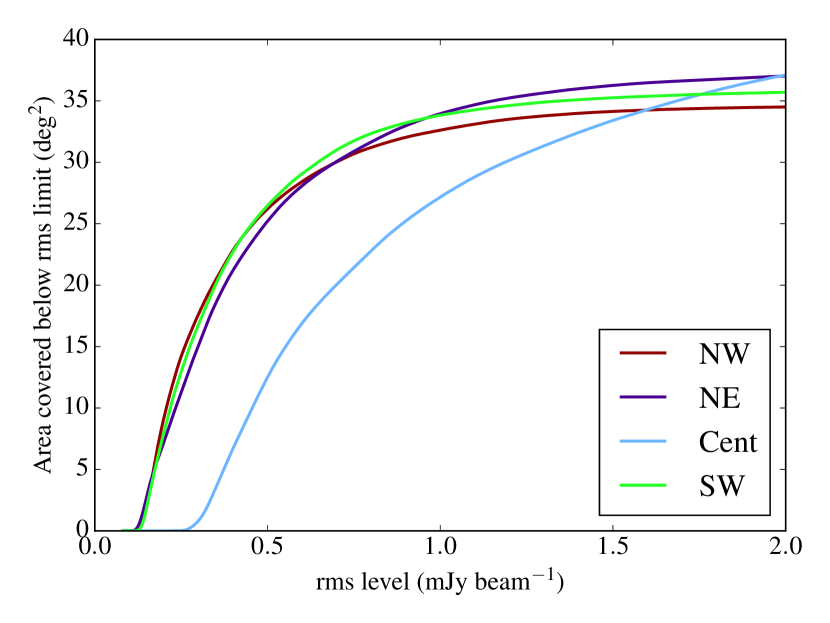
Figure 1: Cumulative histogram of the area below a given rms value, calculated from the rms noise map derived from pybdsm for the four fields. Note that, since the rms values are corrected for the telescope beam, the shape of this distribution depends on the placement of the facets as well as the intrinsic noise qualities of the image.

In Table 4 we tabulate the areal coverage, central rms, and median rms of the four fields for the broad-band 150-MHz images, along with the final resolution achieved. The median rms is the rms below which the best half of the field falls: this clearly depends on the placement of facets in the beam as well as on the image quality. The area-rms distribution of the fields is illustrated in Fig. 1. These rms values may be compared to the FIRST and NVSS rms values converted to 150 MHz for a source with $\alpha=0.75$, which are 0.8 and 2.4 mJy beam^-1 respectively. Thus, purely considering rms levels, the LOFAR survey is better than NVSS even far down the beam and always deeper than FIRST in the central 50 per cent of each field. The LOFAR data are also significantly better, in these terms, than the GMRT survey of the equatorial H-ATLAS fields (Mauch et al., 2013), which has a best rms level of 1 mJy beam^-1 at 325 MHz, corresponding to 1.8 mJy beam^-1 at 150 MHz. (We draw attention to the very different resolutions of these comparison surveys: FIRST has a resolution of 5 arcsec, NVSS 45 arcsec, and the GMRT survey between 14 and 24 arcsec. In terms of resolution, our data are most comparable to FIRST.)

The Central field, the first that was observed and the only one to be taken in Cycle 0 with the original correlator, was by far the worst of the fields in terms of noise despite its slightly longer observing duration. In this field the initial subtraction was simply not very good, suggesting large amplitude and/or phase errors in the original calibration, although it was carried out in exactly the same way as for the other fields. As a consequence, facet calibration did not perform as well as in the other fields (presumably because the residuals from poorly subtracted sources acted as additional noise in the visibilities) and there are more bad facets than in any other field, together with a higher rms noise even in the good ones. It should be noted that this is also the worst field in terms of positioning of bright sources, with 3C 286, 3C 287 and 3C 284 all a couple of degrees away from the pointing centre: we do not know whether this, the fact that the observation was carried out early on in the commissioning phase, poor ionospheric conditions, or a combination of all of these, are responsible for the poor results. The other three fields are of approximately equal quality, with rms noise values of 100 $\mu$Jy beam^-1 in the centre of the field and each providing around 31 square degrees of sky with rms noise below 0.8 mJy beam^-1 after primary beam correction. The worst of these three fields, the NE field, which has some facets where facet calibration worked poorly or not at all, was observed partly in daytime due to errors at the observatory, which we would expect would lead to poorer ionospheric quality which may contribute to the lower quality of the data.

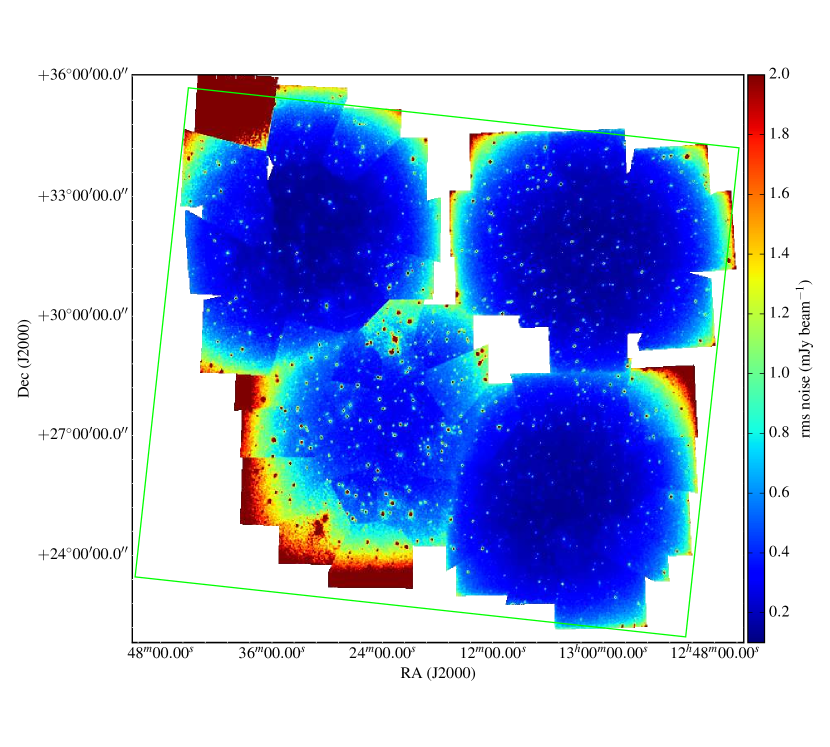
Figure 2: Map showing the sky coverage and rms values of the four fields, constructed as described in the text. Colour levels run from 100 $\mu$Jy to 2 mJy beam^-1. The green square shows the approximate boundary of the Herschel survey. The LOFAR survey is deeper (in rms terms) than FIRST, the previous most sensitive radio survey of this area, in the blue regions of the image. The many ‘point sources’ in the image are the result of dynamic range limitations around bright objects, rather than the objects themselves: the pixel size in this image is 20 arcsec, significantly larger than the image resolution.

A map of the sky coverage of the images and the rms levels, generated by resampling the full-resolution rms maps onto a grid with 20-arcsec cell size, is shown in Fig. 2. Where two fields overlap, the best rms value is shown, for reasons explained in the following section.

3.4 Catalogue generation and completeness

The final source catalogue is made by combining the four per-field catalogues. Ideally we would have combined the images of each field and done source finding on a mosaiced image, but this proved computationally intractable given the very large image cubes that result from having six spectral windows. We therefore merged the catalogues by identifying the areas of sky where there is overlap between the fields and choosing those sources which are measured from the region with the best rms values. This should ensure that there are no duplicate sources in the final catalogue. The final master catalogue contains 17,132 sources and is derived from images covering a total of 142.7 square degrees of independently imaged sky, with widely varying sensitivity as discussed above. Total HBA-band (150-MHz) flux densities of catalogued sources detected using pybdsm and a $5\sigma$ detection threshold range from a few hundred $\mu$Jy to 20 Jy, with a median of 10 mJy.

For any systematic use of the catalogue it is necessary to investigate its completeness. In the case of ideal, Gaussian noise and a catalogue containing purely point sources this could simply be inferred from the rms map, but neither of these things is true of the real catalogue. In particular, the distribution of fitted deconvolved major axes in the source catalogue shows a peak around 10 arcsec. This is probably the result of several factors, including a certain fraction of genuinely resolved sources, but we suspect that at least some of the apparent broadening of these sources is imposed by the limitations of the instrument and reduction and calibration procedure rather than being physical. Part may be due to residual bandwidth or time-averaging smearing in the individual facet images, though our lower angular resolution (relative to the similar work of W16) helps to mitigate these effects. We suspect that a significant fraction of the broadening comes from residual phase errors in the facet-calibrated images, particularly away from the calibration regions. This may be compounded in our case by the effects of combining our multiple spectral windows in the image plane – no attempt was made to align the images other than the self-calibration with an identical sky model before facet calibration, and phase offsets between the spectral windows will lead to blurring of the final image. Whatever the origin of these effects, the fact that most sources are not pointlike in the final catalogues needs to be taken into account in estimating the true sensitivity of the data.

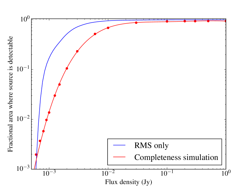
Figure 3: Completeness function for the whole survey compared with the expectations from the rms map alone. The points are the results of simulations (Poisson errors, though present, are generally smaller than symbols and are not plotted) while the smooth curve shows the best-fitting 5th-order polynomial in log space used to approximate the completeness curve and interpolate to un-simulated flux densities.

To assess this we therefore carried out completeness simulations in the standard way in the image plane [see, e.g., Heald et al. (2015) and W16] by adding in simulated sources to the residual map for each field and recovering them with pybdsm with the same settings as used for the real cataloguing. In our case, we assumed sources to be uniformly distributed at random across the whole NGP area, and placed them on the residual maps for the individual pointings based on the rms map used for cataloguing. However, rather than placing point sources (i.e. Gaussians with the parameters of the beam), we broadened the simulated sources using a Gaussian blur where the broadening $\sigma$ was itself drawn from an appropriate Gaussian distribution, chosen so as to approximately reproduce in the extracted (output) catalogues the low end of the observed distribution in deconvolved major and minor axes. The use of the residual maps also naturally takes account of artefacts around bright sources and other non-Gaussian features in the images, such as any negative holes due to wsclean aliasing effects. We ran a number of simulations for each of a range of input source flux densities, using between 10,000 and 30,000 simulated sources per run to improve the statistics. We consider a source to be matched if a source in the derived catalogue agrees with one in the input catalogue to within 7 times the nominal error in RA and Dec and 20 times the nominal error in flux density. These criteria are deliberately generous to reflect the fact that the errors on flux density and position from off-source noise are generally underestimates. Noise peaks from the residual map are removed from the catalogue before this comparison is made to avoid false positives. It is also possible to recover false detection rates in this way, but these are known to be very low (W16) and so we do not discuss them further here.

The results are shown in Fig. 3, where, for comparison, the $5\sigma$ detection level for pure point sources based on the rms map and the assumption of Gaussian noise is also shown. It can be seen that the various effects we simulate have a strong effect on completeness. The survey is complete, in the sense that a source of a given flux density can be detected essentially anywhere, only above a comparatively high flux density of $\sim 20$ mJy. At lower flux densities, the completeness curve drops more steeply than the rms map would imply. At 1 mJy, for example, the completeness curve implies a probability of detection (for a source placed at random in the field) ten times lower than would be inferred from the rms map. The curves intersect again at very low flux densities ($\sim 0.5$ mJy), but we suspect that the detection fraction here is artificially boosted by Eddington bias (i.e. simulated sources placed on noise peaks in the residual map are more likely to be recovered). The slight errors in the completeness curve resulting from this are not problematic given that there are so few sources with these flux densities in any case. Also plotted in Fig. 3 is the best-fitting 5th-order polynomial in log space fitted to the results of the simulations (taking account of the Poisson errors): this function gives an adequate approximation to and interpolation of the completeness curve, which we will make use of in later sections.

It is important to note that much of this incompleteness results from the sparse sky coverage of the observations for this project, and the poor quality of the Cycle 0 central field data. It is not representative of the expectations for the Tier 1 (wide-area) LOFAR sky survey: see W16 for a more representative completeness curve.

3.5 Association, artefact rejection and optical identification

The source catalogue was the starting point for our source association and optical identification processes, which were carried out in parallel. Optical identification was carried out using images and catalogues from SDSS Data Release 12 (Alam et al., 2015), hereafter DR12. Initially, we carried out a simple positional crossmatch for low-$z$ galaxies, selecting compact (deconvolved size $<10$ arcsec) LOFAR sources whose position matched that of an optical source from the MPA-JHU catalogue within 8 arcsec (chosen based on the distribution of offsets). This identified 1,048 LOFAR sources, of which we would expect around 30 to be chance coincidences given the number of MPA-JHU sources in the survey area. We then visually inspected the LOFAR, SDSS, FIRST and NVSS images for all the 16,084 remaining sources, initially with a single author (one of GG, MJH or SCR) inspecting each source. The person carrying out the visual inspection was asked to associate individually detected LOFAR sources, i.e. to say whether s/he believed that they were physically associated, to identify any artefacts, and, for real sources, to specify any plausible optical identification for the radio source. The NVSS images were used only to confirm the reality of faint extended LOFAR sources, which often show up well in the low-resolution NVSS data, but the FIRST images had a more important role, as they turn out often to show the flat-spectrum core of an extended LOFAR source making optical identification far more robust. Identifications by one author were cross-checked against those of another to ensure consistency and a subset (consisting of a few hundred large, bright sources) of the first pass of identifications were re-inspected visually by several authors and some (a few per cent) corrected or rejected from the final catalogue. The final outcomes of this process were (a) an associated, artefact-free catalogue of 15,292 sources, all of which we believe to be real physical objects, and (b) a catalogue of 6,227 objects with plausible, single optical identifications with SDSS sources, representing an identification fraction of just over 40 per cent. (Note that around 50 sources with more than one equally plausible optical ID are excluded from this catalogue; further observation would be required to disambiguate these sources.) This identification fraction is of interest because we can expect to achieve very similar numbers in all parts of the Tier 1 LOFAR survey where SDSS provides the optical catalogue. Forthcoming wide-area optical surveys such as Pan-STARRS1 and, in the foreseeable future, LSST (for equatorial fields), will improve on this optical ID rate.

Optical identification using shallow optical images can lead, and historically has led, to misidentifications, where a plausible foreground object is identified as the host instead of a true unseen background source. This is particularly true when the LOFAR source is large and no FIRST counterpart is seen. It is difficult to assess the level of such misidentifications in our catalogue [likelihood-ratio based methods, such as those of Sutherland & Saunders (1992), require information about where plausible optical IDs could lie in a resolved radio source that is hard to put in quantitative form] but as our resolution is relatively high, so that most sources are not large in apparent angular size and do not have more than one plausible optical ID, we expect it to be low. Sensitive high-frequency imaging over the field, and/or deeper optical observations, would be needed to make progress.

In what follows we refer to the raw, combined output from pybdsm as the ‘source catalogue’, the product of the association process as the ‘associated catalogue’ and the reduced catalogue with SDSS optical IDs as the ‘identified catalogue’. Sources in the associated or identified catalogues that are composed of more than one source in the source catalogue are referred to as ‘composite sources’ (in total 2,938 sources from the original catalogue were associated to make 1,349 composite sources). The process of association renders the pybdsm-derived peak flux densities meaningless (they are suspect in any case because of the broadening effects discussed in the previous subsection) and so in what follows unless otherwise stated the flux density of a LOFAR source is its total flux density, derived either directly from the source catalogue or by summing several associated sources.

4 Quality checks

In this section we describe the tests carried out on the catalogues to assess their suitability for further scientific analysis. From here on, except where otherwise stated, we use only the associated and identified catalogues.

4.1 Flux scale tests: 7C crossmatch

An initial check of the flux scale was carried out by crossmatching the associated catalogue with the 7C catalogue (Hales et al., 2007) over the field. Unfortunately the NGP spans the southern boundary of 7C, so we do not have complete coverage, though there is substantial overlap. The crossmatching uses the same algorithm as that described by Heald et al. (2015), i.e. we use a simple maximum likelihood crossmatch taking account of the formal positional errors in both catalogues and using the correct (Rayleigh) distribution of the offsets, but not taking into account any flux density information. Since 7C sources are very sparse on the sky, any more complicated procedure is probably unnecessary. Over the intersection of the 7C and LOFAR/NGP survey areas, there are 735 7C sources, 694 of which (94 per cent) are detected in the LOFAR images, with a mean positional offset of $\delta_{RA}=0.87\pm 0.34$ arcsec and $\delta_{\rm Dec}=0.28\pm 0.32$ arcsec. The flux limit of 7C is a few hundred mJy, so we would expect all 7C sources to be detected by LOFAR: in fact, the few nominally unmatched 7C sources are either at the edges of one of the LOFAR fields, where the sensitivity is very poor, or are actually close to a LOFAR source but with discrepant co-ordinates, which could be attributed to the very different resolutions of the surveys – 7C has a resolution of $70\times 140$ arcsec at this declination. 7C is complete above $\sim 0.4$ Jy at 150 MHz, and for sources above this flux limit the mean ratio between 7C and LOFAR 150-MHz total flux densities is $1.00\pm 0.01$, showing excellent agreement between the 7C and LOFAR flux scales, though the scatter is larger than would be expected from the nominal flux errors. We can conclude that there are no serious global flux scale errors in the catalogue, at least in the region covered by 7C (essentially the NE and NW fields).

4.2 Flux scale tests: NVSS crossmatch

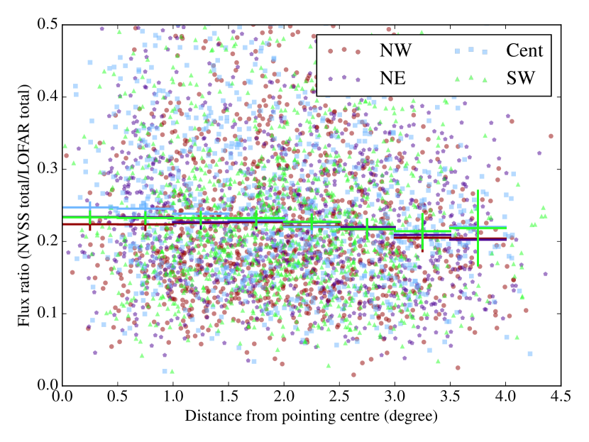
Figure 4: NVSS/LOFAR flux ratio as a function of radial distance from the pointing centre of each field. Points show individual matched sources, solid lines show the median in radial bins and its error on the approximation of Gaussian statistics.

The most suitable high-frequency survey for a direct comparison with the LOFAR results is NVSS, which is sensitive to large-scale structure, although its resolution is much lower than that of the LOFAR images. To generate a suitable catalogue we extracted the NVSS images from the image server and mosaiced them into a large image covering the whole field. We then applied pybdsm to this mosaic with exactly the same settings as were used for the LOFAR catalogue; this procedure allows us to measure accurate total flux densities for extended sources, rather than inferring them from the peak flux densities and Gaussian parametrization provided in the NVSS catalogue. Filtering our pybdsm catalogue to match the area coverage of the LOFAR survey, we found 5,989 NVSS sources. These were then crossmatched to the LOFAR data as for the 7C data, but adding a Gaussian term to the likelihood crossmatching to favour sources where the flux densities are consistent with the expected power law of $\alpha\approx 0.7$ (i.e. a term proportional to $\exp(-(S_{\rm LOFAR}-(1400/151)^{0.7}S_{\rm NVSS})^{2}/\sigma^{2})$: this helps to reduce the incidence of spurious crossmatches) and also excluding associations with a separation between NVSS and LOFAR positions of greater than 1 arcmin. We obtained 4,629 matches: that is, as expected, the vast majority of the NVSS sources have LOFAR counterparts, with a mean positional offset of $0.4\pm 0.1$ arcsec in RA and $0.05\pm 0.1$ in Dec. Counterparts are genuinely missing at the edges of the LOFAR field, where the noise is high, but we have verified by visual inspection that the comparatively large number of ‘unmatched’ sources within the field are the result of disagreements about source position (e.g. arising from structure resolved by LOFAR but unresolved by NVSS) rather than from genuinely missing sources. Similarly, most bright LOFAR sources have an NVSS counterpart. We therefore do not regard the match rate of only 77 per cent as problematic: visual inspection of the images could probably bring it close to 100 per cent.

Our expectation is that NVSS should be uniformly calibrated (VLA flux calibration uncertainties are 2-3 per cent, which should not introduce much scatter into this comparison), so the flux ratios between NVSS and the LOFAR catalogue allow an accurate check of the flux scale, subject only to the possibility that the fields have genuinely intrinsically different spectral index distributions, which could happen, for example, if the SW field were affected by the presence of the Coma cluster. For a further check of the flux scale and also its dependence on radius we computed the median NVSS/LOFAR flux ratio for all matched sources (median rather than mean to avoid effects from strong outliers which might arise from misidentifications or extreme intrinsic spectral indices) and also its dependence on distance from the pointing centre for each facet in bins of 0.5 degree in radius. We see (Fig. 4) that there are no significant flux scale (or, equivalently, spectral index) offsets between fields. The scatter is large, but much of this is imposed by the known dispersion in spectral index (see below, Section 4.6).

An encouraging result from the radial plot is that there is also no significant systematic difference with radius, within the uncertainties imposed by the scatter in the data. This suggests (a) that the primary beam correction applied is adequate, and (b) that bandwidth and time-averaging smearing at the edge of the field, beyond 2-3 degrees, do not seem to be having any detectable effect on the LOFAR total flux densities. The same comparison was also carried out using the peak flux densities of the LOFAR images and those of the cross-matched FIRST sources (see below), which should be more sensitive to smearing effects, again with no discernible radial dependence of the ratios.

4.3 Flux scale tests: TGSS crossmatch

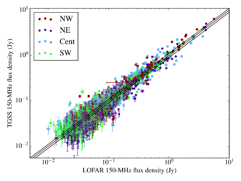
Figure 5: TGSS against LOFAR flux densities, colour-coded by field. Error bars are plotted for all data points, but in many cases are smaller than the symbols. The central line shows the median ratio between the flux densities (1.08) and the dispersion that would be implied by 10 per cent calibration uncertainties on top of this. The per-field flux scale offsets between LOFAR and TGSS data can be seen as colour gradients across the plot.

For comparison with a deeper survey than 7C at 151 MHz we make use of the data from the TGSS survey made with the GMRT with a resolution of $25\times 25$ arcsec (Intema et al., 2016). As with the NVSS data, we made a single large mosaic of the images, extracted flux densities using pybdsm, and then cross-matched positionally with the LOFAR data. There are 2896 TGSS sources in the LOFAR field, of which almost all (2449) can be cross-matched with LOFAR data. Surprisingly, given the good agreement between LOFAR and NVSS flux scales (Section 4.2), we see non-negligible per-field differences in the mean LOFAR and TGSS flux densities. There is no overall flux scale offset (as measured from median ratios of all matched sources), but the median TGSS/LOFAR ratios for the individual fields vary between 0.86 and 1.10. GMRT flux calibration is itself not reliable to better than about 10 per cent, and the overall medians will be dominated by the sources close to the centre of each field, so it is perfectly possible that much of this scatter comes from GMRT calibration uncertainties. In addition, the GMRT’s flux scale can be adversely affected by bright sources in the field, and this is apparent, for example, in the flux for the calibrator source 3C 286, which is significantly offset in the GMRT catalogue from the reference 150-MHz value of SH. We therefore do not attempt to use the TGSS images to derive further corrections to the per-field flux scale, but simply report the TGSS comparison here for the benefit of future workers. Plotting the LOFAR (corrected) total flux densities against TGSS flux densities (we restrict the comparison to sources that should be unresolved to TGSS) shows a good correlation, but, as with 7C, the scatter is larger than would be expected from the nominal errors (Fig. 5), indicating some residual calibration errors in either or both of the TGSS and LOFAR datasets. In the absence of a detailed study of the TGSS flux calibration, we cannot establish whether one or both of the datasets are responsible for this.

4.4 Positional accuracy tests: FIRST crossmatch

The 7C crossmatch shows that there are no gross astrometric errors in the catalogue, but to investigate positional accuracy in more detail we need a larger sample with higher resolution. For this purpose we cross-matched the source catalogue with the FIRST survey data in the field. There are 9,856 FIRST sources in the survey area, after filtering out sources with FIRST sidelobe probability (i.e. probability of being an artefact) $>0.05$. We restricted the crossmatching to compact LOFAR sources (fitted size less than 15 arcsec) with well-determined positions (nominal positional error less than 5 arcsec). 3,319 LOFAR/FIRST matches were obtained by this method, with a mean offset over the whole field of $\delta_{\rm RA}=0.16\pm 0.01$ arcsec and $\delta_{\rm DEC}=0.01\pm 0.01$ arcsec. Using these matches, we can determine the mean LOFAR/FIRST offset within each facet, shown in Fig. 6. Some facets have relatively few matches, so the results should be treated with caution, but a couple of points are fairly clear. Firstly, the typical offsets are small, a couple of arcsec at most: given that any offsets are likely introduced by the phase self-calibration in the facet calibration process, we would not expect them to be much larger than the pixel size of 1.5 arcsec, as is observed. Secondly, fields in which we had worse results with facet calibration also show larger offsets; by far the largest offsets are seen in some facets of the Central field, which, as discussed above, also has significantly higher noise. This is consistent with the idea that the quality of the initial direction-independent phase calibration has a strong effect on the final facet calibration results: if the initial phase calibration is poor, we expect offsets in the initial images for the first (phase-only) facet self-calibration step, and we will never be able to recover from these completely without an external reference source.

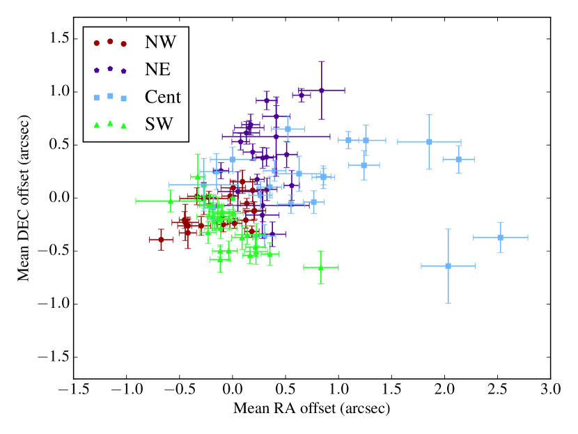
Figure 6: FIRST/LOFAR offsets in the field. The mean offset for each facet is plotted individually. Error bars show the nominal errors on the mean offsets.

4.5 In-band spectral index

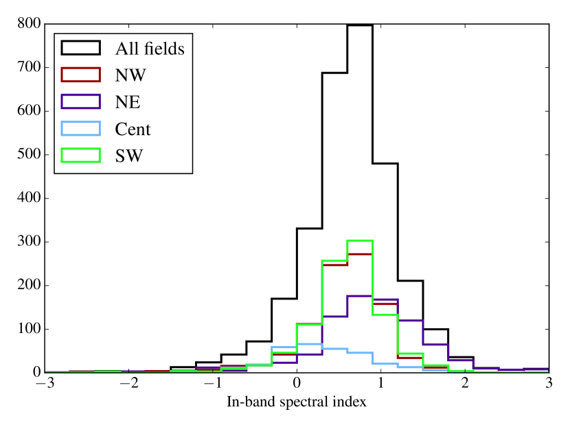
Figure 7: In-band spectral index determined from LOFAR data. The overall histogram is shown together with the histograms for each field.

We fitted power laws in frequency to the total flux densities for each source in the associated catalogue. The in-band spectral index is a sensitive test of the validity of the correction factors applied to the flux densities in each field prior to combination, as even small calibration errors will lead to large biases in in-band spectral index over the relatively narrow HBA band alone. Many sources have poor $\chi^{2}$ values (suggesting that the errors in the catalogue are underestimated) or large errors on the spectral index (estimated from the fitting covariance matrix). The in-band spectral index distribution for the overall associated catalogue and the four fields is shown in Fig. 7, where we plot only sources with nominal $1\sigma$ spectral index errors of $<0.2$ and exclude the highest $\chi^{2}$ values ($\chi^{2}>80$). It can be seen that, although the overall in-band spectral index distribution is reasonable and peaked around the expected value (0.6–0.7), the catalogues for the four fields have rather different distributions. The central field, in particular, shows a peak at flat spectral index values which must be the result of the generally poorer quality of the data in this field, while the NE field has an excess of steep-spectrum sources. By contrast, the normalization of the power-law fits at 150 MHz is generally in good agreement with the broad-band total flux density we measure. We conclude that in-band spectral indices cannot be reliably compared between fields in this dataset, though sources with extreme apparent in-band spectral index remain interesting topics for further investigation. Reliable absolute in-band spectral index measurements will require the LOFAR gain transfer problems to be solved by the use of a correctly normalized beam model.

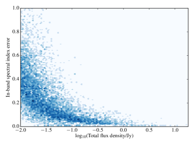
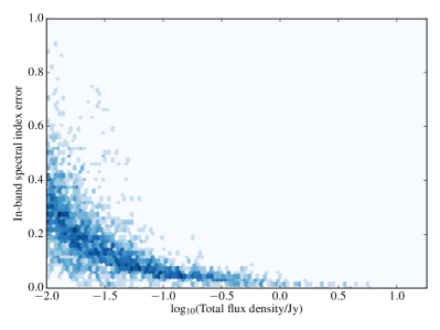
Figure 8: Density plot of errors on the in-band spectral index as a function of total LOFAR flux density. Left: all sources and fields. Right: only the central 2 degrees of the NW, NE and SW fields are plotted.

We can in addition comment on the errors on the in-band spectral index to be expected from HBA data. Fig. 8 shows the error on in-band spectral index as a function of flux density for the associated catalogue, both for the whole catalogue and for the inner 2 degrees of the three best fields, which should be more representative of Tier 1 quality. It can be seen that errors are typically less than $\pm 0.1$ only for bright sources, with flux densities $>100$ mJy, even in the centres of the best fields. For almost all sources, therefore, a much cleaner spectral index determination will be obtained by comparing with NVSS, which will detect all but the steepest-spectrum LOFAR sources with LOFAR flux densities above a few tens of mJy. It will be possible to use in-band spectral index to select sources which are extremely steep-spectrum (and so undetected in NVSS) but this will only be reliable, even after LOFAR gain calibration problems are solved, if they are also bright.

4.6 Out-of-band spectral index

We use the NVSS/LOFAR crossmatch described above (Section 4.2) to construct a distribution of spectral indices between 150 MHz and 1.4 GHz (Fig. 9). The median NVSS/LOFAR spectral index is 0.63, with almost no differences seen between fields. It is important to note that the effective flux density limit of $\sim 2.5$ mJy for point sources in the NVSS data biases the global spectral index distribution to low (flat) values – only flat-spectrum counterparts can be found to faint LOFAR sources (Fig. 9). If we restrict ourselves to sources where this bias is not significant, with LOFAR flux densities above $\sim 30$ mJy, the median spectral index becomes $0.755\pm 0.005$ (errors from bootstrap), in good agreement with other determinations of the spectral index distribution around these frequencies (e.g., Mauch et al., 2013, and references therein). Deeper 1.4-GHz data with comparable $uv$ plane coverage to LOFAR’s are required to investigate the spectral index distribution of faint sources.

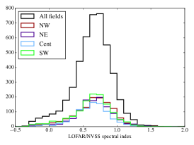
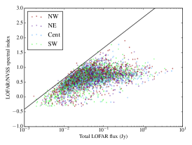
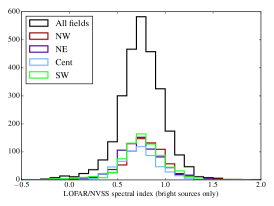
Figure 9: Left: histogram of LOFAR/NVSS spectral indices for all sources and for the individual fields. Centre: the relationship between spectral index and flux density: the solid line shows the region to the top left that cannot be populated by point sources given the NVSS sensitivity limit. Right: the histogram of spectral index for bright ($S_{150}>30$ mJy) sources only.

With both the in-band and LOFAR/NVSS spectral indices in hand, we can compare the two, and this comparison is shown in Fig. 10. Here we plot the $\sim 2,000$ sources that have LOFAR flux density $>30$ mJy and also satisfy the requirement that the nominal error on the in-band spectral index is $<0.1$ and the fit is acceptable. A general tendency for the in-band spectral index to be flatter than the LOFAR/NVSS index is observed, unsurprisingly, but many sources exhibit unrealistically steep (in the NE field) or flat (in the Central field) in-band indices, and in general the scatter in the plot is probably dominated by the known per-field biases in in-band index. It is possible to identify in this plot some individual sources that plausibly have interestingly steep, inverted or curved spectra, but the unreliability of the in-band index limits its use.

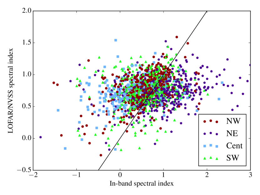
Figure 10: The in-band and NVSS/LOFAR spectral indices compared. The solid line shows equality between the two spectral indices. In general increasing spectral steepness with frequency means that we would expect points to lie above this line.

4.7 The optical identifications

As noted above, 6,227, or approximately 40 per cent, of the sources in the associated catalogue have optical identifications with either galaxies or point-like objects (presumably quasars) from the SDSS DR12 photoobj table. Of these, 1,934 have spectroscopic redshifts in the specobj table and an additional 3,660 have photometric (but not spectroscopic) redshifts, leaving 633 with no redshift information (we discard objects with nominal errors $>0.3$ on the photometric redshift). 263 objects are classed as pointlike in the photometry catalogue based on the prob_psf field, of which 89 have spectroscopic redshifts; the pointlike objects with spectroscopic redshifts are likely almost all quasars and we refer to them as quasars in what follows.

The highest spectroscopic redshift in the sample is for a quasar at $z=5.2$, but no object that is not a quasar has a redshift much greater than 1, as expected given the magnitude limits of SDSS; the sharp cutoff in photometric redshifts at $z\approx 1$ is presumably a consequence of the absence of $z>1$ objects from the training sets used in SDSS photo-$z$ determination (Beck et al., 2016), but the locus of magnitudes of radio-galaxy hosts with spectroscopic redshifts clearly intercepts the SDSS $r$-band magnitude limit of 22.2 at this redshift in any case. Detecting higher-redshift radio galaxies will require deeper optical data. The spectroscopic coverage of the galaxies that we do detect is excellent due to the presence of spectra from the Baryon Oscillation Spectroscopic Survey (BOSS: Dawson et al. 2013) in DR12, and as a result the number of objects with spectroscopic redshifts is comparable to that in the FIRST/Galaxy and Mass Assembly (GAMA: Driver et al. 2009, 2011)-based sample of Hardcastle et al. (2013), although the distribution of redshifts is rather different. The WEAVE-LOFAR project (Smith, 2015) aims to obtain spectra and redshifts for essentially all of the radio sources in the field.

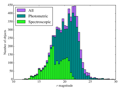
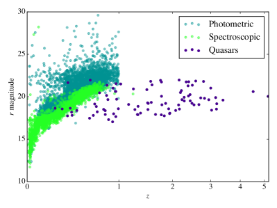
Figure 11: Left: the distribution of identified sources with spectroscopic, photometric, and no redshifts as a function of $r$-band magnitude. The second peak of spectroscopic redshifts at $r\approx 20$ is due to BOSS selection. Right: $r$-band magnitude as a function of redshift. Redshift is plotted on a $\log(1+z)$ scale but labelled with $z$ values.

In Fig. 11 we plot the Petrosian $r$ magnitude from SDSS for the optically identified sample, showing objects with spectroscopic, photometric or no redshift. We see that the sample is virtually spectroscopically complete at $r<17.7$ mag, and almost all sources have a spectroscopic or photometric redshift at $r<19$ mag. A clear lower limit in magnitude at a given redshift is seen, expected since radio-loud AGN tend to be the most massive galaxies at any redshift; the very few sources with an apparent magnitude too bright for their redshift are likely to be due to erroneously high photometric redshifts, but these are too small in number to significantly affect our analyis. We also note a small population of objects that are very faint in $r$, due presumably to SDSS photometric errors in the $r$-band – most of these objects have more reasonable magnitudes in other SDSS bands.

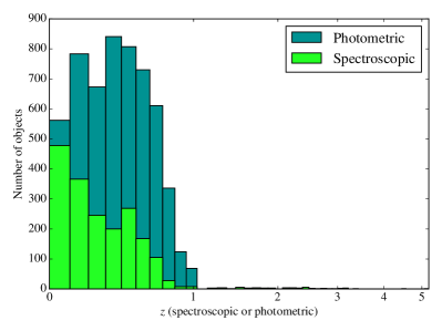
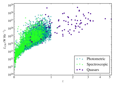
Figure 12: Left: redshift and right: radio luminosity distributions for the optically identified galaxy catalogue and the subsample with spectroscopic redshifts. Redshift is plotted on a $\log(1+z)$ scale but labelled with $z$ values.

Fig. 12 shows the distribution of spectroscopic and photometric redshifts in the galaxy sample, and the corresponding radio luminosities (where we use a single spectral index of $\alpha=0.7$ for K-correction). We see that the radio luminosities of the optically identified sample span the range from $10^{21}$ W Hz^-1 (where we would expect star formation to be the dominant process) through to well above $10^{26}$ W Hz^-1 (the nominal FRI/FRII break luminosity at 150 MHz) even for the spectroscopic subsample. The wide area and high sensitivity provided by LOFAR coupled with the availability of spectroscopy for a large number of faint galaxies in SDSS DR12 drives the wide range in radio luminosity that we observe.

5 Initial science results

In this section we discuss some scientific conclusions that can easily be drawn from the various catalogues that we have constructed. Detailed analyses of all these topics will be presented in later papers.

5.1 Source counts

The associated catalogue allows us to construct the standard Euclidean-normalized differential source counts plot for the LOFAR sample, and this is shown in Fig. 13. For comparison at the bright end, we plot the 6C 151-MHz source counts of Hales et al. (1988). There is excellent agreement between the normalization and slope of the 6C and LOFAR data where they overlap, given the Poisson uncertainties on numbers of sources at the bright end in the LOFAR data. Our source counts are corrected for completeness (Section 3.4) and of course take account of physical associations between objects in the original catalogue, but are not corrected for any other effects. W16, in their similar but higher-resolution study, suggest that resolution bias, i.e. the fact that resolved sources are less likely to be detected, affects the counts significantly below a few mJy, where the SNR is low, and this can be seen affecting the sub-mJy flux counts in the comparison of their results with ours in Fig. 13; more detailed completeness simulations taking into account the intrinsic distribution of source sizes would be necessary to have confidence in the source counts at the very faint end of this plot. Elsewhere our results are close to, but generally slightly above, those of W16, which may be a result of our different approach to completeness corrections.

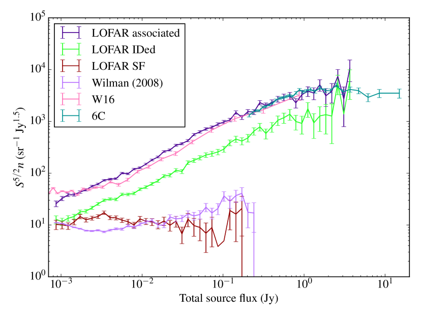
Figure 13: Euclidean-normalized differential source counts from the LOFAR associated catalogue after completeness correction. Overplotted are the 6C counts from Hales et al. (1988), the LOFAR counts from W16, the counts for the identified catalogue, and the counts for objects classed as star-forming (see Section 5.3) with the corresponding counts for SFGs from the simulations of Wilman et al. (2008). For clarity the very few points on the simulated SFG line with total flux density greater than 0.25 Jy are not plotted. Error bars are suppressed when there is only one count in the corresponding bin.

5.2 Cross-match with H-ATLAS

The H-ATLAS project produces maps and catalogues following the methods described by Pascale et al. (2011) (SPIRE mapping), Ibar et al. (2010) (PACS mapping) and Rigby et al. (2011) (cataloguing). An up-to-date description of the process for the public data, shortly to be released, will be provided by Valiante et al. (in prep.) and descriptions of the NGP maps and catalogues will be provided by Smith et al. (in prep.) and Maddox et al. (in prep.) respectively.

The currently available H-ATLAS catalogue of the NGP field contains 539,757 sources detected at approximately $2\sigma$ significance, of which 443,500 overlap with the LOFAR images. For the purposes of flux comparisons we restrict ourselves to sources with 250-$\mu$m signal-to-noise (taking account of confusion noise) $>4.0$, of which there are 94,008 in the LOFAR field; this is a similar significance level to the cut that will be applied in the forthcoming NGP data release, and implies a typical 250-$\mu$m flux density limit of around 30 mJy. Clearly only a small fraction of these Herschel sources are detected with LOFAR. We cross-matched on both LOFAR positions and the positions of optical identifications, using the same maximum-likelihood crossmatch as described above for radio catalogue matches, with a maximum permitted offset of 8 arcsec. To do this we take the error on Herschel positions to go as $1/SNR$, normalizing to a positional error of 2.4 arcsec for a SNR of 4.5 based on the results of Bourne et al. (in prep.) on the optical crossmatching to the Phase 1 H-ATLAS data release. We find 2,994 matches to LOFAR positions and 1,957 matches to optical positions — the latter being more reliable as the optical positions are better determined, but representing a smaller number of LOFAR objects as not all have optical IDs. A flux-flux plot (Fig. 14) shows the expected two branches, one where there is a good correlation between the radio and Herschel flux densities, and one where there is none, representing respectively star-forming galaxies and radio-loud AGN (some, but not all, of which will be detected in the H-ATLAS images due to their star-formation activity). The flux-flux relationship for the detected star-forming objects appears approximately linear and could be represented by $S_{\rm 250\ \mu m}\approx 20S_{\rm 150\ MHz}$, as shown on Fig. 14; such a relationship is consistent with the $z=0$ radio/far-infrared (FIR) correlation observed at 1.4 GHz for sources detected in both bands (Jarvis et al., 2010; Smith et al., 2014) where the parameter $q_{250}=\log_{10}(S_{\rm 250\ \mu m}/S_{\rm 1.4\ GHz})\approx 2.0$, assuming a spectral index of 0.7 for these objects.

The LOFAR detection fraction (Fig. 14) is low for all Herschel flux densities after the brightest ones, but certainly lower for the fainter objects, as would be expected given the flux-flux relationship and the fact that the sensitivity of the LOFAR images is not constant across the sky. It is interesting to ask whether such an explanation quantitatively predicts the detection fraction, which we can do if we assume that the flux-flux relationship estimated above holds good for all H-ATLAS sources. We can then use the LOFAR completeness curve to estimate which of the H-ATLAS sources should have been detected in the LOFAR band. In fact (Fig. 14) we would expect to detect many more sources (the simulations show this number to be around 12,000) than we actually do if $S_{\rm 150\ MHz}$ were equal to $0.05\,S_{\rm 250\ \mu m}$ for all Herschel sources. While the flux-flux correlation we see in the data must be correct for the brightest sources (we would be able to detect sources with, for example, 250-$\mu$m flux densities at the Jy level and mJy-level LOFAR flux densities, but none exist) the true flux-flux relationship for the bulk of Herschel sources needs to be at least a factor 2 below the naive estimate derived from the correlation seen for the brightest sources in order to come close to reproducing the actual detection statistics. This is again consistent with the results of Smith et al. (2014), who showed that stacking radio luminosities including sources not detected in the radio gave rise to $q_{250}$ values $\sim 2.5$. The implications here are important: even without analysing the luminosity distribution, we can see that radio/FIR relations derived from samples flux-limited in both radio and FIR are likely to be strongly biased unless non-detections are taken into account, with implications for the radio emission expected to be seen from star-forming objects in the distant Universe. Here we do not speculate whether this bias arising from the combined radio-FIR selection is due to true radio deficiency in some star-forming galaxies or to other effects such as the differing dust temperatures of objects selected at 250 $\mu$m (Smith et al., 2014). Later papers (Gürkan et al in prep.; Read et al in prep.) will discuss the relationship between radio emission and star formation in more detail.

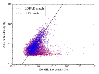
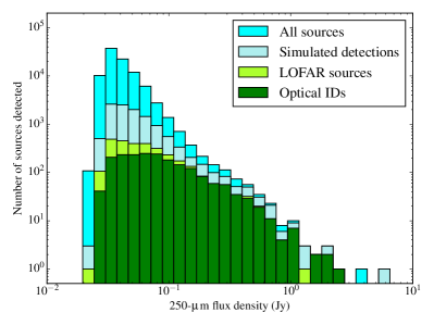
Figure 14: Results of cross-matching Herschel and LOFAR sources. Left: LOFAR/H-ATLAS flux density plot showing positional crossmatches to the LOFAR positions (red) and positions of optical counterparts (blue). Right: detection histogram, showing the distribution of 250-$\mu$m flux densities in the whole area-matched sample, the simulated number of detections if $S_{\rm 150\ MHz}$ were $0.05\,S_{\rm 250\ \mu m}$ for all sources, the distribution of flux densities of sources matched to LOFAR positions and the distribution for sources matched to SDSS sources. Note the logarithmic axes: at $S_{250}<0.1$ Jy fewer than ten per cent of the Herschel sources are detected by LOFAR.

5.3 AGN and star formation in the optically identified sample

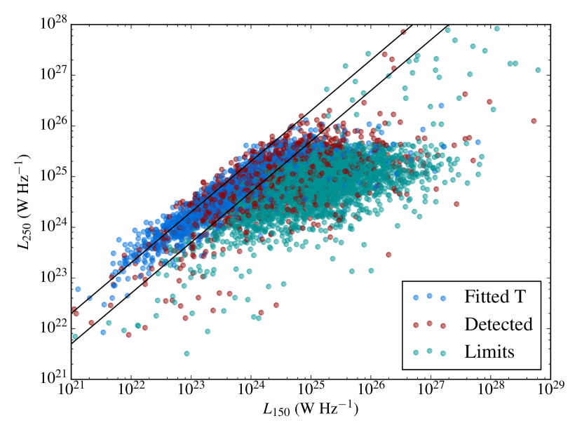
Figure 15: 250-$\mu$m far-infrared luminosity, estimated as described in the text, as a function of LOFAR radio luminosity. Objects are colour coded depending on whether they have temperature measurements, are detected at the $2\sigma$ level at 250 $\mu$m but without a valid temperature measurement, or are $2\sigma$ upper limits at 250 $\mu$m. The division into detected and non-detected sources at this level is for plotting purposes only and plays no part in the analysis. Solid lines show $q^{\prime}_{250}=20$ and $q^{\prime}_{250}=5$, where $q^{\prime}_{250}$ is as defined in the text.

We made use of the Herschel data to separate AGN and star formation in the optically identified sample. To do this we measured Herschel flux densities from all five bands directly from the H-ATLAS maps at the positions of all optical identifications with redshifts in the manner described by Hardcastle et al. (2013). We then fitted modified black-body models with $\beta=1.8$ [the best-ftting value derived by Hardcastle et al. (2013) and Smith et al. (2013)] to all objects with a $2\sigma$ detection in more than one Herschel band, accepting fits with good $\chi^{2}$ and well-constrained temperature, in the manner described by Hardcastle et al. (2013). This process gives us 1,434 dust temperatures and luminosities, with a mean dust temperature of 24.5 K. For the remaining objects, we estimate the 250-$\mu$m IR luminosity, $L_{250}$, from the 250-$\mu$m flux density alone, K-correcting using $\beta=1.8$ and $T=25$ K; we calculate a luminosity in this way for all objects, including non-detections. The temperature and $\beta$ parameters are only used here to provide a K-correction at 250 $\mu$m, rather than to calculate an integrated luminosity, and so the effects on the data should be very limited at the low redshifts of the majority of objects in our sample. The resulting radio-FIR luminosity plot is shown in Fig. 15. A clear sequence of the radio-FIR correlation can be seen, driven mostly by detected objects, as expected given the results of the previous subsection; the correlation may be slightly non-linear but at low luminosities/redshifts is broadly consistent with a constant ratio of about a factor 20 between the two luminosities. [It would not be surprising to see some non-linearity given the dependence of the radio-FIR correlation on dust temperature discussed by Smith et al. (2014): once again, we defer detailed discussion of the radio/FIR correlation to Gürkan et al. (in prep.).] Radio-loud AGN lie to the right of this correlation, i.e. they have an excess in radio emission for a given FIR luminosity. The scattering of points at high luminosities comes from the high-$z$ quasar population, where the K-corrections almost certainly break down to a large extent and where there may be some contamination of the FIR from synchrotron emission.

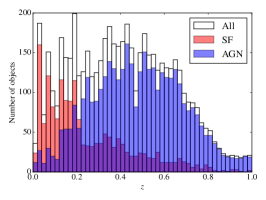
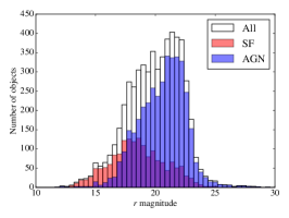
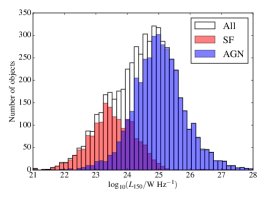
Figure 16: Distributions of key quantities for the whole sample and after AGN/star-formation separation as described in the text. In each histogram white shows the distribution of the parent sample, red star-forming objects, and blue AGN, with the overlapping regions of the two coloured histograms appearing in purple.

To make a quantitative separation between the two classes of object we define the quantity $q^{\prime}_{250}=L_{250}/L_{150}$ – we take the ratio here rather than its log, as is more conventional, to allow for the negative values of $L_{250}$ which may be assigned to Herschel non-detections. We use the value of $L_{250}$ derived from temperature fitting where available and from the 250-$\mu$m flux density otherwise. Then we take a source to be an AGN if $q^{\prime}_{250}<5$, and a star-forming object otherwise (the division being indicated by a line on Fig. 15). By this classification, 3,900 of the objects with redshifts are AGN and the remaining 1,667 are star-forming galaxies (SFGs). Consistent with expectation, these two populations have very different distributions in redshift, galaxy magnitude and 150-MHz luminosity (Fig. 16). The dividing line used here is, of course, arbitrary, though it is chosen so as to isolate the radio/FIR relation at low luminosities. We do not expect a clear separation between the two classes in $q_{250}$ since radio-loud AGN may occur in strongly star-forming galaxies. However, we checked the classification by testing what fraction of sources in the two classes are morphologically complex, using as a proxy for this multi-component sources with a maximum component separation of $>20$ arcsec (to avoid sources that are only moderately resolved by LOFAR). We find that of the 275 such sources, all but 4 are in the AGN class, and of the four extended objects classed as SFGs, 3 are genuinely extended very nearby galaxies; only one is a clear double which should be classified as an AGN, and that turns out to be one of the quasars that contaminate the high-luminosity end of Fig. 15, 14 of which have $q^{\prime}_{250}$ above the SF threshold. These objects are easily excluded from our SF catalogue and, apart from them, we do not appear to be including in the SF class any significant number of double AGN, suggesting, at least, that the SFG class is not strongly contaminated by AGN. The fraction of morphologically complex sources increases immediately below $q^{\prime}_{250}=5$, consistent with the idea that this is a useful dividing line.

The source counts of objects classed as SFGs (Fig. 13) show good agreement with the SKADS model counts of Wilman et al. (2008) in both normalization at the lowest flux densities and slope (i.e. flat when Euclidean-normalized): the only difference is that we lack the sky area to find extremely bright SFGs, and that we find slightly higher numbers of SFGs at flux densities of 2–4 mJy. This suggests that we are correctly classifying the vast majority of both SFGs and AGN. Misclassification of SFGs would lead to inconsistencies in normalization; contamination of the SFGs with AGN would lead to inconsistencies in slope. Residual differences may be due to cosmic variance – our sky area is considerably smaller than that simulated by Wilman et al. (2008). Our results contrast with those of Simpson et al. (2012) and Lindsay et al. (2014), who both found a deficit of faint objects at low $z$ at 1.4 GHz compared to the SKADS models; it is possible that this is evidence that LOFAR’s short baselines allow it to pick up a population of low-z SF sources resolved out by high-resolution VLA surveys. We note (Fig. 16) that we continue to find objects classed as SF up to the highest redshifts in our sample, and up to radio luminosities of $10^{25}$ W Hz^-1; these objects must, if correctly classified, be strongly star-forming galaxies with SFR of hundreds of solar masses per year.

We conclude that Herschel data, where available, offer a reliable and simple method of carrying out AGN/star-formation separation in LOFAR data at Tier 1 depth.

5.4 Luminosity functions

We construct the low-redshift 150-MHz luminosity function from sources with $r<19$ mag, excluding quasars. Below this limit, 1809 of our 1917 candidate identifications (95 per cent) have redshifts (1190 spectroscopic) and so we are able to construct a luminosity function without much normalization uncertainty. 1017 of the 1809 are classed as SFGs by the $q^{\prime}_{250}$ criterion, the rest are AGN. We drop at this point 2 AGN with photometric redshifts that are clear outliers on the $r$-$z$ plot (Fig. 11) leaving a sample of 1017 SFGs and 790 AGN with a maximum redshift just over $0.4$. This large redshift range means that we may be somewhat affected by cosmological evolution; the median SFG redshift is 0.12 and for AGN it is 0.24. We return to this point below. We expect that there are very few unidentified radio sources which should in fact be identified with $r<19$ galaxies, setting aside small gaps in the DR12 photometric catalogues around bright stars and the like, so that a luminosity function with these constraints should be representative of the true source population.

In order to calculate the luminosity function we must deal with the effects of K-correction in the optical. We first of all calculated absolute $g$ and $r$ magnitudes for our targets using the methods of Chilingarian et al. (2010), correcting for an average Galactic reddening using astroquery to query the IRSA Dust Extinction Service and retrieve dust extinction calculated according to Schlafly & Finkbeiner (2011). A colour-magnitude diagram constructed for the $r<19$ objects shows a good separation into red sequence and blue cloud largely dominated by AGN and star-forming objects respectively, as expected.

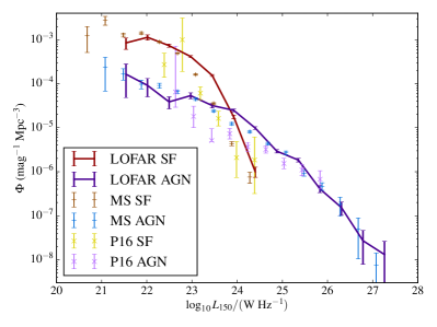
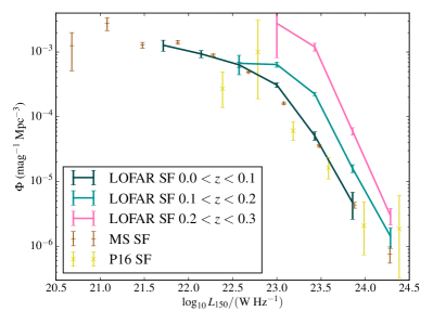
Figure 17: Left: the 150-MHz luminosity function in the H-ATLAS field dividing the sources into SFG and AGN as described in the text. Solid lines show the LOFAR-derived luminosity function: light points with error bars show the 1.4-GHz luminosity function from Mauch & Sadler (2007) and the 325-MHz luminosity function of Prescott et al. (2016), scaled assuming a constant $\alpha=0.7$. Error bars are Poissonian from number counts in bins only. Right: the same plot, but for the SFG only, dividing into three redshift bins.

We then computed the luminosity function in the standard way, i.e. by binning $1/V_{\rm max}$, where $V_{\rm max}$ is the maximum volume out to which a source can be seen given the radio and optical limits. We calculate $V_{\rm max}$ separately for optical and radio and adopt the smaller of the two. For the radio, $V_{\rm max}$ is calculated as $\int d_{\rm max}\mathrm{d}A$, where we use the completeness function described in Section 3.4 to compute the area over which sources can be seen out to a given depth. For the optical, the survey is assumed to be uniform, but we invert the approximations of Chilingarian et al. (2010) to derive K-corrections as a function of redshift and intrinsic ($M_{g}-M_{r}$) colour.

The results for the whole sample are shown in Fig. 17 (left panel). For AGN, we see overall good agreement with a scaled ($\alpha=0.7$) version of the luminosity functions of Mauch & Sadler (2007) at 1.4 GHz or Prescott et al. (2016) at 325 MHz, implying little variation in the spectral index as a function of radio luminosity. However, the luminosity function for SFG clearly has an excess with respect to the literature catalogues at higher luminosities. We attribute this to redshift evolution of the SFG population. This can clearly be seen in the right-hand panel of Fig. 17 where we plot the SFG luminosity function only, broken down into redshift bins. A strong positive luminosity function evolution with redshift is evident, and the lowest-redshift luminosity function is now in excellent agreement with that of Mauch & Sadler (2007). By contrast, we have verified that the AGN luminosity function shows no significant variation out to $z=0.4$, the limit of our magnitude-limited sample, presumably because the AGN in our sample are largely low-excitation radio galaxies which are expected to show only weak cosmological evolution (Best et al., 2014; Pracy et al., 2016). A future paper (Williams et al. 2016b) will discuss the luminosity function evolution for radio-loud AGN, both low-excitation and high-excitation using the deeper optical data in the Boötes field.

The strong radio luminosity function evolution we see for SFGs is striking. We naturally expect some evolution given the known overall evolution of the star-formation density of the universe (e.g., Madau et al., 1996; Hopkins & Beacom, 2006). In wide-area surveys hints of positive evolution have been seen for some time (Machalski & Godlowski, 2000; Condon et al., 2002). However, most work in this area has focussed on deep fields, and this has shown that the luminosity function (e.g. Haarsma et al., 2000; Smolčić et al., 2009; McAlpine et al., 2013), the specific star-formation rate estimated from the radio (e.g. Karim et al., 2011; Zwart et al., 2014) and the total radio-estimated star-formation rate density (e.g Seymour et al., 2008) all evolve positively in the redshift range $z=0$ – 1. What is unusual about our sample, other than the fact that it is calculated at 150 MHz, is that it has the area to see this evolution directly at low redshift, coupled with the ability of the H-ATLAS data to allow AGN/SF separation over such a wide area. Although the error bars are large, Fig. 17 implies that pure luminosity evolution has the form $\sim(1+z)^{5}$, which is steeper than the $\sim(1+z)^{2.5}$ found in most earlier work on the radio luminosity, suggesting either some difference in our selection or a real change in the redshift dependence at low radio luminosity and $z$. The corresponding positive evolution at low $z$ in the far-IR is relatively well known (Dye et al., 2010; Magnelli et al., 2013; Gruppioni et al., 2013) and seems to imply a similarly strong evolution with redshift (Dye et al., 2010), but, unlike the far-IR where dust mass evolution may also be implicated (Dunne et al., 2011), the radio data – if contaminating AGN can be removed – provide an unambiguous tracer of star formation evolution comparable to the ultraviolet or H$\alpha$. More optical identifications and spectroscopic redshifts for objects in the NGP field, and LOFAR observations of the equatorial H-ATLAS fields, will enable us to investigate this evolution of the low-frequency luminosity function to higher redshift in future, and to compare to the results at 1.4 GHz and to the evolution of other star formation tracers (see, e.g., Mancuso et al., 2015).

5.5 The power/linear-size diagram and the incidence of giant sources

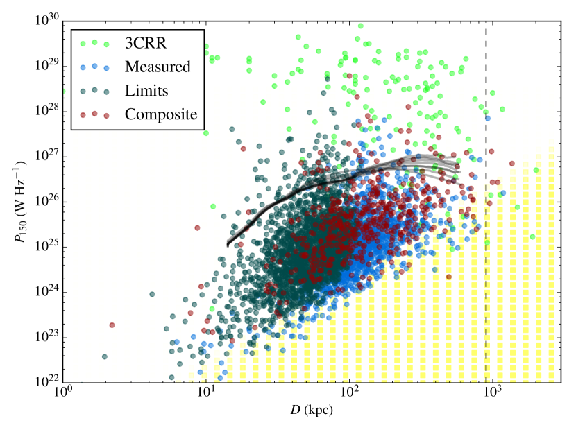
Figure 18: The power/linear-size diagram for AGN in our survey and for 3CRR objects. For the LOFAR AGN, we plot separately sources with angular sizes smaller than 15 arcsec as measured by pybdsm, where the physical sizes should probably be considered upper limits; sources with larger sizes, probably at least somewhat meaningfully measured by pybdsm: and composite sources, whose largest component separation is used as a proxy for their size. 3CRR sizes are all measured from high-resolution radio maps. Boxes indicate the region where some or all LOFAR sources in the range $z=0$ to $z=0.8$ with uniform surface brightness would drop below the detection threshold for our images. The vertical dashed line indicates our giant-radio-galaxy selection criterion (see the text for details). The grey curves represent tracks in the diagram for a source with a jet power of $10^{38}$ W, in various environments, derived from the modelling of Hardcastle & Krause (2014).

The radio power-linear size plot or $P$-$D$ diagram for radio-loud AGN, introduced by Baldwin (1982), is an important diagnostic of radio galaxy evolution. A new-born radio source will start at $P=0$, $D=0$ and (barring strong interactions with the external medium) is expected to have ${\rm d}D/{\rm d}t>0$ throughout its active lifetime, as the expansion of the source is driven by the ram pressure at the head of the jets: thus linear size is an important proxy of age, though the relationship between the two is determined by the source environment. The radio power is a function of the energy density in electrons and magnetic field in the lobes and of their volume, and so has a more complex relationship with source age, particularly when the effects of radiative losses are taken into account. Theoretical or numerical models of radio galaxy evolution (e.g., Kaiser et al. 1997; Blundell et al. 1999; Manolakou & Kirk 2002; Hardcastle & Krause 2013; Turner & Shabala 2015) predict tracks in the $P$-$D$ diagram for individual sources, depending on source environment and jet power; survey observations provide an instantaneous snapshot of the positions of many sources on their $P$-$D$ tracks. Observations of large samples can constrain models directly if they contain sources that are extreme with respect to the predicted tracks, e.g. very large or very powerful objects; more importantly, we may hope in future to use observed (multifrequency) radio power and size in large samples to infer properties such as jet power, age and environment on a per-source basis from the theoretical predictions. Inferring these properties for the large samples of radio-loud AGN expected to be generated by next-generation radio surveys, including those with LOFAR, will provide crucial input into our understanding of the ‘feedback’ processes believed to control the evolution of the most massive galaxies, as discussed in Section 1.

To construct a $P$-$D$ diagram clearly estimates of both $P$ and $D$ are necessary, i.e. in observational terms we need measurements of radio flux density, largest angular size and redshift. We have estimates of the angular sizes of our sources from the cataloguing process, but these need to be treated with caution for several reasons. As discussed in Section 3.4, the deconvolved major axes estimated by pybdsm for objects fitted with a single Gaussian tend to be overestimates, as small residual phase errors or offsets between the different spectral windows will make a source that is really unresolved to LOFAR appear marginally resolved in the images. For this reason, we consider all deconvolved sizes $<15$ arcsec to be unreliable, where the threshold is chosen based on the distribution of apparent source sizes and on visual inspection of the images. For sources where pybdsm associates more than one component, the size estimates are probably slightly more reliable, but these are a minority. For sources associated by us, we record the largest angular separation between the pybdsm positions of any pair of components, but this is only a crude estimate of the true angular size, being most reliable for edge-brightened FRII-type sources. All of these automatically generated sizes would benefit from verification by human inspection. Nevertheless they provide an interesting starting point for consideration of the sample power/linear-size plot. This is shown for the sources classed as AGN in Fig. 18. We overlay on this plot the equivalent values for the 3CRR sample (Laing et al., 1983), which, with its flux density limit of 10.9 Jy at 178 MHz, represents the most luminous radio AGN in the Universe at any particular redshift; it can be seen that there is significant overlap between the two, unsurprising since a number of 3CRR sources are present in our survey, but that, also as expected, the LOFAR survey picks up many more low-luminosity AGN. We also overlay, for illustrative purposes only, the theoretical tracks for a source with a jet power of $10^{38}$ W in various different environments for sizes between 10 and 600 kpc, taking account of radiative losses, derived from the MHD simulations of Hardcastle & Krause (2014), which, if accurate, indicate that the most luminous large sources seen in the LOFAR survey have jet powers around the value simulated in that work; however, some of the luminous, compact sources we see in the LOFAR surveys with $D\la 20$ kpc, $P\approx 10^{27}$ W Hz^-1 may well be young sources with significantly higher jet power that will eventually evolve, if their jets remain active, to 3CRR-like luminosities of $10^{28}$ – $10^{29}$ W Hz^-1. Thus we see the potential of the LOFAR data to allow us to construct a true jet kinetic luminosity function over several orders of magnitude in jet power, something we expect to return to in future papers.

Also plotted in Fig. 18 are the expected regions where sources cannot be detected, given the surface brightness limits at full resolution and sensitivity, and on the assumption of uniform source surface brightness, considering the redshift range 0–0.8 in which most of our sources lie. We see that we are capable of detecting (and do detect) sources with $\sim 100$-kpc sizes down to almost the lowest radio luminosities at which we detect AGN, but we expect to be significantly biased against low-luminosity large sources because of our surface brightness limitations. At high radio luminosities, we would expect to be able to detect all but the most extreme giant radio galaxies, where we adopt the standard definition in which the projected linear size of a giant is $>1$ Mpc. Giant radio galaxies are of particular interest because they represent one of the extremes in $P$-$D$ space: they must be particularly long-lived sources and their very existence places constraints on models of e.g. the possible active lifetime of jets. For this reason a number of searches for giant sources in existing low-frequency surveys have been carried out (e.g. Cotter et al., 1996; Lara et al., 2001; Machalski et al., 2001; Schoenmakers et al., 2001). Such searches have generally used large angular size as a proxy for giant status, and then followed up optically and/or with spectroscopy to identify physically large sources, thus favouring low-redshift giants. For example, Lara et al. (2001) find a sky density of 1 giant per $\sim 300$ square degrees, with an initial selection criterion of an angular size exceeding 4 arcmin in NVSS.

Our optically identified sample and the fact that we are capable of detecting powerful giants allows a direct approach to the problem. As Fig. 18 shows, we do detect 7 sources with sizes $\sim 1$ Mpc: in counting these we use a selection at 900 kpc to allow for the fact that the angular size values from component association are generally slightly underestimated, since they are the separations between the centres of the associated components, not their edges. Of these 7, all but one seem likely to be bona fide powerful giants (see Appendix A), implying a density of such $P\ga 3\times 10^{26}$ W Hz^-1 sources on the sky of at least 1 per 20 square degrees. These are, of course, only the optically identified giants, and we would expect to be biased against optical IDs of luminous sources, which will tend to be at high redshift, as well as of large sources, which are inherently difficult to identify. Our smallest (in angular size) giant is 140 arcsec in length, and there are a further 10 composite sources with sizes $>2$ arcmin in the associated catalogue, many of which may be high-$z$ giants. Although the numbers are small, these are substantially higher sky densities than were found by Lara et al. (2001), and suggest that the Tier 1 surveys will be a fruitful hunting ground for giant sources.

The surface brightness limitations in these full-resolution observations suggest that it would be useful to re-image the facet-calibrated data at low resolution (20–30 arcsec) to allow a search for low-surface brightness sources: Saripalli et al. (2012) have found a high detection rate of relatively low-luminosity large sources in a small sky area with good surface brightness sensitivity. As noted above, measurements of the numbers of giants as a function of radio luminosity and redshift provide important constraints on models of radio source evolution, and we plan to revisit the implications of the population of large sources in the LOFAR surveys in a future paper.

5.6 Remnant AGN

One of the key uncertainties in AGN evolution models is what happens when the jets are switched off. At this point, about half the energy that has ever been transported up the jets remains in the lobes, at least for powerful double objects (Hardcastle & Krause, 2013) and so the question of whether, and where, that energy is transferred to the external medium is one of great interest. However, the detection of sources in the post-switch-off phase, so-called remnant or relic AGN, has been surprisingly difficult. There are some well-known objects that appear to have no current AGN activity, for example B2 0924+30 (Cordey, 1987) or 3C 319 (Hardcastle et al., 1997), showing no flat-spectrum arcsec-scale core (the self-absorbed base of a currently active jet) and, where data are available, no AGN activity at any other waveband. But such objects are rare (Giovannini et al., 1988), making up no more than 7 per cent of the low-frequency classical double (FRII) population selected from 3CRR at $z<1.0$, for example (Mullin et al., 2008), though this fraction may be environment-dependent (Murgia et al., 2011). In fact true remnants, where AGN activity has completely ceased, seem to be somewhat rarer than double-double or restarting radio galaxies (Schoenmakers et al., 2000; Saripalli et al., 2012) despite the fact that double-doubles should be a fairly short-lived phenomenon as the newly active lobes will merge into the pre-existing plasma (Konar et al., 2013; Konar & Hardcastle, 2013), implying a very rapid fading process for remnants (cf. Kaiser & Cotter 2002). To date, however, statistical information on the remnant population has mainly come from studies of bright flux-limited samples like 3CRR, and as radio galaxies are expected to fade significantly as they age due to the effects of adiabatic expansion and radiative losses, it is clear that such samples may be biased against remnant sources.

It has long been suggested that remnant or relic AGN would have steep spectra (e.g. Parma et al., 2007; Murgia et al., 2011) and so would be detectable in greater numbers in sensitive surveys of the low-frequency sky. LOFAR should be extremely sensitive to remnant AGN, which are also expected to be physically large. Brienza et al. (2016a) set out possible methods for identifying remnant AGN in LOFAR fields, which include spectral selection (i.e., looking for steep-spectrum sources), morphological selection (looking for sources with little or no compact structure) and what might be termed core selection (looking for sources with no identifiable radio core). Each of these methods has its advantages and disadvantages. Brienza et al. (2016a) show that morphological selection appears to be more efficient in the Lockman Hole field than spectral selection, for the criteria they use, and one morphologically selected remnant in another LOFAR field has been followed up in detail, confirming its remnant nature (Brienza et al., 2016b). However, it is possible that remnants with recently switched off AGN would be missed by both the morphological and spectral selection methods; by contrast, all genuine remnant sources, whatever their age, would be expected to have no nuclear jet and so no arcsec-scale, flat-spectrum core. As an initial test for the efficiency of remnant surveys using this core selection criterion at Tier 1 depth and resolution, we have selected from the identified catalogue all sources which are (1) bright (total flux density $>80$ mJy at 150 MHz), ensuring that the sample is flux-complete across the survey region and that there is a good chance of seeing a core at high frequency, (2) well resolved ($>40$ arcsec), and (3) classed as AGN on the radio/FIR relation, for an initial visual search for remnants.

Of 127 such objects (after removing a few objects where it is doubtful that they are truly extended), we can see no evidence for a currently active core in the FIRST images in 38, a potential remnant fraction of 30 per cent. Examples of candidate remnant sources, together with some comparable sources where a FIRST core is seen, are shown in Appendix B. We do not include in our remnant count any source where FIRST emission is coincident with the optical ID, even if there is no clear evidence of a point source; so the true remnant fraction could be slightly higher than we quote above. Sources without a core in FIRST are also less likely to be optically identified, hence again biasing our estimate low. On the other hand, we do not exclude sources on the basis of showing apparent compact hotspots in the FIRST images. Even if truly compact, something we cannot really assess on the basis of the FIRST images, such features may persist for more than a light-travel time along the lobes after the jet turns off, and so do not imply that the jet is still active. The fact that the fraction we measure is higher than for 3CRR sources is consistent with the idea that remnants might be more detectable in more sensitive surveys, although it is clear that remnants do not dominate the LOFAR sky at these flux density levels.

The main limitation on this conclusion is the fact that the FIRST images are not particularly sensitive to cores. If we define the core prominence as the ratio of core flux density at 1.4 GHz [the exact frequency is unimportant since radio galaxy core spectra are flat up to high frequencies: (e.g. Hardcastle & Looney, 2008; Whittam et al., 2013)] to total flux density at 150 MHz, then FIRST’s $3\sigma$ upper limit on core prominence for the faintest objects corresponds to $0.4/80=5\times 10^{-3}$, while we know that the median core prominence for 3CRR objects with detected cores is $\sim 3\times 10^{-4}$ (Mullin et al., 2008). 3CRR objects are selected to be the brightest low-frequency sources on the sky and would be expected to have systematically low prominences, so this is an unfair comparison, but clearly it is possible that even moderately faint radio cores are escaping detection in our calculation of the remnant fraction above. We therefore regard the remnant fraction we have derived above as an upper limit. Even so, such a limit is interesting, as it requires the typical fading timescale for remnants at 150 MHz to be at most $\sim 30$ per cent of the active time. Sensitive radio followup of remnant candidates will be necessary to constrain the remnant fraction further.

A power/linear-size diagram for the 80-mJy, 40-arcsec subsample (Fig. 19) shows that the remnant candidates do not occupy any particularly special position with respect to the cored sources, but there is a slight tendency for them to have lower radio luminosity for a given size, in the sense that all remnant candidates with sizes $>300$ kpc, and many of those below that size, lie at the very lowest end of the radio luminosity distribution. This would support the idea that remnants fade rapidly even at low frequencies once the jets switch off. There is no apparent difference between the in-band spectral indices of the two samples, but as noted above, these are very unreliable, and some remnants by our definition would be expected to have flat radio spectra anyway. We defer an investigation of the LOFAR/NVSS spectral index for the bright identified sample to a future paper, as this will require individual measurements from LOFAR and NVSS maps for all sources.

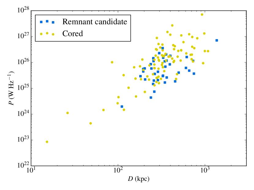
Figure 19: The power/linear size diagram for the bright, resolved subsample discussed in the text.

6 Summary and conclusions

We have presented details of the observations, data reduction and quality assessment for a survey consisting of four LOFAR HBA pointings in the H-ATLAS NGP area. Although this survey does not have uniform noise, it is otherwise expected to be reasonably representative in data quality of the much larger ‘Tier 1’ survey currently being carried out by the LOFAR Surveys Key Science project. Key points from the discussion of the data reduction and quality assessment are as follows:

• We have been able to image over 140 square degrees at 150 MHz at a resolution of better than 10 arcsec and with rms noise in the broad-band 150-MHz maps ranging between 100 $\mu$Jy beam^-1 and $\sim 2$ mJy beam^-1, thus covering almost all of the NGP field as surveyed by H-ATLAS. The fact that this can be done in a total of 34 hours’ observing illustrates the capabilities of LOFAR for wide-area, deep surveys.

• The LOFAR flux scale remains problematic. The method we have developed to calibrate flux densities in the field – by cross-matching a large number of objects to existing low-frequency catalogues (Section 3.2) – works well so long as there are enough objects in existing catalogues to make a statistical comparison possible, but this is not the case for the whole sky.

• Even after correcting as well as possible for the flux scale issues, HBA in-band spectral indices are unreliable because of the limited frequency range spanned by the data, to the extent that these are unlikely to be useful for all but the brightest sources (Section 4.5). However, reasonable HBA/NVSS spectral index distributions are obtained for compact sources (Section 4.6).

• Per-facet positional offsets introduced by the self-calibration in facet calibration are small but can be significant in poor-quality data. Perhaps more significant is the effect that we take to be the residual blurring of sources by inadequate phase calibration, leading to a loss of peak flux density and incompleteness at low flux densities (Section 3.4). This may be exacerbated for us by the image-plane combination of multiple spectral windows.

For data reduction of the Tier 1 surveys it would probably be preferable to carry out our flux scaling method before facet calibration, which would then allow the facet calibration to be run using all bands simultaneously as described by vW16 while still having correct flux densities. In-band spectral indices, if desired, could be derived by re-imaging after facet calibration. It is not yet clear whether the facet-based approach of vW16 is fundamentally limited in terms of the calibration quality that can be achieved away from the calibration point, i.e. whether some sort of phase screen interpolation or an algorithm that can fit to much smaller facets will be required. Nevertheless, the technique represents a significant advance towards the exploitation of LOFAR’s capabilities and in this paper we have demonstrated that applying it to large areas is technically and computationally feasible.

We have also constructed an optically identified catalogue using SDSS galaxy catalogues and spectroscopy, and have used it to investigate the science that can be done with a combination of LOFAR, SDSS and Herschel data. Some key points from this analysis are as follows:

• We achieve a roughly 40 per cent optical identification rate for the LOFAR catalogue using SDSS together with FIRST to assist with identifications (Section 3.5). This is the result of a labour-intensive process in which the vast majority of sources were visually inspected in several bands [a similar approach for the Boötes field will be described by Williams et al. (2016b)]. Clearly if this process is to be scaled up to the many hundreds of LOFAR pointings already in hand in Tier 1, it will require significant automation. On the other hand, the catalogues would benefit from further visual inspection, for example to provide quality checks on large sources found by pybdsm and to measure flux density and source size more accurately. Generating high-quality catalogues from Tier 1 data will remain labour-intensive even if some of the optical identification process can be streamlined.

• It is important to note that there are many resolved sources without optical IDs, and, as discussed in Section 5.6, many of these may not have radio cores in FIRST. This may represent a challenge for spectroscopic followup projects such as WEAVE-LOFAR (Smith, 2015) which rely on accurate positions for their targets.

• Comparing with the H-ATLAS images, we recover the well-known radio/FIR relation in flux/flux and luminosity/luminosity plots using the 250-$\mu$m Herschel data (Sections 5.2, 5.3) but see evidence that there is a population of radio-faint SFGs with radio flux densities well below their expected values on this correlation, consistent with earlier empirical work (Smith et al., 2014). On the other hand, we are able to use the fact that sources with larger radio luminosities than would be expected from their FIR emission must be radio-loud AGN to perform an efficient SFG/AGN separation in the optically identified catalogue. Radio source count analysis not only shows consistency with existing 150-MHz determinations where available (Section 5.1) but, for the SFGs, shows good agreement (Section 5.3) with the widely used models of Wilman et al. (2008).

• We present a 150-MHz radio luminosity function derived from $\sim 2,000$ objects with $r<19$ mag, which shows good agreement with the expectations from higher frequencies (Section 5.4). Strong luminosity function evolution with redshift is seen for the SFGs.

• The power/linear-size diagram for the overall sample (Section 5.5) shows that we are still insensitive to very large sources at low radio luminosities, something which may need to be addressed in Tier 1 data processing by an additional imaging step at low resolution. However, we measure a sky density of genuine optically identified powerful giant radio galaxies ($L_{\rm 150}\ga 10^{26}$ W Hz^-1, $D\ga 1$ Mpc) which is high compared to some estimates in the literature, thanks to our good optical identification rate out to relatively high redshifts.

• We carry out an initial search for candidate remnant sources, where the jets have switched off, in a bright, resolved subsample (Section 5.6). Up to 30 per cent of the sample sources show no FIRST core, which might imply a lifetime in the remnant phase comparable to that in the active phase. However, many of these remnant candidates may have radio cores below the FIRST detection limit: sensitive high-frequency observations will be necessary to refine the upper limit on remnants in LOFAR samples.

Subsequent papers will address many of these points in more detail.

Appendix A They might be giants

Fig. 20 shows postage stamps of the 7 objects discussed in Section 5.5 as candidate optically identified giants in the field. Of these, only one (the one identified with SDSS J133744.35+2513359.0) seems likely to be spurious. This is one of the two non-composite sources of the seven and its large size is a result of pybdsm associating it with a large region of low-surface-brightness emission. Further investigation with low-resolution imaging would be required to say whether the extended emission is really associated with the LOFAR source. All the remaining 6 objects are clear double radio sources. Most of the optical identifications are unambiguous, and the source identified with SDSS J132735.32+350636.7, which is less certain, is identified with the brightest plausible galaxy in a crowded field and so is unlikely to be at lower redshift. Three of the optical identifications (SDSS J133127.82+250050.0, SDSS J134415.75+331719.1, SDSS J130451.41+245445.9) are quasars with spectroscopic redshifts; they are therefore likely substantially larger in physical size than they appear. SDSS J131443.83+273741.3 is a radio galaxy with a spectroscopic redshift; the other redshifts are photometric.

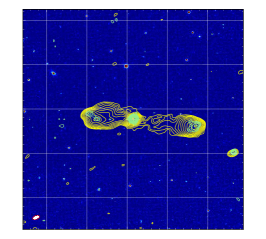
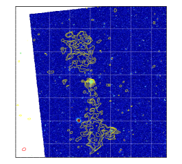
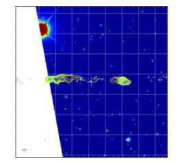
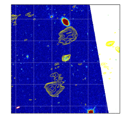
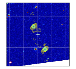
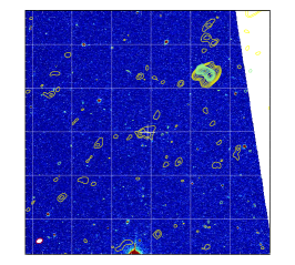
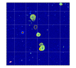
Figure 20: ‘Postage stamp’ images of the 7 optically identified objects at or close to 1 Mpc in physical size in the sample. Colours show SDSS $r$-band images: contours are LOFAR (yellow) and FIRST (green) contours starting at the local 3$\sigma$ value and increasing by steps of a factor 2. An ellipse in the bottom left-hand corner shows the LOFAR beam and a white cross the location of the optical identification. Grid lines are spaced by 1 arcmin in right ascension and declination: north is up. Top row, from left to right, are: SDSS J133127.82+250050.0 ($z=0.8040$, $D=0.9$ Mpc), J134415.75+331719.1 ($z=0.6863$, $D=1.0$ Mpc), and J130451.41+245445.9 ($z=0.6025$, $D=1.0$ Mpc). Middle row: J132928.99+333810.1 ($z=0.5404$, $D=1.0$ Mpc), and J132735.32+350636.7 ($z=0.5003$, $D=1.4$ Mpc), J133744.35+251359.0 ($z=0.6816$, $D=1.2$ Mpc). Bottom: J131443.83+273741.3 ($z=0.4179$, $D=1.1$ Mpc).

Appendix B Remnants and non-remnants

Candidate remnant sources (Fig. 21) show a wide range of morphologies. Many of them have no compact emission in FIRST at all, though some have hotspots; as noted in the main text, the presence of hotspots does not in itself indicate that a source is not a recent remnant. Sources where double lobes cannot be distinguished are quite common (e.g. SDSS J130532.02+315634.8), as are sources like SDSS J134802.70+322940.1 where LOFAR surface brightness sensitivity at full resolution limits our ability to image the source structure. These may be examples of the ‘relaxed double’ class (Leahy, 1993). There are also a number of objects like SDSS J125147.03+314047.6 and SDSS J131405.90+243240.3, whose ‘inner hotspots’ may indicate a restarting source rather than a remnant radio galaxy. LOFAR provides a good opportunity for the study of restarting (double-double) sources (e.g. Orrù et al., 2015).

For comparison, and to illustrate the range of source structures seen, we plot some examples of sources from the 80-mJy subsample not classed as remnants in Fig. 22. As can be seen, core strength in these objects ranges from a dominant component in FIRST (e.g. in the quasar SDSS J133449.73+312824.0) to a weak extension of lobe emission over the optical ID (SDSS J134747.98+325823.8). Tailed morphology is seen in many of these (e.g. the wide-angle tail SDSS J130856.91+261333.2): we have not seen a convincing example of a tailed remnant candidate.

Figure 21: Postage stamps of example candidate remnant sources. Colours, contours and lines as in Fig. 20. From left to right, top to bottom: SDSS J125147.03+314047.6, J125311.62+304017.3, J125930.81+333646.9, J130004.25+263652.7, J130332.47+312949.5, J130532.02+315634.8, J130916.02+305121.9, J131040.03+322047.6, J131405.90+243240.3, J133057.34+351650.2, J133422.21+343634.8, and J134802.70+322940.1.

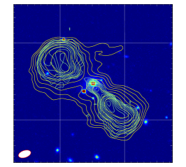
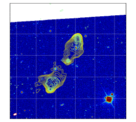
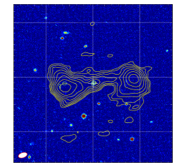
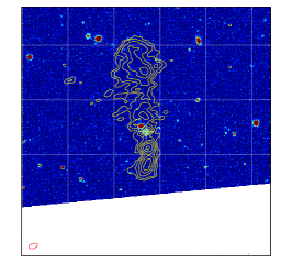
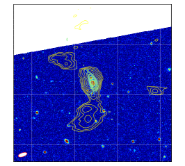
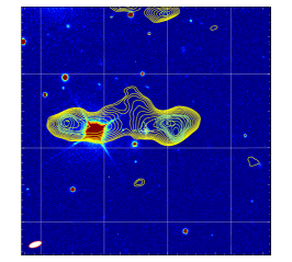
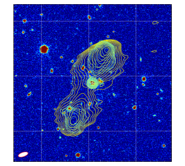
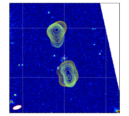
Figure 22: Postage stamps of example sources with FIRST cores. Colours, contours and lines as in Fig. 20. From left to right, top to bottom: SDSS J124541.96+332428.5, J125541.50+250744.7, J125715.99+312153.1, J130057.21+325625.5, J130856.91+261333.2, J131246.85+275219.8, J132713.87+285318.1, J133449.73+312824.0, J133738.33+312514.2, J133837.35+311413.8, J134251.68+311052.6, and J134747.98+325823.8.

REFERENCES

- Alam et al. (2015) Alam S., et al., 2015, ApJS, 219, 12
- Astropy Collaboration et al. (2013) Astropy Collaboration et al., 2013, A&A, 558, A33
- Baldwin (1982) Baldwin J. E., 1982, in Heeschen D. S., Wade C. M., eds, IAU Symposium Vol. 97, Extragalactic Radio Sources. pp 21–24
- Beck et al. (2016) Beck R., Dobos L., Budavári T., Szalay A. S., Csabai I., 2016, preprint, (arXiv:1603.09708)
- Becker et al. (1995) Becker R. H., White R. L., Helfand D. J., 1995, ApJ, 450, 559
- Best et al. (2005) Best P. N., Kauffmann G., Heckman T. M., Brinchmann J., Charlot S., Ivezić Z., White S. D. M., 2005, MNRAS, 362, 25
- Best et al. (2014) Best P. N., Ker L. M., Simpson C., Rigby E. E., Sabater J., 2014, MNRAS, 445, 955
- Blundell et al. (1999) Blundell K. M., Rawlings S., Willott C. J., 1999, AJ, 117, 677
- Bonfield et al. (2011) Bonfield D. G., et al., 2011, MNRAS, 416, 13
- Brienza et al. (2016a) Brienza M., Mahony E., Morganti R., Prandoni I., Godfrey L., 2016a, preprint, (arXiv:1603.01837)
- Brienza et al. (2016b) Brienza M., et al., 2016b, A&A, 585, A29
- Brown & Rudnick (2011) Brown S., Rudnick L., 2011, MNRAS, 412, 2
- Chilingarian et al. (2010) Chilingarian I. V., Melchior A.-L., Zolotukhin I. Y., 2010, MNRAS, 405, 1409
- Colla et al. (1973) Colla G., et al., 1973, A&AS, 11, 291
- Condon et al. (1998) Condon J. J., Cotton W. D., Greisen E. W., Yin Q. F., Perley R. A., Taylor G. B., Broderick J. J., 1998, AJ, 115, 1693
- Condon et al. (2002) Condon J. J., Cotton W. D., Broderick J. J., 2002, AJ, 124, 675
- Cordey (1987) Cordey R. A., 1987, MNRAS, 227, 695
- Cotter et al. (1996) Cotter G., Rawlings S., Saunders R., 1996, MNRAS, 281, 1081
- Croton et al. (2006) Croton D., et al., 2006, MNRAS, 365, 111
- Cruz et al. (2006) Cruz M. J., et al., 2006, MNRAS, 373, 1531
- Dawson et al. (2013) Dawson K. S., et al., 2013, AJ, 145, 10
- Driver et al. (2009) Driver S. P., et al., 2009, Astronomy and Geophysics, 50, 050000
- Driver et al. (2011) Driver S. P., et al., 2011, MNRAS, 413, 971
- Dunne et al. (2011) Dunne L., et al., 2011, MNRAS, 417, 1510
- Dye et al. (2010) Dye S., et al., 2010, A&A, 518, L10
- Eales (1985) Eales S. A., 1985, MNRAS, 213, 899
- Eales et al. (2010) Eales S., et al., 2010, PASP, 122, 499
- Eisenstein et al. (2011) Eisenstein D. J., et al., 2011, AJ, 142, 72
- Foreman-Mackey et al. (2013) Foreman-Mackey D., Hogg D. W., Lang D., Goodman J., 2013, PASP, 125, 306
- Giovannini et al. (1988) Giovannini G., Feretti L., Gregorini L., Parma P., 1988, A&A, 199, 73
- Griffin et al. (2010) Griffin M. J., et al., 2010, A&A, 518, L3
- Gruppioni et al. (2013) Gruppioni C., et al., 2013, MNRAS, 432, 23
- Gürkan et al. (2015) Gürkan G., et al., 2015, MNRAS, 452, 3776
- Haarsma et al. (2000) Haarsma D. B., Partridge R. B., Windhorst R. A., Richards E. A., 2000, ApJ, 544, 641
- Hales et al. (1988) Hales S. E. G., Baldwin J. E., Warner P. J., 1988, MNRAS, 234, 919
- Hales et al. (2007) Hales S. E. G., Riley J. M., Waldram E. M., Warner P. J., Baldwin J. E., 2007, MNRAS, 382, 1639
- Hardcastle & Krause (2013) Hardcastle M. J., Krause M. G. H., 2013, MNRAS, 430, 174
- Hardcastle & Krause (2014) Hardcastle M. J., Krause M. G. H., 2014, MNRAS, 443, 1482
- Hardcastle & Looney (2008) Hardcastle M. J., Looney L. W., 2008, MNRAS, 388, 176
- Hardcastle et al. (1997) Hardcastle M. J., Alexander P., Pooley G. G., Riley J. M., 1997, MNRAS, 288, 859
- Hardcastle et al. (2007) Hardcastle M. J., Croston J. H., Kraft R. P., 2007, ApJ, 669, 893
- Hardcastle et al. (2009) Hardcastle M. J., Evans D. A., Croston J. H., 2009, MNRAS, 396, 1929
- Hardcastle et al. (2010) Hardcastle M. J., et al., 2010, MNRAS, 409, 122
- Hardcastle et al. (2013) Hardcastle M. J., et al., 2013, MNRAS, 429, 2407
- Heald et al. (2015) Heald G. H., et al., 2015, A&A, 582, A123
- Helou et al. (1985) Helou G., Soifer B. T., Rowan-Robinson M., 1985, ApJ, 298, L7
- Hopkins & Beacom (2006) Hopkins A. M., Beacom J. F., 2006, ApJ, 651, 142
- Ibar et al. (2008) Ibar E., et al., 2008, MNRAS, 386, 953
- Ibar et al. (2009) Ibar E., Ivison R. J., Biggs A. D., Lal D. V., Best P. N., Green D. A., 2009, MNRAS, 397, 281
- Ibar et al. (2010) Ibar E., et al., 2010, MNRAS, 409, 38
- Intema et al. (2016) Intema H. T., Jagannathan P., Mooley K. P., Frail D. A., 2016, preprint, (arXiv:1603.04368)
- Ivison et al. (2010a) Ivison R. J., et al., 2010a, MNRAS, 402, 245
- Ivison et al. (2010b) Ivison R. J., et al., 2010b, A&A, 518, L31
- Jarvis et al. (2010) Jarvis M. J., et al., 2010, MNRAS, 409, 92
- Kaiser & Cotter (2002) Kaiser C. R., Cotter G., 2002, MNRAS, 336, 649
- Kaiser et al. (1997) Kaiser C. R., Dennett-Thorpe J., Alexander P., 1997, MNRAS, 292, 723
- Kalfountzou et al. (2014) Kalfountzou E., et al., 2014, MNRAS, 442, 1181
- Karim et al. (2011) Karim A., et al., 2011, ApJ, 730, 61
- Konar & Hardcastle (2013) Konar C., Hardcastle M. J., 2013, MNRAS, 436, 1595
- Konar et al. (2013) Konar C., Hardcastle M. J., Jamrozy M., Croston J. H., 2013, MNRAS, 430, 2137
- Lacki et al. (2010) Lacki B. C., Thompson T. A., Quataert E., 2010, ApJ, 717, 1
- Laing et al. (1983) Laing R. A., Riley J. M., Longair M. S., 1983, MNRAS, 204, 151
- Lane et al. (2014) Lane W. M., Cotton W. D., van Velzen S., Clarke T. E., Kassim N. E., Helmboldt J. F., Lazio T. J. W., Cohen A. S., 2014, MNRAS, 440, 327
- Lara et al. (2001) Lara L., Cotton W. D., Feretti L., Giovannini G., Marcaide J. M., Márquez I., Venturi T., 2001, A&A, 370, 409
- Leahy (1993) Leahy J. P., 1993, in Röser H.-J., Meisenheimer K. ed., Jets in Extragalactic Radio Sources. Springer-Verlag, Heidelberg, p. 1
- Lindsay et al. (2014) Lindsay S. N., et al., 2014, MNRAS, 440, 1527
- Machalski & Godlowski (2000) Machalski J., Godlowski W., 2000, A&A, 360, 463
- Machalski et al. (2001) Machalski J., Jamrozy M., Zola S., 2001, A&A, 371, 445
- Madau et al. (1996) Madau P., Ferguson H. C., Dickinson M. E., Giavalisco M., Steidel C. C., Fruchter A., 1996, MNRAS, 283, 1388
- Magnelli et al. (2013) Magnelli B., et al., 2013, A&A, 553, A132
- Mancuso et al. (2015) Mancuso C., et al., 2015, ApJ, 810, 72
- Manolakou & Kirk (2002) Manolakou K., Kirk J. G., 2002, A&A, 391, 127
- Mauch & Sadler (2007) Mauch T., Sadler E., 2007, MNRAS, 375, 931
- Mauch et al. (2013) Mauch T., Klöckner H.-R., Rawlings S., Jarvis M., Hardcastle M. J., Obreschkow D., Saikia D. J., Thompson M. A., 2013, MNRAS, 435, 650
- McAlpine et al. (2013) McAlpine K., Jarvis M. J., Bonfield D. G., 2013, MNRAS, 436, 1084
- Mohan & Rafferty (2015) Mohan N., Rafferty D., 2015, PyBDSM: Python Blob Detection and Source Measurement, Astrophysics Source Code Library (ascl:1502.007)
- Mullin et al. (2008) Mullin L. M., Riley J. M., Hardcastle M. J., 2008, MNRAS, 390, 595
- Murgia et al. (2011) Murgia M., et al., 2011, A&A, 526, A148
- Murphy (2009) Murphy E. J., 2009, ApJ, 706, 482
- Offringa et al. (2014) Offringa A. R., et al., 2014, MNRAS, 444, 606
- Orrù et al. (2015) Orrù E., et al., 2015, A&A, 584, A112
- Pandey et al. (2009) Pandey V. N., van Zwieten J. E., de Bruyn A. G., Nijboer R., 2009, in Saikia D. J., Green D. A., Gupta Y., Venturi T., eds, Astronomical Society of the Pacific Conference Series Vol. 407, The Low-Frequency Radio Universe. p. 384
- Parma et al. (2007) Parma P., Murgia M., de Ruiter H. R., Fanti R., Mack K.-H., Govoni F., 2007, A&A, 470, 875
- Pascale et al. (2011) Pascale E., et al., 2011, MNRAS, 415, 911
- Pilbratt et al. (2010) Pilbratt G. L., et al., 2010, A&A, 518, L1
- Poglitsch et al. (2010) Poglitsch A., et al., 2010, A&A, 518, L2
- Pracy et al. (2016) Pracy M., et al., 2016, preprint, (arXiv:1604.04332)
- Prescott et al. (2016) Prescott M., et al., 2016, MNRAS, 457, 730
- Rawlings et al. (2001) Rawlings S., Eales S., Lacy M., 2001, MNRAS, 322, 523
- Rigby et al. (2011) Rigby E. E., et al., 2011, MNRAS, 415, 2336
- Röttgering et al. (2006) Röttgering H. J. A., et al., 2006, ArXiv Astrophysics e-prints,
- Saripalli et al. (2012) Saripalli L., Subrahmanyan R., Thorat K., Ekers R. D., Hunstead R. W., Johnston H. M., Sadler E. M., 2012, ApJS, 199, 27
- Scaife & Heald (2012) Scaife A. M. M., Heald G. H., 2012, MNRAS, 423, L30
- Schlafly & Finkbeiner (2011) Schlafly E. F., Finkbeiner D. P., 2011, ApJ, 737, 103
- Schoenmakers et al. (2000) Schoenmakers A. P., de Bruyn A. G., Röttgering H. J. A., van der Laan H., Kaiser C. R., 2000, MNRAS, 315, 371
- Schoenmakers et al. (2001) Schoenmakers A. P., de Bruyn A. G., Röttgering H. J. A., van der Laan H., 2001, A&A, 374, 861
- Serjeant et al. (2010) Serjeant S., et al., 2010, A&A, 518, L7
- Seymour et al. (2008) Seymour N., et al., 2008, MNRAS, 386, 1695
- Simpson et al. (2012) Simpson C., et al., 2012, MNRAS, 421, 3060
- Smith (2015) Smith D. J. B., 2015, preprint, (arXiv:1506.05630)
- Smith et al. (2013) Smith D. J. B., et al., 2013, MNRAS, 436, 2435
- Smith et al. (2014) Smith D. J. B., et al., 2014, MNRAS, 445, 2232
- Smolčić et al. (2009) Smolčić V., et al., 2009, ApJ, 690, 610
- Sutherland & Saunders (1992) Sutherland W., Saunders W., 1992, MNRAS, 259, 413
- Tasse et al. (2013) Tasse C., van der Tol S., van Zwieten J., van Diepen G., Bhatnagar S., 2013, A&A, 553, A105
- Taylor (2005) Taylor M. B., 2005, in Shopbell P., Britton M., Ebert R., eds, Astronomical Society of the Pacific Conference Series Vol. 347, Astronomical Data Analysis Software and Systems XIV. p. 29
- Turner & Shabala (2015) Turner R. J., Shabala S. S., 2015, ApJ, 806, 59
- Virdee et al. (2013) Virdee J. S., et al., 2013, MNRAS, 432, 609
- Whittam et al. (2013) Whittam I. H., et al., 2013, MNRAS, 429, 2080
- Williams et al. (2016) Williams W. L., et al., 2016, preprint, (arXiv:1605.01531)
- Willott et al. (1999) Willott C. J., Rawlings S., Blundell K. M., Lacy M., 1999, MNRAS, 309, 1017
- Willott et al. (2002) Willott C. J., Rawlings S., Archibald E. N., Dunlop J. S., 2002, MNRAS, 331, 435
- Wilman et al. (2008) Wilman R. J., et al., 2008, MNRAS, 388, 1335
- Yun et al. (2001) Yun M. S., Reddy N. A., Condon J. J., 2001, ApJ, 554, 803
- Zwart et al. (2014) Zwart J. T. L., Jarvis M. J., Deane R. P., Bonfield D. G., Knowles K., Madhanpall N., Rahmani H., Smith D. J. B., 2014, MNRAS, 439, 1459
- de Jong et al. (1985) de Jong T., Klein U., Wielebinski R., Wunderlich E., 1985, A&A, 147, L6
- van Haarlem et al. (2013) van Haarlem M. P., et al., 2013, A&A, 556, A2
- van Weeren et al. (2016) van Weeren R. J., et al., 2016, ApJS, 223, 2
- van der Kruit (1971) van der Kruit P. C., 1971, A&A, 15, 110