An efficiently and tunable switch between slow- and fast- light in double mode with an optomechanical system

Abstract

We study the dynamics of a driven optomechanical cavity coupled to a charged nanomechanical resonator via Coulomb interaction. We find the tunable switch between slow- and fast- light in double-mode can be observed from the output field by adjusting the laser-cavity detuning in this coupled system. Moreover, the requencies of signal light can be tuned by Coulomb coupling strength. The proposal may have potential application in optical communcation and nonlinear optics.

1 Introduction

The control of slow and fast light propagation is a challenging task. Research on slow- and fast- light systems has increased from both theoretical and experimental aspects in physics [1, 2]. The first superluminal light propagation was observed in a resonant system [3], where the laser propagates without appreciable shape distortion but experiences very strong resonant absorption. Various techniques have been developed to realized slow and fast light in atomic vapors [4, 5, 6] and solid materials [7, 8]. To reduce absorption, most of those works [4, 5, 6, 7] are based on the electromagnetically induced transparency (EIT) or coherent population oscillation (CPO) [9].

On the other hand, opto-mechanical [10, 11, 12, 13, 14, 15] systems have advanced rapidly, which are promising candidates for realizing architectures exhibiting quantum behavior in macroscopic structures. Also, a lot of them have been demonstrated experimentally in this systems, for example, quantum information transfer [16], normal mode splitting [14, 17], optomechanically induced transparency (OMIT) [18], frequency transfer [19]. Slow- and fast- light also has been successfully observed in this system [20], where an optically tunable delay of 50 ns with near-unity optical transparency and superluminal light with a 1.4-$\mu$s signal advance. Most recently proposals are proposed in this system, such as slow light based on an optomechanical cavity with a Bose-Einstein condensate (BEC) [21] and fast light in reflection meanwhile slow light in transmission [22]. Moreover, we have demonstrated an efficient switch between slow and fast light in microwave regime [23].

However, above proposals and experiments all are work in one optical mode. In this paper, we theoretically investigate the slow- and fast- light in double light mode based on the optomechanical system. Compare to resent proposal [20, 21, 22], we can efficiently switch from slow- to fast- light in double light mode only by adjusting the effective laser-cavity detuning in reflective light. Moreover, the frequency of output light can be tunable according to Coulomb coupling strength

This paper is structured as follows. In Sec. 2 we present the model and the analytical expressions of the optomechanical system and obtain the solutions. Sec. 3 includes numerical calculations for the efficiently double mode and tunable switch from slow to fast based on recent experimental parameters. The last section is a brief conclusion.

2 Model and solutions

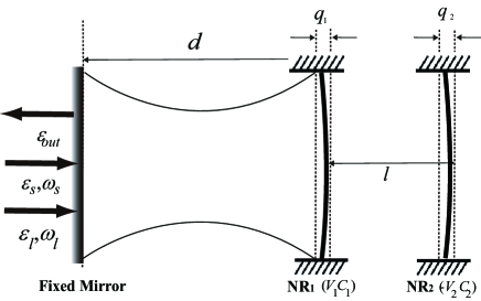
Figure 1: (Color online) Schematic diagram of the system. A high-quality Fabry-Pérot cavity consists of a fixed mirror and a movable mirror NR₁. NR₁ is charged by the bias gate voltage $V_{1}$ and subject to the Coulomb force due to another charged NR₂ with the bias gate voltage $-V_{2}$. The optomechanical cavity of the length $d$ is driven by two light fields, one of which is the pump field $\varepsilon_{l}$ with frequency $\omega_{l}$ and the other of which is the probe field $\varepsilon_{s}$ with frequency $\omega_{s}$. The output field is represented by $\varepsilon_{out}$. $q_{1}$ and $q_{2}$ represent the small displacements of NR₁ and NR₂ from their equilibrium positions, with $l$ is the equilibrium distance between the two NRs.

We begin with the Hamiltonian of the opto-mechanical system. As shown schematically in Fig. 1, the Hamiltonian is given by [24],

$$H=\hbar\omega_{a}a^{{\dagger}}a+(\frac{p_{1}^{2}}{2m_{1}}+\frac{1}{2}m_{1}\omega_{1}^{2}q_{1}^{2})$$

$$+(\frac{p_{2}^{2}}{2m_{2}}+\frac{1}{2}m_{2}\omega_{2}^{2}q_{2}^{2})-\hbar ga^{{\dagger}}aq_{1}+\hbar\lambda q_{1}q_{2}$$

$$+i\hbar\varepsilon_{l}(a^{{\dagger}}e^{-i\omega_{l}t}-H.c.)+i\hbar(a^{{\dagger}}\varepsilon_{s}e^{-i\omega_{s}t}-H.c.),$$ (1)

where the first term is for the single-mode cavity field with frequency $\omega_{a}$ and annihilation (creation) operator $a\ (a^{{\dagger}})$. The second (third) term describes the vibration of the charged NR₁ (NR₂ ) with frequency $\omega_{1}$ ($\omega_{2}$), effective mass $m_{1}$ ($m_{2}$), position $q_{1}$ ($q_{2}$) and momentum operator $p_{1}$ ($p_{2}$) [25]. The forth term denote the NR₁ couples to the cavity field due to the radiation pressure with the coupling strength $g=\frac{\omega_{a}}{d}$ with $d$ being the cavity length.

The fifth term presents the Coulomb coupling between the charged NR₁ and the charged NR₂ and $\lambda=\frac{C_{1}V_{1}C_{2}V_{2}}{2\pi\hbar\varepsilon_{0}r_{0}^{3}}$ [24, 26, 27], where the NR₁ and NR₂ take the charges $C_{1}V_{1}$ and $-C_{2}V_{2}$, with $C_{1}(C_{2})$ and $V_{1}(-V_{2})$ being the capacitance and the voltage of the bias gate, respectively. $l$ is the equilibrium distance between the two NRs. $q_{1}$ and $q_{2}$ represent the small displacements of NR₁ and NR₂ from their equilibrium positions, respectively. The last two terms in Eq. (1) describe the interactions between the cavity field and the two input fields, respectively. The strong (week) laser (signal) field owns the frequency $\omega_{l}$ ($\omega_{s}$) and the amplitude $\varepsilon_{l}=\sqrt{2\kappa\wp_{l}/\hbar\omega_{l}}$ ($\varepsilon_{s}=\sqrt{2\kappa\wp_{s}/\hbar\omega_{s}}$), whit $\wp_{l}$ ($\wp_{s}$) is the power of the laser (signal) field and $\kappa$ is the cavity decay rate.

In a frame rotating with the frequency $\omega_{l}$ of the laser field, the Hamiltonian of the system Eq.(1) can be rewritten as,

$$H=\hbar\Delta_{a}a^{\dagger}a+(\frac{p_{1}^{2}}{2m_{1}}+\frac{1}{2}m_{1}\omega_{1}^{2}q_{1}^{2})$$

$$+(\frac{p_{2}^{2}}{2m_{2}}+\frac{1}{2}m_{2}\omega_{2}^{2}q_{2}^{2})-\hbar ga^{\dagger}aq_{1}+\hbar\lambda q_{1}q_{2}$$

$$+i\hbar\varepsilon_{l}(a^{\dagger}-a)+i\hbar(a^{\dagger}\varepsilon_{s}e^{-i\delta t}-H.c.),$$ (2)

where $\Delta_{a}=\omega_{a}-\omega_{l}$ is the detuning of the laser field from the bare cavity, and $\delta=\omega_{s}-\omega_{l}$ is the detuning of the singal field from the laser field.

Considering photon losses from the cavity , we may describe the dynamics of the system governed by Eq. (2) using following nonlinear quantum Langevin equations [25],

$$\langle\dot{q_{1}}\rangle=\frac{\langle p_{1}\rangle}{m_{1}},$$

$$\langle\dot{p_{1}}\rangle=-m_{1}\omega_{1}^{2}\langle q_{1}\rangle-\hbar\lambda\langle q_{2}\rangle+\hbar g\langle c^{{\dagger}}\rangle\langle c\rangle-\gamma_{1}\langle p_{1}\rangle,$$

$$\langle\dot{q_{2}}\rangle=\frac{\langle p_{2}\rangle}{m_{2}},$$

$$\langle\dot{p_{2}}\rangle=-m_{2}\omega_{2}^{2}\langle q_{2}\rangle-\hbar\lambda\langle q_{1}\rangle-\gamma_{2}\langle p_{2}\rangle,$$

$$\langle\dot{a}\rangle=-[\kappa+i(\Delta_{a}-g\langle q_{1}\rangle)]\langle a\rangle+\varepsilon_{l}+\varepsilon_{s}e^{-i\delta t},$$ (3)

here $\gamma_{1}$ and $\gamma_{2}$ are the decay rates for NR₁ and NR₂, respectively. Where we have been considered: (i) The quantum Brownian noise $\xi_{1}$ $(\xi_{2})$ comes from the coupling between NR₁ (NR₂) and its own environment with zero mean value [28]; (ii) $c_{in}$ is the input vacuum noise operator with zero mean value [28] and under the mean field approximation $\langle Qa\rangle=\langle Q\rangle\langle a\rangle$ [29]. which is a set of nonlinear equations and the steady-state response in the frequency domain is composed of many frequency components. We suppose the solution with the following form [30]

$$\langle q_{1}\rangle=q_{1s}+q_{1+}\varepsilon_{s}e^{-i\delta t}+q_{1-}\varepsilon_{s}^{\ast}e^{i\delta t},$$

$$\langle p_{1}\rangle=p_{1s}+p_{1+}\varepsilon_{p}e^{-i\delta t}+p_{1-}\varepsilon_{p}^{\ast}e^{i\delta t},$$

$$\langle q_{2}\rangle=q_{2s}+q_{2+}\varepsilon_{p}e^{-i\delta t}+q_{2-}\varepsilon_{p}^{\ast}e^{i\delta t},$$

$$\langle p_{2}\rangle=p_{2s}+p_{2+}\varepsilon_{p}e^{-i\delta t}+p_{2-}\varepsilon_{p}^{\ast}e^{i\delta t},$$

$$\langle a\rangle=a_{s}+a_{+}\varepsilon_{s}e^{-i\delta t}+a_{-}\varepsilon_{s}^{\ast}e^{i\delta t},$$ (4)

After substituting Eq. (4) into Eq. (3), and ignoring the second-order terms, we obtain the steady-state mean values of the system as

$$p_{1s}=p_{2s}=0,\ \ \ \ q_{1s}=\frac{\hbar g|c_{s}|^{2}}{m_{1}\omega_{1}^{2}-\frac{\hbar^{2}\lambda^{2}}{m_{2}\omega_{2}^{2}}},$$

$$q_{2s}=\frac{\hbar\lambda q_{1s}}{-m_{2}\omega_{2}^{2}},\ \ \ \ a_{s}=\frac{\varepsilon_{l}}{i\Delta+\kappa},$$ (5)

with $\Delta=\Delta_{a}-gq_{1s}$ is the effective detuning of the laser field from the cavity, and the solution of $a_{+}$

$$a_{+}=\frac{1}{\kappa+i(\Delta-\delta)-\frac{i\hbar g^{2}|a_{s}|^{2}}{A\times B}},$$ (6)

where

$$A=m_{1}(\omega_{1}^{2}-\delta^{2}-i\delta\gamma_{1})-\frac{\hbar^{2}\lambda^{2}}{m_{2}(\omega_{2}^{2}-\delta^{2}-i\delta\gamma_{2})},$$

$$B=1+\frac{i\hbar g^{2}|a_{s}|^{2}}{A[\kappa-i(\Delta+\delta)]}.$$ (7)

Making use of the input-output relation of the cavity [31], $\varepsilon_{out}(t)+\varepsilon_{p}e^{-i\delta t}+\varepsilon_{l}=2\kappa\langle a\rangle$ and $\varepsilon_{out}(t)=\varepsilon_{outs}+\varepsilon_{out+}\varepsilon_{p}e^{-i\delta t}+\varepsilon_{out-}\varepsilon_{p}^{\ast}e^{i\delta t}$, we can obtain $\varepsilon_{out+}=2\kappa a_{+}-1$, which can be measured by homodyne technique [31]. Defining $\varepsilon_{R}=\varepsilon_{out+}+1=2\kappa a_{+}$, the reflective output light $\varepsilon_{R}$ is of the same frequency $\omega_{s}$ as the signal field, which is a parameter in analogy to the effective linear optical susceptibility. The real part of $\varepsilon_{R}$ exhibits absorptive behavior, and its imaginary part shows dispersive property. Although the cavity is empty, it can be regarded as a material system composed of photons. As usual, we determine the group velocity of light as [32, 33, 34],

$$v_{g}=\frac{c}{n+\omega_{s}(\frac{dn}{d\omega_{s}})},$$ (8)

where the refractive index $n=1+2\pi\chi_{eff}$, and we can get

$$\frac{c}{v_{g}}=1+2\pi\texttt{Im}[\chi_{eff}(\omega_{s})]_{\omega_{s}}+2\pi\omega_{s}\texttt{Im}[\frac{d\chi_{eff}(\omega_{s})}{d\omega_{s}}]_{\omega_{s}},$$ (9)

here, $\chi_{eff}(\omega_{s})$ is the effective susceptibility and is in direct proportion to $\varepsilon_{R}$. Noticing that the signal light has changed on the reflection and while $\texttt{Im}[\chi_{eff}(\omega_{s})]_{\omega_{s}}=0$, the group velocity index should be written as

$$n_{g}=\frac{c}{v_{g}}=1+2\pi\omega_{s}\texttt{Im}[\frac{d\chi_{eff}(\omega_{s})}{d\omega_{s}}]_{\omega_{s}}\propto\texttt{Im}[\frac{\varepsilon_{R}(\omega_{s})}{d\omega_{s}}]_{\omega_{s}}.$$ (10)

We can find from this expression when the dispersion is steeply positive or negative, the group velocity can be significantly reduced or increased. In the following section we will present some numerical results.

3 Numerical results and discussion

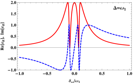
Figure 2: (Color online) The absorption $\texttt{Re}[\varepsilon_{R}]$ (red solid line) and dispersion $\texttt{Im}[\varepsilon_{R}]$ (blue dashed line) of the signal light as a function of the $\delta_{\omega}/\omega_{1}=(\delta-\omega_{1})/\omega_{1}$ while $\Delta=\omega_{1}$. The parameters used as [19], $\lambda_{l}=$1064 nm, $d=$25 mm, $\omega_{1}=\omega_{2}=2\pi\times 947\times 10^{3}$ Hz, the quality factor $Q_{1}=\frac{\omega_{1}}{\gamma_{1}}(Q_{2}=\frac{\omega_{2}}{\gamma_{2}})=6700$, $m_{1}=m_{2}=145$ ng, $\kappa=2\pi\times 215\times 10^{3}$Hz, $\wp_{l}=2$ mW, and $\lambda=8\times 10^{35}$ Hz/m².

For illustration of the numerical results, we choose the realistically reasonable parameters to demonstrate the slow and fast light effect based on the optomechanical system. We employ the parameters from the recent experiment [19] in the observation of the normal-mode splitting.

Figure 2 illustrates the behavior of the absorption $\texttt{Re}[\varepsilon_{R}(\omega_{s})]$ and dispersion $\texttt{Im}[\varepsilon_{R}(\omega_{s})]$ of the signal light as a function of $\delta_{\omega}/\omega_{1}=(\delta-\omega_{1})/\omega_{1}$. We can find obviously that there are two steep negative slopes related to two minima of zero-absorption in the reflective light. The two minima of the zero-absorption in Fig.2 can be evaluated by $\frac{d\texttt{Re}[\varepsilon_{R}(\omega_{s})]}{d\omega_{s}}\mid_{\omega_{s}=\omega_{+},\omega_{-}}=0$, where $\omega_{+}$ and $\omega_{-}$ are the points of the zero-absorption minima. This large dispersive characteristics can lead to the possibility of implementation of fast light effect. However, if we turn off the Coulomb coupling between the charged NR₁ and NR₂, the two steep negative slopes disappear and only one occurs. Which has been studied in Ref.[22].

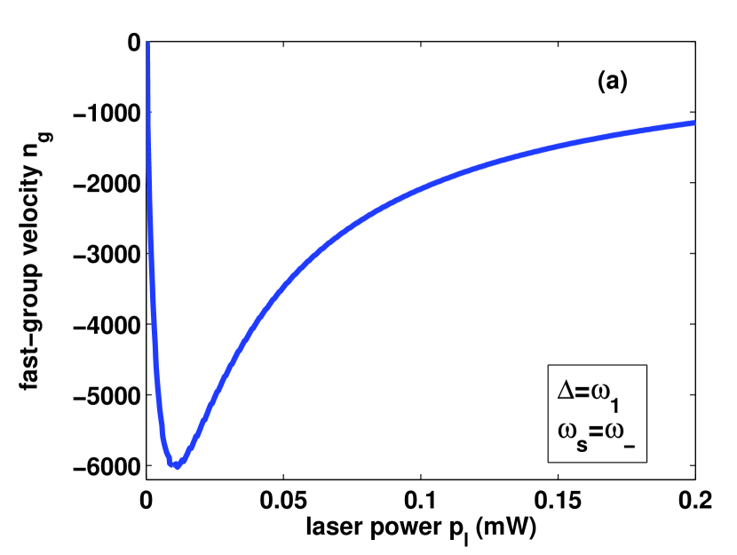
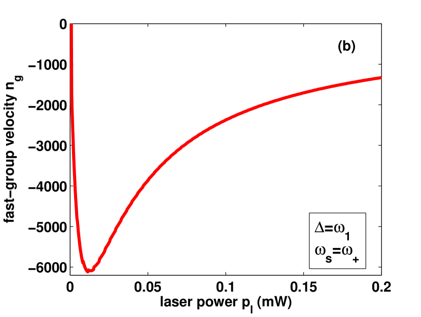
Figure 3: (Color online) The group fast velocity index $n_{g}$ as a function of the laser power $\varepsilon_{l}$ while $\Delta=\omega_{1}$, the parameters used are the same as in Fig. 2.

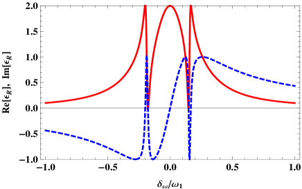
Figure 4: (Color online) The absorption $\texttt{Re}[\varepsilon_{R}]$(red solid line) and dispersion $\texttt{Im}[\varepsilon_{R}]$ (blue dashed line) of the signal light as a function of the $\delta_{\omega}/\omega_{1}=(\delta-\omega_{1})/\omega_{1}$ while Coulomb coupling strength $\lambda=2\times 8\times 10^{35}$ Hz/m². Other parameters used are the same as in Fig. 2.

Figure 3 shows the two mode group velocity $n_{g}$ as a function of the laser power and the parameters used are the same as in Fig. 2. It is clear that near $\varepsilon_{l}=0.01$mW, the fast light index can be obtained as 6000 times with two mode light frequencies $\omega_{+}$ and $\omega_{-}$ respectively. That is, the output will be 6000 times faster than the input with two different frequencies. Therefore, in our structure one can obtain the fast output light without absorption by only adjusting the effective detuning of laser field from the bare cavity equal to the frequency of the NR₁. The physics of the effects can be explained by the radiation pressure coupling an optical mode to a mechanical mode in an optomechanically induced transparency (OMIT) [18, 20]. The OMIT depends on quantum interference, which is sensitive to the phase disturbance. The Coulomb coupling between the NR₁ and NR₂ breaks down the symmetry of the OMIT interference, and thus the single OMIT window is split into two OMIT [35, 24].

Figure 4 describe the The absorption $\texttt{Re}[\varepsilon_{R}]$ and dispersion $\texttt{Im}[\varepsilon_{R}]$ of the signal light with different Coulomb coupling strength. That is to say, the frequencies of the signal light can be tuned by Coulomb coupling strength. Similarly, the optomechanical system also can implement the two mode slow light effect without absorption when the effective detuning of laser field from the bare cavity($\Delta=-\omega_{1}$). In order to illustrate it more clearly, we plot Figs. 5 and 6 with the same experimental data as in Fig. 2. In Fig. 5, we also describe the theoretical variation of absorption $\texttt{Re}[\varepsilon_{R}]$ and dispersion $\texttt{Im}[\varepsilon_{R}]$ of the signal light as a function of $\delta_{\omega}/\omega_{1}=(\delta-\omega_{1})/\omega_{1}$ when the detuning $\Delta=-\omega_{1}$. From Fig. 6 we can find that there are two the large dispersions relates to two very steep positive slopes. It means that there are two mode slow light effect without absorption. Figure 6 shows the group velocity index $n_{g}$ of two mode slow light as a function of laser power.

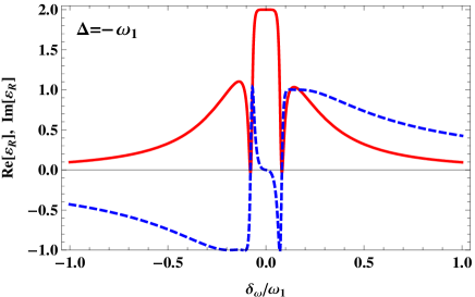
Figure 5: (Color online) The absorption $\texttt{Re}[\varepsilon_{R}]$(red solid line) and dispersion $\texttt{Im}[\varepsilon_{R}]$ (blue dashed line) of the signal light as a function of the $\delta_{\omega}/\omega_{1}=(\delta-\omega_{1})/\omega_{1}$ when $\Delta=-\omega_{1}$. Other parameters used are the same as in Fig. 2.

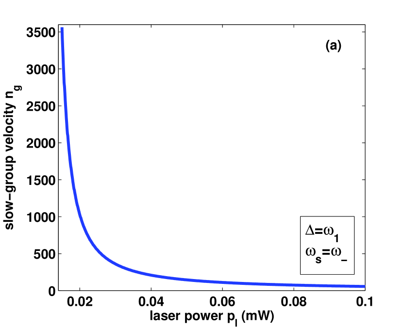
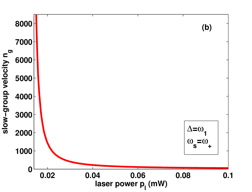
Figure 6: (Color online) The two mode slow group velocity index $n_{g}$ as a function of the laser power $\varepsilon_{l}$ when $\Delta=-\omega_{1}$. Other parameters used are the same as in Fig. 2.

According to the above discussions, it can be found clearly that the optomenchanical system provides us an efficient and two mode switch between slow light and fast light by simply adjusting the effective laser detuning in terms of the double-OMIT. In experiments, one can fix the signal field with frequency $\omega_{s}=\omega_{+},\omega_{-}$ and scan the effective laser detuning from $\Delta=-\omega_{1}$ to $\Delta=+\omega_{1}$, then one can efficiently switch the signal field from slow to fast with two different frequencies.

4 conclusions

In conclusion, we have investigated tunable fast- and slow- light effects in double mode with the optomechanical system. It can provide us an efficient and convenient way to switch between slow and fast light with double-mode. The greatest advantage of our system is that we can efficiently switch from fast to slow light by only adjusting the laser-cavity deturning. Moreover, the requencies of signal light can be tuned by Coulomb coupling strength. Our scheme may have potential applications in various applications such as optical communication, nonlinear optics.

Finally, we hope that the results of this paper can be tested by experiments in the near future. Recently, S. Weis et al.[18] and A. H. Safavi-Naeini et al.[20] have reported experimental results on signal-mode slow light and OMIT in a optomechanical system, maybe one can use a similar experimental setup to test our predicted effects.

References

References

• [1] Boyd R W and Gauthier D J 2009 Science 326 1074
• [2] Kasapi A, Jain M, Yin G Y and Harris S E 1995 Phys. Rev. Lett. 74 2447
• [3] Chu S and Wong S 1982 Phys. Rev. Lett. 48 738
• [4] Hau L V, Harris S E, Dutton Z and Behroozi C H 1999 Nature 397 594
• [5] Kash M M, Sautenkov V A, Zibrov A S, Hollberg L, Welch G R, Lukin M D, Rostovtsev Y, Fry E S and Scully M O 1999 Phys. Rev. Lett. 82 5229
• [6] Budker D, Kimball D F, Rochester S M and Yashchuk V V 1999 Phys. Rev. Lett. 83 1767
• [7] Turukhin A V, Sudarshanam V S, Shahriar M S, Musser J A, Ham B S and Hemmer P R 2001 Phys. Rev. Lett. 88 023602
• [8] Bigelow M S, Lepeshkin N N and Boyd R W 2003 Phys. Rev. Lett. 90 113903
• [9] Ku P C, Sedgwick F, Chang-Hasnain C J, Palinginis P, Li T, Wang H, Chang S W and Chuang S L 2004 Opt. Lett. 29 2291
• [10] Gigan S, B ohm H R, Paternostro M, Blaser F, Langer G, Hertzberg J B, Schwab K, Baeuerle D, Aspelmeyer M and Zeilinger A 2006 Nature (London) 444 67
• [11] Arcizet O, Cohadon P F, Briant T, Pinardand M and Heidmann A 2006 Nature (London) 444 71
• [12] Kleckner D and Bouwmeester D 2006 Nature (London) 444 75
• [13] Schliesser A, Del Haye P, Nooshi N, Vahala K J and Kippenberg T J 2006 Phys. Rev. Lett. 97 243905
• [14] Gröblacher S, Hammerer K, Vanner M R and Aspelmeyer M 2009 Nature (London) 460 724
• [15] Chan J, Chan J, Mayer Alegre T P, Safavi-Naeini A H, Hill J T, Krause A, Gröblacher S, Aspelmeyer M and Painter O 2011 Nature (London) 478 89
• [16] Dong C H, Fiore V, Kuzyk M C and Wang H L 2012 Science 338 1609
• [17] Dobrindt J M, Wilson-Rae I and Kippenberg T J 2008 Phys. Rev. Lett. 101 263602
• [18] Weis S, Rivi'ere R, Del'eglise S, Gavartin E, Arcizet O, Schliesser A and Kippenberg T J 2010 Science 330 1520
• [19] Hill J T, Safavi-Naeini A H, Chan J and Painter O 2012 Nat. Commun. 3 1196
• [20] Safavi-Naeini A H, Alegre T P M, Chan J, Eichenfield M, Winger M, Lin Q, Hill J T, Chang D and Painter O 2011 Nature (London) 472 69
• [21] Chen B, Jiang C and Zhu K D 2011 Phys. Rev. A 83 055803
• [22] Tarhan D, Huang S and Müstecaplioǧlu Ö E 2013 Phys. Rev. A 87 013824
• [23] Ma P C, Xiao Y, Yu Y F and Z M Zhang 2014 Opt. Express 22 3621
• [24] Ma P C, Zhang J Q, Xiao Y, Feng M and Zhang Z M 2014 Phys. Rev. A 90 043825 ; Wang Q, Zhang J Q, Ma P C, Yao C M and Feng M 2015 Phys. Rev.A 91 063827 Wu Q, Zhang J Q, Wu J H, Feng M and Zhang Z M 2015 Opt. Express 23 18543
• [25] Agarwal G S and Huang S 2012 Phys. Rev. A 85 021801(R)
• [26] Hensinger W K, Utami D W, Goan H S, Schwab K, Monroe C, and Milburn G J 2005 Phys. Rev. A 72 041405(R) ; Xue Z Y, Zhou J and Wang Z D 2015 Phys. Rev. A 92 022320 ; Xue Z Y, Yang L N and Zhou J 2015 Appl. Phys. Lett. 107 023102
• [27] Tian L and Zoller P 2004 Phys. Rev. Lett. 93 266403
• [28] Genes C, Vitali D, Tombesi P, Gigan S and Aspelmeyer M 2008 Phys. Rev. A 77 033804
• [29] Agarwal G S and Huang S 2010 Phys. Rev. A 81 041803
• [30] Zhang J Q, Li Y, Feng M and Xu Y 2012 Phys. Rev. A 86 053806
• [31] Walls D F and Milburn G J 1994 Quantum Optics (Springer-Verlag, Berlin)
• [32] Bennink R S, Boyd R W, Stroud C R and Wong V 2001 Phys. Rev. A 63 033804
• [33] Harris S E, Field J E and Kasapi A 1992 Phys. Rev. A 46 R29
• [34] Li J J and Zhu K D 2009 Opt. Express 17 19874
• [35] Sedlacek J A, Schwettmann A, Kubler H, Löw R, Pfau T and Shaffer J P 2012 Nature Phys. 8 819