How did a Major Confined Flare Occur in Super Solar Active Region 12192?

Abstract

We study the physical mechanism of a major X-class solar flare that occurred in the super NOAA active region (AR) 12192 using a data-driven numerical magnetohydrodynamic (MHD) modeling complemented with observations. With the evolving magnetic fields observed at the solar surface as bottom boundary input, we drive an MHD system to evolve self-consistently in correspondence with the realistic coronal evolution. During a two-day time interval, the modeled coronal field has been slowly stressed by the photospheric field evolution, which gradually created a large-scale coronal current sheet, i.e., a narrow layer with intense current, in the core of the AR. The current layer was successively enhanced until it became so thin that a tether-cutting reconnection between the sheared magnetic arcades was set in, which led to a flare. The modeled reconnecting field lines and their footpoints match well the observed hot flaring loops and the flare ribbons, respectively, suggesting that the model has successfully “reproduced” the macroscopic magnetic process of the flare. In particular, with simulation, we explained why this event is a confined eruption–the consequent of the reconnection is the shared arcade instead of a newly formed flux rope. We also found much weaker magnetic implosion effect comparing to many other X-class flares.

1. Introduction

Solar flares are sudden release of excess magnetic energy in the solar corona, a plasma environment dominated by the magnetic field (Shibata & Magara, 2011). Magnetic reconnection is believed to be the central mechanism that converts free magnetic energy into radiation, energetic particle acceleration, and kinetic energy of plasma (Forbes et al., 2006). Consequently, revealing the magnetic structures associated with reconnection and their evolution during flares is essential for understanding of the flare dynamics (Priest & Forbes, 2002).

Due to the lack of direct measurements of coronal magnetic fields, it is a prevailing way to postulate the flare magnetic evolution from the observed variations of flare plasma emission. This is because the plasma emission can reflects the geometry of the invisible magnetic field, as in most part of the corona, the plasma is “frozen” with the magnetic fields. Early studies of typical eruptive flares have converged to a standard flare model (CSHKP, Carmichael, 1964; Sturrock, 1966; Hirayama, 1974; Kopp & Pneuman, 1976), which describes the essence of flare physics. The standard model mainly concerns a magnetically bipolar source region, the simplest form of solar active regions (ARs), proposing that a twisted magnetic flux rope (corresponding to a filament) rises above the polarity inversion line (PIL), stretches the overlying closed field lines (manifested as coronal loop expansion), and produces a vertical current sheet (CS) underneath where reconnection sets in and results in two parallel chromospheric flare ribbons on both sides of the PIL. The flare ribbons are suggested as the footprints of the reconnecting field lines. They gradually move apart from one another as the reconnection goes on. Meanwhile, the ejecting flux rope eventually travels into solar wind as being a coronal mass ejection (CME), leaving behind bright flaring loops that correspond to the re-closed magnetic arcades after the reconnection. Such dynamic picture inferred from observations is usually represented by simple cartoons.

Recent observations with high spatial/time resolution and multi-wavelength imagers show that numerous solar flares are characterized by complex processes that are not present in the standard model, such as multi-stage and multi-place of filament ejections in the same event (e.g., Liu et al., 2009; Schrijver & Title, 2011; Shen et al., 2012; Romano et al., 2015), escape of homologous flux ropes (e.g., Li & Zhang, 2013), slipping motions of flare loops (e.g., Aulanier et al., 2007; Li & Zhang, 2015; Dudík et al., 2016; Gou et al., 2016), flare ribbons of unusual shapes (e.g., quasi-circular and even tri-linear shapes, Masson et al., 2009; Wang & Liu, 2012; Wang et al., 2014), multiple ribbons like remote flare ribbons distinct from the eruptive core site (or the secondary ribbon, e.g., Zhang et al., 2014), the EUV late phase after the main (impulsive) phase in certain flares (Woods et al., 2011; Dai et al., 2013; Liu et al., 2013) and etc. There are also flares without CMEs, which are usually called confined flares. Some confined flares occur with filament eruptions but failing to escape their overlying field (Ji et al., 2003; Török & Kliem, 2005; Guo et al., 2010). The others, simply without any eruption, are the most hard to interpret solely from observations, because very small changes of the coronal configuration can be detected in these flares (e.g., Jiang et al., 2012; Dalmasse et al., 2015).

To understand the mechanisms of the various complex or atypical flares requires us to characterize the realistic magnetic configurations and their evolution associated with flares. Also, from the point of view of prediction of space weather, which is heavily influenced by solar eruptions, a much more accurate understanding and reproducing of the eruption process beyond the standard or theory model is strongly required. Existing techniques to this end include static non-linear force-free field (NLFFF) reconstruction (see review papers by Wiegelmann & Sakurai, 2012; Régnier, 2013), data-constrained/driven magneto-frictional (MF) evolution method (e.g., Cheung & DeRosa, 2012; Yeates, 2014; Savcheva et al., 2015; Fisher et al., 2015), data-constrained magnetohydrodynamic (MHD) simulations (e.g., Jiang et al., 2012, 2013; Kliem et al., 2013; Amari et al., 2014; Inoue et al., 2014, 2015), and more generally, the data-driven MHD simulations (e.g., Wu et al., 2006).

Among the available techniques, the NLFFF reconstruction is used most frequently because a variety of approaches and codes for solving NLFFF have been developed within in a relatively long history (e.g., Grad & Rubin, 1958; Sakurai, 1981; Yang et al., 1986; Wu et al., 1990; Amari et al., 1997; Yan & Sakurai, 2000; He & Wang, 2006; Wiegelmann & Neukirch, 2006; Wheatland, 2006; Valori et al., 2010; Jiang & Feng, 2012), and prove to be successful for studying snapshots of the coronal fields before and after flares. Signature of flare mechanism can usually be suggested from analysis of the pre-flare magnetic fields. For example, through studying the magnetic topology, critical magnetic structures relevant to flares, such as magnetic flux rope, magnetic null points, bald patch (Titov et al., 1993), and quasi-separatrix layers (QSLs, Demoulin et al., 1996; Titov et al., 2002) could be revealed. However, analyzing the pre-flare fields cannot tell directly why and how the flares occur. The lack of dynamics is a major limitation of NLFFF reconstruction, which cannot be used for “reconstruction” of magnetic field during flares. The limitation exists similarly in the MF methods. Although in such methods, a dynamic velocity is included for making the magnetic field “evolves”, this velocity is actually pseudo since it is determined only by the Lorentz force (i.e., the veloctiy ${\mathbf{v}}={\mathbf{J}}\times{\mathbf{B}}/\nu$ where $\nu$ is the frictional coefficient) while the inertia and pressure of the plasma is neglected (Yang et al., 1986). As a result, the MF approach are still limited for the quasi-static evolution phase of the corona field. When used for modeling the magnetic field evolution, the MF method is essentially similar to the way using a time-sequence of NLFFF or MHD models reconstructed independently from a series of vector magnetogram along time to mimic the coronal evolution, although in the MF method, the magnetic fields for each time snapshot are treated to be dependent on its preceding one. It is still problematic to use the MF method to simulate the flare and eruption phase in which the plasma is in extremely dynamic evolution and often associated with magnetic reconnections, although such way has been used in analysis of evolution of flare ribbons (e.g., Savcheva et al., 2015, 2016; Janvier et al., 2016). The data-driven MHD model of Wu et al. (2006), however, just uses the line-of-sight magnetograms, and thus the non-potentiality of the coronal field cannot be fully recovered. There are models (Kliem et al., 2013; Jiang et al., 2013; Amari et al., 2014; Inoue et al., 2014) using the NLFFF reconstructed or MF calculated coronal field immediately preceding eruption (thus the unstable nature of the field has already well developed) as the initial condition for MHD simulation, which prove to be able to reproduce the fast dynamic phase of the erupting field (e.g., Jiang et al., 2013). However, these kinds of simulations do not self-consistently show how the pre-eruptive field is formed and disrupted, and thus may not be used to identify the true triggering mechanism. Also, such kind of models might not be able to reproduce confined flare, which is not likely triggered by the large-scale instability of the pre-flare magnetic field.

To self-consistently and realistically simulate the coronal evolution from its pre-flare to flare phases, we have developed a new data-driven 3D MHD AR evolution (DARE) model. The DARE model is based on the full MHD equation with its lower boundary driven directly by the solar vector magnetograms, which is unique among all the aforementioned models that attempt to simulate the realistic coronal magnetic evolution. In the first application of this model (Jiang et al., 2016), we modeled the evolution of a complex multi-polar AR with flux emergence over two days leading to an eruptive, also atypical flare. The simulation reasonably recreated the whole process from a long quasi-static evolution to the eruptive stage of extreme dynamics. It was shown that the field morphology resembles the sequence of the corresponding EUV images from SDO/AIA for such process, in addition to the successful match of the timing of the flare onset.

In this paper, we propose to use the DARE model to study a distinctly different event, a confined major X-class flare occurred in the super NOAA AR 12192 on October 2014. This AR is “super” because of its size, which is the largest of all ARs during the last 25 years. It produced a series of X-class flares without eruptions, and the strongest one in the series reaches X3.1, which sets a record in the flare energy for CMEless events (Thalmann et al., 2015) since the confined flares ever observed were predominantly below X-class (Yashiro et al., 2006). A series of studies have been inspired to explain why these extremely powerful flares did not lead to eruptions (Jing et al., 2015; Sun et al., 2015; Chen et al., 2015; Inoue et al., 2016). Here we are curious why and how did these flares occur, or more specifically, what is the evolution of the magnetic fields underlying these non-eruptive flares in AR 12192? We attempt to answer this question by simulating the coronal magnetic field evolution of the AR leading to the X3.1 flare. The rest of this paper is organized as follows. The flare event to be studied are described in Section 2. Then the DARE model is briefly presented in Section 3. Results are given in Section 4 and finally discussions in Section 5.

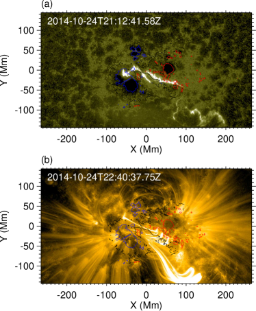
Figure 1.— Overview of the X3.1 flare occurred in AR 12192. (a) AIA 1600 Å image of the flare ribbon and (b) AIA 171 Å image of the post-flare loop. Both images are CEA re-mapped with field of view identical to that of the SHARP CEA magnetogram for this AR. Overlaid contours indicate the vertical component ($B_{z}$) of the photospheric magnetic field at the same time (red for $1000$ G, blue for $-1000$ G, and black for the PIL with the total field strength above $200$ G).

2. Event

Since overview of the AR 12192 and its unusual feature, that is, extremely large size, rich of X-class flare but CME-poor, has been described well in the literature (Thalmann et al., 2015; Sun et al., 2015; Chen et al., 2015; Jing et al., 2015; Chen et al., 2015), we focus on the X3.1 event and the relevant information with our modeling. In the period of our interest from 2014 October 23 to 24, AR 12192 is close to the central meridian. Two major sunspots are well separated by a distance of roughly $100$ Mm (see Figure 1a). The target flare occurred around 21:00 UT, October 24, and it lasts for an unusual long duration of more than one hour with the GOES X-ray flux above X class. Preceding the major flare are relatively small ones of C- and M-class with shorter durations. When inspecting the SDO/AIA images (for instance, Figure 1b) one only see a series of brightening of coronal loops without much changes in their shape. The flare loops are seen connecting the boundaries of the strong magnetic polarities. Interestingly, there is also a set of rather long loops with remote connection to the southwest corner of the field of view as shown (e.g., Sun et al., 2015; Chen et al., 2015). Chromospheric ribbons of the flare (Figure 1a) consist of mainly two bands on both sides of the central part of the PIL. Distinct from typical two-ribbon flares, these two ribbons showed barely separation motion. As such, the coronal configuration changes are not easy to interpret from these EUV observations.

3. The DARE Model

In the DARE model (Jiang et al., 2016), we used the solar surface magnetic field data from the SDO/HMI (Schou et al., 2012), in particular, the Space weather HMI Active Region Patches (SHARP) vector magnetogram data series (Hoeksema et al., 2014; Bobra et al., 2014). With the cadence of 12 min and the spatial resolution of 1 arcsec, the SHARP data are adequate to track a relatively long-term evolution (hours to days) of magnetic structures of the typical AR scale. To setup the model, we considered a local Cartesian coordinate system with its origin at the surface center of the AR, which is defined in the cylindrical equal area (CEA) re-mapped SHARP magnetogram. The 3D computational volume extends approximately $[-450,450]$ Mm in both $x$ and $y$ axes and 900 Mm in $z$ axis, which is sufficient to include the large-scale magnetic field related with the flare. Furthermore, all the external boundaries (except the bottom surface) are non-reflective. We note that here the AR spans $\sim 60^{\circ}$ of the solar sphere, much larger than typical ARs, and the curvature of the associated area should not be ignored. Thus the current modelling in Cartesian box might not appropriately characterize the geometry for the AR, and we keep in mind the possible influence in discussing our modeled results.

Based on the HMI vector magnetogram, we first constructed an approximately force-free coronal magnetic field (Jiang & Feng, 2013) corresponding to a pre-flare instance of 00:00 UT on 2014 October 23. Then, with this field as the initial condition, we numerically solved the full set of time-dependent, 3D MHD equations in the modeling volume. The bottom boundary of the model is assumed as being the coronal base, thus the magnetic field measured on the photosphere is used as a reasonable approximation of the field at the coronal base. Then the evolving solar surface magnetic fields from observation provide the time-dependent bottom boundary conditions for the simulation domain. We smoothed the original SHARP data before inputting them into the numerical model. This is necessary since the magnetic structures are broadened from the photosphere to the coronal base. We simulated such broadening using Gauss smoothing of the data with Gaussian window of $\sigma=2$ arcsec as suggested by Yamamoto & Kusano (2012). We further smoothed the data in time with Gaussian window of $\sigma=4\times 12$ min to remove short-term temporal oscillations and mitigate the problem of data spikes due to bad pixels. Interpolation in time was employed to fill small data gaps in the two days of observation.

In addition to the magnetic field, we also need to give a model of plasma in the computation. Here, the plasma is initialized in a hydrostatic, isothermal state with $T=10^{6}$ K (sound speed $c_{S}=128$ km s^-1) in solar gravity. Its density is configured to make the plasma $\beta$ as small as $2\times 10^{-3}$ (the maximal Alfvén $v_{\rm A}$ is $4$ Mm s^-1) to mimic the coronal low-$\beta$ and highly tenuous conditions. The plasma thermodynamics are simplified as an adiabatic energy equation since we focus on the evolution of the coronal magnetic field. No explicit resistivity is included in the magnetic induction equation, and magnetic reconnection is still allowed due to numerical diffusion if any CS forms and becomes thin enough with thickness close to the grid resolution (i.e., the smallest grid). A small kinematic viscosity $\nu$ is used with its value corresponding to the viscous diffusion time as $\sim 10^{2}$ of the Alfvén time in strong-field regions. This is usually necessary for the sake of numerical stability in the long term computation. The units of length and time in the model are $L=23$ Mm (approximately 32 arcsec on the Sun) and $\tau=L/c_{S}=180$ s, respectively.

Solution of the MHD equations is implemented by an advanced space-time high-accuracy scheme (AMR–CESE–MHD, Jiang et al., 2010). We use a non-uniform grid based on the magnetic flux distribution for the sake of saving computational resources. The smallest grid $\Delta x=\Delta y=\Delta z=1.4$ Mm (approximately 2 arcsec on the Sun) is made around the AR core region (approximately $[-100,100]\times[-100,100]\times[0,100]$ Mm³), where the magnetic fields are strong and evolve actively. Grid size is increased gradually to $4\Delta x$ near the side and top boundaries.

To further save the computing time, the cadence of the input HMI data into the MHD model was increased by $20$ times. By this, the model run of a realistic two-day AR evolution can be finished within about ten hours of wall time when parallelized with a medium number (for example, a hundred) of CPUs (3 GHz). Compressing of the time in HMI data is justified by the fact that the speed of photospheric flows as measured from the photospheric field evolution is about $0.1\sim 1$ km s^-1 (Welsch et al., 2004; Liu et al., 2012). So in our model settings, the evolution speed of the boundary field, even enhanced by a factor of 20, is still sufficiently small compared with the coronal Alfvén speed ($\sim$Mm s^-1 ), and the basic reaction of the coronal field to the bottom changes should not be affected. As a result, one hour in the HMI data equals one $\tau$ in the simulation. When comparing the simulation with the observations of the corona, such scaling of time (a $\tau$ equals an hour) also applies to the quasi-static evolution phase without major flares or eruptions. This is because in such phase, the coronal evolves in the same pace as the boundary, since any change in the bottom boundary is reflected almost instantly in the corona, which reaches its equilibrium very fast. But this is not justified for the dynamic phases with major eruptions or flares, in which the evolution of the corona is determined by itself rather than by the boundary. Thus, the time unit should be the original one (a $\tau$ equals $180$ s) in the flare phase.

Coupling of the coronal evolution with the continuous change of the surface magnetic field (i.e., the HMI data) is implemented by a time-dependent bottom boundary condition using the projected-characteristic method. Based on the wave-decomposition principle of the full MHD system (Nakagawa et al., 1987; Wu et al., 2006), the method can naturally mimic the transferring of magnetic energy and helicity to the corona from below (Wu et al., 2006) by self-consistently calculating the surface flow field (Wang et al., 2008), which otherwise would have to be derived by local correlation tracking or similar techniques (Welsch et al., 2004; Schuck, 2008). As in our settings, the cadence of HMI data is $\tau/5=36$ s. However, the time step in the numerical model is set as $\Delta t={\rm CFL}\min(\Delta x/v_{\rm A})=0.2$ s according to the Courant–Friedrichs–Lewy (CFL) stability condition (Courant et al., 1967) with a CFL number of 0.5. We thus linearly interpolate the HMI data in time to produce a data set with cadence matching the time step of the MHD model.

We followed the evolution of the MHD system for two days from 00:00 UT of October 23 ($t=0$) to 00:00 UT of October 25 ($t=48$).

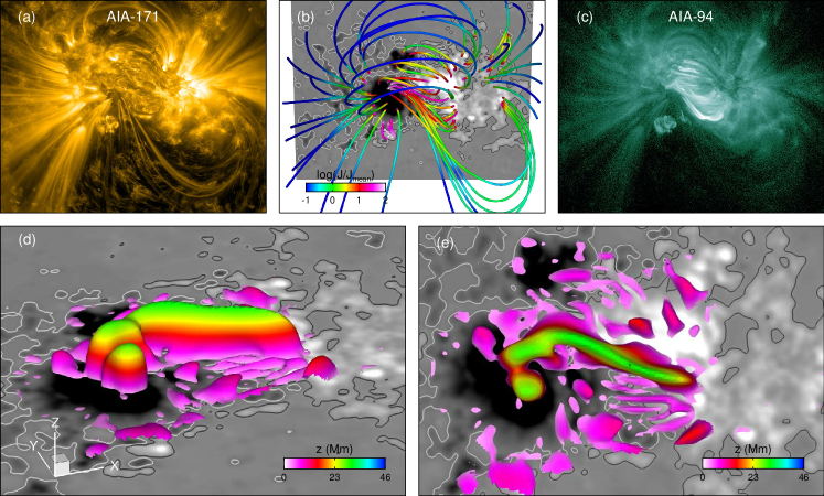
Figure 2.— AIA images and the simulated magnetic configuration of AR 12192 at 00:00 UT of 2014 October 23 (i.e., simulation time $t=0$). (a) AIA 171 Å image. (b) Selected magnetic field lines of the MHD simulations. The background shows map of the photospheric $B_{z}$ (saturated at $\pm 1000$ G). Contour lines (black and white) are also shown for $\pm 100$ G. The color of the plotted field lines denotes the strength of the associated electric current density $J$ (scaled by the mean value $J_{\rm mean}$ of the entire model volume). (c) AIA 94 Å image. (d) The side view of the volume with the current density higher than 20 times the mean value. The color denotes the height $z$ from the bottom boundary. (e) The top view of the same current volume shown in (c). Contour lines (black and white) are also shown for $\pm 100$ G.

4. Results

4.1. The initial state

In Figure 2 we show the magnetic configuration derived from the near force-free model for the initial state ($t=0$) of the MHD simulation. On the large scales, the AR exhibits a bi-polar magnetic configuration consisting of two main sunspots with a relatively strong-sheared core fields embedded in a less-sheared envelope fields. The core fields carry relatively much stronger electric current (e.g., current density higher than 20 times of the average value of the whole model box, see Figure 2b, d and e) that is concentrated within a narrow vertical layer roughly along the central part of the PIL separating the two major polarities. Such an association of intense current layer with PIL of AR core might be common for flare-productive ARs (e.g., Sun et al., 2015). Here the current layer extends from the bottom to a relatively large height ($\sim 35$ Mm, see Figure 2d). From a visual comparison with the EUV images (Figure 2a, b and c), the simulated magnetic field lines show good agreement with the observed coronal loops. In particular, it can be seen that the weakly sheared envelope fields resemble the long cool loops imaged in the AIA 171 Å channel (about 1 MK), and the strongly sheared core fields resemble the short hot loops imaged in the AIA 94 Å channel (about 6 MK). This is likely due to heating by dissipation of the strong current in the core region, making the plasma there hotter than the surroundings. In the following we show how this coronal field evolved when driven by the photospheric magnetic evolution.

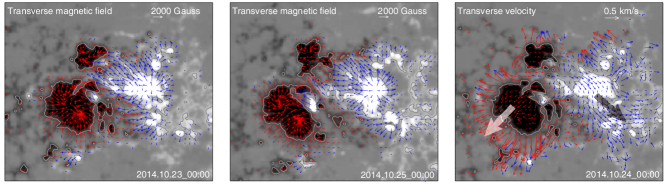
Figure 3.— Left and middle panels are SDO/HMI vector magnetograms (left and middle) for AR 12192 recorded at two different times. The vertical component $B_{z}$ as shown saturated at $\pm 1000$ G. Right panel are photospheric horizontal velocity derived using the DAVE4VM code, overlaid on the $B_{z}$ map. The two big arrows illustrate the large-scale movement of the magnetic polarities. See also animation of the evolution of the vector magnetograms during two days of interest.

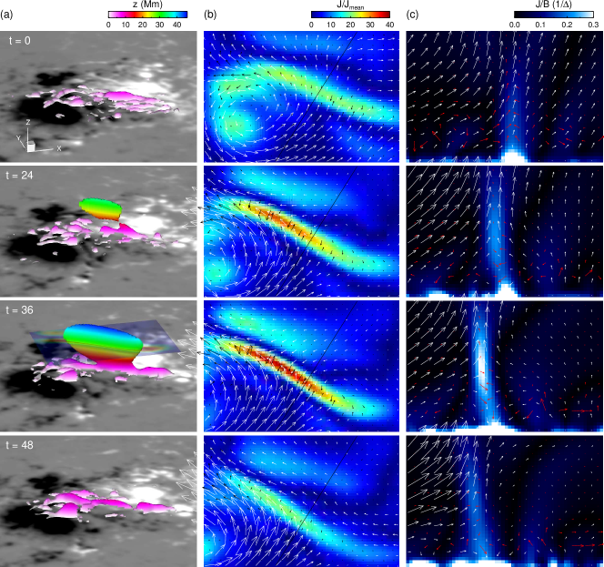
Figure 4.— Evolution of the electric current in the MHD model. (a) 3D shape of the CS (defined in the text) at four different times from the beginning to the end of the simulation. The color denotes the height from the bottom surface, which is shown by the photospheric $B_{z}$ map. (b) A horizontal slice of the volume at $z=28$ Mm. Its position is indicated by the transparent image shown in $t=36$ of (a). The color shows electric current density $J$ (scaled by the average value $J_{\rm mean}$ at $t=0$), and the arrows show plasma velocity vectors (white arrows) as well as Lorentz force vector (black arrows). The time is the same as (a) from top to bottom. (c) A vertical slice whose horizontal location is denoted by the black inclined line in (b). Vertically, it extends from the bottom to $z=57$ Mm. The color shows the value of $J/B$ and the arrows represent the velocity (white) and Lorentz force (red). Note that in (b) and (c) each pixel represents a computational grid. An animation for the 3D CS evolution and a horizontal slice is provided, in which the time step is $\tau/5$.

Figure 5.— Temporal evolution of different parameters (defined in the text) associated with the CS. (a) The intensity of the CS. (b) Rate of magnetic energy injection into the CS. (c) Total magnetic energy injected into the CS with time. (d) Total magnetic energy reserved in the CS volume. The dashed line denotes $t=30$.

4.2. Dynamic evolution

Figure 3 and its supplementary animation show how the photospheric magnetic field evolved over the two day time period. Continuous movements of the polarities can be seen, which could stress the coronal field. For instance, a horizontal flow map derived for the time moment of 00:00 UT on 2014 October 24 using the DAVE4VM method (Schuck, 2008) demonstrates clearly a diverging motion of the two main sunspots. Driven by the magnetic field evolution at the bottom, the MHD system continuously evolved in response. The basic configuration of the coronal field shows no significant changes when we trace the magnetic field lines (thus not shown in the figures here), and the total kinetic energy maintains in a rather low level (less than 0.5 percent of the total magnetic energy) without significant variation in the whole time interval, indicating that no eruption occurs in the simulation. However, evolution of the distribution of electric current, particularly the CS, a thin layer of intense current as defined below, provides instructive information that might be associated with the flare processes.

Here we use a way following Gibson & Fan (2006) to locate the CS. It is defined as the volume in which the ratio of the current density to the magnetic field strength, i.e., $J/B$, is greater than $C/\Delta x$, where $\Delta x$ is the local grid size and the constant number $C\sim 1$. Such a definition is reasonable because $J/B\sim(\Delta B/B)/\Delta x$, where $\Delta B$ denotes the gradient of magnetic field vectors in adjacent grid points, and $\Delta B/B<<1$ in the smooth region of magnetic field (except regions with $B\sim 0$, for example, near magnetic null points). While a large value of $\Delta B/B\sim 1$ indicates significant change of magnetic field (as large as the local field strength) between adjacent grid points. This means that the magnetic field vectors of distinctly different directions are squeezed extremely close to each other, forming a narrow interface with strong current, which is a CS in the context of our numerical model. When the gradient of magnetic field vectors across the CS is steepened sufficiently, numerical diffusion will take effect and “reconnection” could occur in the MHD model. In other words, for such case, the inversely-directed magnetic components on both sides of the CS are brought so close to each other that they “merge” within the CS, resulting in new connections of the corresponding magnetic field lines, and thus related to topological changes of the field. By inspecting the value of $J/B$, we find a suitable value of $C=0.2$ which can well exclude the region of weak current, and such definition gives the width of the CS of $\sim 3\Delta x$. It should be noted here the CS is different from that in theoretical view, i.e., an infinitely thin or simply a 2D surface rather than a finite volume.

The 3D shapes of the CS at different times are shown in Figure 4a (and also in its supplementary animation). A horizontal slice of the volume is shown in Figure 4b, and a vertical slice in Figure 4c. Initially ($t=0$) the CS did not yet form, thus there are only small-scale structures near the bottom surface. Then, successive formation, expansion and shrinkage of the CS volume are seen. From the plasma flows and the Lorentz force vectors around the CS volume, we can see that the initial current layer is gradually squeezed from both two sides by the magnetic stress. Consequently it becomes thinner and more intense, leading to increasing of the value $J/B$ and thus the formation of the CS as we defined ($J/B>0.2\Delta x$). At the time of $t=36$ (close to the peak stage of the CS development, see below), the CS extends from the bottom of the simulated domain up to heights of 50 Mm. With the slow evolution of the basic configuration, the CS also moves slowly from north to south, but overall its location is roughly the same in whole period. Interestingly, the pattern of reconnection-like plasma flow, i.e., horizontal inflow at both sides of the CS and vertical outflow to up and down, can be seen (Figure 4b and c, see $t=24$ and $36$, for example), suggesting that reconnection might occur in the simulation.

We then calculated the following parameters to characterize the CS evolution and to see whether reconnection occurred within the CS:

1. Since in the evolution process the CS grows and decays dynamically, for each time snapshot, we integrate $J/B$ for the full volume $V$ of the CS as defined above, which gives a value $I_{\rm CS}=\int J/BdV$ in unit of area, and can be used to quantify the size or intensity of the evolving CS;

2. Furthermore, we calculated the rate of the magnetic energy injection into the CS by $F_{\rm CS}=-\int_{S}{\mathbf{P}}dS=-\int_{V}\nabla\cdot{\mathbf{P}}dV$, where ${\mathbf{P}}=\frac{1}{4\pi}{\mathbf{B}}\times({\mathbf{v}}\times{\mathbf{B}})$ is the Poynting flux vector with ${\mathbf{v}}$ as the plasma velocity, and $S$ is the surface area of the CS volume $V$;

3. The total magnetic energy injected into the CS, i.e., $E_{F}=\int_{0}^{t}F_{\rm CS}dt$ at time $t$;

4. As here the CS is not a 2D surface but has a finite volume, we would like to know the magnetic energy ($E_{\rm CS}=\int_{V}\frac{B^{2}}{8\pi}dV$) in the CS volume. So the happening of reconnection can be indicated if the magnetic energy stored in this volume is less than those injected into it.

The results are shown in Figure 5. If omitting the small fluctuations of the CS size profile during the whole process, we find that its evolution consists of two phases of distinct behaviors: in the first phase from $t=0$ to approximately $30$, it keeps a relatively small value ($\sim 200$ Mm²); in the second phase from $t=30$ to the end of the simulation, it first increases impulsively and reaches the peak value of 1600 Mm² at nearly $t=40$, and then decreases rapidly to a value similar to that in the first phase. The evolution of the rate of magnetic energy injected into the CS, $F_{\rm CS}$, shows a similar trend. In the later phase (i.e., from $t=30$ to the end), the total magnetic energy input is about $10^{33}$ erg, while the magnetic energy in the CS volume is smaller by nearly two orders in magnitude and can be negligible. This indicates that the amount of the magnetic energy injected into the CS is mostly released via reconnection (converted into other forms), and the energy release rate can be approximated by $F_{\rm CS}$. If we regard the impulsive increase and decrease of the energy release rate in the CS as a simulated “flare” process, we estimate the released energy by the flare is about $10^{33}$ erg and the energy conversion rate is on the order of $10^{29}$ erg s^-1, and can reach an order higher in the peak time. For a reference, the potential energy of this AR is approximately $1.5\times 10^{34}$ erg during our studied period, over an order higher than typical-size ARs, e.g., AR 11158 (Sun et al., 2015). On the other hand, the first phase ($t=0$ to $30$) can be regarded as a quasi-static evolution duration for which the time unit $\tau$ can be scaled as being one hour, as mentioned in Section 3. This means that our simulated flare ($t=30$) began $15$ hours ahead of the real X3.1 flare ($t\sim 45$). However, for the simulated flare phase, the time duration of nearly 20 $\tau$, and thus equaling one hour (since $\tau=180$ s), is close to the real one that has relatively long X-ray duration of about one hour.

The above analysis of the CS evolution based on the modeled results suggests a reasonable picture of how the real flare was produced: photospheric field evolution stressed the coronal field and built up a large-scale CS in the core region, then magnetic reconnection was triggered immediately and resulted in impulsive release of magnetic energy. As the kinetic energy is very low even during the impulsive phase of energy release, the most of the released magnetic energy should be converted into energy of accelerated electrons (ions also possible), and subsequently in the form of radiation at various wavelengths. However, our simulation cannot reproduce this process because we did not include the related physics in the model. Nevertheless, the modeled results are in an agreement with the fact that this was a non-eruptive flare, during which no significant disruption of the coronal field was observed.

It is worthy noting that there were small fluctuations, i.e., short episodes of relatively small-scale CS formation and dissipation before the major one. These fluctuations reflect the energy build up and might be the simulation counterparts of the small flares that occurred before the main one (but a one-to-one correspondence was not reproduced). In fact, it signifies that the magnetic field is stressed and from time to time and the process is interrupted by episodic small-scale reconnection. However, preceding to the major flare, the CS is not large enough for the global-scale reconnection to set in.

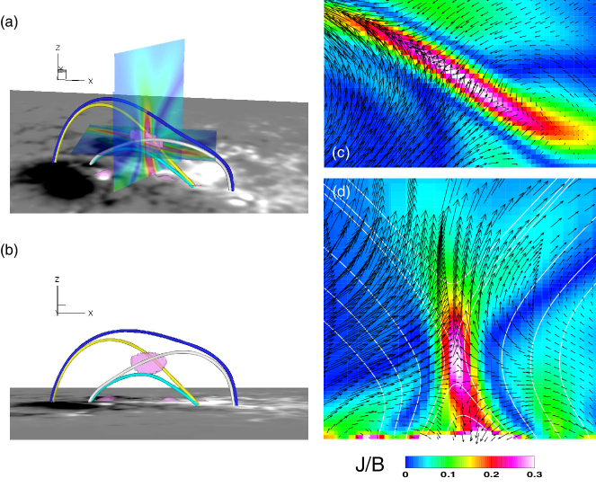
Figure 6.— Illustration of the tether-cutting reconnection process in the model. (a) Sampled field lines and horizontal and vertical cross sections of the reconnection site. The white and yellow curves represent the “before” flare field lines and blue and cyan curves show the new reconnected field lines. The pink colored area shows the iso-surface of $J/B=0.3/\Delta x$, which is sandwiched between the pre-reconnection field lines at their crossing point. (b) Side view of the sampled field lines. (c) and (d) The horizontal and vertical cross sections zoomed-in to show details of the $J/B$ (in unit of $1/\Delta x$) structures and plasma flow vectors. The vertical axis of in (c) is $z$ in range of $[0,92]$ Mm. The white curves in (c) are 2D field projections of the field lines mapped on the slice.

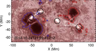
Figure 7.— AIA 1700 Å image of the flare ribbon at the beginning of the flare. Four initial brightening flare patches are marked by circles. The contour lines represent photospheric $B_{z}$ of $\pm 1000$ G.

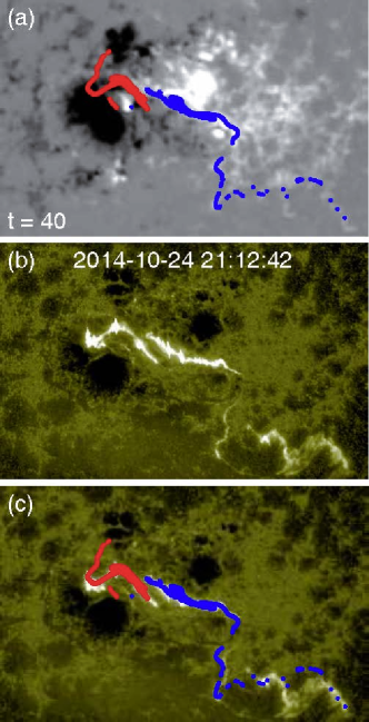
Figure 8.— Comparison of the footpoints of reconnecting field lines in the model with the observed flare ribbons. (a) The modeled footpoints overlaid on photospheric magnetogram of $B_{z}$ (saturated at $\pm 1000$ G). Results are produced at the modeling time $t=40$, when the CS size attained the peak value. Footpoints in positive (negative) magnetic flux are shown with blue (red) color. (b) AIA 1600 Å image of the chromospheric flare ribbons. The image is re-mapped and co-aligned with the magnetogram shown in (a). (c) The modeled footpoints overplotted on the AIA image.

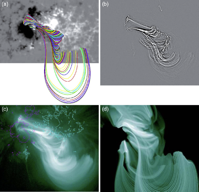
Figure 9.— Comparison of the reconnecting field lines from the model with the observed flaring loops. (a) The reconnecting field lines (modeling time at $t=40$). They are shown with different colors for better discrimination of each field lines. (b) High-pass filtered AIA 94 Å image highlighting the flaring hot loops. (c) Original AIA 94 Å image. Overlaid contours represent photospheric $B_{z}$ of $\pm 1000$ G. (d) A Synthetic EUV image of the flaring loops based on the modeled magnetic field and currents (specified in the text).

4.3. Reconnection configuration and comparison with observations

In Figure 6a and b we trace sampled field lines to illustrate the reconnection configuration. These four field lines are selected from the model at the peak time $t=40$ of reconnection. The yellow and white lines are traced from the core site of the CS (shown by the pink object) and they represent the pre-reconnection field lines. These field lines (yellow and white) are sheared and pass each other at their inner footpoints, while the CS was formed at the interface between the crossing field lines. These field lines later reconnected and changed their connectivity forming a longer field line (blue) connecting the two outer-most footpoints and a shorter line (cyan) connecting the two inner footpoints. By the magnetic tension force, both the post-reconnection field lines relax. The longer field line expands upward but only slightly, and the shorter line contracts downward. Further evidence of this type of reconnection are the plasma inflows and outflows associated with the CS (i.e., diffusive region), horizontal and vertical slices of which made near the reconnection point are shown, in Figure 6c and d. Although the reconnection configuration are of full 3D, shown in the vertical slice they exhibits a typical X-shaped two-dimensional (2D) reconnection picture. Thus locally such reconnection can be considered in a 2D framework with a strong guide field (i.e., out-of-the-plane component).

To support the association of the modeled reconnection configuration with the real flare event, observed signatures of the flare emission can be compared with the modeled results, in an indirect way. Among these are the location and shape of the chromospheric flare ribbons, which are recognized to be an indicator of the footpoint locations of those magnetic field lines that underwent reconnection (Qiu, 2009). This is mainly due to the non-thermal particles accelerated at the reconnection site traveling down along these field lines toward the photosphere and colliding with the dense chromosphere causing enhanced heating (Reid et al., 2012).

As the sampled field lines shown in Figure 6 are traced from the core site of the CS (where $J/B$ is the strongest), they can be regarded as the “first” field lines that reconnect in the whole simulated flare process (however, it is difficult to precisely locate the first reconnection point and field lines in the model). These first reconnected field lines have four footpoints at the bottom, and each of them, from left to right as shown in Figure 6a, roughly corresponding to the four brightening patches as shown in Figure 7, from left to right, respectively, which are identified in AIA 1700 Å channel at the flare beginning. Both the simulation and the observation show that the two inner flaring points are separated by a relatively large distance of approximately $50$ Mm. The simulation also suggests that the initial reconnection point is already rather high ($\sim 30$ Mm) in the corona.

Following the initial reconnection, the reconnection site should extends horizontally and forms a line of reconnection points with similar X-shaped configuration at their vertical slice. Along the central line of the CS (see the regions with $J/B>0.3/\Delta x$ shown in Figure 6c), we can see the horizontal reconnection inflow vectors are almost perpendicular to the CS. This central line is a hint of such reconnection line. When all the field lines along the reconnection line are involved in, the two ribbons form (see Figure 8b). To simulate such ribbons, we identify all the reconnecting field lines as those that are in contact or pass through the CS (see Figure 9a), which means that these field lines were undergoing reconnection or formed immediately after reconnection. The footpoints of these field lines, when mapped on the photosphere, appear to form two curved narrow areas separated by the central PIL (Figure 8a). A strikingly good match in both the location and the shape of these simulated footpoint areas with the observed chromospheric flare ribbons is evident (Figure 8b and c), including even the relatively weak ribbon extending far in the southwest direction.

The flaring loop in the hot channels (e.g., AIA-94) can also be compared with our simulated field (see Figure 9a and b). For a better vision comparison, we generated a synthetic EUV image using a method similar to that used by Cheung & DeRosa (2012). We first trace a large number ($3\times 10^{5}$) of field lines from their footpoints uniformly distributed at the bottom. Then we assign for each field line a value of emission assumed to be $J/BJ^{2}$ at the peak value point of $J/B$ along the field line. Here $J/B$ can be regarded as the dissipation rate of current, and by selecting its maximum, we can emphasize the emission from the reconnecting field lines. Finally the total emission is obtained by integration through the volume along the line-of-sight (here simply along the $z$-axis), and forms the synthetic image. As shown in Figure 9c and d, a good morphological similarity is achieved between the simulated emission and the AIA-94 images of the hot flaring loops.

As can be seen from the comparison, the ribbons in the core region correspond to the footpoints of the short field lines there, which reveal themselves as the short contracting loops. The far southwest ribbon is due to the long field lines that connect the negative-polarity sunspot and the far southwest plage region next to the positive-polarity sunspot, and these long field lines correspond to the long flaring loops. This might explains why flares frequently involve the brightening of these long side loops. We note that the shape of long loops appear not to be very well reproduced. This is possibly because they are close to the side boundaries of the simulation volume and thus the modeling of the field there is subject to the influence of the numerical boundary conditions, especially during such a long-term computation. A more important factor could be that our model is based on Cartesian geometry, thus failed to accurately reproduce the very long loops for which the curvature of the Sun must be considered. Nonetheless, the mapping of the field lines to the bottom surface is still accurate.

5. Discussions

We simulated the magnetic dynamics of AR 12192 in a two-day period using the DARE model with the SDO/HMI vector magnetograms as evolving boundary input. Analysis of the modeled results shows that a large-scale CS is developed in the AR core field due to stressing by photospheric driving, and then reconnection is triggered within the CS, resulting in an impulsive release of magnetic energy, which could correspond to an X3.1 flare occurred near the end of the period. The reconnection configuration exhibits signatures of the tether-cutting reconnection (Moore et al., 2001). Comparison with the AIA observations shows that the model almost reproduced exactly the location of the chromospheric flare ribbons, and the morphology of the reconnecting field lines and the simulated EUV image resembles well the flaring coronal loops. Such an agreement of simulation with observations supports that our model correctly captured the essentials of the MHD process of this flare. Observations (Chen et al., 2015) show that the X-flares in the same AR exhibited very similar flaring structures, indicating that these flares were homologous flares with analogous magnetic mechanism. This might indicate multiple recurrence of the process from slow formation to fast dissipation of the intensive current layer between the sheared arcades, while the large-scale configuration of the AR does not change much.

Analysis of the magnetic decay index (Sun et al., 2015; Inoue et al., 2016; Jing et al., 2015) seems to explain why the flare failed to erupt, as the overlying closed magnetic field is sufficiently strong to confine the eruption from below (see another failed eruption shown in Wang et al., 2015). Here the DARE simulation provides additional and direct explanations. As can be seen from a direct look of the field lines (see Figure 6), the pre-flare magnetic arcades are twisted (or stressed) by a rather weak extent. A quantitative study of the magnetic twist has been performed by Inoue et al. (2016) for the same flare event using a NLFFF model. They found that the magnetic twists before the flare is mostly less than a half turn. Consequently, the sheared magnetic arcades do not show a well-formed two-J shape like those in many sigmoid ARs with eruptive events. Inoue et al. (2016) also showed that after the flare, the magnetic twists are almost reserved without release. This is consistent with our modeled results that the post-reconnection field lines are still sheared arcades, without forming an escaping magnetic flux rope. In our simulation, the reconnected long field lines on top of the CS only expands slightly without propagating further to make the overlying arcades open. Thus, in the context of tether-cutting scenario, only the first-stage of tether-cutting occurred, while the second stage, formation of a flux rope and reconnection below the flux rope, did not happen.

Another unusual fact of this flare is that the enhancements of the horizontal field at the photosphere is very weak (Sun et al., 2015). This is unlike in many other large flares, as an evident enhancement of photospheric horizontal field after flare is commonly observed (Wang, 2006; Wang & Liu, 2010; Wang et al., 2012; Petrie, 2012). In the proposed coronal “implosion” mechanism (Hudson, 2000), such enhancement of photospheric field is due to the downward contraction of the short magnetic arcades formed after the reconnection and their push on the photosphere. As we found in the simulation here, the reconnection site is rather high above the photosphere, which is also suggested by Thalmann et al. (2015) from the study of the limited variation of the flare-ribbon separations. As a result, the reconnected short field lines below the CS expanded still rather highly in the corona. So during its contraction, the effect of its push on the bottom might be reduced significantly by the strong corona field below. Thus the large altitude of the reconnection sites and the long extension of the reconnected arcades provide a plausible explanation for the weak “implosion” effect. A further quantitative analysis of this effect will be considered in future works.

It has been found that the magnetic energies from NLFFF models usually underestimate the related flare energies (e.g., Sun et al., 2012; Feng et al., 2013). For the present X3.1 flare, Sun et al. (2015) gives a result of $0.9\times 10^{32}$ erg from a NLFFF extrapolation code. As a reference, Thalmann et al. (2015) estimated that the non-thermal electron energy for an earlier, confined X1 flare as $1.6\times 10^{32}$ erg, so the X3.1 flare energy is likely to be much larger than this value. On the other hand, from our simulation we have estimated a total released magnetic energy of $10^{33}$ erg, which is an order higher than that derived from the NLFFF model (Sun et al., 2015) and appears to be sufficient for powering the X3.1 flare. Such an unusually large value of energy release (compared with typical ARs) is still reasonable when considering the unusually large size of this AR with potential energy of about $1.5\times 10^{34}$, a order higher than typical ARs. While the NLFFF model calculates the drop of total magnetic energy of the whole modeling volume from pre-flare to post-flare states, we can directly calculate the magnetic energy lost in the CS due to the “reconnection” within the CS, which should be more relevant with the flare-released energy. As such, we did not perform energy analysis for the full modeling volume.

Recently, Savcheva et al. (2015) claimed that based on MF or NLFFF models and searching of QSLs, they were able to predict the locations of the flare ribbon. However, we note that the QSLs are only possible sites for reconnection, while they cannot tell where the reconnection occurs specifically in a flare. Moreover, by inspecting the map of QSLs, one usually see much more complex structures than that of target flare ribbons (see Figure 5 in Savcheva et al. (2015)). Thus without knowing ribbon locations in advance, it is still problematic to identify from all the QSLs the particular flare-related one. Here with the MHD model we simulated the flare reconnection process in a self-consistent way and directly identified the reconnecting field lines, and thus we are able to almost reproduce precisely the flare ribbon locations.

We find that the modeled “flare” began (at $t\approx 30$) well before the photospheric magnetic field input at the bottom boundary evolving to the time of the real flare (at $t\approx 45$). A perfect model of reproducing the reality should produce a flare at the exact time when the photospheric field reaches the flare onset time. The mismatch of our model with the reality is probably in a large part due to the over-simplification of the magnetic reconnection process, which might be much more complex since it is related to the microscopic behavior of plasma. However, as in many other solar MHD codes, the modeled reconnection here is simply resulted by numerical viscosity in the CS region, and its behavior depends on the numerical aspects of the model. For example, the thickness of the modeled CS and the numerical viscosity are often sensitive to the grid resolution (as well as the specific numerical scheme). A much thinner CS can develop if using a smaller grid size, and the onset of reconnection in the CS might be postponed. Namely, with a smaller grid size, a CS can sustain even stronger current and thus even larger gradient of magnetic field, which might needs more time to form. Further experiments using different grid resolutions will be required to quantify this effect.

Comparative study of this flare with eruptive ones may provide insight in the different magnetic natures of eruptive and confined flares. Here we refer to our previous study in which we use the DARE model to simulate an eruption event in AR 11283 (Jiang et al., 2016). For that event, the eruption onset time is matched by the model much better, with less than a time lag of $2\tau$ during a whole simulated period of $60\tau$. Unlike this event, the simulated eruption in AR 11283 is due to the formation of a jet-like magnetic configuration that favors breakout-like reconnection (Antiochos et al., 1999). So in that event, the critical condition causing eruption is the formation of a reconnection-favorable magnetic topology, which can be regarded as a macroscopic behavior. Whereas in AR 12192, cause of its flare depends more on the triggering of the reconnection rather than the formation of a favorable topology, since the basic topology is simply a configuration of sheared arcades and it does not change for days. In other words, the cause of the flare relies more on the microscopic behavior of the plasma and thus is more subtle. The MHD model seems to be able to characterize well the macroscopic structures and evolutions, while it may not appropriately simulate the microscopic aspects of the plasma, and thus, the triggering of the reconnection. Such difference might be common and even fundamental between eruptive flares and confined flares, in particular, those events without noticeable changes of the coronal structures.

Finally, the reconnection-related quantities derived from the model should be taken with cautions because of the simplification of reconnection. A deeper understanding of the flare dynamics requires knowledge of the true nature of magnetic reconnection and is beyond the scope of this paper. In addition, the quantitative results suffered uncertainties from several aspects including HMI data and model settings. For example, the evolution speed of the photospheric magnetic field is increased in the model for saving computing time, and this might affect the coronal evolution, most likely at the time around the flare.

In summary, the present data-driven simulation study can provide important insight in understanding why and how solar flares occur, particularly, for those events in which the dynamic change is elusive in observations. Further advancements, including more realistic plasma model, reconnection realization and thermodynamics as well as extension to spherical geometry, are necessary for even more sophisticated modeling of real solar flares. With these improvements, the DARE model will hopefully become a useful tool to the communities of solar physics and space weather.

References

- Amari et al. (1997) Amari, T., Aly, J. J., Luciani, J. F., Boulmezaoud, T. Z., & Mikic, Z. 1997, Sol. Phys., 174, 129
- Amari et al. (2014) Amari, T., Canou, A., & Aly, J. J. 2014, Nature, 514, 465
- Antiochos et al. (1999) Antiochos, S. K., DeVore, C. R., & Klimchuk, J. A. 1999, ApJ, 510, 485
- Aulanier et al. (2007) Aulanier, G., Golub, L., DeLuca, E. E., Cirtain, J. W., Kano, R., Lundquist, L. L., Narukage, N., Sakao, T., & Weber, M. A. 2007, Science, 318, 1588
- Bobra et al. (2014) Bobra, M. G., Sun, X., Hoeksema, J. T., Turmon, M., Liu, Y., Hayashi, K., Barnes, G., & Leka, K. D. 2014, Sol. Phys., 289, 3549
- Carmichael (1964) Carmichael, H. 1964, NASA Special Publication, 50, 451
- Chen et al. (2015) Chen, H., Zhang, J., Ma, S., Yang, S., Li, L., Huang, X., & Xiao, J. 2015, ApJ, 808, L24
- Cheung & DeRosa (2012) Cheung, M. C. M. & DeRosa, M. L. 2012, ApJ, 757, 147
- Courant et al. (1967) Courant, R., Friedrichs, K., & Lewy, H. 1967, IBM journal of Research and Development, 11, 215
- Dai et al. (2013) Dai, Y., Ding, M. D., & Guo, Y. 2013, ApJ, 773, L21
- Dalmasse et al. (2015) Dalmasse, K., Chandra, R., Schmieder, B., & Aulanier, G. 2015, A&A, 574, A37
- Demoulin et al. (1996) Demoulin, P., Henoux, J. C., Priest, E. R., & Mandrini, C. H. 1996, A&A, 308, 643
- Dudík et al. (2016) Dudík, J., Polito, V., Janvier, M., Mulay, S. M., Karlickỳ, M., Aulanier, G., Del Zanna, G., Dzifčáková, E., Mason, H. E., & Schmieder, B. 2016, The Astrophysical Journal, 823, 41
- Feng et al. (2013) Feng, L., Wiegelmann, T., Su, Y., Inhester, B., Li, Y. P., Sun, X. D., & Gan, W. Q. 2013, ApJ, 765, 37
- Fisher et al. (2015) Fisher, G. H., Abbett, W. P., Bercik, D. J., Kazachenko, M. D., Lynch, B. J., Welsch, B. T., Hoeksema, J. T., Hayashi, K., Liu, Y., Norton, A. A., Dalda, A. S., Sun, X., DeRosa, M. L., & Cheung, M. C. M. 2015, Space Weather, 13, 369, 2015SW001191
- Forbes et al. (2006) Forbes, T. G., Linker, J. A., Chen, J., Cid, C., Kóta, J., Lee, M. A., Mann, G., Mikić, Z., Potgieter, M. S., Schmidt, J. M., Siscoe, G. L., Vainio, R., Antiochos, S. K., & Riley, P. 2006, Space Sci. Rev., 123, 251
- Gibson & Fan (2006) Gibson, S. E. & Fan, Y. 2006, J. Geophys. Res., 111, A12103
- Gou et al. (2016) Gou, T., Liu, R., Wang, Y., Liu, K., Zhuang, B., Chen, J., Zhang, Q., & Liu, J. 2016, The Astrophysical Journal Letters, 821, L28
- Grad & Rubin (1958) Grad, H. & Rubin, H. 1958, in 2nd Int. Conf. Peac. Uses of Atom. Energy, Vol. 31, 386
- Guo et al. (2010) Guo, Y., Ding, M. D., Schmieder, B., Li, H., Török, T., & Wiegelmann, T. 2010, ApJ, 725, L38
- He & Wang (2006) He, H. & Wang, H. 2006, MNRAS, 369, 207
- Hirayama (1974) Hirayama, T. 1974, Sol. Phys., 34, 323
- Hoeksema et al. (2014) Hoeksema, J. T., Liu, Y., Hayashi, K., Sun, X., Schou, J., Couvidat, S., Norton, A., Bobra, M., Centeno, R., Leka, K. D., Barnes, G., & Turmon, M. 2014, Sol. Phys., 289, 3483
- Hudson (2000) Hudson, H. S. 2000, The Astrophysical Journal Letters, 531, L75
- Inoue et al. (2016) Inoue, S., Hayashi, K., & Kusano, K. 2016, ApJ, 818, 168
- Inoue et al. (2014) Inoue, S., Hayashi, K., Magara, T., Choe, G. S., & Park, Y. D. 2014, The Astrophysical Journal, 788, 182
- Inoue et al. (2015) —. 2015, The Astrophysical Journal, 803, 73
- Janvier et al. (2016) Janvier, M., Savcheva, A., Pariat, E., Tassev, S., Millholland, S., Bommier, V., McCauley, P., McKillop, S., & Dougan, F. 2016, arXiv preprint arXiv:1604.07241
- Ji et al. (2003) Ji, H., Wang, H., Schmahl, E. J., Moon, Y.-J., & Jiang, Y. 2003, ApJ, 595, L135
- Jiang & Feng (2013) Jiang, C. & Feng, X. 2013, ApJ, 769, 144
- Jiang et al. (2012) Jiang, C., Feng, X., Wu, S. T., & Hu, Q. 2012, ApJ, 759, 85
- Jiang & Feng (2012) Jiang, C. W. & Feng, X. S. 2012, ApJ, 749, 135
- Jiang et al. (2013) Jiang, C. W., Feng, X. S., Wu, S. T., & Hu, Q. 2013, ApJ, 771, L30
- Jiang et al. (2010) Jiang, C. W., Feng, X. S., Zhang, J., & Zhong, D. K. 2010, Sol. Phys., 267, 463
- Jiang et al. (2016) Jiang, C. W., Wu, S. T., Feng, X. S., & Hu, Q. 2016, Nature Comm., 7, 11522
- Jing et al. (2015) Jing, J., Xu, Y., Lee, J., Nitta, N. V., Liu, C., Park, S. H., Wiegelmann, T., & Wang, H. M. 2015, Research in Astronomy and Astrophysics, 15, 1537
- Kliem et al. (2013) Kliem, B., Su, Y. N., van Ballegooijen, A. A., & DeLuca, E. E. 2013, ApJ, 779, 129
- Kopp & Pneuman (1976) Kopp, R. A. & Pneuman, G. W. 1976, Sol. Phys., 50, 85
- Li & Zhang (2013) Li, T. & Zhang, J. 2013, ApJ, 778, L29
- Li & Zhang (2015) —. 2015, ApJ, 804, L8
- Liu et al. (2009) Liu, C., Lee, J., Karlicky, M., Choudhary, D. P., Deng, N., & Wang, H. 2009, The Astrophysical Journal, 703, 757
- Liu et al. (2013) Liu, K., Zhang, J., Wang, Y., & Cheng, X. 2013, The Astrophysical Journal, 768, 150
- Liu et al. (2012) Liu, Y., Zhao, J., & Schuck, P. W. 2012, Sol. Phys., 195
- Masson et al. (2009) Masson, S., Pariat, E., Aulanier, G., & Schrijver, C. J. 2009, ApJ, 700, 559
- Moore et al. (2001) Moore, R. L., Sterling, A. C., Hudson, H. S., & Lemen, J. R. 2001, ApJ, 552, 833
- Nakagawa et al. (1987) Nakagawa, Y., Hu, Y. Q., & Wu, S. T. 1987, A&A, 179, 354
- Petrie (2012) Petrie, G. J. D. 2012, ApJ, 759, 50
- Priest & Forbes (2002) Priest, E. R. & Forbes, T. G. 2002, A&A Rev., 10, 313
- Qiu (2009) Qiu, J. 2009, ApJ, 692, 1110
- Régnier (2013) Régnier, S. 2013, Solar Physics, 288, 481
- Reid et al. (2012) Reid, H. A. S., Vilmer, N., Aulanier, G., & Pariat, E. 2012, A&A, 547, A52
- Romano et al. (2015) Romano, P., Zuccarello, F., Guglielmino, S. L., Berrilli, F., Bruno, R., Carbone, V., Consolini, G., de Lauretis, M., Del Moro, D., Elmhamdi, A., Ermolli, I., Fineschi, S., Francia, P., Kordi, A. S., Landi Degl’Innocenti, E., Laurenza, M., Lepreti, F., Marcucci, M. F., Pallocchia, G., Pietropaolo, E., Romoli, M., Vecchio, A., Vellante, M., & Villante, U. 2015, A&A, 582, A55
- Sakurai (1981) Sakurai, T. 1981, Solar physics, 69, 343
- Savcheva et al. (2016) Savcheva, A., Pariat, E., McKillop, S., McCauley, P., Hanson, E., Su, Y., & DeLuca, E. E. 2016, The Astrophysical Journal, 817, 43
- Savcheva et al. (2015) Savcheva, A. S., McKillop, S. C., McCauley, P. I., Hanson, E. M., Werner, E., & DeLuca, E. E. 2015, ApJ, 810, 96
- Schou et al. (2012) Schou, J., Scherrer, P. H., Bush, R. I., Wachter, R., Couvidat, S., Rabello-Soares, M. C., Bogart, R. S., Hoeksema, J. T., Liu, Y., Duvall, T. L., Akin, D. J., Allard, B. A., Miles, J. W., Rairden, R., Shine, R. A., Tarbell, T. D., Title, A. M., Wolfson, C. J., Elmore, D. F., Norton, A. A., & Tomczyk, S. 2012, Sol. Phys., 275, 229
- Schrijver & Title (2011) Schrijver, C. J. & Title, A. M. 2011, Journal of Geophysical Research: Space Physics, 116, 2156
- Schuck (2008) Schuck, P. W. 2008, The Astrophysical Journal, 683, 1134
- Shen et al. (2012) Shen, Y., Liu, Y., & Su, J. 2012, The Astrophysical Journal, 750, 12
- Shibata & Magara (2011) Shibata, K. & Magara, T. 2011, Living Reviews in Solar Physics, 8, 6
- Sturrock (1966) Sturrock, P. A. 1966, Nature, 211, 695
- Sun et al. (2015) Sun, X., Bobra, M. G., Hoeksema, J. T., Liu, Y., Li, Y., Shen, C., Couvidat, S., Norton, A. A., & Fisher, G. H. 2015, ApJ, 804, L28
- Sun et al. (2012) Sun, X., Hoeksema, J. T., Liu, Y., Wiegelmann, T., Hayashi, K., Chen, Q., & Thalmann, J. 2012, ApJ, 748, 77
- Thalmann et al. (2015) Thalmann, J. K., Su, Y., Temmer, M., & Veronig, A. M. 2015, ApJ, 801, L23
- Titov et al. (2002) Titov, V. S., Hornig, G., & Démoulin, P. 2002, J. Geophys. Res., 107, 1164
- Titov et al. (1993) Titov, V. S., Priest, E. R., & Demoulin, P. 1993, A&A, 276, 564
- Török & Kliem (2005) Török, T. & Kliem, B. 2005, ApJ, 630, L97
- Valori et al. (2010) Valori, G., Kliem, B., Török, T., & Titov, V. S. 2010, A&A, 519, A44+
- Wang et al. (2008) Wang, A. H., Wu, S. T., Liu, Y., & Hathaway, D. 2008, ApJ, 674, L57
- Wang (2006) Wang, H. 2006, ApJ, 649, 490
- Wang et al. (2015) Wang, H., Cao, W., Liu, C., Xu, Y., Liu, R., Zeng, Z., Chae, J., & Ji, H. 2015, Nature Communications, 6, 7008
- Wang & Liu (2010) Wang, H. & Liu, C. 2010, ApJ, 716, L195
- Wang & Liu (2012) —. 2012, ApJ, 760, 101
- Wang et al. (2014) Wang, H., Liu, C., Deng, N., Zeng, Z., Xu, Y., Jing, J., & Cao, W. 2014, ApJ, 781, L23
- Wang et al. (2012) Wang, S., Liu, C., Liu, R., Deng, N., Liu, Y., & Wang, H. 2012, ApJ, 745, L17
- Welsch et al. (2004) Welsch, B. T., Fisher, G. H., Abbett, W. P., & Regnier, S. 2004, ApJ, 610, 1148
- Wheatland (2006) Wheatland, M. S. 2006, Sol. Phys., 238, 29
- Wiegelmann & Neukirch (2006) Wiegelmann, T. & Neukirch, T. 2006, A&A, 457, 1053
- Wiegelmann & Sakurai (2012) Wiegelmann, T. & Sakurai, T. 2012, Living Reviews in Solar Physics, 9, 5
- Woods et al. (2011) Woods, T. N., Hock, R., Eparvier, F., Jones, A. R., Chamberlin, P. C., Klimchuk, J. A., Didkovsky, L., Judge, D., Mariska, J., Warren, H., Schrijver, C. J., Webb, D. F., Bailey, S., & Tobiska, W. K. 2011, ApJ, 739, 59
- Wu et al. (1990) Wu, S. T., Sun, M. T., Chang, H. M., Hagyard, M. J., & Gary, G. A. 1990, ApJ, 362, 698
- Wu et al. (2006) Wu, S. T., Wang, A. H., Liu, Y., & Hoeksema, J. T. 2006, ApJ, 652, 800
- Yamamoto & Kusano (2012) Yamamoto, T. T. & Kusano, K. 2012, ApJ, 752, 126
- Yan & Sakurai (2000) Yan, Y. & Sakurai, T. 2000, Sol. Phys., 195, 89
- Yang et al. (1986) Yang, W. H., Sturrock, P. A., & Antiochos, S. K. 1986, ApJ, 309, 383
- Yashiro et al. (2006) Yashiro, S., Akiyama, S., Gopalswamy, N., & Howard, R. A. 2006, ApJ, 650, L143
- Yeates (2014) Yeates, A. R. 2014, Solar Physics, 289, 631
- Zhang et al. (2014) Zhang, J., Li, T., & Yang, S. 2014, The Astrophysical Journal Letters, 782, L27