Simulation Results on Selector Adaptation in Behavior Trees

Abstract

Behavior trees (BTs) emerged from video game development as a graphical language for modeling intelligent agent behavior. However as initially implemented, behavior trees are static plans. This paper adds to recent literature exploring the ability of BTs to adapt to their success or failure in achieving tasks. The “Selector” node of a BT tries alternative strategies (its children) and returns success only if all of its children return failure. This paper studies several means by which Selector nodes can learn from experience, in particular, learn conditional probabilities of success based on sensor information, and modify the execution order based on the learned iformation. Furthermore, a “Greedy Selector” is studied which only tries the child having the highest success probability. Simulation results indicate significantly increased task performance, especially when frequentist probability estimate is conditioned on sensor information. The Greedy selector was ineffective unless it was preceded by a period of training in which all children were exercised.

1 Introduction

Behavior trees (BTs) emerged from video game development as a graphical language for modeling intelligent agent behavior [1, 2]. BTs have advantages of modularity and scalability with respect to finite state machines. When implementing intelligent behavior with BTs, the designer of a robotic control system breaks the task down into modules (BT leaves) which return either “success” or “failure” when called by parent nodes. All higher level nodes define composition rules to combine the leaves including: Sequence, Selector, and Parallel node types. A Sequence node defines the order of execution of leaves and returns success if all leaves succeed in order. A Selector node (also called “Priority” node by some authors) tries leaf behaviors in a fixed order, returns success when a node succeeds, and returns failure if all leaves fail. Decorator nodes have a single child and can modify behavior of their children with rules such as “repeat until $X>0$”. BTs have been explored in the context of humanoid robot control [3, 4, 5] and as a modeling language for intelligent robotic surgical procedures [6].

2 Smart BTs

So far, behavior trees (BTs), as illustrated by the previous examples, have been statically created objects, authored by humans to encode an interesting or successful high level plan or algorithm. This paper will explore adaptation of BTs to improve their effectiveness at the high level task. We assume the existence of a set of BT leaves, $L_{i}$, modules of behavior with a probabilistic degree of successful completion $P_{Si}$ and, a robust means of detecting when each leaf succeeds or fails (which is inherent in all BTs).

2.1 Literature

Only a few papers have been published on learning or self-modifying BTs[7, 8]. These two papers divide into two approaches, improving a pre-defined BT[7], and secondly synthesizing and pruning a BT from scratch[8]. This paper addresses the former challenge, improving the performance of an existing BT without changing its topology.

2.2 Sequence Nodes

We first consider the sequence node. The probability of success for a sequence node is given by

$$P=\Pi_{i}(P_{Si})$$ (1)

We assume that the leaf composition (selection of leaves) and the order of a sequence node cannot be meaningfully changed (i.e. that the selection of leaves and their order is required by the task) so that there is little room for adaptation of the BT. However we can still update a local probability estimate inside the leaves according to (2) and use (1) to estimate the overall probability of the sequence node succeeding. This estimate could in turn be used by a sequence node higher up in the tree (see below). Because they are more difficult to adapt, we will not consider adaptive sequence nodes further in this paper.

2.3 Selector Nodes

An obvious way that a BT may perform sub optimally is the case of a Selector node with several behaviors with different probabilities of success. Since the Selector node tries the leaves in left-to-right order (pre-order traversal) a lot depends on the order that leaves are placed in the BT.

Clearly, as in [7, 8], the leaves should be sorted in descending order of $P_{Si}$ so that the Selector node tries the most likely to succeed node first and the least likely to succeed node last.

It may well be the case that the $P_{Si}$ are unknown at the time the BT leaves (action nodes) are created. In this case, we can estimate the $P_{Si}$ on-line through experience. Such an estimate can be created by a frequentist ratio of

$$P_{Si}=\frac{\#successes}{T_{i}}$$ (2)

where $T_{i}$ is the number of trials in which $P_{Si}$ is used.

The probability that a Selector node will succeed is the complement of the probability that all its leaves fail:

$$P=1-\Pi_{i}(1-P_{Si})$$ (3)

2.3.1 Selector Node Adaptation

A straightforward optimization of Selector nodes is to update the leaf order as new estimates of $P_{Si}$ are generated so that the leaf with the highest probability estimate is tried first. Note that if leaves exist with $P_{Si}\approx 1$, then subsequent leaves in the pre-order traversal may never be used ($T_{i}=0$). Such leaves can be optionally pruned from the tree after a suitable number of trials.

Note the the updating of $P_{Si}$ can be done strictly locally based on (2), or could be done in the cloud based on many robots simultaneously working. During initial learning of the $P_{Si}$, leaf order can be randomized to generate non zero $T_{i}$ for each leaf.

More realistically, certain leaves may be successful in one situation while other leaves would be successful in a different situation. In this case, the $P_{Si}$ updating should be conditioned on a feature vector based on sensing of the world state. Suppose that a discrete feature vector, $F(t)$ is available which is derived from sensor streams, robot state, and sensor/state history. This feature vector could have its dimension reduced by means of singular value decomposition, vector quantization or similar dimensionality reduction techniques.

Now we can try to identify clusters in the feature space where each BT leaf might be successful or might fail. Thus we could use a discriminant function to predict from the feature space whether or not each leaf will succeed in a given situation. Each leaf can be given an estimate of success according to the discriminant function. Alternatively, a success-probability distribution, $P(S_{i}|F_{j})$ can be conditioned on the identified clusters ($F_{j}$) of the feature space. Now the smart Selector node could reorder the leaves to place first (leftmost) those with the highest success estimate. The $P_{Si}$ is thus effectively conditioned on the feature vector.

2.3.2 Greedy Selectors

Although it is intuitive that we can increase performance by reordering the Selector leaves, if we are continuously updating leaf probability, it is not clear why we should tick lower ranked leaves at all. For example, if the success probabilities of leaves L1 - L3 are {0.8, 0.1, 0.05}, shouldn’t we get better results by repeatedly ticking L1 even if it fails?

The “greedy” Selector ticks only the highest ranked child (according any chosen metric) and returns its success or failure. The greedy Selector can be combined with a decorator node to do this until success with a maximum of $N$ tries. However, if the metric depends on experience, it is unclear that a Greedy Selector will robustly discover the leaf metrics.

2.3.3 Imperfect Success/Failure Judgments

We now introduce the case where leaves make imperfect judgments of the success or failure of their outcome. Suppose a leaf attempts a task, and detects success but actually fails. For example, a floor cleaning operation could complete a sweep of a room, but leave some dirt on the floor. Assume that another leaf (which could include a human operator) has a reliable means for checking success/failure of the previous leaf. A BT node introduced by us, the “Recovery” node [6], returns the system to the proper initial state (i.e. moves the robot to the starting corner of the room) and restarts the previous leaf. The true probability of success for the leaf can be estimated by the recovery node.

2.4 Learning Node

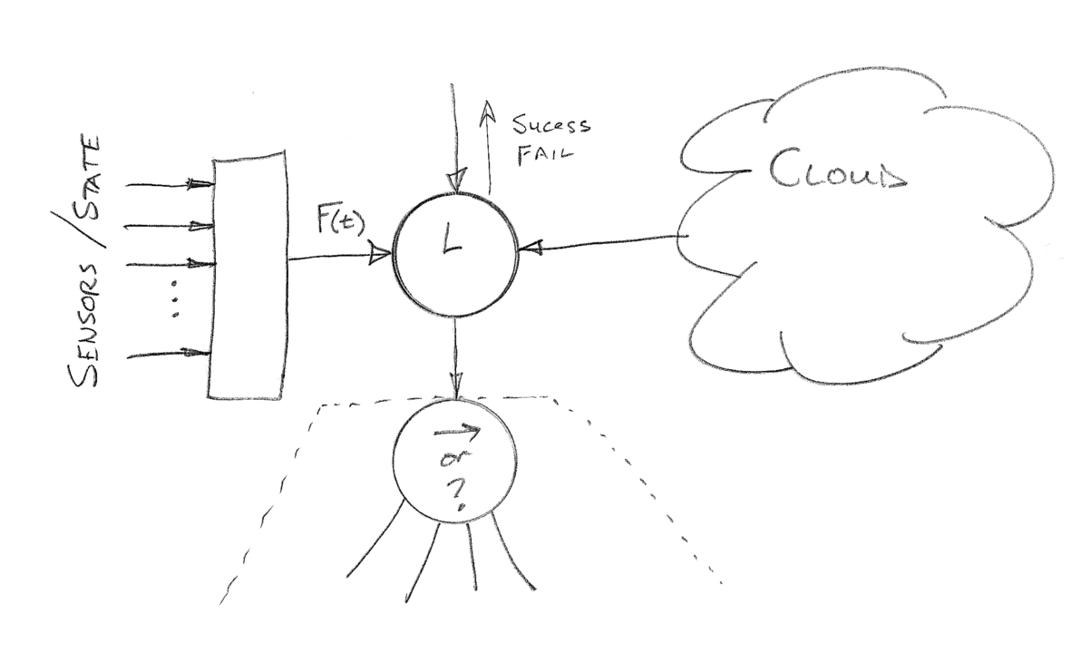
Figure 1: Learning Node which can be attached to any BT node.

As an alternative to adding learning functions to existing node types, we can create a new node, the ‘L’ (Learning) Node (Figure 1). The L node works as follows. Using the history of its single child node (which in general is any sub-tree of the BT), the L node accumulates Success and Failure outcomes from the child and accumulates an estimate of the probability

$$P(S|F)$$ (4)

$P(S|F)$ can be estimated in a number of was including Parametric (Gaussian or mixture of Gaussians over the feature space), or particle filters. The L node can also obtain data for the estimate from a cloud connected population of similar robots having the same child node in their behavior trees and situated in similar environments.

3 Simulations

3.1 New Node Features

A basic simulator was developed using the behavior3 python BT library[7] (github.org). Several new features were added to the node base class:

• Node keeps track of how many times it has been ticked

• Node keeps track of how many times it has reported success.

• Node has a method to compute $P(S)=N_{success}/N_{ticks}$. If $N_{ticks}==0$, $P(S)=0.5$.

• Node keeps an array $N_{t2}$ which stores the number of ticks in the presence of each value of the sensing feature vector $F$.

• Node keeps an array $N_{s2}$ which stores the number of successes in the presence of each value of the sensing feature vector $F$.

• Node has a method to return an array of estimated probabilities:

  $$P_{ij}=\frac{N_{s2}[j]}{N_{t2}[j]}=\hat{P}(S_{i}|F_{j})$$ (5)

  If $N_{t2}[j]==0$, $P(S_{i}|F_{j})=0.5$.

• Every node has an associated “Cost,” $C$, for each tick. Cost for a node can be zero. Cost for each leaf node is determined either by the system designer, or could be calculated, for example by an energy meter built into the robot. A higher level node can sum up the cost of each of its children. Although we will not address it in this paper, the Cost estimate can also be conditioned on the sensor cluster, $F$.

• Node has a notion of “Utility” at each tick, $t$. Utility could be computed in one of two modes: “Ratio” mode in which Utility is

  $$U=\frac{P(S)}{C}\qquad\mathrm{or}\qquad\frac{P(S|F)}{C}$$ (6)

  and “Negative Cost” mode: in which Utility is

  $$U=-P(S)C\qquad\mathrm{or}\qquad-P(S|F)C$$ (7)

3.2 Adaptive Selector Types

Using the new node features, we developed several new types of Selector nodes:

• S1. reorder the leaves according to $P(S)$.

• S2. reorder the leaves according to $P(S_{i}|F_{j})$

• S2g. same as S2, but with Greedy behavior.

• S3. reorder the leaves according to $C_{i}$

• S4. reorder the leaves according to $U_{i}$

• S5. same as S4, but compute utility using $P(S_{i}|F_{i})$

In addition, we define node type S0 as the regular “dumb” Selector node.

3.3 Results

Figure 2: BT for robot walking over simulated terrain. Three different stepping behaviors (1,2,3) have different effectiveness for different terrains. They are coordinated by a Selector node (labeled ?).

A basic, probabilistic simulator was constructed for the task of a humanoid robot walking across several terrains: e.g. Snow, Grass, and Parking Lot. The BT (Figure 2) selects between three “stepping” behaviors (W1 — W3) and a “Physics Matrix” gives the probability of a successful step by each stepping behavior on each terrain. It is assumed that the robot can recover from a failed step but makes no forward progress in doing so.

The test consisted of 250 simulated traversals of a test track consisting of 250 steps. The test track consists of stretches of various lengths of each terrain. The initial Physics Matrix was:

$$Ph(n,F)=\begin{bmatrix}0.8&0.1&0.1\\ 0.1&0.8&0.1\\ 0.1&0.1&0.8\\ \end{bmatrix}$$ (8)

The Physics Matrix $Ph(n,F)$ indicates for example that node W1 has a 0.8 probability of a successful step on terrain 1. Note that although $Ph(n,F)\leq 1$ is a requirement, there is no constraint on the rows or column sums of $Ph$. For S4 and S5, the cost of each walking method (leaf) was set up as follows: $C$(W1) = 4, $C$(W2) = 2, $C$(W3) = 1.

The measures of success were the inverse number of ticks required to traverse the test track, and the total average cost per tick. The derived metric of overall average Utility was also computed. The number of ticks was totaled and the ticks required at each step was averaged over the 250 trials. The course was unchanged over the 250 trials.

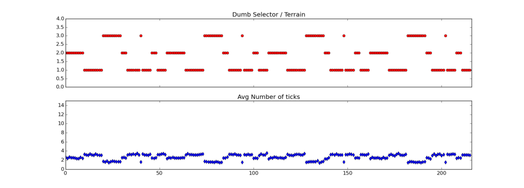
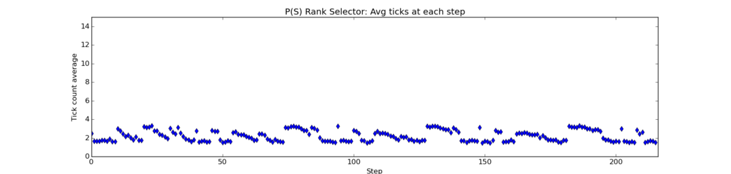
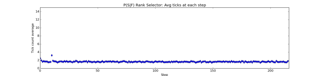
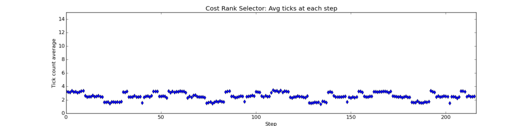
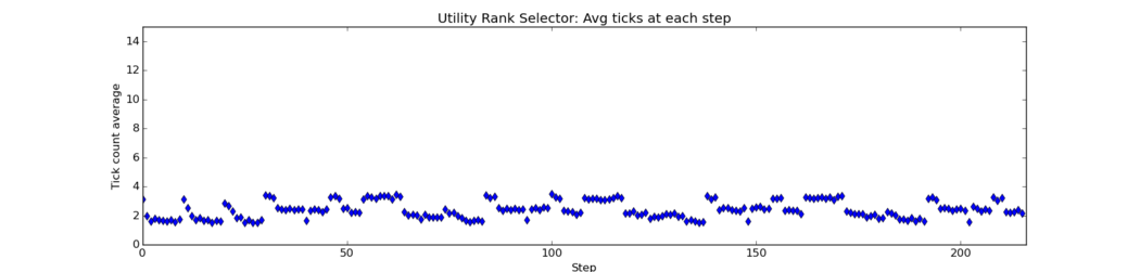
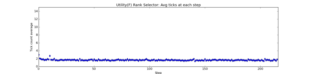
Figure 3: Simulation runs on the walking humanoid robot task for each of the five Selector types. Terrain sequence (red) illustrates the fixed sequence of three terrain types. For each simulation result, (blue), X axis is traversal distance in steps. Y axis is average number of ticks required to complete each step. Terrain sequence is illustrated in uppermost plot.

	avg ticks	avg cost	avg Util/tick x 1000
S0: dumb Selector	577	1286	18.25
S1: P(S) order	478	1151	18.51
S2: P(S$|$F) order	358	663	36.73
S3: Cost order	549	1031	22.62
S4: Utility order	522	1026	22.47
S5: Utility(F) order	361	844	36.57
S2g00: P(S$|$F) Greedy	490	911	59.17
S2g25: P(S$|$F) Greedy	284	675	49.60

Table 1: Simulated walking performance averaged over the 250 trials for each smart Selector (utility values are multiplied by 1000).

The results of simulations in which each Selector type traversed the course 250 times are given in Figure 3 and Table 1.

S0: “Dumb” Selector

The average number of ticks remains the same for each terrain level and does not adapt over time as expected from its fixed leaf execution sequence. With the dumb Selector, the robot took an average of 577 ticks to traverse the course length of 216 steps, accumulated an average cost of 1286, and an average utility of 0.01825 on each tick. These values serve as a baseline for comparison with the smart Selectors (below).

S1: P(S) Selector

The first smart Selector reorders its leaves in descending order of their overall probability of success. It can be seen that the number of clicks adapts over the time that terrain remains constant but then increases at each terrain change.

The average number of ticks per course traversal was substantially reduced to 478. Cost and Utility were approximately the same.

S2: P(S$|$F) Selector

This Selector tries its leaves in descending order of their probability of success conditioned on a simulated sensor measurement of the terrain type (which is 100% accurate). The average tick count quickly adapts to a steady state value of a little less than two clicks per step. Note transients of worse performance are observed at the first transitions between terrain types.

Average ticks per traversal for S2 were the lowest of all at 358. Cost and utility were also the best.

S3: Cost Selector

This Selector executes its leaves in increasing order of leaf cost. This should not appreciably affect click rate compared to the dumb Selector, but different average click rates are associated with each terrain type because the cost ranking is different than the initial order.

The Cost-based Selector had significantly lower cost (1031) than the dumb Selector, but the performance of the cost Selector depends on the relative cost assigned to the nodes which was arbitrary in this experiment.

S4: Utility Selector

Both Utility Selectors (S4 and S5) were initially studied with Ratio mode (6). The Utility Selector combines the fixed cost weights with the experience-based probability estimates. As with S1, the tick count per step adapts downwards during the time terrain remains constant.

Because of the symmetry of the chosen physics matrix, and the roughly equal distribution of terrain states in the trajectory, $P(S)$ is about the same for each leaf and thus the numerical results for utility order are very similar to those of cost order.

S5: Utility(F) Selector

This Selector derives utility based on the sensor-conditioned success probability. Similarly to the S2 Selector, it rapidly converges to a steady state value.

Although S5 has a very low average tick count (361), its overall performance is not significantly better than S2, even for average Utility.

S2g: Greedy P(S$|$F) Selector)

This Selector repeatedly ticks only the highest probability leaf. The performance of this Selector is not good (Figure 4, top). Because it is constantly selecting only the highest probability, it is not exercising the other leaves enough for them to have robust probability estimates. Another set of 250 runs was performed in which the Greedy mode was not enabled until 25 steps were completed with the normal S2 Selector. This mode allowed the probability estimates to converge. Subsequently the greedy mode performed extremely well.

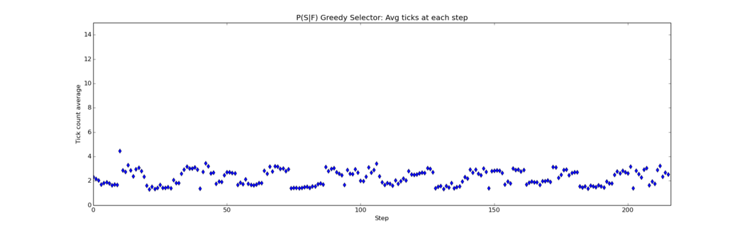
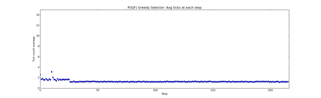
Figure 4: Simulated walking runs with the Greedy P(S—F) Selector. Performance is poor (top) because all the leaves are not exercised enough to generate robust estimates of $P(S|F)$. When Greedy mode is enabled after 25 initial steps with the normal S2 Selector (bottom trace) performance is excellent.

3.3.1 Ratio vs Linear Utilities

All Selectors were re-run with the Utility computation changed to Negative Cost mode (7). The average tick counts and average cost values were essentially unchanged (max difference 5 ticks/ 9 cost points). The utility values were not directly comparable, but the ranking of highest to lowest utility changed dramatically, in Ratio Mode, the highest two Selectors for Utility were S2g and S4 (Greedy P(S—F) and Utility(F) order). In Negative Cost Mode, the highest two Selectors were S3 and S4 (Cost order and Utility order) and number 3 was S5 (Utility(F) order). The relative utility achieved by the Selectors is thus highly sensitive to the Utility definition.

3.3.2 Cost Weights

We investigated the sensitivity of these results to choice of costs on the three nodes which were initially [2,4,1] for the three nodes respectively. We re-ran the tests above with the costs reset to [2,1,4]. The average tick counts were mostly unchanged. The largest difference was 5 ticks (out of 515) except for S3, Cost order, which decreased by 32 ticks on average when the costs were changed.

Average cost per run was less consistent. The average cost increased for S0 (dumb Selector) and for S2g00 (Greedy Selector without training interval), but decreased substantially for the others. Average Utility decreased for the same two Selectors, but increased for the others. The relative performance of the various Selectors remained approximately the same except for a drop in ranking of the S2g00 (untrained Greedy) Selector.

3.3.3 Symmetry of Physics Matrix

In the previous tests, the Physics matrix was given by (8). Using the first set of cost weights: [2,4,1] , we changed the physics matrix to

$$Ph(n,F)=\begin{bmatrix}0.6&0.1&0.1\\ 0.4&0.7&0.4\\ 0.1&0.1&0.8\\ \end{bmatrix}$$ (9)

to introduce better and weaker nodes. Node two is now reasonably good at all terrains although not the best on terrains 1 and 3.

When this change was introduced to the system, average tick counts per run went up for all Selectors except the dumb Selector. Cost also increased for all Selectors. Average utility declined modestly for all Selectors.

3.3.4 More Complex Scenario

A more complex scenario derived from the fire rescue scenario studied in Pereira and Engel[7] was simulated. In our modified version of this scenario (Figure 5), the robot walks to a fire (in the same was as the walking scenario above). The distance to the fire is 100 steps. If the robot fails to reach the fire in walk_limit steps, the robot flies to the fire using its jet-pack (at much higher cost). The cost of a step is set to one and the cost of flying to the destination is 350. Flying succeeds with probability 0.9. A value of the walk limit at which the robot must convert to flight about 50% of the time with the dumb Selector was experimentally determined to be 120 steps. Simulations were also run with higher walk_limits to reduce the number of flight conversions.

At the fire, there are three fire types. The robot uses one of three extinguishers with a fire fighting physics matrix of

$$Pf(n,F)=\begin{bmatrix}1.00&0.05&0.05\\ 0.05&1.00&0.05\\ 0.05&0.05&1.00\\ \end{bmatrix}$$ (10)

The interpretation of the fire physics matrix is that extinguisher A has a 100% probability of extinguishing fire type A, and a small probability of extinguishing fire types B and C, etc. The intent of setting at least one element in each column to 1.0 is so that success of the tree as a whole depends only on the transport node.

Figure 5: Behavior tree for fire rescue task (adapted from [7]).

	limit	avg ticks	avg cost	avg Util	walk ticks	fly ticks	fails
Sel00: Dumb Selector	150	228	245	0.41	1000	0	0
Sel00: Dumb Selector	120	224	441	0.28	1000	574	52
Sel01: P(S) ranking	120	22	388	0.26	89	1000	45
Sel02: P(S$|$F) ranking	120	18	376	0.27	103	1000	63
Sel02: P(S$|$F) ranking	150	18	376	0.27	97	1000	0
Sel02: P(S$|$F) ranking	900	167	176	0.57	1000	1	0
Sel03: Cost ranking	120	165	379	0.35	1000	568	71
Sel04: Utility ranking	120	28	393	0.26	117	999	60
Sel05: Utility(F) ranking	120	16	373	0.27	89	999	38

Table 2: Simulated fire fighting scenario. “limit” is the number of ticks allowed to reach fire before robot switches to flight. 1000 trials per Selector.

Results

The firefighting task of Figure 5 was simulated 1000 times for each BT and the walk_limit was changed to understand the frequency of conversion to flying.

S0

S0 had no conversions to flight when walk_limit was 150, but about 57% flight conversions with walk_limit at 120. The average cost increased by 196 ticks as the number of expensive flights increased (flight cost = 350). Failures increased to about 10% of flights since the flight mode had only 90% success probability. All walking trials were overall successful since extinguish node is guaranteed to succeed.

S1

S1 (P(S) ranking) was evaluated with walk_limit of 120 in which the probability of successfully walking to the fire is about 50%. In this case the $P(S)$ Selector adapted to the higher success rate of flying and flew on all 1000 trials. Average cost was still lower than the equivalent dumb Selector trials, presumably because of fewer wasted steps prior to flying.

S2

S2 strongly preferred flight unless the walk_limit was set to the very high value of 900.

S3

S3 performed similar to the Dumb Selector although with slightly lower cost.

S4 and S5

Utility ranking was evaluated in Ratio mode. Both Utility ranking modes performed similarly to the S2 ($P(S|F)$) ranking.

3.4 Simulation: Conclusions

3.4.1 Terrain Navigation

Smart Selectors performed robust adaptation to the simulated walking task under a variety of circumstances. From the point of view of how many ticks were required to navigate the terrain, the worst Selector under all circumstances was the dumb Selector (and its close relative the untrained Greedy Selector). The two best Selectors were the S2g25 (trained greedy) Selector, and the S2 $P(S|F)$ Selectors under all conditions tested. In Ratio Mode, the two Selectors designed to minimize cost or maximize utility did not do so relative to the two best performing nodes. When measured by average tick count per traversal, the performance of the Cost Selector was most sensitive to change in the node costs as expected.

However, when the Utility measure was changed to Negative Cost Mode (7), S3-S5, the Selectors which chose Cost and Utility had the highest average Utility, and the Dumb Selector and the untrained greedy Selector the worst. This suggests a linear Utility measure operates more intuitively.

3.4.2 Firefighting

The more complex fire-fighting scenario was simulated in order to study the extension of the Selectors tested in the terrain scenario to a slightly more complex task. It is less straightforward to predict the effects of smart Selectors as the scenario gets more complex, but increasing the walk_limit simulation parameter, which increases the chance of successfully walking to the fire, produced the expected changes in tick counts, and total costs.

4 Discussion

This paper has explored adaptation in Behavior Tree Selector nodes through some simulation experiments. The simulations showed that adaptive selectors could considerably improve the performance of Selector nodes through a variety of methods. Evaluating node probabilities conditioned on quantized sensor information was effective. Measures of cost and utility were less effectively optimized by experience through behavior trees.

A greedy selector, which selects only its node of highest probability, was potentially very effective, but only when activated after a period of learning in which all leaves were activated enough times to develop robust probability estimates.

We plan to further explore these results with physical experimental platforms, and to explore their applicability to medical robotics.

Acknowledgements

We are pleased to acknowledge support for this work from the Korean Institute of Science and Technology (KIST, Dr. Hujoon project), the U.S National Institutes of Health NIBIB R01 EB016457 NRI-Small, and the National Science Foundation (grant number 1227406) under a subcontract from Stanford University.

References

- [1] Damián Isla. Building a better battle: The halo 3 ai objectives system. http://web.cs.wpi.edu/~rich/courses/imgd4000-d09/lectures/halo3.pdf.
- [2] Chong-U Lim, Robin Baumgarten, and Simon Colton. Evolving behaviour trees for the commercial game defcon. In European Conference on the Applications of Evolutionary Computation, pages 100–110. Springer, 2010.
- [3] Alejandro Marzinotto, Michele Colledanchise, Christian Smith, and Petter Ögren. Towards a unified behavior trees framework for robot control. In 2014 IEEE International Conference on Robotics and Automation (ICRA), pages 5420–5427. IEEE, 2014.
- [4] Michele Colledanchise, Alejandro Marzinotto, and Petter Ögren. Performance analysis of stochastic behavior trees. In 2014 IEEE International Conference on Robotics and Automation (ICRA), pages 3265–3272. IEEE, 2014.
- [5] J Andrew Bagnell, Felipe Cavalcanti, Lei Cui, Thomas Galluzzo, Martial Hebert, Moslem Kazemi, Matthew Klingensmith, Jacqueline Libby, Tian Yu Liu, Nancy Pollard, et al. An integrated system for autonomous robotics manipulation. In 2012 IEEE/RSJ International Conference on Intelligent Robots and Systems, pages 2955–2962. IEEE, 2012.
- [6] Danying Hu, Yuanzheng Gong, Blake Hannaford, and Eric J Seibel. Semi-autonomous simulated brain tumor ablation with ravenii surgical robot using behavior tree. In 2015 IEEE International Conference on Robotics and Automation (ICRA), pages 3868–3875. IEEE, 2015.
- [7] Renato de Pontes Pereira and Paulo Martins Engel. A framework for constrained and adaptive behavior-based agents. arXiv Preprint: 1506.02312 [cs.AI], 2015.
- [8] Michele Colledanchise, Ramviyas Parasuraman, and Petter Ögren. Learning of behavior trees for autonomous agents. arXiv Preprint: 1504.05811 [cs.RO], 2015.