Disease Trajectory Maps

Abstract

Medical researchers are coming to appreciate that many diseases are in fact complex, heterogeneous syndromes composed of subpopulations that express different variants of a related complication. Time series data extracted from individual electronic health records (EHR) offer an exciting new way to study subtle differences in the way these diseases progress over time. In this paper, we focus on answering two questions that can be asked using these databases of time series. First, we want to understand whether there are individuals with similar disease trajectories and whether there are a small number of degrees of freedom that account for differences in trajectories across the population. Second, we want to understand how important clinical outcomes are associated with disease trajectories. To answer these questions, we propose the Disease Trajectory Map (DTM), a novel probabilistic model that learns low-dimensional representations of sparse and irregularly sampled time series. We propose a stochastic variational inference algorithm for learning the DTM that allows the model to scale to large modern medical datasets. To demonstrate the DTM, we analyze data collected on patients with the complex autoimmune disease, scleroderma. We find that DTM learns meaningful representations of disease trajectories that the representations are significantly associated with important clinical outcomes.

1 Introduction

Time series data is becoming increasingly important in medical research and practice. This is due, in part, to the growing adoption of electronic health records (EHRs), which capture snapshots of an individual’s state over time. These snapshots include clinical observations (apparent symptoms and vital sign measurements), laboratory test results, and treatment information. In parallel, medical researchers are beginning to recognize and appreciate that many diseases are in fact complex, highly heterogeneous syndromes (Craig, 2008) and that individuals may belong to disease subpopulations or subtypes that express similar sets of symptoms over time (see e.g. Saria and Goldenberg (2015)). Examples of such diseases include asthma (Lötvall et al., 2011), autism (Wiggins et al., 2012), and COPD (Castaldi et al., 2014). The data captured in EHRs can help better understand these complex diseases. EHRs contain a multitude of types of observations and the ability to track their progression can help bring in to focus the subtle differences across individual disease expression.

In this paper, we focus on two exploratory questions that we can begin to answer using repositories of biomedical time series data. First, we want to discover whether there are individuals with similar disease trajectories and whether there are a small number of degrees of freedom that account for differences across a heterogeneous population. A better understanding of the types of trajectories and how they differ can yield insights into the biological underpinnings of the disease. In turn, this may motivate new targeted therapies. In the clinic, physicians can analyze an individual’s clinical history to better understand the “flavor” of the disease being expressed and can use this knowledge to make more accurate prognoses and guide treatment decisions. Second, we would like to know whether individuals with similar clinical outcomes (e.g. death, severe organ damage, or development of comorbidities) have similar disease trajectories. In complex diseases, individuals are often at risk of developing a number of severe complications and clinicians rarely have access to accurate prognostic biomarkers. Discovering associations between target outcomes and trajectory patterns may both generate new hypotheses regarding the causes of these outcomes and help clinicians to better anticipate the event using an individual’s clinical history.

Contributions.

Our approach to simultaneously answering these questions is to embed individual disease trajectories into a low-dimensional vector space wherein similarity in the embedded space implies that two individuals have similar trajectories. Such an embedding would naturally answer our first question, and the results could also be used to answer the second by comparing distributions over embeddings across groups defined by different outcomes. To produce such an embedding, we introduce a novel probabilistic model of biomedical time series data, which we term the Disease Trajectory Map (DTM). In particular, the DTM models the trajectory of a single clinical marker, which is an observation or measurement recorded over time by clinicians that are used to track the progression of a disease (see e.g. Schulam et al. (2015)). Examples of clinical markers are pulmonary function tests or creatinine laboratory test results, which track lung and kidney function respectively. The DTM discovers low-dimensional (2D or 3D) latent representations of clinical marker trajectories that are easy to visualize. Moreover, the model learns an expressive family of distributions over trajectories that is parameterized by the low-dimensional representation. This allows the DTM to capture a wide variety of trajectory shapes, making it suitable for studying complex diseases where expression varies widely across the population. We describe a stochastic variational inference algorithm for estimating the posterior distribution over the parameters and individual-specific representations, which allows our model to be easily applied to large biomedical datasets. To demonstrate the DTM, we analyze clinical marker data collected on individuals with the complex autoimmune disease scleroderma (see e.g. Allanore et al. (2015)). We find that the learned representations capture interesting subpopulations consistent with previous findings, and that the representations suggest associations with important clinical outcomes.

1.1 Background and Related Work

Clinical marker data extracted from EHRs is a by-product of an individual’s interactions with the healthcare system. As a result, the time series are often irregularly sampled (the time between samples varies within and across individuals), and may be extremely sparse (it is not unusual to have a single observation for an individual). To aid the following discussion, we briefly introduce notation for this type of data. We use $m$ to denote the number of individual disease trajectories recorded in a given dataset. For each individual, we use $n_{i}$ to denote the number of observations. We collect the observation times for subject $i$ into a column vector $\bm{\mathrm{t}}_{i}$ (sorted in non-decreasing order) and the corresponding measurements into a column vector $\bm{\mathrm{y}}_{i}$: $\bm{\mathrm{t}}_{i}\triangleq[t_{i1},\ldots,t_{in_{i}}]^{\top}$ and $\bm{\mathrm{y}}_{i}\triangleq[y_{i1},\ldots,y_{in_{i}}]^{\top}$. Our goal is to embed the pair $(\bm{\mathrm{t}}_{i},\bm{\mathrm{y}}_{i})$ into a low-dimensional vector space wherein similarity between two embeddings $(\bm{\mathrm{x}}_{i},\bm{\mathrm{x}}_{j})$ implies that the trajectories have similar shapes. This is commonly done using basis representations of the trajectories.

Fixed basis representations.

In the statistics literature, trajectory data is often referred to as unbalanced longitudinal data, and it is commonly analyzed in that community using linear mixed models (LMMs) (Verbeke and Molenberghs, 2009). In their simplest form, LMMs assume the following probabilistic model:

$$\bm{\mathrm{w}}_{i}\mid\mathrm{\Sigma} \sim\mathcal{N}(\mathrm{0},\mathrm{\Sigma})\,\,\,,\,\,\,\bm{\mathrm{y}}_{i}\mid\mathrm{B}_{i},\bm{\mathrm{w}}_{i},\mu,\sigma^{2}\sim\mathcal{N}(\mu+\mathrm{B}_{i}\bm{\mathrm{w}}_{i},\sigma^{2}\mathrm{I}_{n_{i}}).$$ (1)

The matrix $\mathrm{B}_{i}\in\mathbb{R}^{n_{i}\times d}$ is known as the design matrix, and can be used to capture non-linear relationships between the observation times $\bm{\mathrm{t}}_{i}$ and measurements $\bm{\mathrm{y}}_{i}$. Its rows are comprised of $d$-dimensional basis expansions of each observation time $\mathrm{B}_{i}=[\bm{\mathrm{b}}(t_{i1}),\cdots,\bm{\mathrm{b}}(t_{in_{i}})]^{\top}$. Common choices of $\bm{\mathrm{b}}(\cdot)$ include polynomials, splines, wavelets, and Fourier series. The particular basis used is often carefully crafted by the analyst depending on the nature of the trajectories and on the desired structure (e.g. invariance to translations and scaling) in the representation (Brillinger, 2001). The design matrix can therefore make the LMM remarkably flexible despite its simple parametric probabilistic assumptions. Moreover, the prior over $\bm{\mathrm{w}}_{i}$ and the conjugate likelihood make it straightforward to fit $\mu$, $\mathrm{\Sigma}$, and $\sigma^{2}$ using EM or Bayesian posterior inference.

After estimating the model parameters, we can estimate the coefficients $\bm{\mathrm{w}}_{i}$ of a given clinical marker trajectory using the posterior distribution, which embeds the trajectory in a Euclidean space. To flexibly capture complex trajectory shapes, however, the basis must be high-dimensional, which makes interpretability of the embeddings challenging. We can use low-dimensional summaries such as the projection on to a principal subspace, but these are not necessarily substantively meaningful. Indeed, much research has gone into developing principal direction post-processing techniques (e.g. Kaiser (1958)) or alternative estimators that enhance interpretability (e.g. Carvalho et al. (2012)).

Data-adaptive basis representations.

A set of related, but more flexible, techniques comes from functional data analysis where observations are functions (i.e. trajectories) assumed to be sampled from a stochastic process and the goal is to find a parsimonious representation for the data (Ramsay et al., 2002). Functional principal component analysis (FPCA), one of the most standard techniques in functional data analysis, expresses functional data in the orthonormal basis given by the eigenfunctions of the auto-covariance operator. This representation is optimal in the sense that no other representation captures more variation (Ramsay, 2006). The idea itself can be traced back to early independent work by Karhunen and Loeve and is also referred to as the Karhunen-Loeve expansion (Watanabe, 1965). While numerous variants of FPCA have been proposed, the one that is most relevant to the problem at hand is that of sparse FPCA (Castro et al., 1986; Rice and Wu, 2001) where we allow sparse irregularly sampled data as in longitudinal data analysis. To deal with the sparsity, Rice and Wu (2001) proposed the mixed effect model which leverages statistical strength from all observations for function estimation. The mixed effect model often suffers from numerical instability of covariance matrices in high dimensions; James et al. (2000) addressed this by constraining the rank of the covariance matrices—this is often referred to as the reduced rank model. The reduced rank model was further extended by Zhou et al. (2008) to a two-dimensional sparse principal component model. Although the reduced rank model embeds trajectories using a data-driven basis, the basis is restricted to lie in a linear subspace of a fixed basis, which may be overly restrictive. Other approaches to learning a functional basis include Bayesian estimation of B-spline parameters (e.g. (Bigelow and Dunson, 2012)) and placing priors over reproducing kernel Hilbert spaces (e.g. (MacLehose and Dunson, 2009)). Although flexible, these two approaches do not learn a compact representation.

Cluster-based representations.

Mixture models and clustering approaches are also commonly used to represent and discover structure in time series data. Marlin et al. (2012) cluster time series data from the ICU using a mixture model and use cluster membership to predict outcomes. Schulam and Saria (2015) describe a probabilistic model that represents trajectories using a hierarchy of features, which includes “subtype” or cluster membership. LMMs have also been extended to have nonparametric Dirichlet process priors over the coefficients (e.g. Kleinman and Ibrahim (1998)), which implicitly induce clusters in the data. Although these approaches flexibly model trajectory data, the structure they recover is a partition, which does not allow us to compare all trajectories in a coherent way as we can in a vector space.

Lexicon-based representations.

Another line of research has investigated the discovery of motifs or repeated patterns in continuous time-series data for the purposes of succinctly representing the data as a string of elements of the discovered lexicon. These include efforts in the speech processing community to identify sub-word units (parts of the words at the same level as phonemes) in a data-driven manner (Varadarajan et al., 2008; Levin et al., 2013). In computational healthcare, Saria et al. (2011) propose a method for discovering deformable motifs that are repeated in continuous time-series data. These methods are, in spirit, similar to discretization approaches such as symbolic aggregate approximation (SAX) (Lin et al., 2007) and piecewise aggregate approximation (PAX) (Keogh et al., 2001) that are popular in data mining, and aim to find compact description of sequential data, primarily for the purposes of indexing, search, anomaly detection, and information retrieval. The focus in this paper is to learn representations for entire trajectories rather than discover a lexicon. Furthermore, we are interested in learning a representation for individuals and capturing latent similarities between two patients in terms of Euclidean distances in the learnt representation.

2 Disease Trajectory Maps

To motivate Disease Trajectory Maps, we begin from the reduced-rank formulation of linear mixed models as proposed by James et al. (2000). In particular, let $\mu\in\mathbb{R}$ be the marginal mean of the observations, $\mathrm{F}\in\mathbb{R}^{d\times q}$ be a rank-$q$ matrix, and $\sigma^{2}$ be the variance of measurement errors. As a reminder, $\bm{\mathrm{y}}_{i}\in\mathbb{R}^{n_{i}}$ denotes the vector of observed trajectory measurements, $\mathrm{B}_{i}\in\mathbb{R}^{n_{i}\times d}$ denotes the subject’s design matrix, and $\bm{\mathrm{x}}_{i}\in\mathbb{R}^{q}$ denotes the representation or embedding of the subject. We begin with the reduced-rank conditional model: $\bm{\mathrm{y}}_{i}\mid\mathrm{B}_{i},\bm{\mathrm{x}}_{i},\mu,\mathrm{F},\sigma^{2}\sim\mathcal{N}(\mu+\mathrm{B}_{i}\mathrm{F}\bm{\mathrm{x}}_{i},\sigma^{2}\mathrm{I}_{n_{i}}).$ In the reduced-rank model, we assume an isotropic normal prior over $\bm{\mathrm{x}}_{i}$ and marginalize to obtain the observed-data log-likelihood, which is then optimized with respect to $\mathrm{F}$. Here, just as was done by Lawrence (2004) to derive the GPLVM, we swap the marginalization for optimization and vice versa. By assuming a normal prior $\mathcal{N}(\bm{\mathrm{0}},\alpha\mathrm{I}_{k})$ over the rows of $\mathrm{F}$ and marginalizing we obtain:

$$\bm{\mathrm{y}}_{i}\mid\mathrm{B}_{i},\bm{\mathrm{x}}_{i},\mu,\sigma^{2},\alpha\sim\mathcal{N}(\mu,\alpha\langle\bm{\mathrm{x}}_{i},\bm{\mathrm{x}}_{i}\rangle\mathrm{B}_{i}\mathrm{B}^{\top}_{i}+\sigma^{2}\mathrm{I}_{n_{i}}).$$ (2)

Note that by marginalizing over $\mathrm{F}$, we induce a joint distribution over all trajectories in the dataset. Moreover, this joint distribution is a Gaussian process with mean $\mu$ and the following covariance function defined across trajectories:

$$\operatorname{Cov}(\bm{\mathrm{y}}_{i},\bm{\mathrm{y}}_{j}\mid\mathrm{B}_{i},\mathrm{B}_{j},\bm{\mathrm{x}}_{i},\bm{\mathrm{x}}_{j},\mu,\sigma^{2},\alpha)=\alpha\langle\bm{\mathrm{x}}_{i},\bm{\mathrm{x}}_{j}\rangle\mathrm{B}_{i}\mathrm{B}^{\top}_{j}+\mathbb{I}[i=j]\,(\sigma^{2}\mathrm{I}_{n_{i}}).$$ (3)

This reformulation of the reduced-rank LMM suggests a natural alternative to learning the representations $\bm{\mathrm{x}}_{i}$ of the subjects. Just as in the GPLVM, we can maximize the log-probability of all trajectories with respect to the hyperparameters $\{\mu,\sigma^{2},\alpha\}$ and the representations $\{\bm{\mathrm{x}}_{i}:i\in[m]\}$. More importantly, however, the reformulation allows us to relate the representation to the basis coefficients non-linearly by using the “kernel trick” to reparameterize the covariance function. Let $k(\cdot,\cdot)$ denote a non-linear kernel defined over the representations with parameters $\bm{\mathrm{\theta}}$, then we have:

$$\operatorname{Cov}(\bm{\mathrm{y}}_{i},\bm{\mathrm{y}}_{j}\mid\mathrm{B}_{i},\mathrm{B}_{j},\bm{\mathrm{x}}_{i},\bm{\mathrm{x}}_{j},\mu,\sigma^{2},\bm{\mathrm{\theta}})=k(\bm{\mathrm{x}}_{i},\bm{\mathrm{x}}_{j})\mathrm{B}_{i}\mathrm{B}^{\top}_{j}+\mathbb{I}[i=j]\,(\sigma^{2}\mathrm{I}_{n_{i}}).$$ (4)

Let $\bm{\mathrm{y}}\triangleq[\bm{\mathrm{y}}_{1}^{\top},\ldots,\bm{\mathrm{y}}_{m}^{\top}]^{\top}$ denote the column vector obtained by concatenating the measurement vectors from each trajectory. The joint distribution over $\bm{\mathrm{y}}$ is a multivariate normal:

$$\bm{\mathrm{y}}\mid\mathrm{B}_{1:m},\bm{\mathrm{x}}_{1:m},\mu,\sigma^{2},\bm{\mathrm{\theta}}\sim\mathcal{N}(\mu,\mathrm{\Sigma}_{\text{DTM}}+\sigma^{2}\mathrm{I}_{n}),$$ (5)

where $\mathrm{\Sigma}_{\text{DTM}}$ is a full-rank covariance matrix that depends on the design matrices $\mathrm{B}_{1:m}$, the representations $\bm{\mathrm{x}}_{1:m}$, and the kernel $k(\cdot,\cdot)$. In particular, $\mathrm{\Sigma}_{\text{DTM}}$ is a block-structured matrix with $m$ row blocks and $m$ column blocks. The block at the $i^{\text{th}}$ row and $j^{\text{th}}$ column is the covariance between $\bm{\mathrm{y}}_{i}$ and $\bm{\mathrm{y}}_{j}$ defined above. We complete the model by placing isotropic Gaussian priors over $\bm{\mathrm{x}}_{i}$. Note that this model is similar to the Bayesian GPLVM (Titsias and Lawrence, 2010), but models functional data instead of finite-dimensional vectors.

2.1 Learning and Inference in the DTM

As formulated, the model will scale poorly to large datasets. Inference within each iteration of an optimization algorithm, for example, requires storing and inverting $\mathrm{\Sigma}_{\text{DTM}}$, which requires $O(n^{2})$ space and $O(n^{3})$ time respectively, where $n\triangleq\sum_{i=1}^{m}n_{i}$ is the number of clinical marker observations. For modern datasets, where $n$ can be in the hundreds of thousands or millions, this is unacceptable. In this section, we approximate the log-likelihood using techniques from Hensman et al. (2013) that allows us to apply stochastic variational inference (SVI) (Hoffman et al., 2013).

Recent work in scaling Gaussian processes to large datasets focuses on the idea of inducing points (Snelson and Ghahramani, 2005; Titsias, 2009), which are a relatively small number of artificial observations of the Gaussian process that act as a bottleneck and approximately capture the information contained in the training data. Let $\bm{\mathrm{f}}\in\mathbb{R}^{m}$ denote observations of the GP at inputs $\{\bm{\mathrm{x}}_{i}\}_{i=1}^{m}$ and $\bm{\mathrm{u}}\in\mathbb{R}^{p}$ denote inducing points at inputs $\{\bm{\mathrm{z}}_{i}\}_{i=1}^{p}$. Titsias (2009) constructs the inducing points as variational parameters by introducing an augmented probability model:

$$\bm{\mathrm{u}}\sim\mathcal{N}(\bm{\mathrm{0}},\mathrm{K}_{pp})\,\,\,,\,\,\,\bm{\mathrm{f}}\mid\bm{\mathrm{u}}\sim\mathcal{N}(\mathrm{K}_{mp}\mathrm{K}^{{-1}}_{pp}\bm{\mathrm{u}},\tilde{\mathrm{K}}_{mm}),$$ (6)

where $\mathrm{K}_{pp}$ is the Gram matrix between inducing points, $\mathrm{K}_{mm}$ is the Gram matrix between observations, $\mathrm{K}_{mp}$ is the cross Gram matrix between observations and inducing points, and $\tilde{\mathrm{K}}_{mm}\triangleq\mathrm{K}_{mm}-\mathrm{K}_{mp}\mathrm{K}^{{-1}}_{pp}\mathrm{K}_{pm}$. Titsias (2009) then marginalizes over $\bm{\mathrm{u}}$ to construct a low-rank approximate covariance matrix, which is computationally cheaper to invert using the Woodbury identity. Hensman et al. (2013) extends these ideas by maintaining a variational distribution over $\bm{\mathrm{u}}$ that d-separates the observations and satisfies the conditions required to apply SVI (Hoffman et al., 2013). Let $\bm{\mathrm{y}}_{f}=\bm{\mathrm{f}}+\bm{\mathrm{\epsilon}}$ where $\bm{\mathrm{\epsilon}}$ is iid Gaussian noise with variance $\sigma^{2}$, then the key result from Hensman et al. (2013) that we use here is the following bound:

$$\textstyle\log p(\bm{\mathrm{y}}_{f}\mid\bm{\mathrm{u}})\geq\sum_{i=1}^{m}\mathbb{E}_{p(f_{i}\mid\bm{\mathrm{u}})}[\log p(y_{fi}\mid f_{i})].$$ (7)

In the interest of space, we refer the interested reader to Hensman et al. (2013) for details.

DTM evidence lower bound.

When marginalizing over the rows of $\mathrm{F}$, we induced a Gaussian process over the trajectories, but by doing so we implicitly induced a Gaussian process over the subject-specific basis coefficients. Let $\bm{\mathrm{w}}_{i}\triangleq\mathrm{F}\bm{\mathrm{x}}_{i}\in\mathbb{R}^{d}$ denote the curve weights implied by the mapping $\mathrm{F}$ and representation $\bm{\mathrm{x}}_{i}$, and let $\bm{\mathrm{w}}_{:,k}$ for $k\in[d]$ denote the $k^{\text{th}}$ coefficient of all subjects in the dataset. After marginalizing the $k^{\text{th}}$ row of $\mathrm{F}$ and applying the kernel trick, we see that the vector of coefficients $\bm{\mathrm{w}}_{:,k}$ has a Gaussian process distribution with mean $0$ and covariance function: $\operatorname{Cov}(w_{ik},w_{jk})=\alpha k(\bm{\mathrm{x}}_{i},\bm{\mathrm{x}}_{j})$. Moreover, the Gaussian processes across coefficients are statistically independent of one another. To lower bound the DTM log-likelihood, we introduce $p$ inducing points $\bm{\mathrm{u}}_{k}$ for each vector of coefficients $\bm{\mathrm{w}}_{:,k}$ with shared inducing point inputs $\{\bm{\mathrm{z}}_{i}\}_{i=1}^{p}$. To refer to all inducing points simultaneously, we will use $\mathrm{U}\triangleq[\bm{\mathrm{u}}_{1},\ldots,\bm{\mathrm{u}}_{d}]$ and $\bm{\mathrm{u}}$ to denote the “vectorized” form of $\mathrm{U}$ obtained by stacking its columns. Applying the bound in (7) we have:

$$\log p(\bm{\mathrm{y}}\mid\bm{\mathrm{u}},\bm{\mathrm{x}}_{1:m})\geq\sum_{i=1}^{m}\mathbb{E}_{p(\bm{\mathrm{w}}_{i}\mid\bm{\mathrm{u}},\bm{\mathrm{x}}_{i})}[\log p(\bm{\mathrm{y}}_{i}\mid\bm{\mathrm{w}}_{i})]$$

$$=\sum_{i=1}^{m}\log\mathcal{N}(\bm{\mathrm{y}}_{i}\mid\mu+\mathrm{B}_{i}\mathrm{U}^{\top}\mathrm{K}^{{-1}}_{pp}\bm{\mathrm{k}}_{i},\sigma^{2}\mathrm{I}_{n_{i}})-\frac{\tilde{k}_{ii}}{2\sigma^{2}}\operatorname{Tr}[\mathrm{B}^{\top}_{i}\mathrm{B}_{i}]\triangleq\sum_{i=1}^{m}\log\tilde{p}(\bm{\mathrm{y}}_{i}\mid\bm{\mathrm{u}},\bm{\mathrm{x}}_{i}),$$ (8)

where $\bm{\mathrm{k}}_{i}\triangleq[k(\bm{\mathrm{x}}_{i},\bm{\mathrm{z}}_{1}),\ldots,k(\bm{\mathrm{x}}_{i},\bm{\mathrm{z}}_{p})]^{\top}$ and $\tilde{k}_{ii}$ is the $i^{\text{th}}$ diagonal element of $\tilde{\mathrm{K}}_{mm}$. We can then construct the variational lower bound on $\log p(\bm{\mathrm{y}})$:

$$\log p(\bm{\mathrm{y}}) \geq\mathbb{E}_{q(\bm{\mathrm{u}},\bm{\mathrm{x}}_{1:m})}[\log p(\bm{\mathrm{y}}\mid\bm{\mathrm{u}},\bm{\mathrm{x}}_{1:m})]-\operatorname{KL}(q(\bm{\mathrm{u}},\bm{\mathrm{x}}_{1:m})\,\|\,\,p(\bm{\mathrm{u}},\bm{\mathrm{x}}_{1:m}))$$ (9)

$$\geq\sum_{i=1}^{m}\mathbb{E}_{q(\bm{\mathrm{u}},\bm{\mathrm{x}}_{i})}[\log\tilde{p}(\bm{\mathrm{y}}_{i}\mid\bm{\mathrm{u}},\bm{\mathrm{x}}_{i})]-\operatorname{KL}(q(\bm{\mathrm{u}},\bm{\mathrm{x}}_{1:m})\,\|\,\,p(\bm{\mathrm{u}},\bm{\mathrm{x}}_{1:m})),$$ (10)

where we use the lower bound in (8). Finally, to make the lower bound concrete we specify the variational distribution $q(\bm{\mathrm{u}},\bm{\mathrm{x}}_{1:m})$ to be a product of independent multivariate normal distributions:

$$\textstyle q(\bm{\mathrm{u}},\bm{\mathrm{x}}_{1:M})\triangleq\mathcal{N}(\bm{\mathrm{u}}\mid\bm{\mathrm{m}},\mathrm{S})\prod_{i=1}^{m}\mathcal{N}(\bm{\mathrm{x}}_{i}\mid\bm{\mathrm{m}}_{i},\mathrm{S}_{i}),$$ (11)

where the variational parameters to be fit are $\bm{\mathrm{m}}$, $\mathrm{S}$, and $\{\bm{\mathrm{m}}_{i},\mathrm{S}_{i}\}_{i=1}^{m}$.

Stochastic optimization of the lower bound.

To apply SVI, we must be able to compute the gradient of the expected value of $\log\tilde{p}(\bm{\mathrm{y}}_{i}\mid\bm{\mathrm{u}},\bm{\mathrm{x}}_{i})$ under the variational distributions. Because $\bm{\mathrm{u}}$ and $\bm{\mathrm{x}}_{i}$ are assumed to be independent in the variational posteriors, we can analyze the expectation in either order. Fix $\bm{\mathrm{x}}_{i}$, then we see that $\log\tilde{p}(\bm{\mathrm{y}}_{i}\mid\bm{\mathrm{u}},\bm{\mathrm{x}}_{i})$ depends on $\bm{\mathrm{u}}$ only through the mean of the Gaussian density, which is a quadratic term in log likelihood. Because $q(\bm{\mathrm{u}})$ is multivariate normal, we can compute the expectation in closed form.

$$\mathbb{E}_{q(\bm{\mathrm{u}})}[\log\tilde{p}(\bm{\mathrm{y}}_{i}\mid\bm{\mathrm{u}},\bm{\mathrm{x}}_{i})] =\mathbb{E}_{q(\mathrm{U})}[\log\mathcal{N}(\bm{\mathrm{y}}_{i}\mid\mu+(\mathrm{B}_{i}\otimes\bm{\mathrm{k}}^{\top}_{i}\mathrm{K}^{{-1}}_{pp})\bm{\mathrm{u}},\sigma^{2}\mathrm{I}_{n_{i}})]-\frac{\tilde{k}_{ii}}{2\sigma^{2}}\operatorname{Tr}[\mathrm{B}^{\top}_{i}\mathrm{B}_{i}]$$

$$=\log\mathcal{N}(\bm{\mathrm{y}}_{i}\mid\mu+\mathrm{C}_{i}\bm{\mathrm{m}},\sigma^{2}\mathrm{I}_{n_{i}})]-\frac{1}{2\sigma^{2}}\operatorname{Tr}[\mathrm{S}\mathrm{C}^{\top}_{i}\mathrm{C}_{i}]-\frac{\tilde{k}_{ii}}{2\sigma^{2}}\operatorname{Tr}[\mathrm{B}^{\top}_{i}\mathrm{B}_{i}],$$

where we have defined $\mathrm{C}_{i}\triangleq(\mathrm{B}_{i}\otimes\bm{\mathrm{k}}^{\top}_{i}\mathrm{K}^{{-1}}_{pp})$ to be the extended design matrix and $\otimes$ is the Kronecker product. We now need to compute the expectation of this expression with respect to $q(\bm{\mathrm{x}}_{i})$, which entails computing the expectations of $\bm{\mathrm{k}}_{i}$ (a vector) and $\bm{\mathrm{k}}_{i}\bm{\mathrm{k}}^{\top}_{i}$ (a matrix). In this paper, we assume an RBF kernel, and so the elements of the vector and matrix are all exponentiated quadratic functions of $\bm{\mathrm{x}}_{i}$. This makes the expectations straightforward to compute given that $q(\bm{\mathrm{x}}_{i})$ is multivariate normal. We therefore see that the expected value of $\log\tilde{p}(\bm{\mathrm{y}}_{i})$ can be computed in closed form under the assumed variational distribution.

We use the standard SVI algorithm to optimize the lower bound. We subsample the data, optimize the likelihood of each example in the batch with respect to the variational parameters over the representation ($\bm{\mathrm{m}}_{i}$, $\mathrm{S}_{i}$), and compute approximate gradients of the global variational parameters ($\bm{\mathrm{m}}$, $\mathrm{S}$) and the hyperparameters. The likelihood term is conjugate to the prior over $\mathrm{u}$, and so we can compute the natural gradients with respect to the global variational parameters $\bm{\mathrm{m}}$ and $\mathrm{S}$ (Hoffman et al., 2013; Hensman et al., 2013). Additional details on the approximate objective and the gradients required for SVI are given in the supplement. We provide details on initialization, minibatch selection, and learning rates for our experiments in Section 3.

Inference on new trajectories.

The variational distribution over the inducing point values $\bm{\mathrm{u}}$ can be used to approximate a posterior process over the basis coefficients $\bm{\mathrm{w}}_{i}$ (Hensman et al., 2013). Therefore, given a representation $\bm{\mathrm{x}}_{i}$, we have that

$$w_{ik}\mid\bm{\mathrm{x}}_{i},\bm{\mathrm{m}},\bm{\mathrm{S}}\sim\mathcal{N}(\bm{\mathrm{k}}^{\top}_{i}\mathrm{K}^{{-1}}_{pp}\bm{\mathrm{m}}_{k},\tilde{k}_{ii}+\bm{\mathrm{k}}^{\top}_{i}\mathrm{K}^{{-1}}_{pp}\mathrm{S}_{kk}\mathrm{K}^{{-1}}_{pp}\bm{\mathrm{k}}_{i}),$$ (12)

where $\bm{\mathrm{m}}_{k}$ is the approximate posterior mean of the $k^{\text{th}}$ column of $\mathrm{U}$ and $\mathrm{S}_{kk}$ is its covariance. The approximate joint posterior distribution over all coefficients can be shown to be multivariate normal. Let $\bm{\mathrm{\mu}}(\bm{\mathrm{x}}_{i})$ be the mean of this distribution given representation $\bm{\mathrm{x}}_{i}$ and $\mathrm{\Sigma}(\bm{\mathrm{x}}_{i})$ be the covariance, then the posterior predictive distribution over a new trajectory $\bm{\mathrm{y}}_{*}$ given the representation $\bm{\mathrm{x}}_{*}$ is

$$\bm{\mathrm{y}}_{*}\mid\bm{\mathrm{x}}_{*}\sim\mathcal{N}(\mu+\mathrm{B}_{*}\bm{\mathrm{\mu}}(\bm{\mathrm{x}}_{*}),\mathrm{B}_{*}\mathrm{\Sigma}(\bm{\mathrm{x}}_{*})\mathrm{B}^{\top}_{*}+\sigma^{2}\mathrm{I}_{n_{*}}.$$ (13)

We can then approximately marginalize with respect to the prior over $\bm{\mathrm{x}}_{*}$ or a variational approximation of the posterior given a partial trajectory using a Monte Carlo estimate.

3 Experiments

We now use DTM to analyze clinical marker trajectories of individuals with the autoimmune disease, scleroderma (Allanore et al., 2015). Scleroderma is a heterogeneous and complex chronic autoimmune disease. It can potentially affect many of the visceral organs, such as the heart, lungs, kidneys, and vasculature. Any given individual may experience only a subset of complications, and the timing of the symptoms relative to disease onset can vary considerably across individuals. Moreover, there are no known biomarkers that accurately predict an individual’s disease course. Clinicians and medical researchers are therefore interested in characterizing and understanding disease progression patterns. Moreover, there are a number of clinical outcomes responsible for the majority of morbidity among patients with scleroderma. These include congestive heart failure, pulmonary hypertension and pulmonary arterial hypertension, gastrointestinal complications, and myositis (Varga et al., 2012). We use the DTM to study associations between these outcomes and disease trajectories.

We study two scleroderma clinical markers. The first is the percent of predicted forced vital capacity (PFVC): a pulmonary function test result measuring lung function. PFVC is recorded as percentage points, and a higher value (near 100) indicates that the individual’s lungs are functioning as expected. The second clinical marker that we study is the total modified Rodnan skin score (TSS). Scleroderma is named after its effect on the skin, which becomes hard and fibrous during periods of high disease activity. Because it is the most clinically apparent symptom, many of the current sub-categorizations of scleroderma depend on an individual’s pattern of skin disease activity over time (Varga et al., 2012). To systematically monitor skin disease activity, clinicians use the TSS which is a quantitative score between $0$ and $55$ computed by evaluating skin thickness at $17$ sites across the body (higher scores indicate more active skin disease).

3.1 Experimental Setup

For our experiments, we extract trajectories from one of nation’s largest scleroderma patient registries. For both PFVC and TSS, we study the trajectory from the time of first symptom until ten years of follow-up. The PFVC dataset contains trajectories for 2,323 individuals and the TSS dataset contains 2,239 individuals. The median number of observations per individuals is 3 for the PFVC data and 2 for the TSS data. The maximum number of observations is 55 and 22 for PFVC and TSS respectively.

We present two sets of results. In the first, we visualize groups of similar trajectories obtained by clustering the representations learned by DTM. Although not quantitative, we use these visualizations as a way to check that the DTM uncovers subpopulations that are consistent with what is currently known about scleroderma. In the second set of results, we use the learned representations of trajectories obtained using the LMM, the reduced-rank model (FPCA) as described by James et al. (2000), and the DTM to statistically test for relationships between important clinical outcomes and learned disease trajectory representations.

For all experiments and all models, we use a common 5-dimensional B-spline basis composed of degree-2 polynomials (see e.g. Chapter 20 in Gelman et al. (2014)). We choose knots using the percentiles of observation times across the entire training set (Ramsay et al., 2002). For the LMM and FPCA models, we use EM to fit model parameters. To fit the DTM, we use the LMM estimate to set the mean $\mu$ , noise $\sigma^{2}$, and average the diagonal elements of $\mathrm{\Sigma}$ to set the kernel scale $\alpha$. Length-scales $\ell$ are set to 1. For these experiments, we do not learn the hyperparameters during optimization. We initialize the variational means over $\bm{\mathrm{x}}_{i}$ using the first two unit-scaled principal components of $\bm{\mathrm{w}}_{i}$ and set the variational covariances to be diagonal with standard deviation $0.1$. For both PFVC and TSS, we use minibatches of size $25$ and learn for a total of five epochs (passes over the training data). The initial learning rate for $\bm{\mathrm{m}}$ and $\mathrm{S}$ is $0.1$ and decays as $t^{-1}$ for each epoch $t$.

3.2 Qualitative Analysis of Representations

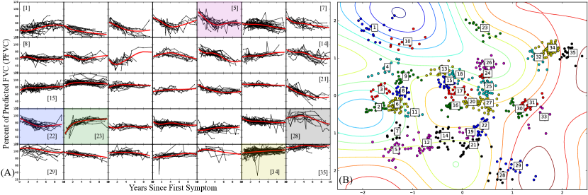
Figure 1: (A) Groups of PFVC trajectories obtained by hierarchical clustering of DTM representations. (B) Trajectory representations are color-coded and labeled according to groups shown in (A). Contours reflect posterior GP over the second B-spline coefficient (blue contours denote smaller values, red denote larger values).

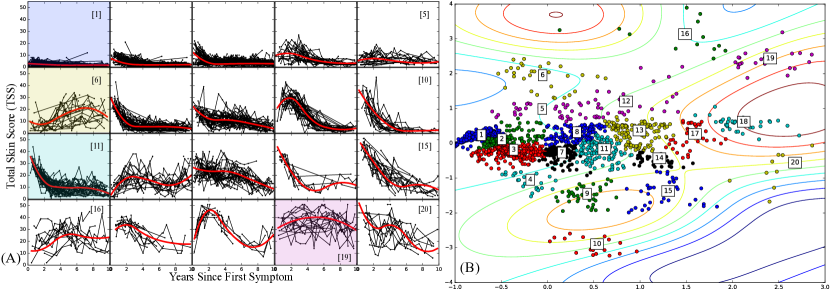
Figure 2: Same presentation as in Figure 1 but for TSS trajectories.

The DTM returns approximate posteriors over the representations $\bm{\mathrm{x}}_{i}$ for all individuals in the training set. We examine these posteriors for both the PFVC and TSS datasets to check for consistency with what is currently known about scleroderma disease trajectories. In Figure 1 (A) we show groups of trajectories uncovered by clustering the learned representations, which are plotted in Figure 1 (B). Many of the groups shown here align with other work on scleroderma lung disease subtypes (e.g. Schulam et al. (2015)). In particular, we see rapidly declining trajectories (group [5]), slowly declining trajectories (group [22]), recovering trajectories (group [23]), and stable trajectories (group [34]). Surprisingly, we also see a group of individuals who we describe as “late decliners” (group [28]). These individuals are stable for the first 5-6 years, but begin to decline thereafter. This is surprising because the onset of scleroderma-related lung disease is currently thought to occur early in the disease course (Varga et al., 2012). In Figure 2 (A) we show clusters of TSS trajectories and the corresponding color-coded representations in Figure 2 (B). These trajectories corroborate what is currently known about skin disease in scleroderma. In particular, we see individuals who have minimal activity (e.g. group [1]) and individuals with early activity that later stabilizes (e.g. group [11]), which correspond to what is known as the limited and diffuse variants of scleroderma (Varga et al., 2012). We also find that there are a number of individuals with increasing activity over time (group [6]) and some whose activity remains high over the ten year period (group [19]). These patterns are not currently considered to be canonical trajectories and warrant further investigation.

3.3 Associations between Representations and Clinical Outcomes

Table 1: Disease Trajectory Held-out Log-Likelihoods

	PFVC		TSS
Model	Subj. LL	Obs. LL	Subj. LL	Obs. LL
LMM	-17.59 ($\pm$ 1.18)	-3.95 ($\pm$ 0.04)	-13.63 ($\pm$ 1.41)	-3.47 ($\pm$ 0.05)
FPCA	-17.89 ($\pm$ 1.19)	-4.03 ($\pm$ 0.02)	-13.76 ($\pm$ 1.42)	-3.47 ($\pm$ 0.05)
DTM	-17.74 ($\pm$ 1.23)	-3.98 ($\pm$ 0.03)	-13.25 ($\pm$ 1.38)	-3.32 ($\pm$ 0.06)

Table 2: P-values under the null hypothesis that the distributions of trajectory representations are the same across individuals with and without clinical outcomes. Lower values indicate stronger support for rejection.

	PFVC			TSS
Outcome	LMM	FPCA	DTM	LMM	FPCA	DTM
Congestive Heart Failure	0.170	0.081	0.013	0.107	0.383	0.189
Pulmonary Hypertension	0.270	∗0.000	∗0.000	0.485	0.606	0.564
Pulmonary Arterial Hypertension	0.013	0.020	∗0.002	0.712	0.808	0.778
Gastrointestinal Complications	0.328	0.073	0.347	0.026	0.035	0.011
Myositis	0.337	∗0.002	∗0.004	∗0.000	∗0.002	∗0.000
Interstitial Lung Disease	∗0.000	∗0.000	∗0.000	0.553	0.515	0.495
Ulcers and Gangrene	0.410	0.714	0.514	0.573	0.316	∗0.009

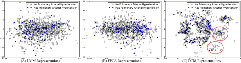
Figure 3: Scatter plots of representations for the three models color-coded by presence or absence of pulmonary arterial hypertension (PAH). Groups of trajectories with very few cases of PAH are circled in red.

To quantitatively evaluate the low-dimensional representations learned by the DTM, we statistically test for relationships between the representations of clinical marker trajectories and important clinical outcomes. We compare the inferences of the hypothesis test with those made using representations derived from the LMM and FPCA baselines. For the LMM, we project $\bm{\mathrm{w}}_{i}$ into its 2-dimensional principal subspace. For FPCA, we learn a rank-2 covariance, which recovers 2-dimensional embeddings. To establish that the models are all equally expressive and achieve comparable generalization error, we present held-out data log-likelihoods in Table 1, which are estimated using 10-fold cross-validation. We see that the models are roughly equivalent with respect to generalization error.

To test associations between clinical outcomes and learned representations, we use a kernel density estimator test (Duong et al., 2012) to test the null hypothesis that the distributions across subgroups with and without the outcome are equivalent. The $p$-values obtained are listed in Table 2. As a point of reference, we include two clinical outcomes that should be clearly related to the two clinical markers. Interstitial lung disease is the most common cause of lung damage in scleroderma (Varga et al., 2012), and so we confirm that the null hypothesis is rejected for all three models. Similarly, for TSS we expect ulcers and gangrene to be associated with severe skin disease. In this case, only the representations learned by DTM reveal this relationship. For the remaining outcomes, we see that FPCA and DTM reveal similar associations, but that only DTM suggests a relationship with pulmonary arterial hypertension (PAH). Presence of fibrosis (which drives lung disease progression) has been shown to be a risk factor in the development of PAH (see Chapter 36 of Varga et al. (2012)), but only the representations learned by DTM corroborate this finding (see Figure 3).

4 Conclusion

We present the Disease Trajectory Map (DTM), a novel probabilistic model that learns low-dimensional embeddings of sparse and irregularly sampled clinical time series data. The DTM is a reformulation of the LMM that places an emphasis on the representations that the model learns. This view is comparable to that taken by Lawrence (2004) in deriving the Gaussian process latent variable model (GPLVM) from probabilistic principal component analysis (PPCA) (Tipping and Bishop, 1999), and indeed the DTM can be interpreted as a “twin kernel” GPLVM (briefly discussed in the concluding paragraphs) over functional observations. The DTM can also be viewed as an LMM with a “warped” Gaussian prior over the random effects (see e.g. Damianou et al. (2015) for a discussion of distributions induced by mapping Gaussian random variables through non-linear maps). We demonstrate the model by analyzing data extracted from one of the nation’s largest scleroderma patient registries, and found that the DTM induces structure among trajectories that is consistent with previous findings and also uncovers several surprising disease trajectory shapes. We also explore associations between important clinical outcomes and the DTM’s representations and found statistically significant differences in representations between outcome-defined groups that were not uncovered by two sets of baseline representations.

Appendix A Derivation of Evidence Lower Bound

When marginalizing over the rows of $\mathrm{F}$, we induced a Gaussian process over the trajectories, but by doing so we implicitly induced a Gaussian process over the subject-specific basis coefficients. Let $\bm{\mathrm{w}}_{i}\triangleq\mathrm{F}\bm{\mathrm{x}}_{i}\in\mathbb{R}^{d}$ denote the curve weights implied by the mapping $\mathrm{F}$ and representation $\bm{\mathrm{x}}_{i}$, and let $\bm{\mathrm{w}}_{:,k}$ for $k\in[d]$ denote the $k^{\text{th}}$ coefficient of all subjects in the dataset. After marginalizing the $k^{\text{th}}$ row of $\mathrm{F}$ and applying the kernel trick, we see that the vector of coefficients $\bm{\mathrm{w}}_{:,k}$ has a Gaussian process distribution with mean $0$ and covariance

$$\operatorname{Cov}(w_{ik},w_{jk})=\alpha k(\bm{\mathrm{x}}_{i},\bm{\mathrm{x}}_{j}).$$ (14)

Moreover, the Gaussian processes across coefficients are mutually statistically independent of one another. To construct our approximate objective, we first approximate each of the $d$ coefficient Gaussian processes by introducing $p$ inducing points (see e.g. Snelson and Ghahramani (2005); Titsias (2009)) with values $\bm{\mathrm{u}}_{k}\in\mathbb{R}^{p}$ for each $k\in[d]$ observed at common inputs $\bm{\mathrm{z}}_{i}\in\mathbb{R}^{q}$ for $i\in[p]$. We assume that each $\bm{\mathrm{w}}_{:,k}$ and $\bm{\mathrm{u}}_{k}$ are sampled from a common Gaussian process, which implies the joint distribution:

$$\bm{\mathrm{u}}_{k} \mid\bm{\mathrm{\theta}}\sim\mathcal{N}(\bm{\mathrm{0}},\mathrm{K}_{pp})$$ (15)

$$\bm{\mathrm{w}}_{k} \mid\bm{\mathrm{u}}_{k},\bm{\mathrm{\theta}}\sim\mathcal{N}(\mathrm{K}_{mp}\mathrm{K}^{{-1}}_{pp}\bm{\mathrm{u}}_{k},\tilde{\mathrm{K}}_{mm}).$$ (16)

where $\mathrm{K}_{pp}$ is the Gram matrix between inducing points, $\mathrm{K}_{mm}$ is the Gram matrix between subjects (based on their representations $\bm{\mathrm{x}}_{i}$), $\mathrm{K}_{mp}$ is the cross Gram matrix between subjects and inducing points, and $\tilde{\mathrm{K}}_{mm}\triangleq\mathrm{K}_{mm}-\mathrm{K}_{mp}\mathrm{K}^{{-1}}_{pp}\mathrm{K}_{pm}$.

Now, we stack the inducing point values $\bm{\mathrm{u}}_{1:d}$ into the columns of a matrix $\mathrm{U}\triangleq[\bm{\mathrm{u}}_{1},\ldots,\bm{\mathrm{u}}_{d}]$. We will use $\bm{\mathrm{u}}$ to denote the “vectorization” of $\mathrm{U}$ obtained by stacking the columns. Each row $i$ of $\mathrm{U}$ can be thought of as the vector of coefficients belonging to a single inducing subject which has an associated representation $\bm{\mathrm{z}}_{i}\in\mathbb{R}^{q}$. Let $\bm{\mathrm{y}}\triangleq[\bm{\mathrm{y}}^{\top}_{1},\ldots,\bm{\mathrm{y}}^{\top}_{m}]^{\top}$ be the vector of concatenated trajectories and $\mathrm{W}$ be the matrix containing subject $i$’s coefficients $\bm{\mathrm{w}}_{i}$ in each row, then following the derivation of Hensman et al. (2013), we can lower bound the conditional log-probability of $\bm{\mathrm{y}}$ given $\bm{\mathrm{u}}$ and $\bm{\mathrm{x}}_{1:m}$:

$$\log p(\bm{\mathrm{y}}\mid\bm{\mathrm{u}},\bm{\mathrm{x}}_{1:m}) =\log\int p(\bm{\mathrm{y}}\mid\mathrm{W})p(\mathrm{W}\mid\bm{\mathrm{u}},\bm{\mathrm{x}}_{1:m})d\mathrm{W}$$ (17)

$$=\log\int\prod_{i=1}^{m}p(\bm{\mathrm{y}}_{i}\mid\bm{\mathrm{w}}_{i})p(\mathrm{W}\mid\bm{\mathrm{u}},\bm{\mathrm{x}}_{1:m})d\mathrm{W}$$ (18)

$$\geq\int p(\mathrm{W}\mid\bm{\mathrm{u}},\bm{\mathrm{x}}_{1:m})\sum_{i=1}^{m}\log p(\bm{\mathrm{y}}_{i}\mid\bm{\mathrm{w}}_{i})d\mathrm{W}$$ (19)

$$=\sum_{i=1}^{m}\mathbb{E}_{p(\bm{\mathrm{w}}_{i}\mid\bm{\mathrm{u}},\bm{\mathrm{x}}_{i})}[\log p(\bm{\mathrm{y}}_{i}\mid\bm{\mathrm{w}}_{i})].$$ (20)

The expectation in each summand is easy to calculate because the mean of $\bm{\mathrm{y}}_{i}$ is linearly dependent on $\bm{\mathrm{w}}_{i}$ and because the conditional distribution $\bm{\mathrm{w}}_{i}$ given $\bm{\mathrm{u}}$ is multivariate normal. Specifically, we have that

$$\bm{\mathrm{w}}_{i}\mid\bm{\mathrm{u}},\bm{\mathrm{x}}_{i}\sim\mathcal{N}(\mathrm{U}^{\top}\mathrm{K}^{{-1}}_{pp}\bm{\mathrm{k}}_{i},\tilde{k}_{ii}\mathrm{I}_{d}),$$ (21)

where $\bm{\mathrm{k}}_{i}$ is a column vector filled with the $i^{\text{th}}$ row of $\mathrm{K}_{mp}$ and $\tilde{k}_{ii}$ is the $i^{\text{th}}$ diagonal element of $\tilde{\mathrm{K}}_{mm}$. Together with the conditional distribution of $\bm{\mathrm{y}}_{i}$ given $\bm{\mathrm{w}}_{i}$, we have that each summand can be written as

$$\mathbb{E}_{p(\bm{\mathrm{w}}_{i}\mid\bm{\mathrm{u}},\bm{\mathrm{x}}_{i})}[\log p(\bm{\mathrm{y}}_{i}\mid\bm{\mathrm{w}}_{i})]$$ (22)

$$=-\frac{n_{i}}{2}\log 2\pi\sigma^{2}-\frac{1}{2\sigma^{2}}\mathbb{E}_{p(\bm{\mathrm{w}}_{i}\mid\bm{\mathrm{u}},\bm{\mathrm{x}}_{i})}[(\bm{\mathrm{y}}_{i}-\mu-\mathrm{B}_{i}\bm{\mathrm{w}}_{i})^{\top}(\bm{\mathrm{y}}_{i}-\mu-\mathrm{B}_{i}\bm{\mathrm{w}}_{i})]$$ (23)

$$=\log\mathcal{N}(\bm{\mathrm{y}}_{i}\mid\mu+\mathrm{B}_{i}\mathrm{U}^{\top}\mathrm{K}^{{-1}}_{pp}\bm{\mathrm{k}}_{i},\sigma^{2}\mathrm{I}_{n_{i}})-\frac{\tilde{k}_{ii}}{2\sigma^{2}}\operatorname{Tr}[\mathrm{B}^{\top}_{i}\mathrm{B}_{i}]$$ (24)

$$\triangleq\log\tilde{p}(\bm{\mathrm{y}}_{i}\mid\bm{\mathrm{u}},\bm{\mathrm{x}}_{i}).$$ (25)

We can now write the lower bound on the conditional log-probability as

$$\log p(\bm{\mathrm{y}}\mid\bm{\mathrm{u}},\bm{\mathrm{x}}_{1:m})\geq\sum_{i=1}^{m}\log\tilde{p}(\bm{\mathrm{y}}_{i}\mid\bm{\mathrm{u}},\bm{\mathrm{x}}_{i})\triangleq\log\tilde{p}(\bm{\mathrm{y}}\mid\bm{\mathrm{u}},\bm{\mathrm{x}}_{1:m}).$$ (26)

To complete the derivation of the approximate objective, we use the lower bound on $\log p(\bm{\mathrm{y}}\mid\bm{\mathrm{u}},\bm{\mathrm{x}}_{1:m})$ to create a variational lower bound on the marginal log-probability of the trajectories

$$\log p(\bm{\mathrm{y}}) =\log\int p(\bm{\mathrm{y}}\mid\bm{\mathrm{u}},\bm{\mathrm{x}}_{1:m})p(\bm{\mathrm{u}},\bm{\mathrm{x}}_{1:m})d\bm{\mathrm{u}}$$ (27)

$$\geq\int q(\bm{\mathrm{u}},\bm{\mathrm{x}}_{1:m})\left(\log p(\bm{\mathrm{y}}\mid\bm{\mathrm{u}},\bm{\mathrm{x}}_{1:m})-\log q(\bm{\mathrm{u}},\bm{\mathrm{x}}_{1:m})+\log p(\bm{\mathrm{u}},\bm{\mathrm{x}}_{1:m})\right)d\bm{\mathrm{u}}d\bm{\mathrm{x}}_{1:m}$$ (28)

$$\geq\int q(\bm{\mathrm{u}},\bm{\mathrm{x}}_{1:m})\left(\log\tilde{p}(\bm{\mathrm{y}}\mid\bm{\mathrm{u}},\bm{\mathrm{x}}_{1:m})-\log q(\bm{\mathrm{u}},\bm{\mathrm{x}}_{1:m})+\log p(\bm{\mathrm{u}},\bm{\mathrm{x}}_{1:m})\right)d\bm{\mathrm{u}}d\bm{\mathrm{x}}_{1:m}$$ (29)

$$\triangleq\log\tilde{p}(\bm{\mathrm{y}}).$$ (30)

We assume that $\bm{\mathrm{u}}$, $\bm{\mathrm{x}}_{1},\ldots,\bm{\mathrm{x}}_{m}$ are all mutually independent in the variational posterior. We use a multivariate normal variational approximation for each $\bm{\mathrm{x}}_{i}$ with variational parameters $\bm{\mathrm{m}}_{i}$ and $\mathrm{S}_{i}$.

Fixing $\bm{\mathrm{x}}_{i}$, to find the the optimal form for $q(\bm{\mathrm{u}})$, note that each $\log\tilde{p}(\bm{\mathrm{y}}_{i}\mid\bm{\mathrm{u}},\bm{\mathrm{x}}_{i})$ is composed of a log-likelihood plus an additive term that is independent of $\bm{\mathrm{u}}$. Therefore, the terms that depend on $\bm{\mathrm{u}}$ can be written as:

$$\mathbb{E}_{q(\bm{\mathrm{u}})}\left[\sum_{i=1}^{m}\log\mathcal{N}(\bm{\mathrm{y}}_{i}\mid\mu+\mathrm{B}_{i}\mathrm{U}^{\top}\mathrm{K}^{{-1}}_{pp}\bm{\mathrm{k}}_{i},\sigma^{2}\mathrm{I}_{n_{i}})\right]-\operatorname{KL}(q\|p).$$ (31)

Now, note that the mean in any of the log-likelihood terms can be rewritten as

$$\mu+\mathrm{B}_{i}\mathrm{U}^{\top}\mathrm{K}^{{-1}}_{pp}\bm{\mathrm{k}}_{i}=\mu+(\mathrm{B}_{i}\otimes\bm{\mathrm{k}}^{\top}_{i}\mathrm{K}^{{-1}}_{pp})\bm{\mathrm{u}},$$ (32)

Let $\mathrm{C}_{i}\triangleq(\mathrm{B}_{i}\otimes\bm{\mathrm{k}}^{\top}_{i}\mathrm{K}^{{-1}}_{pp})$ denote the extended design matrix obtained through this rewriting, and recall that each column $\bm{\mathrm{u}}_{k}$ is normally distributed with mean zero and covariance $\mathrm{K}_{pp}$. The prior over the vectorized matrix $\bm{\mathrm{u}}$ is therefore also multivariate normal. The expression above is maximized when $q(\bm{\mathrm{u}})$ is equal to the posterior over $\bm{\mathrm{u}}$ given the observed trajectories. Because the prior is multivariate normal and the mean of the likelihood depends linearly on $\bm{\mathrm{u}}$, the posterior must also be multivariate normal. Moreover, we know its exact form:

$$\bm{\mathrm{m}}_{*}=\mathrm{S}_{*}\left(\sigma^{-2}\sum_{i=1}^{m}\mathrm{C}^{\top}_{i}(\bm{\mathrm{y}}_{i}-\mu)\right)\,\,\,,\,\,\,\mathrm{S}_{*}=\left(\sigma^{-2}\sum_{i=1}^{m}\mathrm{C}^{\top}_{i}\mathrm{C}_{i}+(\mathrm{I}_{d}\otimes\mathrm{K}^{{-1}}_{pp})\right)^{{-1}}.$$ (33)

We therefore parameterize $q(\bm{\mathrm{u}})$ as a multivariate normal distribution with variational parameters $\bm{\mathrm{m}}$ and $\mathrm{S}$.

We now derive a closed-form expression for the expectation of $\log\tilde{p}(\bm{\mathrm{y}}_{i}\mid\bm{\mathrm{u}},\bm{\mathrm{x}}_{i})$ under variational posterior distribution. Because $\bm{\mathrm{u}}$ and $\bm{\mathrm{x}}_{i}$ are assumed to be independent in the variational posteriors, we can analyze the expectation in either order. Fix $\bm{\mathrm{x}}_{i}$, then we see that $\log\tilde{p}(\bm{\mathrm{y}}_{i}\mid\bm{\mathrm{u}},\bm{\mathrm{x}}_{i})$ depends on $\bm{\mathrm{u}}$ only through the mean of the Gaussian density, which is a quadratic term in log likelihood. Because $q(\bm{\mathrm{u}})$ is multivariate normal, we can compute the expectation in closed form.

$$\mathbb{E}_{q(\bm{\mathrm{u}})}[\log\tilde{p}(\bm{\mathrm{y}}_{i}\mid\bm{\mathrm{u}},\bm{\mathrm{x}}_{i})] =\mathbb{E}_{q(\mathrm{U})}[\log\mathcal{N}(\bm{\mathrm{y}}_{i}\mid\mu+(\mathrm{B}_{i}\otimes\bm{\mathrm{k}}^{\top}_{i}\mathrm{K}^{{-1}}_{pp})\bm{\mathrm{u}},\sigma^{2}\mathrm{I}_{n_{i}})]-\frac{\tilde{k}_{ii}}{2\sigma^{2}}\operatorname{Tr}[\mathrm{B}^{\top}_{i}\mathrm{B}_{i}]$$

$$=\log\mathcal{N}(\bm{\mathrm{y}}_{i}\mid\mu+\mathrm{C}_{i}\bm{\mathrm{m}},\sigma^{2}\mathrm{I}_{n_{i}})]-\frac{1}{2\sigma^{2}}\operatorname{Tr}[\mathrm{S}\mathrm{C}^{\top}_{i}\mathrm{C}_{i}]-\frac{\tilde{k}_{ii}}{2\sigma^{2}}\operatorname{Tr}[\mathrm{B}^{\top}_{i}\mathrm{B}_{i}],$$

We can compute the expectation of $\mathbb{E}_{q(\bm{\mathrm{u}})}[\log\tilde{p}(\bm{\mathrm{y}}_{i}\mid\bm{\mathrm{u}},\bm{\mathrm{x}}_{i})]$ in closed form by noting that we need only compute expectations of $\bm{\mathrm{k}}_{i}$ and $\bm{\mathrm{k}}_{i}\bm{\mathrm{k}}^{\top}_{i}$. Specifically, we have that

$$\mathbb{E}_{q(\bm{\mathrm{x}}_{i})}[k(\bm{\mathrm{x}}_{i},\bm{\mathrm{z}}_{j})]=\frac{\alpha}{|\mathrm{S}_{i}|^{1/2}|\mathrm{A}|^{1/2}}\exp\left\{\frac{1}{2}(\bm{\mathrm{B}}^{\top}\mathrm{A}^{{-1}}\bm{\mathrm{b}}-c)\right\},$$ (34)

where $\mathrm{A}=\mathrm{S}^{{-1}}_{i}+\ell^{-2}\mathrm{I}_{q}$, $\bm{\mathrm{b}}=\mathrm{S}^{{-1}}_{i}\bm{\mathrm{m}}_{i}+\ell^{-2}\bm{\mathrm{z}}_{j}$, and $c=\bm{\mathrm{m}}^{\top}_{i}\mathrm{S}^{{-1}}_{i}\bm{\mathrm{m}}+\ell^{-2}\bm{\mathrm{z}}^{\top}_{j}\bm{\mathrm{z}}_{j}$. Similarly, for the expected outer product, we have

$$\mathbb{E}_{q(\bm{\mathrm{x}}_{i})}[k(\bm{\mathrm{x}}_{i},\bm{\mathrm{z}}_{j})k(\bm{\mathrm{x}}_{i},\bm{\mathrm{z}}_{k})]=\frac{\alpha}{|\mathrm{S}_{i}|^{1/2}|\mathrm{A}|^{1/2}}\exp\left\{\frac{1}{2}(\bm{\mathrm{B}}^{\top}\mathrm{A}^{{-1}}\bm{\mathrm{b}}-c)\right\},$$ (35)

where $\mathrm{A}=\mathrm{S}^{{-1}}_{i}+2\ell^{-2}\mathrm{I}_{q}$, $\bm{\mathrm{b}}=\mathrm{S}^{{-1}}_{i}\bm{\mathrm{m}}_{i}+\ell^{-2}\bm{\mathrm{z}}_{j}+\ell^{-2}\bm{\mathrm{z}}_{k}$, and $c=\bm{\mathrm{m}}^{\top}_{i}\mathrm{S}^{{-1}}_{i}\bm{\mathrm{m}}+\ell^{-2}\bm{\mathrm{z}}^{\top}_{j}\bm{\mathrm{z}}_{j}+\ell^{-2}\bm{\mathrm{z}}^{\top}_{k}\bm{\mathrm{z}}_{k}$. Importantly, we can simply substitute these expectations into $\mathbb{E}_{q(\bm{\mathrm{u}})}[\log\tilde{p}(\bm{\mathrm{y}}_{i}\mid\bm{\mathrm{u}},\bm{\mathrm{x}}_{i})]$ and the form of the lower bound does not change (it is still a Gaussian log-likelihood plus the additional trace terms).

Appendix B Optimizing the Evidence Lower Bound

To formulate the complete objective, we use the lower bound derived above and place priors on the observation noise $\sigma^{2}$, and the hyperparameters of the kernel $k(\cdot,\cdot)$. In this section and in our experiments we assume that the kernel is a radial basis function (RBF) with scale $\alpha$ and length-scale (or bandwidth) $\ell$. We assumelog normal distributions over $\sigma^{2}$, $\alpha$, and $\ell$ with mean parameters $m_{s}$, $m_{a}$, $m_{\ell}$ respectively and precision parameters $\rho_{s}$, $\rho_{a}$, and $\rho_{\ell}$ respectively. Our objective is therefore

$$\mathcal{J}_{\text{SA-DTM}}( \bm{\mathrm{m}},\mathrm{S},\bm{\mathrm{m}}_{1:m},\mathrm{S}_{1:m},\mu,\sigma^{2},\alpha,\ell)=$$ (36)

$$\phantom{{}+{}}\sum_{i=1}^{m}-\frac{n_{i}}{2}\log 2\pi\sigma^{2}-\frac{1}{2\sigma^{2}}\mathbb{E}_{q(\bm{\mathrm{x}}_{i})}[\|\bm{\mathrm{y}}_{i}-\mu-(\mathrm{B}_{i}\otimes\bm{\mathrm{k}}^{\top}_{i}\mathrm{K}^{{-1}}_{pp})\bm{\mathrm{m}}\|_{2}^{2}]$$ (37)

$$+\sum_{i=1}^{m}-\frac{1}{2\sigma^{2}}\operatorname{Tr}[\mathrm{S}(\mathrm{B}^{\top}_{i}\mathrm{B}_{i}\otimes\mathrm{K}^{{-1}}_{pp}\mathbb{E}_{q(\bm{\mathrm{x}}_{i})}[\bm{\mathrm{k}}_{i}\bm{\mathrm{k}}^{\top}_{i}]\mathrm{K}^{{-1}}_{pp})]$$ (38)

$$+\sum_{i=1}^{m}-\frac{1}{2\sigma^{2}}\operatorname{Tr}[\mathrm{B}^{\top}_{i}\mathrm{B}_{i}](\alpha-\mathbb{E}_{q(\bm{\mathrm{x}}_{i})}[\bm{\mathrm{k}}^{\top}_{i}\mathrm{K}^{{-1}}_{pp}\bm{\mathrm{k}}_{i}])$$ (39)

$$-\sum_{i=1}^{m}\frac{1}{2}\left(\operatorname{Tr}[\mathrm{S}_{i}+\bm{\mathrm{m}}_{i}\bm{\mathrm{m}}^{\top}_{i}]-q-\log|\mathrm{S}_{i}|\right)$$ (40)

$$-\frac{1}{2}\left(\operatorname{Tr}[(\mathrm{S}+\bm{\mathrm{m}}\bm{\mathrm{m}}^{\top})(\mathrm{I}_{d}\otimes\mathrm{K}^{{-1}}_{pp})]-pd+\log\frac{|\mathrm{K}_{pp}|^{d}}{|\mathrm{S}|}\right)$$ (41)

$$-\frac{\rho_{s}}{2}\|\log\sigma^{2}-m_{s}\|^{2}_{2}-\frac{\rho_{a}}{2}\|\log\alpha-m_{a}\|^{2}_{2}-\frac{\rho_{\ell}}{2}\|\log\ell-m_{\ell}\|^{2}_{2}.$$ (42)

Note that the last three lines above can be seen as regularizers (log priors for the hyperparameters and a $\operatorname{KL}$ divergence between the variational distribution $q$ and the prior $p$). The first four lines can be decomposed across subjects, suggesting that we can use stochastic approximation of the objective and its gradients to derive a scalable algorithm for optimizing the objective.

We define an iterative first-order optimization algorithm. In broad strokes, within each iteration we will sample a single subject $i$ (or a batch of patients), maximize the objective with respect to $\bm{\mathrm{m}}_{i}$ and $\mathrm{S}_{i}$ while holding the global variables fixed, compute the approximate gradients of the objective, and take a small step in the direction of each gradient for each parameter (the step size is determined by a learning schedule, which may be specific to each global variable). We discuss each step in detail below. We do so assuming a single sampled subject $i$, although in principle we can sample a batch of subjects to reduce variance in the gradient estimate.

Maximizing wrt local variables ($\bm{\mathrm{m}}_{i},\mathrm{S}_{i}$).

Before computing gradients of the approximate objective with respect to the global parameters, we first do a block coordinate optimization over the local variational parameters of subject $i$. We optimize:

$$J_{i} (\bm{\mathrm{x}}_{i})=$$ (43)

$$-\frac{n_{i}}{2}\log 2\pi\sigma^{2}-\frac{1}{2\sigma^{2}}\mathbb{E}_{q(\bm{\mathrm{x_{i}}})}[\|\bm{\mathrm{y}}_{i}-\mu-(\mathrm{B}_{i}\otimes\bm{\mathrm{k}}^{\top}_{i}\mathrm{K}^{{-1}}_{pp})\bm{\mathrm{m}}\|^{2}_{2}]$$ (44)

$$-\frac{1}{2\sigma^{2}}\operatorname{Tr}[\mathrm{S}(\mathrm{B}^{\top}_{i}\mathrm{B}_{i}\otimes\mathrm{K}^{{-1}}_{pp}\mathbb{E}_{q(\bm{\mathrm{x_{i}}})}[\bm{\mathrm{k}}_{i}\bm{\mathrm{k}}^{\top}_{i}]\mathrm{K}^{{-1}}_{pp})]$$ (45)

$$-\frac{1}{2\sigma^{2}}\operatorname{Tr}[\mathrm{B}^{\top}_{i}\mathrm{B}_{i}](\alpha-\mathbb{E}_{q(\bm{\mathrm{x_{i}}})}[\bm{\mathrm{k}}^{\top}_{i}\mathrm{K}^{{-1}}_{pp}\bm{\mathrm{k}}_{i}]).$$ (46)

We can optimize this expression using a gradient-based optimizer. We use the scaled conjugate gradients algorithm.

Estimating gradients of global variables.

Having sampled subject $i$ and refit her local variational parameters, we now want to approximate the gradient of the full objective with respect to the global variables $\bm{\mathrm{m}}$, $\mathrm{S}$, $\mu$, $\sigma^{2}$, $\alpha$, and $\ell$. We first look at the approximate gradient with respect to $\bm{\mathrm{m}}$.

$$\hat{\nabla}_{\mathcal{J}_{\text{SA-DTM}}}(\bm{\mathrm{m}})=\mathbb{E}_{q(\bm{\mathrm{x}}_{i})}[\frac{m}{\sigma^{2}}(\mathrm{B}^{\top}_{i}\otimes\mathrm{K}^{{-1}}_{pp}\bm{\mathrm{k}}_{i})(\bm{\mathrm{y}}_{i}-\mu-(\mathrm{B}\otimes\bm{\mathrm{k}}^{\top}_{i}\mathrm{K}^{{-1}}_{pp})\bm{\mathrm{m}})]-(\mathrm{I}_{d}\otimes\mathrm{K}^{{-1}}_{pp})\bm{\mathrm{m}}.$$ (47)

The approximate gradient with respect to $\mathrm{S}$ is

$$\hat{\nabla}_{\mathcal{J}_{\text{SA-DTM}}}(\mathrm{S})= -\frac{m}{2\sigma^{2}}\operatorname{Tr}[(\mathrm{B}^{\top}_{i}\mathrm{B}_{i}\otimes\mathrm{K}^{{-1}}_{pp}\mathbb{E}_{q(\bm{\mathrm{x}}_{i})}[\bm{\mathrm{k}}_{i}\bm{\mathrm{k}}^{\top}_{i}]\mathrm{K}^{{-1}}_{pp})]$$ (48)

$$-\frac{1}{2}\operatorname{Tr}[(\mathrm{I}_{d}\otimes\mathrm{K}^{{-1}}_{pp})]+\frac{1}{2}\operatorname{Tr}[\mathrm{S}^{{-1}}].$$ (49)

Note that if we set these approximate gradients to $0$, we obtain the following estimates of $\bm{\mathrm{m}}$ and $\mathrm{S}$:

$$\hat{\bm{\mathrm{m}}} =\hat{\mathrm{S}}\left(\frac{m}{\sigma^{2}}(\mathrm{B}^{\top}_{i}\otimes\mathrm{K}^{{-1}}_{pp}\mathbb{E}_{q(\bm{\mathrm{x}}_{i})}[\bm{\mathrm{k}}_{i}])(\bm{\mathrm{y}}-\mu)\right)$$ (50)

$$\hat{\mathrm{S}} =\left(\frac{m}{\sigma^{2}}(\mathrm{B}^{\top}_{i}\mathrm{B}_{i}\otimes\mathrm{K}^{{-1}}_{pp}\mathbb{E}_{q(\bm{\mathrm{x}}_{i})}[\bm{\mathrm{k}}_{i}\bm{\mathrm{k}}^{\top}_{i}]\mathrm{K}^{{-1}}_{pp})+(\mathrm{I}_{d}\otimes\mathrm{K}^{{-1}}_{pp})\right)^{-1}$$ (51)

We can improve the rate of convergence of our algorithm by taking the geometry of the space of distributions parameterized by $\bm{\mathrm{m}}$ and $\mathrm{S}$ into account. We do so by using the natural gradients for these two parameters instead of the approximations above. Let $\bm{\mathrm{\theta}}_{1}$ and $\mathrm{\theta}_{2}$ denote the canonical parameterization of the variational multivariate normal, then the gradient updates at time $t$ are Hoffman et al. (2013):

$$\bm{\mathrm{\theta}}_{1}^{t} =\bm{\mathrm{\theta}}_{1}^{t-1}+\lambda_{t}(\eta_{1}^{t-1}-\bm{\mathrm{\theta}}_{1}^{t-1})$$ (52)

$$\mathrm{\theta}_{2}^{t} =\mathrm{\theta}_{2}^{t-1}+\lambda_{t}(\eta_{2}^{t-1}-\mathrm{\theta}_{2}^{t-1}),$$ (53)

where

$$\eta_{1}^{t-1} =\frac{m}{\sigma^{2}}(\mathrm{B}^{\top}_{i}\otimes\mathrm{K}^{{-1}}_{pp}\mathbb{E}_{q(\bm{\mathrm{x}}_{i})}[\bm{\mathrm{k}}_{i}])(\bm{\mathrm{y}}-\mu)$$ (54)

$$\eta_{2}^{t-1} =-\frac{m}{2\sigma^{2}}(\mathrm{B}^{\top}_{i}\mathrm{B}_{i}\otimes\mathrm{K}^{{-1}}_{pp}\mathbb{E}_{q(\bm{\mathrm{x}}_{i})}[\bm{\mathrm{k}}_{i}\bm{\mathrm{k}}^{\top}_{i}]\mathrm{K}^{{-1}}_{pp})$$ (55)

To update the hyperparamters, we need to compute the gradients with respect to $\mu$, $\sigma^{2}$, $\alpha$, and $\ell$. We parameterize $\sigma^{2}$, $\alpha$, and $\ell$ using their logarithms, and so present gradients with respect to that representation. To make the expressions more clear, we present the gradients as differentials with respect to the kernel, which can be completed using the chain rule. The estimate of the gradient with respect to $\mu$ is

$$\hat{\nabla}_{\mathcal{J}_{\text{SA-DTM}}}(\mu)=\frac{m}{\sigma^{2}}(\bm{\mathrm{y}}_{i}-\mu-(\mathrm{B}_{i}\otimes\mathbb{E}_{q(\bm{\mathrm{x}}_{i})}[\bm{\mathrm{k}}^{\top}_{i}]{}\mathrm{K}^{{-1}}_{pp})\bm{\mathrm{m}})^{\top}\bm{\mathrm{1}}_{n_{i}}.$$ (56)

The estimate of the gradient with respect to $\log\sigma^{2}$ is

$$\hat{\nabla}_{\mathcal{J}_{\text{SA-DTM}}}(\log\sigma^{2})= -\frac{mn_{i}}{2}+\frac{m}{2\sigma^{2}}\mathbb{E}_{q(\bm{\mathrm{x}}_{i})}[\|\bm{\mathrm{y}}_{i}-\mu-(\mathrm{B}_{i}\otimes\bm{\mathrm{k}}^{\top}_{i}\mathrm{K}^{{-1}}_{pp})\bm{\mathrm{m}}\|^{2}_{2}]$$ (57)

$$+\frac{m}{2\sigma^{2}}\operatorname{Tr}[\mathrm{S}(\mathrm{B}^{\top}_{i}\mathrm{B}_{i}\otimes\mathrm{K}^{{-1}}_{pp}\mathbb{E}_{q(\bm{\mathrm{x}}_{i})}[\bm{\mathrm{k}}_{i}\bm{\mathrm{x}}^{\top}_{i}]{}\mathrm{K}^{{-1}}_{pp})]$$ (58)

$$+\frac{m}{2\sigma^{2}}\operatorname{Tr}[\mathrm{B}^{\top}_{i}\mathrm{B}](\alpha-\operatorname{Tr}[\mathrm{K}^{{-1}}_{pp}\mathbb{E}_{q(\bm{\mathrm{x}}_{i})}[\bm{\mathrm{k}}_{i}\bm{\mathrm{x}}^{\top}_{i}]{}])$$ (59)

$$-\rho_{s}(\log\sigma^{2}-m_{s}).$$ (60)

The estimate of the gradient with respect to $\log\alpha$ is

$$\hat{\nabla}_{\text{SA-DTM}} (\log\alpha)=$$ (61)

$$\phantom{{}+{}}\frac{m}{\sigma^{2}}\mathbb{E}_{q(\bm{\mathrm{x}}_{i})}[(\bm{\mathrm{y}}_{i}-\mu-\mathrm{C}\bm{\mathrm{m}})^{\top}(\mathrm{B}_{i}\otimes\partial\bm{\mathrm{k}}^{\top}_{i}\mathrm{K}^{{-1}}_{pp}-\bm{\mathrm{k}}^{\top}_{i}\mathrm{K}^{{-1}}_{pp}\partial\mathrm{K}_{pp}\mathrm{K}^{{-1}}_{pp})\bm{\mathrm{m}}]$$ (62)

$$-\frac{m}{\sigma^{2}}\mathbb{E}_{q(\bm{\mathrm{x}}_{i})}[\operatorname{Tr}[\mathrm{S}\mathrm{C}^{\top}_{i}(\mathrm{B}_{i}\otimes\partial\bm{\mathrm{k}}^{\top}_{i}\mathrm{K}^{{-1}}_{pp}-\bm{\mathrm{k}}^{\top}_{i}\mathrm{K}^{{-1}}_{pp}\partial\mathrm{K}_{pp}\mathrm{K}^{{-1}}_{pp})]]$$ (63)

$$-\frac{m}{2\sigma^{2}}\operatorname{Tr}[\mathrm{B}^{\top}_{i}\mathrm{B}_{i}]\alpha$$ (64)

$$+\frac{m}{2\sigma^{2}}\operatorname{Tr}[\mathrm{B}^{\top}_{i}\mathrm{B}_{i}](2\mathbb{E}_{q(\bm{\mathrm{x}}_{i})}[\bm{\mathrm{k}}^{\top}_{i}]{}\mathrm{K}^{{-1}}_{pp}\partial\mathbb{E}_{q(\bm{\mathrm{x}}_{i})}[\bm{\mathrm{k}}_{i}]{}-\operatorname{Tr}[\mathrm{K}^{{-1}}_{pp}\partial\mathrm{K}_{pp}\mathrm{K}^{{-1}}_{pp}\mathbb{E}_{q(\bm{\mathrm{x}}_{i})}[\bm{\mathrm{k}}_{i}\bm{\mathrm{x}}^{\top}_{i}]{}])$$ (65)

$$+\frac{1}{2}\left(\operatorname{Tr}[(\mathrm{S}+\mathrm{m}\mathrm{m}^{\top})(\mathrm{I}_{d}\otimes\mathrm{K}^{{-1}}_{pp}\partial\mathrm{K}_{pp}\mathrm{K}^{{-1}}_{pp})]-d\operatorname{Tr}[\mathrm{K}^{{-1}}_{pp}\partial\mathrm{K}_{pp}]\right).$$ (66)

The estimate of the gradient with respect to $\log\ell$ is

$$\hat{\nabla}_{\text{SA-DTM}} (\log\ell)=$$ (67)

$$\phantom{{}+{}}\frac{m}{\sigma^{2}}\mathbb{E}_{q(\bm{\mathrm{x}}_{i})}[(\bm{\mathrm{y}}_{i}-\mu-\mathrm{C}\bm{\mathrm{m}})^{\top}(\mathrm{B}_{i}\otimes\partial\bm{\mathrm{k}}^{\top}_{i}\mathrm{K}^{{-1}}_{pp}-\bm{\mathrm{k}}^{\top}_{i}\mathrm{K}^{{-1}}_{pp}\partial\mathrm{K}_{pp}\mathrm{K}^{{-1}}_{pp})\bm{\mathrm{m}}]$$ (68)

$$-\frac{m}{\sigma^{2}}\mathbb{E}_{q(\bm{\mathrm{x}}_{i})}[\operatorname{Tr}[\mathrm{S}\mathrm{C}^{\top}_{i}(\mathrm{B}_{i}\otimes\partial\bm{\mathrm{k}}^{\top}_{i}\mathrm{K}^{{-1}}_{pp}-\bm{\mathrm{k}}^{\top}_{i}\mathrm{K}^{{-1}}_{pp}\partial\mathrm{K}_{pp}\mathrm{K}^{{-1}}_{pp})]]$$ (69)

$$+\frac{m}{2\sigma^{2}}\operatorname{Tr}[\mathrm{B}^{\top}_{i}\mathrm{B}_{i}](2\mathbb{E}_{q(\bm{\mathrm{x}}_{i})}[\bm{\mathrm{k}}^{\top}_{i}]{}\mathrm{K}^{{-1}}_{pp}\partial\mathbb{E}_{q(\bm{\mathrm{x}}_{i})}[\bm{\mathrm{k}}_{i}]{}-\operatorname{Tr}[\mathrm{K}^{{-1}}_{pp}\partial\mathrm{K}_{pp}\mathrm{K}^{{-1}}_{pp}\mathbb{E}_{q(\bm{\mathrm{x}}_{i})}[\bm{\mathrm{k}}_{i}\bm{\mathrm{x}}^{\top}_{i}]{}])$$ (70)

$$+\frac{1}{2}\left(\operatorname{Tr}[(\mathrm{S}+\mathrm{m}\mathrm{m}^{\top})(\mathrm{I}_{d}\otimes\mathrm{K}^{{-1}}_{pp}\partial\mathrm{K}_{pp}\mathrm{K}^{{-1}}_{pp})]-d\operatorname{Tr}[\mathrm{K}^{{-1}}_{pp}\partial\mathrm{K}_{pp}]\right).$$ (71)

References

- Allanore et al. [2015] Allanore et al. Systemic sclerosis. Nature Reviews Disease Primers, page 15002, 2015.
- Bigelow and Dunson [2012] Jamie L Bigelow and David B Dunson. Bayesian semiparametric joint models for functional predictors. Journal of the American Statistical Association, 2012.
- Brillinger [2001] David R Brillinger. Time series: data analysis and theory, volume 36. SIAM, 2001.
- Carvalho et al. [2012] Carvalho et al. High-dimensional sparse factor modeling: applications in gene expression genomics. Journal of the American Statistical Association, 2012.
- Castaldi et al. [2014] P.J. Castaldi et al. Cluster analysis in the copdgene study identifies subtypes of smokers with distinct patterns of airway disease and emphysema. Thorax, 2014.
- Castro et al. [1986] PE Castro, WH Lawton, and EA Sylvestre. Principal modes of variation for processes with continuous sample curves. Technometrics, 28(4):329–337, 1986.
- Craig [2008] J. Craig. Complex diseases: Research and applications. Nature Education, 1(1):184, 2008.
- Damianou et al. [2015] A. C. Damianou, M. K Titsias, and N. D. Lawrence. Variational inference for latent variables and uncertain inputs in gaussian processes. JMLR, 2, 2015.
- Duong et al. [2012] T. Duong, B. Goud, and K. Schauer. Closed-form density-based framework for automatic detection of cellular morphology changes. Proceedings of the National Academy of Sciences, 109(22):8382–8387, 2012.
- Gelman et al. [2014] Andrew Gelman et al. Bayesian data analysis, volume 2. Taylor & Francis, 2014.
- Hensman et al. [2013] J. Hensman, N. Fusi, and N.D. Lawrence. Gaussian processes for big data. arXiv:1309.6835, 2013.
- Hoffman et al. [2013] M.D. Hoffman, D.M. Blei, C. Wang, and J. Paisley. Stochastic variational inference. JMLR, 14(1):1303–1347, 2013.
- James et al. [2000] G.M. James, T.J. Hastie, and C.A. Sugar. Principal component models for sparse functional data. Biometrika, 87(3):587–602, 2000.
- Kaiser [1958] H.F. Kaiser. The varimax criterion for analytic rotation in factor analysis. Psychometrika, 23(3):187–200, 1958.
- Keogh et al. [2001] E. Keogh et al. Locally adaptive dimensionality reduction for indexing large time series databases. ACM SIGMOD Record, 30(2):151–162, 2001.
- Kleinman and Ibrahim [1998] K.P Kleinman and J.G. Ibrahim. A semiparametric bayesian approach to the random effects model. Biometrics, pages 921–938, 1998.
- Lawrence [2004] N.D. Lawrence. Gaussian process latent variable models for visualisation of high dimensional data. Advances in neural information processing systems, 16(3):329–336, 2004.
- Levin et al. [2013] K. Levin, K. Henry, A. Jansen, and K. Livescu. Fixed-dimensional acoustic embeddings of variable-length segments in low-resource settings. In ASRU, pages 410–415. IEEE, 2013.
- Lin et al. [2007] Jessica Lin, Eamonn Keogh, Li Wei, and Stefano Lonardi. Experiencing SAX: a novel symbolic representation of time series. Data Mining and knowledge discovery, 15(2):107–144, 2007.
- Lötvall et al. [2011] J. Lötvall et al. Asthma endotypes: a new approach to classification of disease entities within the asthma syndrome. Journal of Allergy and Clinical Immunology, 127(2):355–360, 2011.
- MacLehose and Dunson [2009] Richard F MacLehose and David B Dunson. Nonparametric bayes kernel-based priors for functional data analysis. Statistica Sinica, pages 611–629, 2009.
- Marlin et al. [2012] B.M. Marlin et al. Unsupervised pattern discovery in electronic health care data using probabilistic clustering models. In Proc. ACM SIGHIT International Health Informatics Symposium, pages 389–398. ACM, 2012.
- Ramsay et al. [2002] James Ramsay et al. Applied functional data analysis: methods and case studies. Springer, 2002.
- Ramsay [2006] James O Ramsay. Functional data analysis. Wiley Online Library, 2006.
- Rice and Wu [2001] J.A. Rice and C.O. Wu. Nonparametric mixed effects models for unequally sampled noisy curves. Biometrics, 57(1):253–259, 2001.
- Saria and Goldenberg [2015] S. Saria and A. Goldenberg. Subtyping: What it is and its role in precision medicine. Int. Sys., IEEE, 2015.
- Saria et al. [2011] S. Saria et al. Discovering deformable motifs in continuous time series data. In IJCAI, volume 22, 2011.
- Schulam and Saria [2015] P. Schulam and S. Saria. A framework for individualizing predictions of disease trajectories by exploiting multi-resolution structure. In Advances in Neural Information Processing Systems, pages 748–756, 2015.
- Schulam et al. [2015] P. Schulam, F. Wigley, and S. Saria. Clustering longitudinal clinical marker trajectories from electronic health data: Applications to phenotyping and endotype discovery. In AAAI, pages 2956–2964, 2015.
- Snelson and Ghahramani [2005] E. Snelson and Z. Ghahramani. Sparse gaussian processes using pseudo-inputs. In NIPS, 2005.
- Tipping and Bishop [1999] M. E. Tipping and C. M. Bishop. Probabilistic principal component analysis. Journal of the Royal Statistical Society: Series B (Statistical Methodology), 61(3):611–622, 1999.
- Titsias [2009] M.K. Titsias. Variational learning of inducing variables in sparse gaussian processes. In AISTATS, 2009.
- Titsias and Lawrence [2010] M.K. Titsias and N.D. Lawrence. Bayesian gaussian process latent variable model. In AISTATS, 2010.
- Varadarajan et al. [2008] B. Varadarajan et al. Unsupervised learning of acoustic sub-word units. In Proc. ACL, pages 165–168, 2008.
- Varga et al. [2012] J. Varga et al. Scleroderma: From pathogenesis to comprehensive management. Springer, 2012.
- Verbeke and Molenberghs [2009] G. Verbeke and G. Molenberghs. Linear mixed models for longitudinal data. Springer, 2009.
- Watanabe [1965] S. Watanabe. Karhunen-loeve expansion and factor analysis, theoretical remarks and applications. In Proc. 4th Prague Conf. Inform. Theory, 1965.
- Wiggins et al. [2012] L.D. Wiggins et al. Support for a dimensional view of autism spectrum disorders in toddlers. Journal of autism and developmental disorders, 42(2):191–200, 2012.
- Zhou et al. [2008] Lan Zhou, Jianhua Z Huang, and Raymond J Carroll. Joint modelling of paired sparse functional data using principal components. Biometrika, 95(3):601–619, 2008.