Frequency-dependent dielectric function of semiconductors with application to physisorption

Abstract

The dielectric function is one of the most important quantities that describes the electrical and optical properties of solids. Accurate modeling of the frequency-dependent dielectric function has great significance in the study of the long-range van der Waals (vdW) interaction for solids and adsorption. In this work, we calculate the frequency-dependent dielectric functions of semiconductors and insulators using the $GW$ method with and without exciton effects, as well as efficient semilocal density functional theory (DFT), and compare these calculations with a model frequency-dependent dielectric function. We find that for semiconductors with moderate band gaps, the model dielectric functions, $GW$ values, and DFT calculations all agree well with each other. However, for insulators with strong exciton effects, the model dielectric functions have a better agreement with accurate $GW$ values than the DFT calculations, particularly in high-frequency region. To understand this, we repeat the DFT calculations with scissors correction, by shifting DFT Kohn-Sham energy gap to match the experimental band gap. We find that scissors correction only moderately improves the DFT dielectric function in low-frequency region. Based on the dielectric functions calculated with different methods, we make a comparative study by applying these dielectric functions to calculate the vdW coefficients ($C_{3}$ and $C_{5}$) for adsorption of rare-gas atoms on a variety of surfaces. We find that the vdW coefficients obtained with the nearly-free electron gas-based model dielectric function agree quite well with those obtained from the $GW$ dielectric function, in particular for adsorption on semiconductors, leading to an overall error of less than 7% for $C_{3}$ and 5% for $C_{5}$. This demonstrates the reliability of the model dielectric function for the study of physisorption.

I Introduction

The frequency-dependent dielectric response function, as the linear-order response to electric field, plays a central role in the study of the electrical and optical properties of solids. It is related to many properties of materials. In particular, the static dielectric function has been used in the construction of density functional approximations Marques et al. (2011); Skone et al. (2014) for the exchange-correlation energy. The frequency-dependent dielectric function provides important screening for the van der Waals interaction (vdW) in solids, because it has been used as an ingredient in the calculation of vdW interactions for physisorption and layered materials Geim and Grigorieva (2013), which has been one of the most interesting topics in condensed matter physics. However, calculation of this quantity presents a great challenge to semilocal density functional theory (DFT) Perdew et al. (1996); Tao et al. (2003), the most popular electronic structure method. A fundamental reason is that, while DFT can describe the ground-state properties well, it tends to underestimate excitation energies and the band gap, due to the absence of electronic nonlocality. For example, the widely-used local spin-density approximation (LSDA) and the generalized-gradient approximation (GGA) lack the electron-hole interaction information for excitons and the discontinuity of energy derivative with respect to the number of electrons Perdew and Levy (1983); Sham and Schlüter (1983); Janak (1978); Perdew et al. (1982). The $GW$ approximation Hedin (1965) for the electron self-energy provides a highly-accurate method for describing the single-particle spectra of electrons and holes. It yields accurate fundamental band gaps of solids Zhu and Louie (1991); Onida et al. (2002). Based on the $GW$ approximation, the Bethe-Salpeter equation (BSE) can be solved to capture electron-hole interactions Onida et al. (1995); Rohlfing and Louie (1998). Therefore, $GW$+BSE has been widely used to calculate optical spectra and light absorption, and the results are used as references for other methods Schleife et al. (2009); Hsueh et al. (2011); Qiu et al. (2013). However, as a cost of high accuracy, this method is computationally demanding, and thus it is not practical for large systems. As such, accurate modeling of the dielectric functions of semiconductors and insulators with a simple analytic function of frequency is highly desired.

Many model dielectric functions have been proposed Penn (1962, 1987); Levine and Louie (1982); Lines (1990); Kim et al. (1992). Most of them have been devoted to the static limit, while the study of the frequency-dependent dielectric function is quite limited. Based on a picture of the nearly-free electron gas, Penn derived a simple model dielectric function. This model was modified by Breckenridge, Shaw, and Sher to satisfy the Kramers-Kronig relation Breckenridge et al. (1974). The modified Penn model has been used to calculate the vdW coefficient $C_{3}$ for the adsorption of atoms on surfaces Vidali and Cole (1981a) and the dielectric screening effect for the vdW interaction in solids Tao et al. (2015). In particular, Tao and Rappe Tao and Rappe (2014) have recently applied the frequency-dependent model dielectric function and a simple yet accurate model dynamic multipole polarizability to calculate the leading-order as well as higher-order vdW coefficients $C_{3}$ and $C_{5}$ for atoms on a variety of solid surfaces. The results are consistently accurate.

To have a better understanding of this model dielectric function, in the present work, we perform $GW$ quasiparticle calculation, by solving BSE, aiming to provide a robust reference for benchmarking the model frequency-dependent dielectric function. To achieve this goal, we compare the model dielectric functions with the high-level $GW$ calculations for several typical semiconductors and insulators: silicon, diamond, GaAs, LiF, NaF and MgO. As an interesting comparison, we also calculate the dielectric function with the GGA exchange-correlation functional Perdew et al. (1996). Based on these dielelctric calculations, the vdW coefficients on the various surfaces are also calculated and compared to reference values. To have a better understanding of the performance of DFT, we repeat our DFT dielectric function calculation after shifting the Kohn-Sham eigen-energies to match experimental band gaps (scissors correction) Levine and Allan (1989).

II Computational Details

II.1 Model dielectric function

The Penn model is perhaps the most widely-used model dielectric function for semiconductors. It was derived from the nearly-free electron gas. However, this model violates the Kramers-Kronig relation Penn (1962). To fix this problem, Breckenridge, Shaw, and Sher Breckenridge et al. (1974) proposed a modification, in which the imaginary part takes the expression

$$\epsilon_{2}\left(\omega\right) =\pi\bar{\omega}^{2}_{p}\left[\omega_{g}-\Delta\left(\omega^{2}-\omega_{g}^{2}\right)^{1/2}\right]^{2}\Big{/}\left[2\omega^{3}\left(\omega^{2}-\omega_{g}^{2}\right)^{1/2}\right].$$ (1)

Here, $\omega$ is a real frequency within the range $\omega_{g}\leq\omega\leq 4\epsilon_{F}\sqrt{1+\Delta^{2}}$  Tao and Rappe (2014); Vidali and Cole (1981a), $\epsilon_{F}=(3\pi^{2}{\bar{n}})^{2/3}/2$ is the Fermi energy, and $\bar{n}$ is the average valence electron density of the bulk solid. $\Delta=\omega_{g}/4\epsilon_{F}$, and $\omega_{g}$ is the effective energy gap, which can be determined from optical dielectric constant $\epsilon_{1}\left(0\right)$ by solving the Penn’s model:

$$\epsilon_{1}\left(0\right) =1+\left(\omega_{p}^{2}/\omega_{g}^{2}\right)\left(1-\Delta\right).$$ (2)

Here, we use this expression to calculate $\omega_{g}$ from the experimental static dielectric constant for diamond, LiF, NaF, and MgO. (In Ref. 26, the ab initio values of $\epsilon_{1}(0)$, rather than experimental values, were used. Since the two sets of values are very close to each other, it does not make a noticeable difference.) For other materials, $\epsilon_{1}(0)$ values are taken from the literatures Van Vechten (1969); Breckenridge et al. (1974). The real part of the dielectric function can be obtained from the Kramers-Kronig’ relation: $\epsilon_{1}(\omega)=1+\frac{1}{\pi}\mathcal{P}\int_{-\infty}^{+\infty}\epsilon_{2}\left(\omega^{\prime}\right)/\left(\omega^{\prime}-\omega\right)d\omega^{\prime}$. The result is given by Tao et al. (2015)

$$\epsilon_{1}(iu) =1+\frac{{\bar{\omega}}_{p}^{2}}{u^{2}}\bigg{[}\frac{(1-\Delta^{2})y}{P}-\frac{\omega_{g}^{2}-(\omega_{g}^{2}+u^{2})\Delta^{2}}{2u\sqrt{\omega_{g}^{2}+u^{2}}}{\rm ln}\frac{I_{+}}{I_{-}}\bigg{]}$$

$$+\frac{2{\bar{\omega}}_{p}^{2}\Delta}{u^{2}}\bigg{\{}\frac{\omega_{g}}{u}\bigg{[}{\rm tan}^{-1}\bigg{(}\frac{{\omega}_{g}P}{u}\bigg{)}-{\rm tan}^{-1}\bigg{(}\frac{{\omega}_{g}}{u}\bigg{)}\bigg{]}+\frac{1}{P}-1\bigg{\}},$$ (3)

where $I_{\pm}=[(1+y^{2})(1+u^{2}/\omega_{g}^{2})]^{1/2}\pm uy/\omega_{g}$, $y=1/\Delta$, and $P=(1+y^{2})^{1/2}$. Vidali and Cole Vidali and Cole (1981a) found that this model dielectric function agrees well with experimental values GaAs Philipp and Ehrenreich (1962, 1963); Sturge (1962); Willardsen and Beer (1981).

II.2 DFT calculations

The DFT calculation of the dielectric function for solids was performed with the plane-wave density functional theory (DFT) package QUANTUM-ESPRESSO Giannozzi et al. (2009), with the GGA exchange-correlation functional Perdew et al. (1996). The norm-conserving, designed non-local pseudopotentials were generated with the OPIUM package Rappe et al. (1990); Ramer and Rappe (1999). With the single-particle approximation, the imaginary part of the dielectric response function in the long-wavelength limit can be expressed as (4)

$$\epsilon_{2,j}(\omega) =\frac{\pi}{2\epsilon_{0}}\frac{e^{2}}{m^{2}\left(2\pi\right)^{4}\hbar\omega^{2}}\sum_{c,v}\int_{{\rm BZ}}d\mathbf{k}\left|\left\langle c,\mathbf{k}\right|p_{j}\left|v,\mathbf{k}\right\rangle\right|^{2}\delta(\omega_{c,\mathbf{k}}-\omega_{v,\mathbf{k}}-\omega)$$ (4)

In this equation, $c$ and $v$ represent the conduction and valence bands with eigen-energy $\hbar\omega_{n}$, and $\mathbf{k}$ is the Bloch wave vector. In Cartesian coordinates, $j$ indicates $x$, $y$ or $z$. In practice, the real part of the dielectric function, $\epsilon_{1}\left(iu\right)$ expressed in terms of the imaginary frequency $iu$, can be obtained from the imaginary part via the Kramers-Kronig relation.

It is well known that semilocal DFT tends to underestimate the band gaps of semiconductors and insulators. To understand the role of band gap, we repeated the DFT calculation, replacing the Kohn-Sham HOMO-LUMO energy gap with the experimental band gapLevine and Allan (1989). This scissor correction will allow us to study the band gap effect on the dielectric function Nastos et al. (2005) by

$$\omega_{mn}=\omega_{mn}^{\rm LDA}+\Delta\omega,$$ (5)

where $\omega_{mn}$ is the energy difference between bands $m$ and $n$, and $\Delta\omega$ is the scissor correction for reproducing the experimental band gap. In this work, this correction is applied to the insulators via the rigid shifting of the imaginary part of the dielectric functions.

II.3 $GW$ and BSE calculations

The $GW$ calculations including electron-electron screening are carried out using the BerkeleyGW package Hybertsen and Louie (1986); Rohlfing and Louie (2000); Deslippe et al. (2012). In the $GW$ approximation, the quasiparticle energy is given by

$$E_{n\mathbf{k}}^{{\rm QP}}=E_{n\mathbf{k}}^{{\rm MF}}+\left\langle\psi_{n,\mathbf{k}}\right|\Sigma\left(E\right)-V_{{\rm XC}}\left|\psi_{n,\mathbf{k}}\right\rangle$$ (6)

where $\Sigma$ is the self-energy and $\psi_{n\mathbf{k}}$ is a mean-field wave function. $V_{{\rm XC}}$ is the exchange-correlation potential obtained from the GGA or LDA functionals. The mean-field part of the DFT electronic structure calculations was performed with QUANTUM-ESPRESSO. First, the static dielectric matrix $\epsilon\left(\mathbf{q};0\right)$ within the random-phase approximation (RPA) is calculated. Then, the generalized plasmon-pole and static coulomb hole and screened exchange approximation (COHSEX) were used to evaluate the self-energy $\Sigma$. In order to have accurate quasiparticle energies, the convergence of band energies with number of empty bands in the dielectric matrix and Coulomb hole (COH) self-energy evaluations, and the convergence versus plane-wave cutoff were carefully tested Malone and Cohen (2013). Due to the significance of electron-hole interaction in determining the optical response, the BSE was solved to reveal the effect of excitons on light absorption. This is particularly important for ionic solids, such as LiF, NaF, and MgO, with strongly bound excitons. To perform BSE calculations, the electron-hole kernel terms evaluated on a coarse $k$ point grid were interpolated onto a dense grid. By diagonalizing the kernel matrix, exciton eigenvalues $\Omega^{S}$ and eigenfunctions $\left|S\right\rangle$ were solved and used in the calculation of the optical dielectric function Rohlfing and Louie (2000):

$$\epsilon_{2}\left(\omega\right)=\frac{16\pi^{2}e^{2}}{\omega^{2}}\sum_{S}\left|\mathbf{e}\cdot\left\langle 0\right|\mathbf{v}\left|S\right\rangle\right|^{2}\delta\left(\omega-\omega^{S}\right)$$ (7)

where $S$ is the exciton state with exciton energy $\omega^{S}$. The dielectric function with imaginary frequency dependence can be easily obtained.

II.4 vdW coefficients

The vdW interaction is crucial for adsorption of atoms or molecules on solid surfaces, while adsorption on solids is fundamentally important in probing the surface structures and properties of bulk solids (e.g., atomic or molecular beam scattering) as well as catalysis and hydrogen storage (e.g., surface adsorption on fullerenes, nanotubes and graphene). In the process of physisorption, the instantaneous multipole due to the electronic charge fluctuations of a solid will interact with the dipole, quadrupole and octupole moments of adsorbed atoms or molecules, giving rise to vdW attraction. However, semilocal DFT often fails to describe this process, because the long-range vdW interaction is missing in semilocal DFT. Many attempts Dion et al. (2004); Granatier et al. (2011); Klimeš et al. (2011); Lazić et al. (2005); Chen et al. (2012); Grimme (2004); Becke and Johnson (2007); Tkatchenko and Scheffler (2009); Silvestrelli (2008); Tkatchenko et al. (2013); Tao et al. (2010, 2012); Tao and Perdew (2014); Tao et al. (2015); Tao and Rappe (2016) have been made to capture this long-range part, such as nonlocal vdW-DF functional Dion et al. (2004) and density functional dispersion correction Grimme et al. (2010); Grimme (2006). It has been shown that with a proper dispersion correction, the performance of ordinary DFT methods can be significantly improved Tao and Rappe (2014). This combined DFT+vdW method has been widely used in electronic structure calculations of molecules and solids Ruiz et al. (2012); Ma et al. (2011); Fang et al. (2012); Sirtl et al. (2013); Tao et al. (2012).

The vdW coefficients for adsorption on solid surfaces were calculated in terms of the dielectric function and the dynamic multipole polarizability. The molecular dynamic multipole polarizability was computed from a simple yet accurate model described in Refs. 52; 51. The molecular electronic charge density was obtained from Hartree-Fock calculations using GAMESS Schmidt et al. (1993); Dykstra et al. (2011). With the imaginary frequency dependent dielectric function and the atomic polarizabilities, the vdW coefficients $C_{3}$ and $C_{5}$ were calculated from Dalvit et al. (2011); Zaremba and Kohn (1976); Tao and Rappe (2014)

$$C_{2l+1}=\frac{1}{4\pi}\int_{0}^{\infty}du\alpha_{l}\left(iu\right)\frac{\epsilon_{1}\left(iu\right)-1}{\epsilon_{1}\left(iu\right)+1}$$ (8)

where $l=1$ describes the interaction of the instantaneous dipole moment of an atom with the surface, while $l=2$ describes the interaction of the quadrupole moment of the atom with the surface. $\epsilon_{1}$ is the real part of the dielectric function of the bulk solid, and $\alpha_{l}(iu)$ is the dynamic multipole polarizability.

III Results and discussion

III.1 Dielectric function

The experimental values of the frequency dependent dielectric function are not directly available in the literature, but they can be extracted from experimental optical data Vidali and Cole (1981a). On the other hand, comparison of the calculated static dielectric function to experiment is indicative of the accuracy of the calculated frequency dependence.

Table 1 shows the calculated and experimental static dielectric functions of several semiconductors and insulators. The effective energy gaps derived from the static dielectric functions are also listed in Table 1. From Table 1, we can observe that the $GW$+BSE static dielectric functions agree very well with experiments for all the materials considered, while the $GW$ values have better agreement with experiments for semiconductors than for insulators, due to the strong exciton effect in insulators hui Yang et al. (2015). Table 1 also shows that DFT tends to overestimate the static dielectric function, in particular for insulators. This overestimate was also observed in the adiabatic local density approximation within the time-dependent DFT formalism Aulbur et al. (1999); van Faassen et al. (2002, 2003). However, as shown in Table 1, a scissors correction cannot cure this overestimate tendency problem. We attribute this problem to the lack of electronic nonlocality of semilocal DFT. The frequency-dependent dielectric function for each material is discussed below.

Silicon

Fig. 1 shows $\left(\epsilon_{1}\left(iu\right)-1\right)/\left(\epsilon_{1}\left(iu\right)+1\right)$ of Si semiconductor calculated with the DFT-GGA, DFT+scissor correction, $GW$, $GW$+BSE and the model dielectric function of Eq. (II.1). The DFT calculated band gap is 0.62 eV, which significantly underestimates the experimental band gap by 0.55 eV. The experimental static dielectric constant is 11.7, which is reproduced by $GW$+BSE calculations (Table. 1). From Fig. 1, DFT gives quite accurate description of optical response in terms of $\left(\epsilon_{1}-1\right)/\left(\epsilon_{1}+1\right)$, although it gives slightly higher dielectric constant than $GW$+BSE at zero frequency. At low frequencies, the model dielectric function underestimates the $GW$ value. This underestimate is due to the error in the effective energy gap $\omega_{g}$ Breckenridge et al. (1974), which is slightly overestimated. Nevertheless, the model dielectric function agrees with $GW$+BSE results quite well, particularly in the high-frequency region.

Table 1: Experimental band gaps (fundamental), DFT scissors band gap corrections ($\Delta_{\rm corr}=E_{g}^{\rm expt}-E_{g}^{\rm DFT}$), effective energy gaps ($\omega_{g}$) of the model dielectric function, and dielectric constants ($\epsilon_{0}$) of the model dielectric function, DFT and $GW$+BSE.

	Si	GaAs	C	LiF	NaF	MgO
$E_{g}^{\rm expt}$ (eV)	1.17b	1.52b	5.48b	14.20b	11.70d	7.83b
$\Delta_{\rm corr}$ (eV)	0.49	1.12	1.21	5.20	5.58	3.27
$\omega_{g}$ (eV)	4.8a	4.3b	13.0c	23.3c	20.5c	15.5c
$\epsilon_{0}^{\rm expt}$	12.0b	11.3b	5.9b	1.9b	1.7e	3.0b
$\epsilon_{0}^{\rm model}$	9.8	8.9	4.4	1.6	1.5	2.3
$\epsilon_{0}^{\rm DFT}$	15.4	11.0	6.6	2.5	2.3	4.1
$\epsilon_{0}^{\rm DFT+sci.}$	13.6	8.1	5.7	2.1	1.9	3.5
$\epsilon_{0}^{GW}$	11.5	10.7	5.1	1.8	1.6	2.6
$\epsilon_{0}^{GW+{\rm BSE}}$	12.7	11.0	5.7	1.9	1.7	2.9
a Ref. Breckenridge et al. (1974)
b Ref. Van Vechten (1969)
c Obtained from Eq. (2)
d Ref. Poole et al. (1975)
e Ref. Lines (1990)

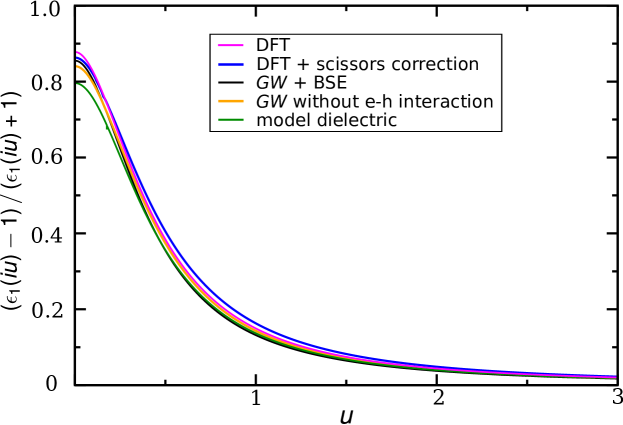
Figure 1: $\left(\epsilon_{1}\left(iu\right)-1\right)/\left(\epsilon_{1}\left(iu\right)+1\right)$ of silicon with respect to frequency $u$ (in hartree) calculated from DFT, DFT+scissors correction, $GW$, $GW$+BSE and model dielectric function.

GaAs

Fig. 2 shows the computed dielectric functions of GaAs. $GW$ and $GW$+BSE show very similar dielectric functions, indicating the weak exciton effect in GaAsNam et al. (1976), and strong dielectric screening effect. DFT and model dielectric functions slightly underestimate $GW$+BSE values, which is because of the higher absorption calculated with $GW$ and $GW$+BSE than that with DFT. In general, similar to silicon, all the methods yield dielectric functions close to each other, in particular in the high-frequency region. This similarity is largely due to the fact that both semiconductors have similar band gaps and dielectric constants, as shown in Table 1.

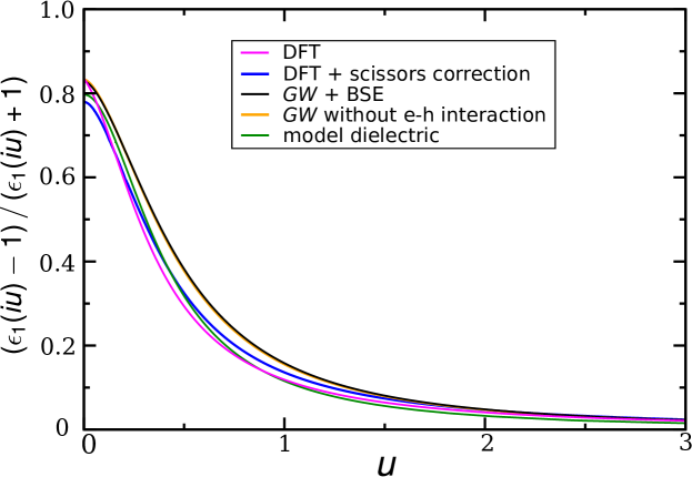
Figure 2: $\left(\epsilon_{1}\left(iu\right)-1\right)/\left(\epsilon_{1}\left(iu\right)+1\right)$ of GaAs with respect to frequency $u$ (in hartree) calculated from DFT, DFT+scissors correction, $GW$, $GW$+BSE, and model dielectric function.

Diamond

The dielectric function of diamond is shown in Fig. 3. Diamond shares similar geometric and electronic structures with silicon, but with much larger band gap. In this case, the overestimation of dielectric function from DFT and the underestimation from model dielectric function are more pronounced than those for silicon at low frequencies. This difference is mainly due to the discrepancy between the Penn model effective band gap (slightly overestimated) and the $GW$ or $GW$+BSE value. However, as energy increases to the high-energy region, this discrepancy vanishes, matching the model dielectric function to $GW$+BSE results very well.

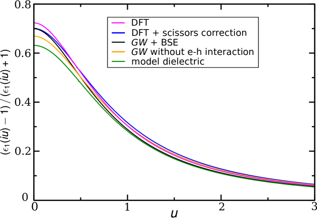
Figure 3: $\left(\epsilon_{1}\left(iu\right)-1\right)/\left(\epsilon_{1}\left(iu\right)+1\right)$ of diamond with respect to frequency $u$ (in hartree) calculated from DFT, DFT+scissors correction, $GW$, $GW$+BSE, and model dielectric function.

LiF

LiF is a prototypical material with strong exciton effect on its optical absorption Abbamonte et al. (2008). As shown in Fig. 4, at low energies, $GW$+BSE including electron-hole interaction yields higher value compared to the dielectric function without electron-hole interaction, which corresponds to the exciton absorption. Due to the same discrepancy observed in diamond, the model dielectric function underestimates the response near zero energy, but matches $GW$-BSE result well in the high-energy region. The vdW coefficients measure the strength of the dielectric response of a bulk solid to the instantaneously induced multipole moment of the adsorbed atom or molecule. They are integrated over the whole energy range, including both low-energy and high-energy dielectric contributions. Thus, the noticeable discrepancy observed in the low-energy part has minor effect on the overall vdW coefficients. However, the DFT-calculated dielectric response seriously overestimates the response in the whole energy spectrum, compared to $GW$+BSE, leading to significantly overestimated vdW coefficients, as shown in the Table LABEL:si_vdw. This overestimation problem cannot be fixed even with scissors correction to the DFT band gap. Comparison of $GW$-BSE with $GW$ (without electron-hole interaction) suggests that there is an important exciton effect on the dielectric function in the low-energy range. This suggests that semilocal DFT may not fully capture this exciton effect as well as the many-body effect. As a result, semilocal DFT tends to overestimate the dielectric function, although it slightly underestimates the dielectric function for semiconductors.

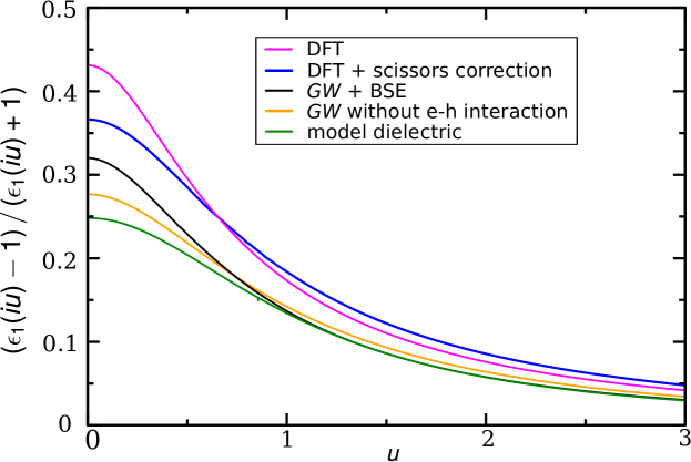
Figure 4: $\left(\epsilon_{1}\left(iu\right)-1\right)/\left(\epsilon_{1}\left(iu\right)+1\right)$ of LiF with respect to frequency $u$ (in hartree) calculated from DFT, DFT+scissors correction, $GW$, $GW$+BSE, and model dielectric function.

NaF

NaF is another prototypical material with strong exciton effects. Figure 4 shows the comparison of the dielectric function evaluated with all the methods discussed above. From Fig 4, we observe that the model dielectric function still underestimates the response near zero frequency, but with overall good quality matching of $GW$+BSE results. However, semilocal DFT and scissors-corrected semilocal DFT strongly overestimate the dielectric function magnitude for the whole frequency range, reflecting the inadequacy of semilocal DFT, as observed in other ionic solids.

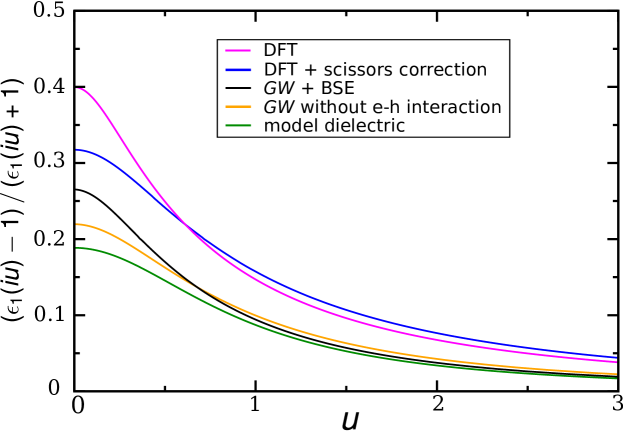
Figure 5: $\left(\epsilon_{1}\left(iu\right)-1\right)/\left(\epsilon_{1}\left(iu\right)+1\right)$ of NaF with respect to frequency $u$ (in hartree) calculated from DFT, DFT+scissors correction, $GW$, $GW$+BSE, and model dielectric function.

MgO

As a support for variety of catalytic reactions Zhang et al. (2007); Yoon et al. (2005), MgO has attracted great attension in recent years. Accurate calculation of the dielectric function for the vdW interaction is significantly important for the prediction of the correct chemical reaction path and energy barrier. As shown in Fig. 6, MgO also shows strong exciton effect, leading to obvious but less pronounced deviation of the DFT curve from the $GW$+BSE calculation, compared to other ionic solids considered here. On the other hand, the model dielectric function agrees with $GW$+BSE values rather well.

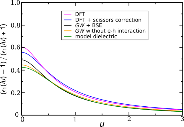
Figure 6: $\left(\epsilon_{1}\left(iu\right)-1\right)/\left(\epsilon_{1}\left(iu\right)+1\right)$ of MgO with respect to frequency $u$ (in hartree) calculated from DFT, DFT+scissors correction, $GW$, $GW$+BSE, and model dielectric function.

III.2 vdW Coefficients for adsorption on surfaces of solids

The vdW coefficients $C_{3}$ and $C_{5}$ can be calculated from Eq. (8) with the model dynamic multipole polarizability given by Tao et al. (2012)

$$\alpha_{l}(iu)=\frac{2l+1}{4\pi d_{l}}\int_{0}^{R_{l}}dr~{}4\pi r^{2}\frac{r^{2l-2}~{}d_{l}^{4}\omega_{l}^{2}}{d_{l}^{4}\omega_{l}^{2}+u^{2}},$$ (9)

where $R_{l}$ is the effective vdW radius and $d_{l}$ is a parameter introduced to satisfy the exact zero- and high-frequency limits. Numerical tests show that the model can generate vdW coefficients for diverse atom pairs in excellent agreement with accurate reference values, with mean absolute relative error of only $3\%$. To benchmark our model dielectric function for adsorption, we calculate the vdW coefficients with several dielectric functions obtained from $GW$, $GW$+BSE and DFT-GGA methods, and compare them to the vdW coefficients obtained from the model dielectric function and accurate reference values. The results are shown in Table LABEL:si_vdw.

From Table LABEL:si_vdw, we observe that the vdW coefficients calculated from the model dielectric function are close to the reference values. They agree quite well with the $GW$ and $GW$+BSE values, with mean absolute relative deviations of 2% for $C_{3}$ and 5% $C_{5}$ from those calculated with the $GW$ dielectric function, and 4% for $C_{3}$ and 8% for $C_{5}$ from those evaluated with the $GW$+BSE dielectric function, respectively. The strong exciton observed in ionic solids LiF, NaF and MgO has some effect on the vdW coefficients. But this effect is relatively small for the vdW coefficients evaluated with $GW$ and $GW$+BSE dielectric function, as the dielectric enhancement by exitons only appears within small frequency range. The model dielectric function can also accounts for exitons via the static dielectric function part, the vdW coefficients evaluated from the model dielectric function agree reasonably well with these two ab initio values even for materials with strong exiton effect, as found in the ionic solids considered here. However, we find that the DFT-GGA significantly overestimates vdW coefficients by 30% for $C_{3}$ and 33% for $C_{5}$, due to the overestimation of the dielectric functions in the whole frequency range. Moreover, scissors correction to the DFT dielectric function shows little improvement of vdW coefficient. The detail of DFT calculations can be found from Table LABEL:si_vdw.

Table 2: vdW coefficients (in a.u.) between rare gas atoms and the surfaces of semiconductors and insulators. These are calculated by DFT, DFT+ scissors, $GW$, $GW$+BSE, and model dielectric. The reference values of He atom on all surfaces are from Ref. 24. Values for other atoms are from Ref. 74. MRE = mean relative error. MARE = mean absolute relative error.

	DFT		DFT+sci.		$GW$		$GW$+BSE		Model diele.		Reference
Silicon	$C_{3}$	$C_{5}$	$C_{3}$	$C_{5}$	$C_{3}$	$C_{5}$	$C_{3}$	$C_{5}$	$C_{3}$	$C_{5}$	$C_{3}$	$C_{5}$
H	0.105	0.416	0.107	0.425	0.100	0.395	0.101	0.402	0.096	0.383	0.102	0.366
He	0.046	0.083	0.047	0.086	0.043	0.078	0.044	0.080	0.042	0.076	0.042	0.076
Ne	0.096	0.262	0.099	0.270	0.090	0.246	0.093	0.253	0.088	0.241	0.089	0.241
Ar	0.330	1.632	0.338	1.676	0.312	1.541	0.319	1.578	0.304	1.502	0.310	1.490
Kr	0.468	2.888	0.479	2.959	0.443	2.735	0.452	2.794	0.431	2.659	0.449	2.644
Xe	0.802	6.613	0.822	6.782	0.758	6.254	0.775	6.395	0.738	6.088	0.655	5.469
GaAs	$C_{3}$	$C_{5}$	$C_{3}$	$C_{5}$	$C_{3}$	$C_{5}$	$C_{3}$	$C_{5}$	$C_{3}$	$C_{5}$	$C_{3}$	$C_{5}$
H	0.089	0.350	0.091	0.361	0.100	0.400	0.101	0.401	0.092	0.362	0.091	0.351
He	0.038	0.069	0.040	0.073	0.044	0.081	0.045	0.081	0.039	0.071	0.041	0.072
Ne	0.080	0.219	0.084	0.230	0.093	0.255	0.094	0.256	0.082	0.224	0.081	0.227
Ar	0.277	1.364	0.287	1.422	0.318	1.577	0.320	1.585	0.285	1.407	0.285	1.417
Kr	0.393	2.420	0.407	2.513	0.451	2.785	0.453	2.797	0.406	2.500	0.412	2.523
Xe	0.674	5.548	0.701	5.768	0.775	6.386	0.779	6.416	0.693	5.715	0.603	5.242
Diamond	$C_{3}$	$C_{5}$	$C_{3}$	$C_{5}$	$C_{3}$	$C_{5}$	$C_{3}$	$C_{5}$	$C_{3}$	$C_{5}$	$C_{3}$	$C_{5}$
H	0.113	0.470	0.112	0.468	0.108	0.448	0.109	0.452	0.101	0.422	0.112	0.407
He	0.057	0.105	0.057	0.106	0.054	0.102	0.054	0.101	0.051	0.095	0.051	0.097
Ne	0.123	0.334	0.124	0.338	0.119	0.323	0.118	0.320	0.110	0.300	0.116	0.308
Ar	0.390	1.961	0.061	0.257	0.374	1.882	0.374	1.881	0.350	1.761	0.375	1.781
Kr	0.543	3.378	0.542	3.378	0.519	3.233	0.521	3.243	0.486	3.032	0.526	3.069
Xe	0.960	7.857	0.963	7.871	0.922	7.534	0.921	7.539	0.861	7.047	0.737	6.132
LiF	$C_{3}$	$C_{5}$	$C_{3}$	$C_{5}$	$C_{3}$	$C_{5}$	$C_{3}$	$C_{5}$	$C_{3}$	$C_{5}$	$C_{3}$	$C_{5}$
H	0.066	0.276	0.061	0.257	0.046	0.194	0.050	0.208	0.042	0.178	0.048	0.169
He	0.033	0.062	0.032	0.060	0.024	0.045	0.025	0.047	0.022	0.041	0.023	0.042
Ne	0.073	0.198	0.071	0.192	0.052	0.142	0.055	0.148	0.048	0.131	0.048	0.133
Ar	0.229	1.153	0.218	1.097	0.163	0.821	0.173	0.868	0.150	0.756	0.155	0.756
Kr	0.320	1.984	0.302	1.872	0.225	1.405	0.240	1.494	0.207	1.292	0.219	1.294
Xe	0.568	4.631	0.541	4.395	0.402	3.281	0.425	3.475	0.370	3.019	0.313	2.561
NaF	$C_{3}$	$C_{5}$	$C_{3}$	$C_{5}$	$C_{3}$	$C_{5}$	$C_{3}$	$C_{5}$	$C_{3}$	$C_{5}$	$C_{3}$	$C_{5}$
H	0.059	0.241	0.052	0.220	0.035	0.146	0.039	0.160	0.035	0.147	0.038	0.137
He	0.029	0.054	0.027	0.052	0.018	0.033	0.019	0.035	0.018	0.033	0.018	0.033
Ne	0.064	0.172	0.061	0.165	0.039	0.105	0.041	0.111	0.039	0.105	0.037	0.104
Ar	0.200	1.005	0.186	0.940	0.122	0.613	0.131	0.657	0.122	0.615	0.123	0.600
Kr	0.280	1.733	0.258	1.603	0.169	1.054	0.183	1.138	0.170	1.058	0.174	1.032
Xe	0.495	4.040	0.463	3.764	0.300	2.454	0.322	2.638	0.301	2.462	0.248	2.059
MgO	$C_{3}$	$C_{5}$	$C_{3}$	$C_{5}$	$C_{3}$	$C_{5}$	$C_{3}$	$C_{5}$	$C_{3}$	$C_{5}$	$C_{3}$	$C_{5}$
H	0.087	0.358	0.085	0.352	0.069	0.286	0.072	0.295	0.063	0.259	0.069	0.252
He	0.042	0.079	0.042	0.079	0.034	0.064	0.035	0.064	0.031	0.057	0.032	0.059
Ne	0.092	0.249	0.092	0.250	0.074	0.202	0.075	0.204	0.067	0.182	0.066	0.188
Ar	0.295	1.476	0.292	1.465	0.237	1.189	0.242	1.212	0.214	1.073	0.224	1.094
Kr	0.412	2.557	0.407	2.527	0.329	2.050	0.338	2.101	0.298	1.854	0.315	1.892
Xe	0.725	5.934	0.719	5.880	0.582	4.764	0.594	4.867	0.524	4.299	0.439	3.796
MRE(%)	29.3	32.4	27.0	30.4	7.2	9.7	10.2	12.9	1.3	3.7	-	-
MARE(%)	30.3	33.2	27.3	30.4	8.5	9.7	10.5	12.9	6.7	4.6	-	-

IV Conclusion

In summary, we have calculated the frequency-dependent dielectric function of semiconductors and insulators with the DFT-GGA, $GW$ and $GW$+BSE methods. Based on these calculations, we study the accuracy of the modified Penn model by comparing the model dielectric function to the highly-accurate $GW$ and $GW$+BSE methods. We find that the model dielectric function agrees quite well with these two methods, in particular for small energy-gap semiconductors. However, a noticeable discrepancy arises with the increase of band gap. A similar trend has been also observed with the DFT-GGA dielectric function, which shows even greater disagreement with the $GW$ and $GW$+BSE methods, compared to the model dielectric function. To have a better understanding of the DFT-GGA method, we adjust the GGA band gap up to the experimental value (scissors correction). We find that this adjustment does improve the agreement of DFT-GGA with the benchmark methods, but the improvement is not nearly enough. Then we calculate the vdW coefficients $C_{3}$ and $C_{5}$ for atoms on the surface of semiconductors and insulators with the model dynamic multipole polarizability and the dielectric functions obtained from the modified Penn model, DFT-GGA, $GW$, and $GW$+BSE methods. The results show that, except for the vdW coefficients obtained with the DFT-GGA dielectric function, they all agree well with each other. The deviations of the vdW coefficients obtained with the model dielectric function from those obtained with the $GW$+BSE dielectric function are 4% for $C_{3}$ and 8% for $C_{5}$, respectively. The deviation is even smaller between the vdW coefficients obtained from the model dielectric function and the $GW$ method. However, these deviations become significantly larger for the DFT-GGA ($C_{3}$: 29%, $C_{5}$: 29%) or scissor-corrected ($C_{3}$: 24%, $C_{5}$: 24%) dielectric function, suggesting the significance of electronic nonlocality that is missing in semilocal DFT, leading to the bad performance for the dielectric function of ionic solids with strong exciton effect.

V Acknowledgment

FZ acknowledges support from NSF under Grant no. DMR-1124696. JT acknowledges support from NSF under Grant no. CHE-1261918 and the Office of Naval Research under grant No. N00014-14-1-0761. AMR was supported by the Department of Energy Office of Basic Energy Sciences, under Grant no. DE-FG02-07ER15920. Computational support was provided by the HPCMO and the NERSC.

References

- Marques et al. (2011) M. A. L. Marques, J. Vidal, M. J. T. Oliveira, L. Reining, and S. Botti, Phys. Rev. B 83, 035119 (2011).
- Skone et al. (2014) J. H. Skone, M. Govoni, and G. Galli, Phys. Rev. B 89, 195112 (2014).
- Geim and Grigorieva (2013) A. K. Geim and I. V. Grigorieva, Nature 499, 419 (2013).
- Perdew et al. (1996) J. P. Perdew, K. Burke, and M. Ernzerhof, Phys. Rev. Lett. 77, 3865 (1996).
- Tao et al. (2003) J. Tao, J. P. Perdew, V. N. Staroverov, and G. E. Scuseria, Phys. Rev. Lett. 91, 146401 (2003).
- Perdew and Levy (1983) J. P. Perdew and M. Levy, Phys. Rev. Lett. 51, 1884 (1983).
- Sham and Schlüter (1983) L. J. Sham and M. Schlüter, Phys. Rev. Lett. 51, 1888 (1983).
- Janak (1978) J. Janak, Phys. Rev. B 18, 7165 (1978).
- Perdew et al. (1982) J. P. Perdew, R. G. Parr, M. Levy, and J. L. Balduz Jr, Phys. Rev. Lett. 49, 1691 (1982).
- Hedin (1965) L. Hedin, Phys. Rev. 139, A796 (1965).
- Zhu and Louie (1991) X. Zhu and S. G. Louie, Phys. Rev. B 43, 14142 (1991).
- Onida et al. (2002) G. Onida, L. Reining, and A. Rubio, Rev. Mod. Phys. 74, 601 (2002).
- Onida et al. (1995) G. Onida, L. Reining, R. Godby, R. Del Sole, and W. Andreoni, Phys. Rev. lett. 75, 818 (1995).
- Rohlfing and Louie (1998) M. Rohlfing and S. G. Louie, Phys. Rev. lett. 81, 2312 (1998).
- Schleife et al. (2009) A. Schleife, C. Rödl, F. Fuchs, J. Furthmüller, and F. Bechstedt, Phys. Rev. B 80, 035112 (2009).
- Hsueh et al. (2011) H. Hsueh, G. Guo, and S. G. Louie, Phys. Rev. B 84, 085404 (2011).
- Qiu et al. (2013) D. Y. Qiu, H. Felipe, and S. G. Louie, Phys. Rev. lett. 111, 216805 (2013).
- Penn (1962) D. R. Penn, Phys. Rev. 128, 2093 (1962).
- Penn (1987) D. R. Penn, Phys. Rev. B 35, 482 (1987).
- Levine and Louie (1982) Z. H. Levine and S. G. Louie, Phys. Rev. B 25, 6310 (1982).
- Lines (1990) M. Lines, Phys. Rev. B 41, 3372 (1990).
- Kim et al. (1992) C. C. Kim, J. W. Garland, H. Abad, and P. M. Raccah, Phys. Rev. B 45, 11749 (1992).
- Breckenridge et al. (1974) R. A. Breckenridge, R. W. Shaw Jr, and A. Sher, Phys. Rev. B 10, 2483 (1974).
- Vidali and Cole (1981a) G. Vidali and M. Cole, Surface Science Letters 107, L374 (1981a).
- Tao et al. (2015) J. Tao, J. Yang, and A. M. Rappe, The Journal of Chemical Physics 142, 164302 (2015).
- Tao and Rappe (2014) J. Tao and A. M. Rappe, Phys. Rev. Lett. 112, 106101 (2014).
- Levine and Allan (1989) Z. H. Levine and D. C. Allan, Phys. Rev. Lett. 63, 1719 (1989).
- Van Vechten (1969) J. A. Van Vechten, Phys. Rev. 182, 891 (1969).
- Philipp and Ehrenreich (1962) H. R. Philipp and H. Ehrenreich, Phys. Rev. Lett. 8, 92 (1962).
- Philipp and Ehrenreich (1963) H. R. Philipp and H. Ehrenreich, Phys. Rev. 129, 1550 (1963).
- Sturge (1962) M. D. Sturge, Phys. Rev. 127, 768 (1962).
- Willardsen and Beer (1981) R. Willardsen and A. Beer, Semiconductors and Semimetals, Vol. 3 (Academic Press, 1981).
- Giannozzi et al. (2009) P. Giannozzi, S. Baroni, N. Bonini, M. Calandra, R. Car, C. Cavazzoni, D. Ceresoli, G. L. Chiarotti, M. Cococcioni, I. Dabo, A. D. Corso, S. de Gironcoli, S. Fabris, G. Fratesi, R. Gebauer, U. Gerstmann, C. Gougoussis, A. Kokalj, M. Lazzeri, L. Martin-Samos, N. Marzari, F. Mauri, R. Mazzarello, S. Paolini, A. Pasquarello, L. Paulatto, C. Sbraccia, S. Scandolo, G. Sclauzero, A. P. Seitsonen, A. Smogunov, P. Umari, and R. M. Wentzcovitch, J. Phys.: Condens. Matter 21, 395502 (2009).
- Rappe et al. (1990) A. M. Rappe, K. M. Rabe, E. Kaxiras, and J. D. Joannopoulos, Phys. Rev. B Rapid Comm. 41, 1227 (1990).
- Ramer and Rappe (1999) N. J. Ramer and A. M. Rappe, Phys. Rev. B 59, 12471 (1999).
- Nastos et al. (2005) F. Nastos, B. Olejnik, K. Schwarz, and J. E. Sipe, Phys Rev B 72, 045223 (2005).
- Hybertsen and Louie (1986) M. S. Hybertsen and S. G. Louie, Phys. Rev. B 34, 5390 (1986).
- Rohlfing and Louie (2000) M. Rohlfing and S. G. Louie, Phys. Rev. B 62, 4927 (2000).
- Deslippe et al. (2012) J. Deslippe, G. Samsonidze, D. A. Strubbe, M. Jain, M. L. Cohen, and S. G. Louie, Computer Physics Communications 183, 1269 (2012).
- Malone and Cohen (2013) B. D. Malone and M. L. Cohen, Journal of Physics: Condensed Matter 25, 105503 (2013).
- Dion et al. (2004) M. Dion, H. Rydberg, E. Schröder, D. C. Langreth, and B. I. Lundqvist, Phys. Rev. Lett. 92, 246401 (2004).
- Granatier et al. (2011) J. Granatier, P. Lazar, M. Otyepka, and P. Hobza, J. Chem. Theory. Comput. 7, 3743 (2011).
- Klimeš et al. (2011) J. Klimeš, D. R. Bowler, and A. Michaelides, Phys. Rev. B 83, 195131 (2011).
- Lazić et al. (2005) P. Lazić, Ž. Crljen, R. Brako, and B. Gumhalter, Phys. Rev. B 72, 245407 (2005).
- Chen et al. (2012) D.-L. Chen, W. Al-Saidi, and J. K. Johnson, Journal of Physics: Condensed Matter 24, 424211 (2012).
- Grimme (2004) S. Grimme, J. Comput. Chem. 25, 1463 (2004).
- Becke and Johnson (2007) A. D. Becke and E. R. Johnson, J. Chem. Phys. 127, 154108 (2007).
- Tkatchenko and Scheffler (2009) A. Tkatchenko and M. Scheffler, Phys. Rev. lett. 102, 073005 (2009).
- Silvestrelli (2008) P. L. Silvestrelli, Phys. Rev. lett. 100, 053002 (2008).
- Tkatchenko et al. (2013) A. Tkatchenko, A. Ambrosetti, and R. A. DiStasio Jr, J. Chem. Phys. 138, 074106 (2013).
- Tao et al. (2010) J. Tao, J. P. Perdew, and A. Ruzsinszky, Phys. Rev. B 81, 233102 (2010).
- Tao et al. (2012) J. Tao, J. P. Perdew, and A. Ruzsinszky, Proc. Natl. Acad. Sci. 109, 18 (2012).
- Tao and Perdew (2014) J. Tao and J. P. Perdew, The Journal of Chemical Physics 141, 141101 (2014).
- Tao and Rappe (2016) J. Tao and A. M. Rappe, The Journal of Chemical Physics 144, 031102 (2016).
- Grimme et al. (2010) S. Grimme, J. Antony, S. Ehrlich, and H. Krieg, J. Chem. Phys. 132, 154104 (2010).
- Grimme (2006) S. Grimme, J. Comput. Chem. 27, 1787 (2006).
- Ruiz et al. (2012) V. G. Ruiz, W. Liu, E. Zojer, M. Scheffler, and A. Tkatchenko, Phys. Rev. lett. 108, 146103 (2012).
- Ma et al. (2011) J. Ma, A. Michaelides, D. Alfè, L. Schimka, G. Kresse, and E. Wang, Phys. Rev. B 84, 033402 (2011).
- Fang et al. (2012) H. Fang, P. Kamakoti, J. Zang, S. Cundy, C. Paur, P. I. Ravikovitch, and D. S. Sholl, J. Phys. Chem. C 116, 10692 (2012).
- Sirtl et al. (2013) T. Sirtl, J. Jelic, J. Meyer, K. Das, W. M. Heckl, W. Moritz, J. Rundgren, M. Schmittel, K. Reuter, and M. Lackinger, Phys. Chem. Chem. Phys. 15, 11054 (2013).
- Schmidt et al. (1993) M. W. Schmidt, K. K. Baldridge, J. A. Boatz, S. T. Elbert, M. S. Gordon, J. H. Jensen, S. Koseki, N. Matsunaga, K. A. Nguyen, S. J. Su, T. L. Windus, M. Dupuis, and J. A. Montgomery, J. Comput. Chem. 14, 1347 (1993).
- Dykstra et al. (2011) C. Dykstra, G. Frenking, K. Kim, and G. Scuseria, Theory and applications of computational chemistry: the first forty years (Elsevier, 2011).
- Dalvit et al. (2011) D. Dalvit, P. Milonni, D. Roberts, and F. d. Rosa, Casimir Physics - (Springer, Berlin, Heidelberg, 2011).
- Zaremba and Kohn (1976) E. Zaremba and W. Kohn, Phys. Rev. B 13, 2270 (1976).
- hui Yang et al. (2015) Z. hui Yang, F. Sottile, and C. A. Ullrich, Phys. Rev. B 92, 035202 (2015).
- Aulbur et al. (1999) W. G. Aulbur, L. Jönsson, and J. W. Wilkins, in Solid State Physics (Elsevier BV, 1999) pp. 1–218.
- van Faassen et al. (2002) M. van Faassen, P. L. de Boeij, R. van Leeuwen, J. A. Berger, and J. G. Snijders, Phys. Rev. Lett. 88, 186401 (2002).
- van Faassen et al. (2003) M. van Faassen, P. L. de Boeij, R. van Leeuwen, J. A. Berger, and J. G. Snijders, The Journal of Chemical Physics 118, 1044 (2003).
- Poole et al. (1975) R. Poole, J. Jenkin, J. Liesegang, and R. Leckey, Phys. Rev. B 11, 5179 (1975).
- Nam et al. (1976) S. B. Nam, D. C. Reynolds, C. W. Litton, R. J. Almassy, T. C. Collins, and C. M. Wolfe, Phys. Rev. B 13, 761 (1976).
- Abbamonte et al. (2008) P. Abbamonte, T. Graber, J. P. Reed, S. Smadici, C.-L. Yeh, A. Shukla, J.-P. Rueff, and W. Ku, Proc. Natl. Acad. Sci. 105, 12159 (2008).
- Zhang et al. (2007) C. Zhang, B. Yoon, and U. Landman, J. Am. Chem. Soc. 129, 2228 (2007).
- Yoon et al. (2005) B. Yoon, H. Hakkinen, U. Landman, A. S. Worz, J. M. Antonietti, S. Abbet, K. Judai, and U. Heiz, Science 307, 403 (2005).
- Vidali and Cole (1981b) G. Vidali and M. Cole, Surface Science 110, 10 (1981b).