The dynamics of a spinning particle in a linear in spin Hamiltonian approximation

Abstract

We investigate for order and chaos the dynamical system of a spinning test particle of mass $m$ moving in the spacetime background of a Kerr black hole of mass $M$. This system is approximated in our investigation by the linear in spin Hamiltonian function provided in [E. Barausse, and A. Buonanno, Phys.Rev. D 81, 084024 (2010)]. We study the corresponding phase space by using 2D projections on a surface of section and the method of color and rotation on a 4D Poincaré section. Various topological structures coming from the non-integrability of the linear in spin Hamiltonian are found and discussed. Moreover, an interesting result is that from the value of the dimensionless spin $S/(m~{}M)=10^{-4}$ of the particle and below, the impact of the non-integrability of the system on the motion of the particle seems to be negligible.

I Introduction

Mathisson Mathisson37 and Papapetrou Papapetrou51 provided the equations of motion for a spinning particle in a curved spacetime. The equations of motion of a spinning test particle are interesting from the astrophysical point of view, because they approximate the motion of a stellar compact object in the spacetime background of a supermassive black hole. Such a binary system is called an extreme mass ratio inspiral (EMRI). EMRIs are among the most promising sources of gravitational waves expected to be detected by space interferometer antennas like LISA (see, e.g., LISA ). However, in this work we focus rather on the dynamics of a spinning particle system than on astrophysical aspects.

The number of Mathisson-Papapetrou (MP) equations is smaller than the number of variables which the MP equations intend to evolve. The above fact can be interpreted as a freedom of choosing different worldlines for evolving the equation of motion of the same extended object described by the pole-dipole approximation Moeller49 . To choose a worldline we use a supplementary condition that is known in the literature as the spin supplementary condition (SSC). There is a variety of SSCs (for a review, see, e.g., Semerak99 ; Kyrian07 ; Semerak15 ), but all are physically acceptable. The most renown are the Pirani (P) Pirani56 and the Tulczyjew (T) Tulczyjew59 SSCs. For many years the P SSC was considered unphysical, because the test particle exhibited helical motion in the flat spacetime limit. However, in Costa12 it has been shown that this helical motion results from a hidden momentum and the P SSC is physically valid as well.

The aspect of the spinning particle dynamics we are interested in is the issue of the integrability of the corresponding system. It has been shown that for the Schwarzschild background the MP equations with T SSC give chaotic orbits Suzuki97 , and the same holds for the Kerr background, see, e.g., Hartl03a ; Hartl03b ; Han08 . Hence, one can claim that the MP equations with T SSC correspond to a non-integrable system. However, in the linear in spin approximation of the MP equations, it has been proved that for the T SSC a Killing-Yano tensor provides a Carter-like constant of motion for the Kerr background Rudiger . The existence of a Carter-like constant and the fact that the T and P SSCs are the same in the linear regime led to the impression that in the linear in spin approximation the spinning particle dynamics corresponds to an integrable system (see, e.g., Hinderer13 ). For geodesic orbits in a Kerr spacetime the existence of the Carter constant ensures integrability, since it is the fourth constant of motion (the others being the energy, the angular momentum along the symmetry axis and the contraction of the four-momentum) in a Hamiltonian system of four degrees of freedom. Nevertheless, when the particle is spinning we have extra degrees of freedom, and it is questionable even if the existence of a Carter-like constant can ensure the integrability of the system.

When examining whether a system is integrable or not, it is useful to have a canonical Hamiltonian formalism which provides symplecticity. In a non-symplectic system we need as many constants of motion as the dimensionality of the phase space. On the other hand, in a canonical Hamiltonian system two dimensions of the phase space correspond to one degree of freedom. Therefore, we need half the number of constants of motion in order to have integrability with respect to a non-canonical system of the same phase space dimensionality. Moreover, by having a canonical Hamiltonian system, tools like Poincaré sections can be properly used. When a system is not symplectic, then a surface of section is ambiguous. A canonical Hamiltonian formalism has not been found yet for the MP equations with the T SSC. However, such canonical Hamiltonian formalism has been provided in Barausse09 for the Newton-Wigner (NW) SSC NewtonWigner49 in the linearized in spin approximation.

A Hamiltonian for a spinning particle moving in a Kerr spacetime background has been first provided in Barausse09 . However, due to the approximative procedure which leads from the MP equations to the linearized in spin Hamiltonian function, the resulting Hamiltonian equations are not equivalent to the corresponding MP equations, e.g., starting the Hamiltonian equations and the MP equations with the same initial conditions lead to two diferrent orbits LGSK . It might even occur that the final linearized Hamiltonian system may not even respect some symmetries that the corresponding MP equations respect. For example, the Hamiltonian function provided in Barausse09 for the Kerr spacetime in Boyer-Lindquist coordinates did not respect in the Schwarzschild limit $a=0$ the spherical background symmetry. Namely, the total angular momentum was not preserved as it should be. Absence of integrals of motions could lead to the misleading impression that for the Schwarzschild background the Hamiltonian corresponds to a non-integrable system (see, e.g., figure 2 in KLLS ). The problem with the Hamiltonian in Barausse09 was the specific tetrad field choice on which the Hamiltonian function was built on. Even in Barausse09 , it was found that the resulting Hamiltonian would evolve the spin in the flat spacetime limit Barausse09 . However, since the helical motion in the case of the MP equations with P SSC could result from a hidden momentum, the same could hold for the Hamiltonian approximation coming from the NW SSC. Thus, a more solid reasoning was needed to show the drawbacks of the tetrad field chosen in Barausse09 . In KLLS it was shown that if the resulting Hamiltonian should respect the symmetries of the Schwarzschild background, then the corresponding tetrad filed should obey a certain prescription (equation (44) in KLLS ). The tetrad field of Barausse09 is not complying with this prescription.

On the other hand, a different tetrad field choise provided in Barausse10 led to a revised Hamiltonian for the Kerr background. This tetrad field is obeying the prescription given in KLLS . In particular, for the Schwarzschild limit the revised Hamiltonian Barausse10 was conserving not only the total angular momentum as it should be, but it was shown in KLLS that the magnitude of the orbital momentum was preserved as well. The latter implies that in the Schwarzschild limit the revised Hamiltonian of Barausse10 corresponds to an integrable system, since for a five degrees of freedom system we have five constants of motion KLLS . The revised Hamiltonian ceases to be integrable when the spin of the central black hole is nonzero KLLS , i.e., in the Kerr spacetime background. A thorough study of the non-integrability of the revised Hamiltonian is the subject of our article.

The study of chaotic motion around black holes probably starts with Contopoulos90 , where a method based on Cantor sets was applied to prove the chaotic nature of the system. Since then many methods have been applied to detect chaos in the vicinity of black holes, but the most common is the 2D Poincaré section. It is a fact that in order to study the non-integrability of a two degrees of freedom Hamiltonian system a 2D Poincaré section is a standard tool. However, since the Hamiltonian provided in Barausse10 corresponds to a system with three degrees of freedom, we have to deal with 4D Poincaré sections Contopoulos02 . In order to detect order and chaos in the 4D Poincaré spaces of section, we must first of all have a way to visualize them. In the past, several methods have been proposed for the visualization of the 4D surfaces of section in a 6D phase space of a 3D autonomus Hamiltonian system: ordinary 2D projections Contopoulos89 , 3D projections Vrahatis97 , stereoscopic projections Froeschle70 ; Martinet81 ; Contopoulos82 , or 2D slices of 3D subspaces (Froeschle70 ; Froeschle72 , and recently a more sophisticated version in Richter14 ; Lange14 (see Appendix).

In the present work we use the method of color and rotation, introduced by Patsis and Zachilas Patsis94 . This method is extensively described for the case of 3D rotating galactic potentials in a series of papers Katsanikas11a ; Katsanikas11b ; Katsanikas11c ; Katsanikas13 ; Patsis14a ; Patsis14b . These papers investigate portraits of the 4D spaces of section in the neighborhood of periodic orbits exhibiting all kinds of instabilities encountered in 3D Hamiltonian systems (see, e.g., Contopoulos02 ). The method has also been applied in the study of the structure of the phase space close to fixed points in a 4D symplectic map Zachilas13 , and to design spacecraft orbits Geisel13 .

The method consists in plotting the points (the consequents) of an orbit in a 3D subspace as they cross the space of section in a given direction, rotate them by means of standard 3D graphic tools to get a good insight of their distribution in the 3D subspace, and finally color them according to their value in the fourth dimension (the one not used in the 3D spatial representation of the orbit). Color allows the estimation of the smoothness in the 4th dimension of geometrical structures appearing in the 3D projections and the distinction of pseudo- from true intersections in the 4D space. Thus, one can establish criteria for the regular, weak chaotic or strong chaotic character of a given orbit Patsis94 ; Katsanikas11a ; Katsanikas11b ; Katsanikas11c ; Katsanikas13 ; Patsis14a ; Patsis14b ; Zachilas13 . In the latter papers, specific patterns in phase space are associated with the various kinds of instability or with stability. In our paper this method is used in the study of the dynamics of a spinning particle in the Hamiltonian approach in an effort to trace regular and chaotic motion in the phase space of our system.

The paper is organized as follows. Sec. II introduces the Hamiltonian function of Barausse10 , which we use for our study. Sec. III discusses the non-integrability of the Hamiltonian, briefly describes the setting up of the numerics, and provides a detailed account of our numerical findings. Sec. IV sums up our findings, and discusses the possible astrophysical implications. Appendix A lists techniques used for visualizing 4D spaces of section.

We use geometric units, i.e., $G=c=1$, and the signature of the metric is (-,+,+,+). Greek letters denote the indices corresponding to spacetime (running from 0 to 3), while Latin letters denote indices corresponding only to space (running from 1 to 3).

II The Hamiltonian of a spinning particle

The canonical Hamiltonian formalism of a spinning particle in Barausse09 has been achieved by linearizing the MP equations of motion for the NW SSC. In this formalism the mass of the test particle $m$ is considered a constant of motion Barausse09 , and the spin of the particle is given by a three vector $S^{I}$. The corresponding Hamiltonian function $H$ splits in two main parts, the non-spinning $H_{NS}$, which describes basically the geodesic motion, and the spinning part $H_{S}$, which incorporates the spinning of the particle, i.e.,

$$H=H_{NS}+H_{S}~{}~{}.$$ (1)

The non-spinning part of the Hamiltonian $H_{NS}$ reads

$$H_{NS}=\beta^{i}P_{i}+\alpha~{}\sqrt{m^{2}+\gamma^{ij}P_{i}P_{j}}~{}~{},$$ (2)

where $P_{i}$ are the canonical momenta conjugate to the coordinates $x^{i}$ of the Hamiltonian (1) Barausse09 , and

$$\alpha = \frac{1}{\sqrt{-g^{00}}}~{}~{},$$

$$\beta^{i} = \frac{g^{0i}}{g^{00}}~{}~{},$$

$$\gamma^{ij} = g^{ij}-\frac{g^{0i}g^{0j}}{g^{00}}~{}~{}.$$ (3)

$g^{\kappa\lambda}$ is the contravariant form of the metric tensor of the background spacetime in which the test particle moves. We are interested in the Kerr spacetime background describing the spacetime around a black hole of mass $M$ with spin parameter $a$. In Boyer-Lindquist coordinates $t$ is the coordinate time, $\phi$ is the azimuthal angle, $\theta$ is the polar angle, and $r$ is the radial distance, and the Kerr metric reads

$$g_{tt} = -1+\frac{2Mr}{\Sigma}~{}~{},$$

$$g_{t\phi} = -\frac{2aMr\sin^{2}{\theta}}{\Sigma}~{}~{},$$

$$g_{\phi\phi} = \frac{\Lambda\sin^{2}{\theta}}{\Sigma}~{}~{},$$

$$g_{rr} = \frac{\Sigma}{\Delta}~{}~{},$$

$$g_{\theta\theta} = \Sigma~{}~{},$$ (4)

where

$$\Sigma = r^{2}+a^{2}\cos^{2}{\theta}~{}~{},$$

$$\Delta = \varpi^{2}-2Mr~{}~{},$$

$$\varpi^{2} = r^{2}+a^{2}~{}~{},$$

$$\Lambda = \varpi^{4}-a^{2}\Delta\sin^{2}\theta~{}~{}.$$ (5)

The spinning part of the Hamiltonian $H_{S}$ for the Kerr spacetime in Boyer-Lindquist coordinates as given in Barausse10 can be split in two parts as well, i.e.,

$$H_{S}=H_{SO}+H_{SS}~{}~{},$$ (6)

where the Hamiltonian providing the spin orbit coupling reads

$$H_{SO} = \frac{\sqrt{\Delta~{}\Sigma}~{}P_{\phi}~{}S_{z}}{m\Lambda\sqrt{Q}\sin^{2}{\theta}}(\frac{\Sigma}{\sqrt{\Lambda}}-1)+\frac{1}{\sqrt{\Delta~{}\Sigma~{}\Lambda~{}Q}(1+\sqrt{Q})\sin^{2}{\theta}}\Bigg{\{}\sin^{2}{\theta}(S_{y}\cos{\phi}-S_{x}\sin{\phi})\Delta^{3/2}\bigg{[}-\frac{\partial\mu}{\partial r}(\sqrt{Q}+1)\frac{P_{\theta}}{m}$$ (7)

$$- \frac{\partial\mu}{\partial\cos\theta}\frac{P_{r}}{m}\sin{\theta}+\sqrt{Q}\bigg{(}\frac{\partial\nu}{\partial r}\frac{P_{\theta}}{m}+\sin{\theta}(\frac{\partial\nu}{\partial\cos\theta}-\frac{\partial\mu}{\partial\cos\theta})\frac{P_{r}}{m}\bigg{)}\bigg{]}$$

$$+ \frac{\Delta~{}\Sigma(2\sqrt{Q}+1)\sin{\theta}~{}P_{\phi}}{m\sqrt{\Lambda}}\bigg{[}\sqrt{\Delta}~{}\frac{\partial\nu}{\partial r}\Big{(}-\cos{\theta}(S_{x}\cos{\phi}+S_{y}\sin{\phi})+S_{z}\sin{\theta}\Big{)}$$

$$- \frac{\partial\nu}{\partial\cos\theta}(S_{x}\sin\theta~{}\cos\phi+S_{y}\sin\theta~{}\sin\phi+S_{z}\cos\theta)\sin\theta\bigg{]}$$

$$+ \Sigma\sqrt{\frac{\Delta}{\Lambda}}(r-M-\sqrt{\Delta})(\sqrt{Q}+1)\sin\theta\frac{P_{\phi}}{m}\bigg{[}\cos\theta(S_{x}\cos\phi+S_{y}\sin\phi)-S_{z}\sin\theta\bigg{]}\Bigg{\}}~{}~{},$$

and the Hamiltonian providing the spin spin coupling reads

$$H_{SS} = \omega S_{z}+\sqrt{\frac{\Lambda}{\Delta}}\frac{\partial\omega}{\partial r}\frac{1}{2\Sigma^{2}\sqrt{Q}(1+\sqrt{Q})\sin^{2}\theta}\Bigg{\{}\frac{\Sigma~{}\Delta}{\sqrt{\Lambda}}\sin^{2}\theta(S_{y}\cos\phi-S_{x}\sin\phi)\frac{P_{\phi}P_{\theta}}{m^{2}}$$ (8)

$$+ \frac{\Delta~{}\Sigma^{2}}{\Lambda}\sin\theta\left[-\cos\theta(S_{x}\cos\phi+S_{y}\sin\phi)+S_{z}\sin\theta\right]\frac{{P_{\phi}}^{2}}{m^{2}}$$

$$+ \Sigma~{}\Delta\sqrt{Q}(1+\sqrt{Q})\sin^{3}\theta\left[-\cos\theta(S_{x}\cos\phi+S_{y}\sin\phi)+S_{z}\sin\theta\right]$$

$$+ \Delta^{3/2}\sin^{3}\theta\frac{P_{r}}{m^{2}}\Big{\{}\sqrt{\Delta}\big{[}\cos\theta(S_{x}\cos\phi+S_{y}\sin\phi)-S_{z}\sin\theta\big{]}P_{r}-(S_{x}\sin\theta~{}\cos\phi+S_{y}\sin\theta~{}\sin\phi+S_{z}\cos\theta)P_{\theta}\Big{\}}\Bigg{\}}$$

$$+ \frac{\sqrt{\Lambda}}{2\Sigma^{2}\Delta\sqrt{Q}(1+\sqrt{Q})}\frac{\partial\omega}{\partial\cos\theta}\Bigg{\{}-\frac{\Delta~{}\Sigma^{2}}{\Lambda}\frac{{P_{\phi}}^{2}}{m^{2}}(S_{x}\sin\theta~{}\cos\phi+S_{y}\sin\theta~{}\sin\phi+S_{z}\cos\theta)$$

$$+ \frac{\Sigma~{}\Delta^{3/2}}{\sqrt{\Lambda}}\frac{P_{r}P_{\phi}}{m^{2}}\sin\theta(S_{y}\cos\phi-S_{x}\sin\phi)+\sin^{2}\theta\Delta\Big{\{}(S_{x}\sin\theta~{}\cos\phi+S_{y}\sin\theta~{}\sin\phi+S_{z}\cos\theta)$$

$$\times \left(\frac{P_{\theta}^{2}}{m^{2}}-\Sigma\sqrt{Q}(1+\sqrt{Q})\right)+\sqrt{\Delta}\frac{P_{\theta}P_{r}}{m^{2}}[-\cos\theta(S_{x}\cos\phi+S_{y}\sin\phi)+S_{z}\sin\theta]\Big{\}}\Bigg{\}}~{}~{},$$

where the $S_{I}$ is written in the corresponding cartesian coordinates, i.e.,

$$x = r\sin{\theta}\cos{\phi}~{}~{},$$

$$y = r\sin{\theta}\sin{\phi}~{}~{},$$

$$z = r\cos{\theta}~{}~{},$$ (9)

and $\omega,~{}\mu,~{}\nu,~{}Q$ are the following functions

$$\omega = \frac{2aMr}{\Lambda}~{}~{},$$

$$e^{2\nu} = \frac{\Delta\Sigma}{\Lambda}~{}~{},$$

$$e^{2\mu} = \frac{4\Sigma}{(r-M+\sqrt{\Delta})^{2}}~{}~{},$$

$$Q = 1+\frac{\gamma^{ij}}{m^{2}}P_{i}P_{j}~{}~{}.$$ (10)

For more about the canonical Hamiltonian formalism and the derivation of the above Hamiltonian function see Barausse09 and Barausse10 respectively.

The equations of motion for the canonical variables as a function of the coordinate time $t$ read

$$\frac{dx^{i}}{dt} =\frac{\partial H}{\partial P_{i}}~{}~{},$$

$$\frac{dP_{i}}{dt} =-\frac{\partial H}{\partial x^{i}}~{}~{},$$

$$\frac{dS_{I}}{dt} =\epsilon_{IJC}\frac{\partial H}{\partial S_{J}}S^{C}~{}~{}~{}~{},$$ (11)

where $\epsilon_{IJL}$ is the Levi-Civita symbol.

III 2D and 4D Poincaré sections

III.1 The issue of integrability

The canonical Hamiltonian approximation provided in Barausse09 has five degrees of freedom. Three degrees of freedom come from the coordinates, and two degrees from the spin vector KLLS . In KLLS it has been shown that for the Schwarzschild spacetime background the Hamiltonian approximation possesses five integrals of motion. The spherically symmetric background corresponds to the preservation of the total angular momentum, thus, two independent and in involution integrals come from the spherical symmetry; since the Hamiltonian is autonomous, the Hamiltonian function is a constant of motion, representing the energy; the measure of the particle’s spin is conserved, and the measure of the orbital angular momentum is a constant as well. Hence, since we have five independent and in involution integrals for five degrees of freedom, the Hamiltonian of a spinning particle for a Schwarzschild background is integrable KLLS .

For nonzero spin of the central black hole, however, chaotic motion appears (see figure 3 of KLLS ). This means that for the Kerr background the revised Hamiltonian of Barausse10 is non-integrable. Actually, figure 3 of KLLS is a projection of a 4D Poincaré map on a 2D surface of section. The 2D projections of a 4D Poincaré map is an old technique to visualize the dynamics of a chaotic system (method 1 in appendix A). Similar techniques have been employed in previous studies Suzuki97 ; Hartl03a ; Hartl03b ; Han08 when the question of chaos was examined for spinning particles using MP equations. However, since the MP equations are not symplectic, the use of surface of sections for studying their dynamics is ambiguous. On the other hand, the canonical Hamiltonian formalism of Barausse09 is symplectic (see, e.g., appendix A in KLLS ), and, hence, the subsequent study of Poincaré sections stands on solid ground from this point of view.

III.2 Setting up the numerics

To evolve the Hamiltonian equation of motion (11) we need to set up the initial conditions of our system. We have nine variables, i.e., three variables for the position, three for the momentum, and three for the spin. In the case of the Kerr background we have two integrals of motion apart from the Hamiltonian function $H$ (1). Namely, the azimuthal component of the total angular momentum Barausse10 ; KLLS

$$J_{z}=P_{\phi}+S_{z}~{}~{},$$ (12)

and the measure of the particle’s spin Barausse09

$$S=\sqrt{S_{x}^{2}+S_{y}^{2}+S_{z}^{2}}~{}~{},$$ (13)

are preserved. For a group of orbits to belong to the same surface of section they have to share the same values of $J_{z}$, $S$ and $H$. Thus, we are going to use the above three constants to fix the initial conditions.

Since the Kerr background is axisymmetric, the initial value of the azimuthal angle $\phi$ can be set to $0$ without loss of generality. The equatorial plane $\theta=\pi/2$ seems to define the appropriate surface of section, due to reflection symmetry along the equatorial plane of the Kerr spacetime. The equatorial plane was also chosen as the surface of section by previous studies of the spinning particle dynamics Suzuki97 ; Hartl03a ; Hartl03b ; Han08 . On the equatorial plane we choose initial conditions along the radial direction $r$ and for each orbit we set the initial radial momentum to $P_{r}=0$. The spin components $S_{x},~{}S_{y}$ are chosen to be set to $0$, and, thus, the measure of the component $S_{z}$ is defined by the spin’s magnitude. The sign of $S_{z}$ shows if the particle’s spin is initially aligned with the spin of the central object (positive sign) or anti-aligned (negative sign). From (12), with given $S_{z}$, we can get $P_{\phi}$, while $P_{\theta}$ is found through a Newton iteration for a given value of the Hamiltonian function $H$ . Obviously the above initial condition setting is not unique, but we found it convenient for our investigation.

The equations of motion (11) are evolved by a Gauss Runge–Kutta integration scheme which has very good conservation properties for symplectic systems (see, e.g., Appendix A in LGSK ). On the surface of section we record crossings with $P_{\theta}>0$. In order to calculate the phase space points on the sections very precisely, we take use of the integration scheme’s interpolation property as described in Appendix A of KLLS .

In our visualization we are going to use only the variables $r,~{}P_{r},~{}P_{\theta}~{}P_{\phi}$, since by using the constants of motion (12)-(13) we can reduce our phase space to the positions, and the momenta. Above we have chosen $\theta=\pi/2$ for our surface of section due to the reflection symmetry. Moreover, even if $\phi$ evolves in time, we do not to use it for the $4D$ Poincaré sections, because the Kerr spacetime is axially symmetric and, therefore, the variable $\phi$ should not carry any useful information. Thus, in our 4D Poincaré sections we are using $r,~{}P_{r},~{}P_{\theta}$ for the 3D projection, while $P_{\phi}$ is represented by the color. However, note that due to the constant $J_{z}$ (12), the use of $P_{\phi}$ to color the consequents is equivalent to the use of $S_{z}$, i.e., the maxima of the one quantity correspond to the minima of the other one.

The spin is measured in $m~{}M$ units, namely $S/(mM)$ is dimensionless. By setting $m=M=1$ the spin is dimensionless, and all the other quantities as well. In some of our numerical examples we are using unrealistic high values for the particle’s spin measure, e.g. $S\approx 1$. However, these values are dynamically valid even for the linearized in spin Hamiltonian formulation we are using, because once the Hamiltonian function is explicitly written the Hamiltonian system is selfconsistent. Namely, the Hamiltonian function itself depends just linearly on the spin components, and the Hamiltonian equations (11) are just linearly depended on the spin as well. The only limitation is the astrophysical. The dimensionless spin value becomes astrophysically relevant for EMRI when $S<10^{-4}$ (for more details see section II.B in Hartl03a ). However, one has to keep in mind that the aim of this work is basically a dynamical investigation of the system, not an astrophysical one.

As far as the Kerr parameter is concerned, we have chosen the value $a=0.9$ in our study. The reason is the following. In order to have integrability we can go either to the geodesic limit $(S=0)$, or to the Schwarzschild limit $(a=0)$. Thus, in order to have the most pronounced non-integrability effects, we have to go away from both above limits, which is the case with $a=0.9$. This does not mean that for smaller Kerr parameters we cannot find signs of chaos. Actually, the non-integrability of the linear in spin Hamiltonian approximation for the Kerr background was found for $a=0.1$ (figure 3 in KLLS ).

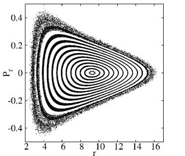
Figure 1: A 2D projection of a Poincaré section on the $r,~{}P_{r}$ plane for spins $a=0.9,~{}S=1$ and $H=0.95,~{}J_{z}=2$.

III.3 Examples for $S=1$

In order to find chaos we use the extreme case of $S=1$ in our first example. Fig. 1 shows a two dimensional projection of a Poincaré section. We can observe a chaotic region (scattered points) encircling an island of stability. The chaotic sea is confined between two surfaces. The inner one, which defines the limit of the island of stability, is a KAM torus, while the outer one is the boundary of the allowed motion. The outer boundary is indicated by the outer limit of the chaotic orbit. The boundary of the allowed motion has an opening around $r=2,~{}P_{r}=0$ from which the chaotic orbits are plunging towards the central black hole $(r=0)$. However, our observations are not unambiguous, since we do not see a Poincaré section in Fig. 1, but a projection. A 2D Poincaré section is accurate only for a Hamiltonian system of two degrees of freedom. In a two degrees of freedom system the KAM curves have zero width, and chaotic regions are represented by scattered dots covering a nonzero width region. In Fig. 1 we see KAM tori projected on a 2D plane, so the width of the KAMs is nonzero. Thus, a 2D Poincaré projection does not offer an unambiguous criterion to distinguish chaos from order. In order to drive safe conclusions we have to use 4D Poincaré sections.

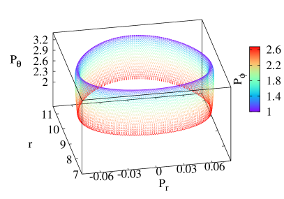
Figure 2: A regular torus from Fig. 1 with initial $r=7.5$ on a 4D Poincaré section.

Using the technique of color and rotation on a 4D Poincaré section, the regularity of an orbit in the neighborhood of a stable periodic orbit is indicated in the topology of the 3-dimensional projection by the presence of a torus, with a smooth color variation on its surface. This is determined by the distribution of the consequents in the 4th dimension Patsis94 . We use the orbit starting from $r=7.5$ in Fig. 1 to give our first example of a regular orbit on a 4D Poincaré section (Fig. 2). In Fig. 2 we observe that as the orbit evolves on the rotational torus projected on the $r,~{}P_{r},~{}P_{\theta}$ surface, the colors representing $P_{\phi}$ vary smoothly Katsanikas11a . This means that the orbit is regular. We use the software package “gnuplot” to visualize our results. We give the viewing angles of the 3D projections for Fig. 2 and all the subsequent similar figures of our paper in Table 1.

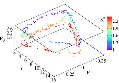
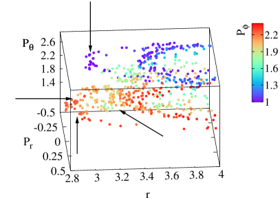
Figure 3: A chaotic orbit with initial $r=3,~{}P_{r}=0$ in Fig. 1 depicted in a 4D Poincaré section. The left plot shows the initial $300$ crossings of the orbit through the Poincaré section, while the right shows a detail from the Poincaré section when $1500$ crossings have been reached. The arrows indicate consequents almost on the surface that separates the allowed from the non-allowed space for the motion of the particle. For further explanations see text.

On a 4D Poincaré section the chaotic nature of an orbit is demonstrated by its irregular behavior on the 3-dimensional projection or/and by the mixing of colors representing the 4th dimension. In Fig. 3 we consider the chaotic orbit starting from $r=3$ on the 2D projection in Fig. 1. Initially the orbit sticks around a KAM lying on the border of the island of stability (This is given in the left plot of Fig. 3). By sticking around the torus it mimics a regular orbit (the color variation is smooth), but as the orbit evolves it departs from the KAM torus and sticks on the surface that defines the space for the allowed motion. The consequents of the orbit exhibit a smooth color variation. This is typical of the phenomenon of stickiness and it is quite common for weakly chaotic orbits, which are called sticky, see, e.g., Katsanikas11a . The arrows at the right plot in Fig. 3 show points that stick in this case on the outer boundary. The chaotic nature of the orbit is defined by its irregular behavior, and not by the color mixing. The orbit, after 1500 consequents, does not form a torus with small color variation on it like in Fig. 2, but it has a double loop structure. The fact that we do not have color mixing indicates stickiness Katsanikas13 . This behavior is similar to a weakly chaotic orbit that is trapped between two invariant curves in the case of a 2D Hamiltonian System.

III.4 Examples for $S=\sqrt{0.1}$

Figure 4: A detail from a 2D projection of a Poincaré section on the $r,~{}P_{r}$ plane for spins $a=0.9,~{}S=\sqrt{0.1}$ and $H=0.95,~{}J_{z}=2$.

We keep the same energy and angular momentum as in Sec. III.3, but we reduce the spin measure to $S=\sqrt{0.1}$. In this case a 2D projection of the whole phase space like the one in Fig. 1 is hardly discernible from a proper Poincaré map coming from a system with 2 degrees of freedom. One has to focus on a small region of the phase space to see the real structure (Fig. 4). In Fig. 4 we observe that there is still a chaotic region surrounding the main island of stability (scattered points on the left side of the plot), and that the KAM tori have nonzero width. It is worth mentioning that in a system of 3 degrees of freedom the chaotic regions communicate even if we see KAMs between them in the 3D projections of the 4D space of section. On the contrary in 2 degrees of freedom systems, when a KAM is lying between two chaotic regions in the 2D surface of section it does not allow them to communicate. A case where the two chaotic regions communicate is given in Fig. 4. Apart from the outer chaotic region there is a chaotic region lying on the interval $2.35\lesssim r\lesssim 2.37$. This region is inside the KAM tori that are lying on the interval $2.24\lesssim r\lesssim 2.25$ on the $P_{r}=0$ line in Fig. 4. By starting integrating an orbit in the inner chaotic region we soon end up in the outer one, since the two regions communicate.

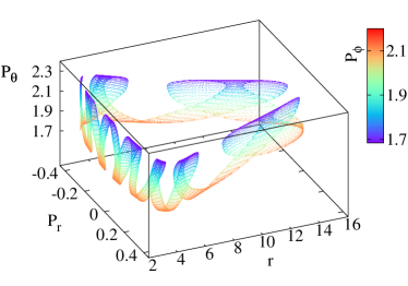
Figure 5: A regular torus from Fig. 4 with initial $r=2.4$ on a 4D Poincaré section.

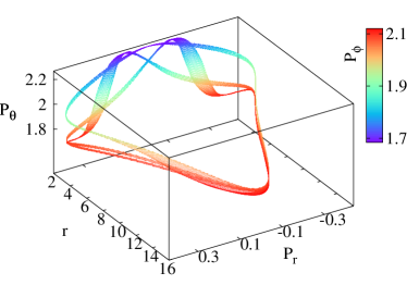
Figure 6: Filament corresponding to a chaotic orbit from Fig. 4 with initial $r=2.32$ on a 4D Poincaré section. The consequents after long integration time diffuse i phase space.

Actually the structure of the phase space is far more complicated. An example is a regular orbit, starting from $r=2.4$ which is represented by a structure that looks like nooses in a row in the 2D subspace $(r,P_{r})$ of the 4D Poincaré section (Fig. 4). This regular orbit is represented by a warped rotational torus on the 4D Poincaré section (see, e.g., Vrahatis97 , Katsanikas11a ). In Fig. 5 we see the real structure of the warped rotational torus. The regular orbit follows the warping of the torus while the color varies smoothly during the time of integration. On the other hand, weakly chaotic orbits lie in the region which is apparently dominated by KAM tori ($2.24\lesssim r\lesssim 2.25$ in Fig. 4). In Fig. 6 we plot such a weakly chaotic orbit. It is represented by a 3D filamentary structure with self-intersections in the 3D subspace $(r,P_{r},P_{\theta})$ of the 4D space of section. We observe that this structure has smooth color variation and that we have the same color (the same value in the 4th dimension) at the regions of the self-intersections.

We underline the fact that in Fig. 6 we observe two self-intersections that do not have the same color. If we rotate the figure, we can see these self-intersections from different viewing angles and we can observe very easily that these self-intersections do not exist in the 3D subspace. This means that these self-intersections are due to the viewing angles and they do not really exist. The smooth color variation of the 3D filamentary shows that the 4th dimension supports the geometry of this structure in the 4D space of section. This also gives us the dynamical information that these self-intersections occur in the 4D space. Such 4D filamentary structures have been encountered for the first time in a 3D galactic Hamiltonian system in Katsanikas11c and they are found at the neighborhood of unstable periodic orbits with high multiplicity Katsanikas11c . The orbits that are represented by these structures are sticky chaotic orbits.

Such weakly chaotic orbits have as a 2D counterpart the chaotic orbits that can be found in chains of elliptic and hyperbolic points in resonance zones. These chaotic orbits connect the hyperbolic points and surround the islands of stability of the elliptic ones. In the case we study here, these weakly chaotic orbits extend into the 3D space of the projection, while they have a smooth color variation along the filament they form. However, if we continue the integration for long times, the orbit will diffuse in the 4D space, something that will be demonstrated clearly in the next example.

III.5 Examples for $S\leq 0.1$

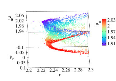
Figure 7: A detail from a 4D Poincaré section of a filamentary chaotic orbit with $S=0.1$ starting from $r=2.225$.

If we reduce the spin measure to $S=10^{-1}$ and $S=10^{-2}$, we encounter again 4D tori and 4D filamentary structures in the 4D space of section that correspond to regular orbits and sticky chaotic orbits respectively. In Fig. 7 (for $S=0.1$) we observe a 4D filamentary structure. Despite the fact that we have smooth color variation for the 4th dimension $P_{\phi}$ the consequents depart from this filamentary structure through the 3D subspace $(r,P_{r},P_{\theta})$, and they occupy larger volumes in the phase space (before the final plunge towards the black hole). These consequents can be observed at the left side of Fig. 7. The departure of these points from the filamentary structure happens earlier than in the case described in Fig. 6. However, in both cases we observe stickiness on 4D Poincré sections in structures that correspond to chaotic zones around unstable periodic orbits with high multiplicity for the first time in a relativistic system.

Figure 8: A detail from a 2D projection of a Poincaré section on the $r,~{}P_{r}$ plane for spins $a=0.9,~{}S=0.001$ and $H=0.95,~{}J_{z}=2$.

The last significant imprints of chaos are found for $S=10^{-3}$. For such low value of spin the 2D projection of a Poincaré section shown in Fig. 8 is very close to what one would expect to see in a case of a system with 2 degrees of freedom. In Fig. 8, we see a chaotic zone (scattered points on the left side), and a KAM torus (orbit on the right side of the plot). We have to focus significantly on the surface of section in order to make apparent the chaotic zone and the width of the torus.

For spins $S\leq 10^{-4}$ the presence of chaos appears to be negligible, and if this is the case it can be practically ignored. Even non-integrability effects like the existence of islands of stability near resonances can be neglected for any practical reason as well. In few words the system is nearly integrable, in agreement with the recent findings of Ruangsri15 , where no traces of resonant orbits were found in a study of a the linearized in spin MP equations. It is worth reminding that $S\leq 10^{-4}$ is the upper limit for the EMRIs, and it is interesting to notice that this value is also the upper limit for which the orbits produced by the Hamiltonian approximation start to match the orbits produced by the MP equations with NW SSC LGSK .

Fig.	$\theta$	$\phi$
2	$47^{o}$	$349^{o}$
3 (left panel)	$36^{o}$	$144^{o}$
3 (right panel)	$136^{o}$	$84^{o}$
5	$46^{o}$	$66^{o}$
6	$44^{o}$	$148^{o}$
7	$60^{o}$	$88^{o}$

Table 1: The view points of the figures, which are depicting 4D Poincaré section, are given in spherical coordinates $(\theta,\phi)$ as defined in the gnuplot software package.

IV Discussion and conclusions

The method of color and rotation Patsis94 is used for the first time in a relativistic system. Until now this method was used in 3D galactic Hamiltonian systems (Katsanikas11a ; Katsanikas11b ; Katsanikas11c ; Patsis14a ; Patsis14b , the 3D circular restricted three body problem Geisel13 and a 4D symplectic map Zachilas13 . We encountered three types of orbits in our study, which, though studied in detail in a 3D galactic system Katsanikas11a ; Katsanikas11c , have never been investigated in other 3D systems in the framework of general relativity. These three types of orbits are:

1. The first type of orbits are the regular orbits. These orbits are represented on the 4D Poincaré spaces of section by 4D rotational tori Katsanikas11a ; Vrahatis97 . These tori have the topology of a regular torus in the 3D projections of the 4D Poincaré space of section. Some of them are smooth regular tori and few of them are warped. Nevertheless, all of them manifest smooth color variation on them.

2. The second type of orbits are chaotic orbits that initially stick on 4D rotational tori (on the 4D Poincaré section), before they diffuse in the phase space.

3. The third type of orbits are a special case of chaotic orbits. They are represented by 4D filamentary structures on the 4D Poincaré sections as in Katsanikas11c . These structures are in the neighborhood of unstable periodic orbits with high multiplicity. Such orbits are sticky chaotic orbits since their consequents leave the 4D filamentary structures after a longer time of integration.

In general we did not encounter strong chaos in the system, which would be manifested by color mixing on the 4D Poincaré sections. We encountered only weakly chaotic and sticky orbits. Moreover, we observe that chaotic motion seems to be insignificant, and its contribution to the overall dynamics can be probably be neglected, when the dimensionless spin becomes smaller than $S=10^{-4}$, i.e. when the value of the spin is in the astrophysical relevant interval for extreme mass ratio inspirals. However, from a dynamical point of view the inclusion of the particle’s spin in the motion of a small compact object is just one way to go from the integrable case of geodesic motion on a Kerr black hole background to a non-integrable system. For example, it is well known that rings and halos around black holes can induce chaotic motion (see, e.g., SemSuk ). The same effect takes place when the spacetime around the central supermassive object is described by a non-Kerr black hole (see, e.g., nonKerr ). Non-integrability can also originate from the self-force or from the inclusion of the quadrupole momentum to the Mathisson-Papapetrou equations. In few words, there are many reasons for a extreme mass ratio binary to be described by a non-integrable system. However, it is unclear to which extent the effects coming from the non-integrability can affect the motion of the small body.

Appendix A Visualizing 4D Poincaré sections

Several methods have been used for visualizing the 4D spaces of section:

1. 2D and 3D projections: In this method the points of an orbit are plotted in a 2D subspace Contopoulos89 ; Skokos97 , §2.11.11 in Contopoulos02 or in a 3D subspace Vrahatis96 ; Vrahatis97 of the 4D Poincaré space of section. This method has the disadvantage that the distribution of the points in the 4 dimensional space is lost. However, in many cases, thin structures resembling invariant curves in the 2D case indicate the presence of tori.

2. Stereoscopic Views: Stereoscopic views of a 3D subspace of the 4D Poincaré space of section are used in order to understand the topology of the 3D projections Froeschle70 ; Martinet81 ; Contopoulos82 of the figures. For this reason, two figures are needed, one for each eye of the observer. However, this method cannot give any information about the behavior of the orbit in the 4th dimension.

3. The Method of Slices: In this method Froeschle70 ; Froeschle72 2D slices for different values of the third dimension of a 4D Poincaré space of section are produced. The successive 2D figures help one to see the distribution of the points of an orbit in the 3D subspace of the 4D space of section. By using this method many figures are needed in order to understand the third dimension and the fourth dimension in the 4D space of section is absolutely lost. An improved version of this method has been demonstrated recently in Richter14 ; Lange14 . In this case 3D are used, instead of 2D, slices of the space of section and they can be rotated by using standard 3D graphics software. By doing so, one can better see the third dimension and “visualize” the fourth dimension of the 4D Poincaré space of section as well. The disadvantage of this version of the slices method is that the 3D slices can be very complicated and sometimes it is difficult to see directly the topology of the orbits in the 4D Poincaré space of section.

4. The Method of Color and Rotation: This method was introduced in Patsis94 and is applied in the present paper (see also our introduction). The method has the advantage that we can observe the 4D distribution of the points of an orbit without any change of the 3D geometry or the 3D topology of the orbit in the 4D Poincaré space of section.

References

- (1) P., Amaro-Seoane, S. Aoudia, S. Babak,P. Binétruy, E. Berti, A. Bohé, C. Caprini, M. Colpi, N. J. Cornish, K. Danzmann, J.-F. Dufaux, J. Gair, I. Hinder, O. Jennrich, P. Jetzer, A. Klein, R. N Lang, A. Lobo, T. Littenberg, S. T. McWilliams, G. Nelemans, A. Petiteau, E. K Porter, B. F. Schutz, A. Sesana, R. Stebbins, T. Sumner, M. Vallisneri, S. Vitale, M. Volonteri, H. Ward, B. Wardell, GW Notes 6, 4-110 (2013)
- (2) M. Mathisson, Acta Phys. Polonica 6, 163 (1937)
- (3) A. Papapetrou, Proc. R. Soc. London Ser. A 209, 248 (1951)
- (4) C. Møller, Annales de l’I. H. P. 11, 251 (1949)
- (5) F. A. E. Pirani, Acta Phys. Polonica 15, 389 (1956)
- (6) W. Tulczyjew, Acta Phys. Polonica 18, 393 (1959)
- (7) O. Semerák, Mon. Not. R. Astron. S. 308, 863 (1999)
- (8) K. Kyrian, and O. Semerák, Mon. Not. R. Astron. S. 382, 1922 (2007)
- (9) O. Semerák, and M. Šrámek, Phys. Rev. D 92, 064032 (2015)
- (10) L. F. Costa, C. Herdeiro, J. Natario and M. Zilhão, Phys. Rev. D 85, 024001 (2012).
- (11) S. Suzuki and K. Maeda, Phys. Rev. D 55, 4848 (1997)
- (12) M. D. Hartl, Phys. Rev. D 67, 024005 (2003)
- (13) M. D. Hartl, Phys. Rev. D 67, 104023 (2003)
- (14) W. Han, Gen. Rel. Grav. 40, 1831 (2008)
- (15) R. Rüdiger, Proc. R. Soc. London Ser. A 375, 185 (1981); 385, 229 (1982)
- (16) T. Hinderer, A. Buonanno, A. H. Mroué et. al, Phys. Rev. D 88,084005 (2013)
- (17) E. Barausse, E. Racine, and A. Buonanno, Phys. Rev. D 80, 104025 (2009)
- (18) T. D. Newton, and E. P. Wigner, Rev. Mod. Phys. 21, 400 (1949)
- (19) E. Barausse, and A. Buonanno, Phys. Rev. D 81, 084024 (2010)
- (20) D. Kunst, T. Ledvinka, G. Lukes-Gerakopoulos, and J. Seyrich, Phys. Rev. D 93, 044004 (2016)
- (21) G. Contopoulos, Proc. Math. Phys. Sc. 431, 183 (1990)
- (22) G. Contopoulos, and B. Barbanis Celest. Mech. Dyn. Astron. 59, 279-300 (1989)
- (23) M.N. Vrahatis, H. Isliker, and T.C. Bountis Int. J. Bif. Chaos 7, 2707-2722 (1997)
- (24) C. Froeschlé Astron. Astrophys. 4, 115-128 (1970)
- (25) L. Martinet, and P. Magnenat [1981] Astron. Astrophys. 96, 68-77 (1981)
- (26) G. Contopoulos, P. Magnenat, and L. Martinet Physica D 6, 123-136 (1982)
- (27) C. Froeschlé Astron. Astrophys. 16, 172-189 (1972)
- (28) S. Lange, M. Richter,F. Onken, A. Bäcker and R. Ketzmerick Chaos 24, 024409 (2014)
- (29) M. Richter, S. Lange, A. Bäcker and R. Ketzmerick Phys. Rev. E 89, 022902 (2014)
- (30) P. A. Patsis and L. Zachilas Int. J. Bif. Chaos 4, 1399-1424 (1994)
- (31) M. Katsanikas and P.A. Patsis Int. Journal Bif. Chaos 21, 467-496 (2011)
- (32) M. Katsanikas, P.A Patsis and G. Contopoulos Int. Journal Bif. Chaos 21, 2321-2330 (2011)
- (33) M. Katsanikas, P.A. Patsis and A.D. Pinotsis Int. Journal Bif. Chaos 21, 2331-2342 (2011)
- (34) M. Katsanikas, P.A Patsis and G. Contopoulos Int. Journal Bif. Chaos 23, 1330005 (2013)
- (35) P.A. Patsis and M. Katsanikas Mon. Not. R. Astron. Soc. 445, 3525-3545 (2014)
- (36) P.A. Patsis and M. Katsanikas Mon. Not. R. Astron. Soc. 445, 3546-3556 (2014)
- (37) G. Contopoulos Order and Chaos in Dynamical Astronomy, Springer-Verlag, New York Berlin Heidelberg (2002)
- (38) L.Zachilas, M. Katsanikas and P.A. Patsis Int. Journal Bif. Chaos 23, 1330023 (2013)
- (39) Christopher D. Geisel, Spacecraft Orbit Design in the Circular Restricted Three-Body Problem Using Higher-Dimensional Poincaré Maps, PhD Thesis, Purdue University, West Lafayette, Indiana, USA (2013)
- (40) G. Lukes-Gerakopoulos, J. Seyrich, and D. Kunst Phys. Rev. D 90, 104019 (2014)
- (41) Ch. Skokos, G. Contopoulos G. and C. Polymilis Celest. Mech. Dyn. Astron. 65, 223-251
- (42) M.N. Vrahatis , T.C. Bountis and M. Kollmann Int. J. Bif. Chaos 6, 1425-1437 (1996)
- (43) U. Ruangsri, S. J. Vigeland, and S. A. Hughes, arXiv:1512.00376
- (44) O. Semerák, and P. Suková, Mon. Not. R. Astron. Soc. 404, 545 (2010); 425, 2455 (2012); P. Suková, and O. Semerák, Mon. Not. R. Astron. Soc. 436, 978 (2013); V. Witzany, O. Semerák, and P. Suková, Mon. Not. R. Astron. Soc. 451, 1770 (2015)
- (45) G. Lukes-Gerakopoulos, T. A. Apostolatos and G. Contopoulos, Phys. Rev. D 81, 124005 (2010); G. Contopoulos, G. Lukes-Gerakopoulos and T. A. Apostolatos, Int. J. Bifurc. Chaos 21, 2261 (2011)