Exact Bethe ansatz spectrum of a tight-binding chain with dephasing noise

Abstract

We construct an exact map between a tight-binding model on any bipartite lattice in presence of dephasing noise and a Hubbard model with imaginary interaction strength. In one dimension, the exact many-body Liouvillian spectrum can be obtained by application of the Bethe ansatz method. We find that both the non-equilibrium steady state and the leading decay modes describing the relaxation at late times are related to the $\eta$-pairing symmetry of the Hubbard model. We show that there is a remarkable relation between the time-evolution of an arbitrary $k-$point correlation function in the dissipative system and $k$-particle states of the corresponding Hubbard model.

Introduction.– The coupling to the environment often has a non-negligible influence on a many-particle system, and may drive it to a non-equilibrium steady state (NESS), that is different from the ground or thermal equilibrium states. Within the so-called Markovian description, assuming that the internal bath dynamics is much faster than that of the system so there is no back action of the system onto its environment, one has a well defined mathematical description of open many-body systems in both classical and quantum contexts. In the quantum realm, the open system’s Liouvillian dynamics is described by the Lindblad master equation Breuer for the time-dependent density matrix. A standard way of analyzing the Lindblad equation is by means of perturbative methods perturbation ; DiehlKeldysh , but it is highly desirable to have exact solutions in specific representative cases. While NESSs have been constructed exactly in a number of cases, in both classical ASEPNESS and quantum settings Pros2008 ; Marko ; ProsenExact , solving the full dynamics, i.e. diagonalizing the Liouvillian, for any nontrivial many-body system is a formidable task. In the quantum case this has so far been possible only for noninteracting systems Pros2008 . On the other hand, in certain classical stochastic many body systems like the asymmetric simple exclusion processes, the full Markov chain can be diagonalized in terms of the Bethe ansatz. ASEPBA It is then natural to ask whether there are quantum many-body dissipative systems that are Bethe ansatz solvable.

In this Letter we present an exactly solvable dissipative many-body quantum system that is not equivalent to a free theory: a fermionic tight-binding model on a bipartite lattice with dephasing noise. In one spatial dimension this model is equivalent, up to boundary conditions, to a dephased spin-1/2 $XX$ chain. The model has applications to ultra-cold atoms in an optical lattice subjected to light scattering Sarkar14 , and to superconducting flux qubits coupled to a fluctuating electromagnetic environment qbits . The dissipation in the form of dephasing destroys the quantum coherence, i.e. off-diagonal density matrix elements in the Fock space basis. It is known that such models exhibit diffusive behavior Esp2005 ; Eis2011 .

Even though the Hamiltonian of our model is quadratic in fermion operators, the dissipative term leads to quartic terms in the effective evolution operator, which renders its diagonalization a non-trivial task. We put forward a simple unitary transformation, within the thermofield description thermo , that maps the Liouvillian superoperator of our model on an arbitrary bipartite lattice to the Hubbard Hamiltonian with imaginary interaction strength. In one spatial dimension this means that the entire machinery of the Bethe ansatz formalism bookHub is applicable: we can obtain the full Liouvillian spectrum by solving the Bethe-ansatz equations, as well as reconstruct the time-evolution of the density matrix by expanding it over the Bethe-ansatz wave-functions.

Dephasing model.– We consider dissipative many-body dynamics of free fermions on a bipartite lattice in the tight-binding approximation with Hamiltonian

$$H=\sum_{\langle j,k\rangle}(a_{j}^{\dagger}a_{k}+a^{\dagger}_{k}a_{j}).$$ (1)

Here $a_{j}^{\dagger}/a_{j}$ are fermionic creation/annihilation operators on site $j$, and $\langle j,k\rangle$ denote nearest-neighbour links connecting the two sublattices $A$ and $B$. The dissipative dynamics is described by the Lindblad equation $\frac{\partial\rho}{\partial t}=\mathcal{L}[\rho]$, where

$$\mathcal{L}[\rho]=-i[H,\rho]+\mathcal{D}[\rho],~{}\mathcal{D}[\rho]=\sum_{j}\left(2l_{j}\rho l_{j}^{\dagger}-\{l_{j}^{\dagger}l_{j},\rho\}\right).$$ (2)

The Lindblad operators are $l_{j}=\sqrt{2\gamma}a^{\dagger}_{j}a_{j}$. The derivation of this dissipation term follows the books Gardiner ; Breuer , or Ref. Sarkar14 in the optical lattice context. The dephasing strength $\gamma$ is a function of the laser intensity and detuning.

It is useful to express the generator of the time-evolution (Liouvillian) in the thermofield representation thermo . To that end we introduce a second set of fermionic operators $\tilde{a}_{j}^{\dagger}$ and $\tilde{a}_{j}$, which act on the density matrix by right multiplication Dzh2012 ; fermionicHS . The Liouvillian then takes the form

$$\mathcal{L}=-i\mathcal{H}+2\gamma\sum_{j}\left(2a^{\dagger}_{j}a_{j}\tilde{a}^{\dagger}_{j}\tilde{a}_{j}-a^{\dagger}_{j}a_{j}-\tilde{a}^{\dagger}_{j}\tilde{a}_{j}\right),$$ (3)

where $\mathcal{H}=H-\tilde{H}$ is the time-evolution generator of the closed system in the thermofield representation. We note that the total numbers of particles of each ‘flavour’ (non-tilde and tilde operators) $M_{1}=\sum_{j}a^{\dagger}_{j}a_{j}$, $M_{2}=\sum_{j}\tilde{a}^{\dagger}_{j}\tilde{a}_{j}$ are conserved during time-evolution, as is their sum $N=M_{1}+M_{2}$. In the following we will choose $M_{1}\equiv M$ and $N$ as good quantum numbers of our problem.

Transformation to imaginary Hubbard model.– We now perform a unitary transformation which flips the sign of the tilde-Hamiltonian

$${\mathcal{U}}=\prod_{j\in{A}}e^{i\pi\tilde{a}_{j}^{\dagger}\tilde{a}_{j}}=\prod_{j\in{A}}(1-2\tilde{a}_{j}^{\dagger}\tilde{a}_{j}).$$ (4)

In the transformed basis the generator of time-evolution can be written as the Hamiltonian of the Hubbard model at a finite chemical potential and imaginary interaction strength $u=i\gamma$

$$H_{\mathrm{Hubb}} \equiv i{\mathcal{U}}^{\dagger}\mathcal{L}{\mathcal{U}}=\sum_{\langle j,k\rangle;\sigma=\uparrow,\downarrow}\left(c^{\dagger}_{j,\sigma}c_{k,\sigma}+h.c.\right)+$$ (5)

$$+ 4u\sum_{j}n_{j,\uparrow}n_{j,\downarrow}-2u\sum_{j;\sigma=\uparrow,\downarrow}n_{j,\sigma}.$$

Here the fermionic operators for the spin-up and spin-down are related to the normal and tilde operators of the dephasing model by $c_{i,\uparrow}=a_{i}$, $c_{i,\downarrow}=\tilde{a}_{i}$, and $n_{j,\sigma}=c^{\dagger}_{j,\sigma}c_{j,\sigma}$. The imaginary-$u$ Hubbard model (5) exhibits an $SO(4)$ symmetry HL ; etaPair ; bookHub . The generators of the constituent $\eta$-pairing $SU(2)$ algebra are $\eta^{z}=\sum_{j}(n_{j,\uparrow}+n_{j,\downarrow}-1)$, $\eta^{+}=\sum_{j\in A}c^{\dagger}_{j,\downarrow}c^{\dagger}_{j,\uparrow}-\sum_{j\in B}c^{\dagger}_{j,\downarrow}c^{\dagger}_{j,\uparrow}=(\eta^{-})^{\dagger}$, and will play an important role in the following.

Steady State.– The NESS is characterized by the condition $\mathcal{L}\rho=0$. In the sector $L=N=2M$, where $L$ is the total number of sites, it is easy to read off the NESS in the Hubbard model representation

$$|{\rm NESS}\rangle=\big{(}\eta^{\dagger}\big{)}^{M}|0\rangle,$$ (6)

where $|0\rangle$ is the fermion vacuum defined by $c_{j,\sigma}|0\rangle=0$. Given that $H_{\rm Hubb}|0\rangle=0$, the $\eta$-pairing symmetry implies that the state (6) has zero eigenvalue as well and therefore is a steady state. $\eta$-pairing states like (6) attracted attention in the early nineties in relation to high-$T_{c}$ superconductivity, because they are exact eigenstates of the Hubbard Hamiltonian that display off-diagonal long-range orderetaPair . However, in the Hubbard model they can never be ground states. The corresponding state in the dissipative model is obtained by undoing the unitary transformation (4), and is of the form $\sum_{n_{j}\in\{0,1\}}|{n_{1},\ldots,n_{L}}\rangle_{\uparrow}\otimes|{n_{1},\ldots,n_{L}}\rangle_{\downarrow}$, where $|{n_{1},\ldots,n_{L}}\rangle$ run over all Fock states of one flavour. Hence the density matrix corresponding to the NESS is an identity operator and represents a completely mixed (infinite temperature) state.

Correlation function – wave-function duality.– The evolution of the expectation value of the operator $O$ obeys the equation

$$\frac{d\langle{O}\rangle}{dt}=\mathrm{tr}\left(\frac{d\rho}{dt}O\right)=\mathrm{tr}(\mathcal{L}[\rho]O).$$ (7)

A straightforward calculation (substituting the explicit form of $\mathcal{L}[\rho]$ in Eq. (7) and using cyclic permutation invariance under the trace) shows that the equation for the dissipative time-evolution of the $2k$-point correlation function

$$G^{m_{1}\ldots m_{k}}_{n_{1}\ldots n_{k}}(t)=\mathrm{tr}(a^{\dagger}_{m_{1}}\ldots a^{\dagger}_{m_{k}}a_{n_{1}}\ldots a_{n_{k}}\rho(t))$$

is given by the same equation as the evolution of the density matrix elements corresponding wave functions in the $2k$ particle sector $\Psi^{m_{1}\ldots m_{k}}_{n_{1}\ldots n_{k}}\equiv G^{m_{1}\ldots m_{k}}_{n_{1}\ldots n_{k}}$,

$$\rho(t)=\!\!\!\!\!\!\sum_{m_{1}\ldots m_{k}n_{1}\ldots n_{k}}\!\!\!\!\Psi^{m_{1}\ldots m_{k}}_{n_{1}\ldots n_{k}}(t)a^{\dagger}_{m_{1}}\ldots a^{\dagger}_{m_{k}}|{0}\rangle\langle{0}|a_{n_{1}}\ldots a_{n_{k}}.$$

This duality, combined with the integrability of the imaginary-$u$ Hubbard model, gives a simple way for calculating general correlation functions of the tight-binding model with dephasing.

It has been noted previously Eis2011 that a one dimensional tight-binding model with (different) dephasing gives rise to a closed system of equations for correlation functions up to a given order, but in our case the Bethe ansatz solvability makes the duality much more powerful.

Liouvillian spectrum in one dimension.– The fact that the interaction strength is purely imaginary does not spoil the algebraic integrability structure of the Hubbard model. In fact, the Bethe ansatz wave-functions (related to the system’s density matrix) and the Bethe ansatz equations (BAE) are simply obtained from the regular Hubbard model by taking the interaction strength to be imaginary. The BAE for our case read BetheHub :

$$e^{ik_{j}L}=F_{1}\prod_{\alpha=1}^{M}\frac{\Lambda_{\alpha}-\sin k_{j}+\gamma}{\Lambda_{\alpha}-\sin k_{j}-\gamma},~{}j=1,\ldots,N,$$

$$\prod_{j=1}^{N}\frac{\Lambda_{\alpha}-\sin k_{j}+\gamma}{\Lambda_{\alpha}-\sin k_{j}-\gamma}=F_{2}\prod_{\beta,\beta\neq\alpha}\frac{\Lambda_{\beta}-\Lambda_{\alpha}+2\gamma}{\Lambda_{\beta}-\Lambda_{\alpha}-2\gamma},~{}$$ (8)

$$\alpha=1,\ldots,M.$$

Here $k_{j}$ and $\Lambda_{\alpha}$ are rapidities corresponding to charge and spin excitations, and we have introduced phase factors $F_{1,2}$ for later convenience. In the case at hand we have $F_{1}=F_{2}=1$. The eigenvalues of the Liouvillian ${\cal L}\rho_{\epsilon}=\epsilon\rho_{\epsilon}$ corresponding to a given solution of the Bethe equation $\{k_{j}\}$ are

$$\epsilon(\{k_{j}\})=-2i\sum_{j=1}^{N}\cos k_{j}-2N\gamma.$$ (9)

While the BAE allow us in principle to determine the full spectrum of the Liouvillian, we will be mainly interested in the structure of the slowest decaying NESS-excitations NESSExcitation , i.e. eigenvalues with the largest real parts.

Spectral properties of the Hubbard Hamiltonian are commonly analyzed in the framework of the so-called string hypothesisTakahashibook ; Takahashi ; bookHub , which assumes that, up to corrections that are exponentially small in system size, the roots of all solutions form particular “string” patterns in the complex plane. The structure of solutions of the imaginary-$u$ BAE is substantially different than in the usual Hubbard model. Interestingly, there exists a class of string solutions involving both $k$’s and $\Lambda$’s and is important for describing the late time behavior. A single such “$k$-$\Lambda$ string” of length $m$ consists of $2m$ charge rapidities $k^{(m)}_{\alpha,j}$ and $m$ spin rapidities $\Lambda_{\alpha,j}^{(m)}$ such that for $\lambda^{(m)}_{\alpha}<0$

$$k^{(m)}_{\alpha,j} = \arcsin(i\lambda^{(m)}_{\alpha}-(m-2j+2)\gamma),$$

$$k^{(m)}_{\alpha,j+m} = \pi-\arcsin(i\lambda^{(m)}_{\alpha}+(m-2j+2)\gamma),$$

$$\Lambda^{(m)}_{\alpha,j} = i\lambda^{(m)}_{\alpha}+\gamma(m+1-2j),~{}1\leq j\leq m.$$ (10)

For positive $\lambda^{(m)}_{\alpha}>0$ the structure of the string solution is the same as (10) with the replacement $\gamma\rightarrow-\gamma$. We stress that (10) are quite distinct from $k$-$\Lambda$-strings in the usual Hubbard model bookHub : the string centers are imaginary rather than real, and the $k$’s enter as pairs ($k$, $\pi+k^{*}$) rather than as ($k$, $k^{*}$). An example of a $k$-$\Lambda$ string solution in our model is shown in the left inset of Fig. 1. In the usual Hubbard model a $k$-$\Lambda$-string of length $m$ is a multi-particle bound state of $m$ fermions with spin up and $m$ fermions with spin down bookHub ; Essl1992 . In the present context $k$-$\Lambda$ string solutions to the BAE correspond to density matrices of our open system, that have exponentially decaying off-diagonal matrix elements. For example, in the sector $N=2M=2$ the NESS-excitations $\mathcal{L}\rho_{m}=\epsilon_{m}\rho_{m},~{}\rho_{m}=\rho_{m}^{\dagger}$ can be represented as $\rho_{m}=\sum_{x_{1},x_{2}}\rho_{m}(x_{1},x_{2})|{0\ldots 1_{x_{1}}\ldots 0}\rangle\langle{0\ldots 1_{x_{2}}\ldots 0}|$, where $\rho_{m}(x_{1},x_{2})=\begin{cases}f(x_{1},x_{2}),~{}x_{1}\geq x_{2},\\ -f(x_{1},x_{2}),~{}x_{1}<x_{2}\end{cases}$ with

$$f(x_{1},x_{2})=i^{2(x_{1}-x_{2})}(w+(-1)^{x_{1}+x_{2}}w^{*})e^{-\xi_{m}|x_{1}-x_{2}|},$$

$w=e^{-iq_{m}(x_{1}+x_{2})}$ and $q_{m}=\pm\frac{\pi m}{L}$, $\xi_{m}=\mathrm{arccosh}\frac{\gamma}{\sin q_{m}}$, $1\leq m\leq\frac{L}{2}$.

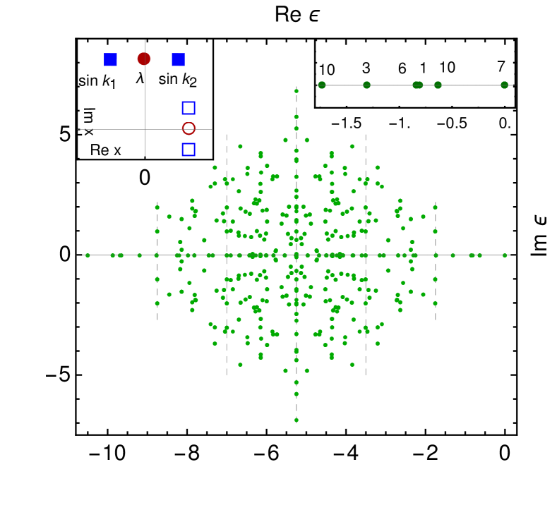
Figure 1: Spectrum of the tight-binding model with dephasing for $L=6$, $2\gamma=1.75$. Vertical dashed lines indicate multiples of $-2\gamma$. As a result of the $\mathbb{P}\mathbb{T}$-symmetryPT of the Liouvillian the spectrum exhibits a $D_{2}$ point symmetry. Left inset: Schematic representation of the $1k\Lambda$-string solution of the Bethe equations, for the imaginary $u$-Hubbard model (full symbols), and for the usual Hubbard chain with real $u$ (empty symbols). Right inset: Close-up of the slowest decaying modes. The numbers indicate the degeneracies, which are consistent with translation from the lower to higher magnetization sectors via the $\eta$-symmetry. For example, $10=5\cdot 2$ is obtained by counting the number of $\eta$-pairing descendant states in sectors with higher numbers of particles (there are $L-1=5$), while the factor of $2$ is due to a degeneracy in the sector $N=2$, $M=1$ of $\eta$-pairing lowest weight states, which is a consequence of the parity symmetry of the Hamiltonian (5). The non-degenerate state shown has $N=2M=6$ and is a singlet both with respect to parity and the $\eta$-pairing.

For the particular subset of solutions of (8) that consists only of $k$-$\Lambda$ strings we may use the string hypothesis (10) to obtain the following set of equations for the string centers $\lambda^{(n)}_{\alpha}$

$$Lf_{m}(\lambda^{(m)}_{\alpha})=2\pi J^{(m)}_{\alpha}+\sum_{(m,\beta)}\Theta_{nm}\Big{(}\frac{\lambda^{(m)}_{\alpha}-\lambda^{(n)}_{\beta}}{\gamma}\Big{)}\ .$$ (11)

Here $f_{m}(x)={\rm sgn}(x)\big{(}\pi-{\rm arcsin}(ix+m\gamma)+{\rm arcsin}(ix-m\gamma)\big{)}$, and $\Theta_{nm}(x)=2\theta(x/|n-m|+2)+\dots+2\theta(x/n+m-2)+\theta(x/n+m)+(1-\delta_{n,m})\theta(x/|n-m|)$ with $\theta(x)=2{\rm arctan}(x)$ is the same function as in the usual Hubbard model. The (half-odd) integers $J^{(m)}_{\alpha}$ have ranges $|J^{(m)}_{\alpha}|\leq\frac{L-1}{2}-\frac{1}{2}\sum_{n=1}\big{(}2{\rm min}(m,n)-\delta_{m,n}\big{)}M_{n}$. Here $M_{n}$ is the number of $k$-$\Lambda$ strings of length $n$, and $N=2M=\sum_{n=1}^{\infty}2nM_{n}$. The corresponding eigenvalues of the Liouvillian are real and given by

$$\epsilon = 4\sum_{(m,\alpha)}{\rm Im}\sqrt{1-(i|\lambda^{(m)}_{\alpha}|-m\gamma)^{2}}-2\gamma N.$$ (12)

Moreover, studies of small systems $L\leq 8$ strongly suggest that $k$-$\Lambda$ string solutions and their $\eta$-pairing descendant states provide all slowly decaying NESS-excitations. In Fig. 1 we show the full spectrum of $\mathcal{L}$ for $L=6$. The states with ${\rm Re}(\epsilon)>-2\gamma$ are all given by $k$-$\Lambda$ string solutions and their $\eta$-pairing descendants, cf. the right inset of Fig. 1. The situation for $L=8$ is analogous. Assuming this to hold in general, we can obtain the eigenvalues of $\mathcal{L}$ with the largest real parts (i.e. the eigenvalues closest to zero) from the equations (11) for the string centers. For solutions consisting of a single $k$-$\Lambda$ string $n$, i.e. $M_{n}=1$, $M_{j\neq n}=0$, we find a sequence of eigenvalues with

$$\epsilon_{n,j}=-\frac{1}{\gamma}\cdot\frac{2\pi^{2}(n+j-1)^{2}}{nL^{2}}+{\cal O}(L^{-4})\ ,\ j\in\mathbb{N}^{+},$$ (13)

where we have assumed $n,|j|\ll L$. Let us denote the corresponding eigenstates by $|n,j\rangle$. Using the $\eta$-pairing symmetry we can construct degenerate states in the sector $N=2M=2k+2n$ of the form

$$(\eta^{\dagger})^{k}|n,j\rangle\ .$$ (14)

This shows that the spectrum of the dephasing model is gapless in the thermodynamic limit in any magnetization sector. For large but finite $L$ the smallest gap is given by $\epsilon_{1,1}$. The above construction carries over to general nonintegrable bipartite lattices in the sense that NESS-excitations can be constructed from two-particle states by acting with an appropriate power of $\eta^{\dagger}$. In contrast to the usual Hubbard model unstableEtaPair , perturbation theory in $1/\gamma$ suggests that $\eta$-pairing NESS-excitations are stable to typical perturbations in the sense that they do not couple to states in the complex part of the spectrum and retain real eigenvalues.

Large $\gamma$ limit.– It is known that in the limit of strong dephasing $\gamma\gg 1$ the late time dynamics of our system is described by a classical stochastic process on the space of the diagonal density matrices, with an evolution operator that is equivalent to Hamiltonian of the spin-1/2 Heisenberg chain Cai . This relation implies that the NESS-excitations are gapless in any space dimension, as the lowest lying excitation of the ferromagnet are gapless. We have already commented that the $k$-$\Lambda$ solutions describing the longest living NESS-excitations have exponentially decaying off-diagonal matrix elements (they decay exponentially away from diagonal with a scale determined from the solution of the BAE). In the large $\gamma$ limit further simplifications occur. In particular the BAE (11) reduce to Takahashi’s equations for the spin-1/2 Heisenberg ferromagnet: Takahashibook rescaling the rapidities $\lambda^{(m)}_{\alpha}=\gamma\mu^{(m)}_{\alpha}$ and then taking $\gamma\to\infty$ gives

$$L\theta(\mu^{(m)}_{\alpha}/m) = 2\pi J^{(m)}_{\alpha}+\sum_{(m,\beta)}\Theta_{nm}\big{(}{\mu^{(m)}_{\alpha}-\mu^{(n)}_{\beta}}\big{)}\ ,$$

$$\epsilon = -\frac{1}{\gamma}\sum_{(m,\alpha)}\frac{2m}{m^{2}+(\Lambda^{(m)}_{\alpha})^{2}}.$$ (15)

The emergence of an effective description in terms of a Heisenberg ferromagnet in the large-$\gamma$ regime of the dissipative model should be contrasted to the large-$u$ expansion in the real-$u$ Hubbard model. Indeed, the low energy manifold for the Hubbard model with large real interaction strength consists of configurations with zero or one fermion per site only, while for the strongly dissipative case the allowed configurations are those with zero or two fermions per site (corresponding to the mostly diagonal density matrices). The analogue of the large-$u$ expansion in the dissipative case gives access to rapidly decaying modes with $\epsilon\approx-2\gamma N$.

Relaxation dynamics.– It has been shown Esp2005 ; Eis2011 that in the sector $N=2,~{}M=1$ the relaxation dynamics is diffusive, both by means of spectral considerations Esp2005 and by studying the decay Eis2011 $\langle 2a^{\dagger}_{1}a_{1}-1\rangle\propto t^{-1/2}$ of an initially localized excitation $\langle 2a^{\dagger}_{j}a_{j}-1\rangle_{t=0}=\delta_{j,1}$ DecayExplan . By considering the off-diagonal elements of the density matrix and using the duality between the density matrices and correlation functions, one can easily calculate the decay of coherences in the many-particle states of the tight-binding model and obtain the dependence $\sim t^{-3/2}$ (similar to a numerical result for the coherences in the $XXZ$ model with dephasing obtained in Ref. Cai, ). The long time relaxation of many-particle states is influenced by the bound-state-like NESS-excitations.

XX model with dephasing.– Most of our results apply also to the spin-1/2 $XX$ chain with dephasing $H^{\mathrm{XX}}=\tfrac{1}{2}\sum_{j}^{L}(\sigma^{+}_{j+1}\sigma^{-}_{j}+\sigma^{+}_{j}\sigma^{-}_{j+1})$, $l^{\mathrm{XX}}_{j}=\sqrt{\gamma/2}\sigma^{z}_{j}$, where $\sigma^{+},\sigma^{-},\sigma^{z}$ are Pauli spin matrices. The $XX$ chain can be mapped to a tight-binding model with dephasing by means of a Jordan-Wigner transformation, but we now have to impose periodic/antiperiodic (p/a) boundary conditions in the even/odd magnetization sectors.bookNagaosa Proceeding as before we eventually arrive at an imaginary-$u$ Hubbard Hamiltonian (5). However, spin-$\sigma$ fermions now have periodic (antiperiodic) boundary conditions, if their total number is even (odd). Altogether we therefore have four distinct sectors (p,p), (p,a), (a,p), (a,a). As a consequence of this the imaginary-$u$ Hubbard Hamiltonian does not exhibit the full $SO(4)$ symmetry, but as $(\eta^{+})^{2}$ acts within a given sector, it commutes with the Hamiltonian. In spite of the changed boundary conditions the model remains integrable. The BAE are again of the form (8), but we now have $F_{1}=(-1)^{N-M-1}$, $F_{2}=(-1)^{N}$. Low-lying excitations can again be analyzed by means of the string hypothesis (10) and the equations (11) for the string centers. The main difference to the dissipative tight-binding model is that in the $XX$ case there is no closed form expression for the expectation values of the $k$-point spin correlations functions, as the spins are non-local in terms of Jordan-Wigner fermions.

Generalization to open boundaries.– If in addition to dephasing there is influx/outflux of particles on the boundary sites, i.e. there are additional Lindblad operators $l_{1,2}=a_{1,L}^{\dagger},~{}l_{3,4}=a_{1,L}$, or $l^{\mathrm{XX}}_{1,2}=\sigma^{+}_{1,L},~{}l^{\mathrm{XX}}_{3,4}=\sigma^{-}_{1,L}$, the Liouvillian in the thermofield language has the form of the Hubbard model with imaginary interaction and with an imaginary boundary magnetic field. The resulting model is again Bethe ansatz solvable Chineese . We note that the current-carying NESS of such a model has a simple explicit matrix product form Marko .

Conclusions.– We have shown that a dissipative tight-binding model on a bipartite lattice can be mapped to a Hubbard model with imaginary interaction strength. The NESS and the relaxational dynamics at late times is related to the $\eta$-pairing symmetry of the Hubbard model. In one spatial dimension we have used the Bethe ansatz solution to derive exact results on the spectrum of the Liouvillian. Our result pave the way to further studies of Bethe ansatz solvable quantum dissipative systems.

This work was supported by the Slovenian Research Agency (ARRS) under grants J1-5439 and N1-0025, the ERC grant OMNES (MVM and TP), and by the EPSRC under grant EP/N01930X. FHLE and TP thank the Isaac Newton Institute for Mathematical Sciences for hospitality and support under grant EP/K032208/1. MVM is greatful to Marko Medenjak for numerous discussions.

References

- (1) H.-P. Breuer and F. Petruccione, The Theory of Open Quantum Systems, Ch.3.5, p. 166, Oxford University Press, 2002.
- (2) A. C. Y. Li, F. Petruccione and J. Koch, Perturbative approach to Markovian open quantum systems, Sci. Rep. 4, 4887 (2014).
- (3) L. M. Sieberer, M. Buchhold and S. Diehl, Keldysh Field Theory for Driven Open Quantum Systems, arXiv:1512.00637.
- (4) B. Derrida, E. Domany, D. Mukamel, An exact solution of the one dimensional asymmetric exclusion model with open boundaries, J. Stat. Phys. 69, 667 (1992); B. Derrida, M. R. Evans, V. Hakim, and V. Pasquiert, Exact solution of a ID asymmetric exclusion model using a matrix formulation, J. Phys A: Math. Gen. 26 1493 (1993); R. A. Blythe and M. R. Evans, Nonequilibrium steady states of matrix-product form: a solver’s guide, J. Phys. A: Math. Theor. 40, R333 (2007).
- (5) T. Prosen, Third quantization: a general method to solve master equations for quadratic open Fermi systems, New J. Phys 10, 043026 (2008).
- (6) M. Žnidarič, Exact solution for a diffusive nonequilibrium steady state of an open quantum chain, J. Stat. Mech. L05002 (2010); Solvable quantum nonequilibrium model exhibiting a phase transition and a matrix product representation, Phys. Rev. E 83, 011108 (2011).
- (7) T. Prosen Exact Nonequilibrium Steady State of a Strongly Driven Open XXZ Chain, Phys. Rev. Lett. 107, 137201 (2011); Exact Nonequilibrium Steady State of an Open Hubbard Chain, Phys. Rev. Lett. 112, 030603 (2014); T.Prosen, Matrix product solutions of boundary driven quantum chains, J. Phys. A: Math. Theor. 48, 373001 (2015).
- (8) L.-H. Gwa and H. Spohn, Six-vertex model, roughened surfaces, and an asymmetric spin Hamiltonian, Phys. Rev. Lett. 68, 725 (1992); L.-H. Gwa and H. Spohn, Bethe solution for the dynamical-scaling exponent of the noisy Burgers equation, Phys. Rev. A 46, 844 (1992); D. Kim, Bethe ansatz solution for crossover scaling functions of the asymmetric XXZ chain and the Kardar-Parisi-Zhang-type growth model, Phys. Rev. E 52, 3512 (1995); O. Golinelli and K. Mallick, Bethe ansatz calculation of the spectral gap of the asymmetric exclusion process, J. Phys. A 37, 3321 (2004); J. de Gier and F.H.L. Essler, Bethe Ansatz Solution of the Partially Asymmetric Exclusion Process, Phys. Rev. Lett. 95, 240601 (2005); J. de Gier and F.H.L. Essler, Exact Spectral Gaps of the Asymmetric Exclusion Process with Open Boundaries, J. Stat. Mech. P12011 (2006); J. de Gier and F.H.L. Essler, Slowest Relaxation Mode of the Partially Asymmetric Exclusion Process with Open Boundaries, J. Phys. A41, 485002 (2008); K. Mallick, Some exact results for the exclusion process, J. Stat. Mech. P01024 (2011); N. Crampe, E. Ragoucy and D. Simon, Matrix coordinate Bethe Ansatz: applications to XXZ and ASEP models, J. Phys. A: Math. Theor. 40, 405003 (2011).
- (9) S. Sarkar, S. Langer, J. Schachenmayer, and A. J. Daley, Light scattering and dissipative dynamics of many fermionic atoms in an optical lattice, Phys. Rev. A 90, 023618 (2014).
- (10) J. E. Mooij, T. P. Orlando, L. Levitov, L. Tian, C. H. van der Wal, and S. Lloyd, Josephson Persistent-Current Qubit, Science 285, 1036 (1999).
- (11) M. Esposito, and P. Gaspard Exactly solvable model of quantum diffusion, J. Stat. Phys. 121, 463 (2005).
- (12) V. Eisler, Crossover between ballistic and diffusive transport: the quantum exclusion process, J. Stat. Mech. P06007 (2011).
- (13) H. Umezawa, Advanced Field Theory: Micro, Macro and Thermal Physics, AIP Press, New York (1993).
- (14) F. H. L. Essler, H. Frahm, F. Göhmann, A. Klümper, V. E. Korepin, The One-Dimensional Hubbard Model, Cambr. Univ. Press, 2005.
- (15) C. W. Gardiner and P. Zoller, Quantum Noise, Ch.3.6, p. 77, Springer, 1991.
- (16) A. A. Dzhioev, D. S. Kosov, Nonequilibrium perturbation theory in Liouville-Fock space for inelastic electron transport, J. Phys.: Cond. Matt. 24, 225304 (2012).
- (17) Let us note that in general fermionic models in the double channel representation have a more complicated structure of the Hilbert space compared to the spin systems. The obtained simple form of the dissipator is due to simple form of the Lindblad operators: they conserve the particle number and are quadratic.
- (18) O. J. Heilmann and E. H. Lieb, Violation of noncrossing rule — Hubbard Hamiltonian for benzene, Ann. N.Y. Acad. Sci. 172, 584 (1971).
- (19) C. N. Yang, -pairing and off-diagonal long-range order in a Hubbard model, Phys. Rev. Lett. 63, 2144 (1989); C. N. Yang and S. C. Zhang, symmetry in a Hubbard model, Mod. Phys. Lett. B 4, 759 (1990).
- (20) I. Fomin, P. Schmitteckert, and P. Wölfle, Comment on “Pseudospin symmetry and new collective modes of the Hubbard model”, Phys. Rev. Lett. 69, 214 (1992).
- (21) Elliott H. Lieb and F. Y. Wu, Absence of Mott Transition in an Exact Solution of the Short-Range, One-Band Model in One Dimension, Phys. Rev. Lett. 20, 1445 (1968).
- (22) NESS-excitations are defined as traceless and Hermitian linear combinations of the eigenoperators of the Liouvillian which have the same decay rate. The name excitation goes in analogy with excitations in the Hamiltonian dynamics, though for the Liouvillian the excitations are counted from the NESS, and not from the ground state. For more detail explanation of the term, see M. V. Medvedyeva and S. Kehrein, Power-law approach to steady state in open lattices of noninteracting electrons, Phys. Rev. B 90, 205410 (2014).
- (23) M. Takahashi, Thermodynamics of one dimensional solvable models, Cambridge University Press, Cambridge 1999;
- (24) M. Takahashi, Prog. Theor. Phys. 47, 69 (1972), One dimensional Hubbard model at finite temperature.
- (25) F. H.L. Essler, V. E. Korepin, K. Schoutens, Completeness of the SO(4) extended Bethe ansatz for the one-dimensional Hubbard model, Nucl. Phys. B, 384, 431 (1992).
- (26) T. Prosen, PT-Symmetric Quantum Liouvillean dynamics, Phys. Rev. Lett. 109, 090404 (2012).
- (27) Z. Cai and T. Barthel, Algebraic versus exponential decoherence in dissipative many-particle systems, Phys. Rev. Lett. 111, 150403 (2013).
- (28) Actually the decay of the single particle functions was derived in the Ref. Eis2011 for slightly different dissipators, but a simple calculation for our model gives the same.
- (29) N. Nagaosa, Quantum field theory in strongly correlated electronic systems, Springer, 1999.
- (30) Y.-Y. Li, J. Cao, W.-L. Yang, K. Shi, Y. Wang, Exact solution of the one-dimensional Hubbard model with arbitrary boundary magnetic fields, Nucl. Phys. B, 879, 98 (2014).