A Tale of Two Fractals: The Hofstadter Butterfly and The Integral Apollonian Gaskets

Abstract

This paper unveils a mapping between a quantum fractal that describes a physical phenomena, and an abstract geometrical fractal. The quantum fractal is the Hofstadter butterfly discovered in $1976$ in an iconic condensed matter problem of electrons moving in a two-dimensional lattice in a transverse magnetic field. The geometric fractal is the integer Apollonian gasket characterized in terms of a $300$BC problem of mutually tangent circles. Both of these fractals are made up of integers. In the Hofstadter butterfly, these integers encode the topological quantum numbers of quantum Hall conductivity. In the Apollonian gaskets an infinite number of mutually tangent circles are nested inside each other, where each circle has integer curvature. The mapping between these two fractals reveals a hidden $D_{3}$ symmetry embedded in the kaleidoscopic images that describe the asymptotic scaling properties of the butterfly. This paper also serves as a mini review of these fractals, emphasizing their hierarchical aspects in terms of Farey fractions.

1 Introduction

The Hofstadter butterflyAzbel ; Lan ; Hof as shown in Fig. 1 is a fascinating two-dimensional spectral landscape – a graph of allowed energies of an electron moving in a two-dimensional lattice in a traverse magnetic field. It is a quantum fractal madeup of integers. These integers are the topological quantum numbers associated with the quantum Hall effectQHE which is one of the most exotic phenomena in condensed matter physics. The basic experimental observation is the quantization of conductivity, in two-dimensional systems, to a remarkable precision , irrespective of the sample s shape and of its degree of purity. The butterfly graph as a whole describes all possible phases of a two-dimensional electron gas that arise as one varies the electron density and the magnetic field where each phase is characterized by an integer. These integers have their origin in topological properties described within the framework of geometric phases known as Berry phasesBerry . The relative smoothness of colored channels in Fig. 1 that describe gaps or forbidden energies of electrons is rooted in the topological characteristics of the butterfly graph.

The order and complexity of the butterfly shows how nature reacts to a quantum situation where there are two competing length scales. These are the periodicity of the crystalline lattice and the magnetic length representing the cyclotron radius of electrons in the magnetic field. Discovered in $1976$ by Douglas Hofstadter, the butterfly spectrum, fondly referred to as the Hofstadter butterfly, continues to arouse a great deal of excitement and there are various recent attempts to capture this iconic spectrum in various laboratoriesEXPT .

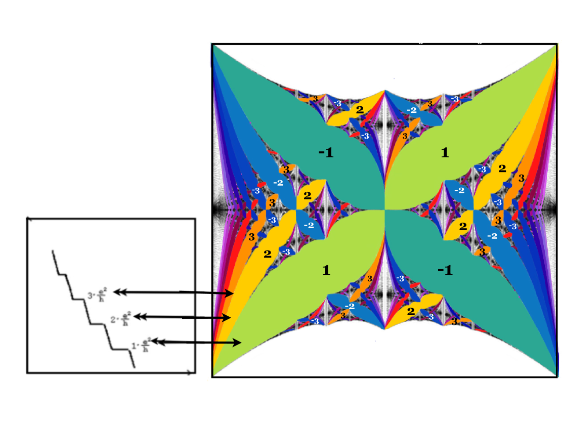
Figure 1: Left panel shows the schematic diagram of quantum Hall conductivity vs. magnetic field, showing plateaus at integer multiples of $\frac{e^{2}}{h}$. Here $e$ is the electron charge and $h$ is the Planck constant. On the right is the Hofstadter butterfly fractal where quantum mechanically forbidden values of energy – referred to as gaps are shown in various colors. Each gap is labeled by an integer (where only few are shown explicitly in the figure). The topological quantum number of Hall conductivity and gaps with same color highlight the fact that they are described by the same integer. Arrows point to the fact that different gaps of the butterfly represent different quantum Hall states.

The Fractal properties of the butterfly spectrum have been the subject of the various theoretical studiesWan Mac Wil . However, the universal scalings associated with self-similar nested set of butterflies has remained an open problem. Here we present a different perspective on the nesting behavior of this fractal graph as we study the recursive behavior of the butterflies – the extended two-dimensional structures, instead of the recursions at a fixed value of the magnetic flux, which has been the case in earlier studies. Using simple geometrical and number theoretical tools, we obtain the exact scalings associated with the magnetic flux interval that determines the horizontal size of the butterfly and their topological quantum numbers, as we zoom into smaller and smaller scale. The universal scaling associated with the energy intervals, namely the vertical size of the butterflies is obtained numerically.

The central focus here is the unveiling of the relationship between the Hofstadter butterfly and Integral Apollonian Gaskets ( $\cal{IAG}$ )IAG . $\cal{IAG}$ named in honor of Apollonius of Perga (before 300 BC), describe a close packing of circles. They are fascinating patterns obtained by starting with three mutually tangent circles and then recursively inscribing new circles in the curvilinear triangular regions between the circles. We show that the nested set of butterflies in the Hofstadter butterfly graph can be described in terms of $\cal{IAG}$. The key to this mapping lies in number theory, where butterfly boundaries are identified with a configuration of four mutually tangent circles. An intriguing result is the emergence of a hidden three-fold or $D_{3}$ symmetry of the associated Apollonians that are related in a subtle way to the butterfly spectrum. Underlying this hidden symmetry is an irrational number $2+\sqrt{3}$ whose continued fraction expansion is given by $[1,2,1,2,1,2...]$. In an analogy to the golden mean, we will refer to this irrational number as the diamond mean.

In this paper, we review various aspects of the butterfly spectrum and the $\cal{IAG}$ and describe the relationship between these two fractals. The discussion of the mapping between the butterfly and the $\cal{IAG}$ begins with an introduction to Ford circles, which are pictorial representations of rationals by circles as discovered by American mathematician Ford in $1938$Ford . The mathematics underlying the Apollonian-Butterfly connection ( $\cal{ABC}$) is encoded in Descartes’s theoremDT . Our presentation of $\cal{ABC}$ is empirical and the rigorous framework is currently under investigation. For further details regarding the Hofstadter butterfly and its relation to Apollonian gaskets, we refer readers to an upcoming bookkitab .

2 Model System and Topological Invariants

The model system we study here consists of electrons in a square lattice. Each site is labeled by a vector ${\bf r}=n\hat{x}+m\hat{y}$, where $n$, $m$ are integers, $\hat{x}$ ($\hat{y}$) is the unit vector in the $x$ ($y$) direction. The lattice with spacing $a$ is subjected to a uniform magnetic field $B$ along the $z$ direction, introducing a magnetic flux $Ba^{2}$ per unit cell of the lattice. In units of the flux quantum $\Phi_{0}$ (the natural unit of magnetic flux), the flux quanta per unit cell of the square lattice are denoted as $\phi=Ba^{2}/\Phi_{0}$. It turns out that $\phi$ is the key parameter that lies at the heart of the Hofstadter butterfly graph.

The quantum mechanics of this two dimensional problem can be described in terms of a one-dimensional equation, known as the Harper equationHof

$$\psi_{n+1}+\psi_{n-1}+2\cos(2\pi n\phi+k_{y})\psi_{n}=E\psi_{n}.$$ (1)

Here $\psi_{n}$ is wave function with energy $E$ of the election, subjected to the magnetic flux $\phi$.The parameter $k_{y}$ is related to the momentum of the electron.

The Butterfly graph (See right panel of Figs. 1 and also Fig. 2), is a plot of possible energies of the electron for various values of $\phi$ which varies between $[0,1]$. The permissible energies are arranged in bands separated by forbidden values, known as the gaps. In general, for a rational $\phi=\frac{p}{q}$, the graph consists of of $q$ bands and $(q-1)$ gaps. For an even $q$, the two central bands touch or kiss one another as illustrated in the left panel in Fig. 2.

It has been shown that the gaps of the butterfly spectrum are labeled by integers, which we denote as $\sigma$. These integers have topological origin and are known as Chern numbersQHE . They represent the quantum numbers associated with Hall conductivity: $C_{xy}=\sigma{e^{2}}/{h}$QHE as shown in the left panel in Fig. (1).

The mathematics underlying the topological character of the Chern numbers is closely related to the mathematical framework that describes Foucault’s pendulum. As the earth rotates through an angle of $2\pi$ radians the pendulum’s plane of oscillation fails to return to its starting configuration. Analogously, in the quantum Hall system, it is the phase of the wave function given by Eq. 1 that does not return to its starting value after a cyclic path in momentum space. Michael Berry himself put it as follows: “A circuit tracing a closed path in an abstract space can explain both the curious shift in the wave function of a particle and the apparent rotation of a pendulum’s plane of oscillation”. Chern numbers are the geometric phases in units of $2\pi$.

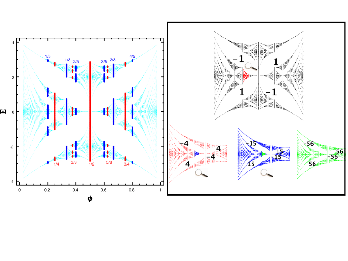
Figure 2: The left panel shows the butterfly plot for some rational values of the magnetic flux. For $\phi=p/q$, there are exactly $q$ bands (allowed values of energies) shown in the red (q-even) and blue (q-odd). Gaps in this plot are white regions resembling four wings of a butterfly. The figure on the right illustrates self-similar characteristics of the Hofstadter butterfly. Zooming into the butterfly fractal reveals similar patterns at all scales. The red butterfly is a blowup of the red region in the upper black graph. The blue butterfly is a blowup of the blue region in the red graph, and the green butterfly is, in turn, a blowup of the green region in the blue graph. The integers labeling the white gaps in these differently-colored butterflies are the quantum numbers of the Hall conductivity.

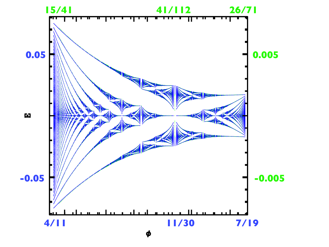
Figure 3: Two consecutive generations of butterflies, shown in blue and green (see also Fig. 2), overlaid. The blue labeling of the axes tells us where the blue butterfly is found, and likewise for the green labeling of the axes. This nearly perfect alignment illustrates the asymptotically exact self-similarity of the butterfly graph. The vertical or energy scale factor has so far been determined numerically and it is approximately $9.87\approx\pi^{2}$.

3 Butterfly Fractal

Figure (2) ( right panel) and Fig. (3) provide a visual illustration of self-similar fractal aspects of the butterfly graph. For simplicity, we will focus on those butterflies whose centers are located on the $x$-axis, namely at $E=0$. As we zoom into these centered “equivalent ” set of butterflies , we see same structure at all scales. We label each butterfly with the rational magnetic flux values at its center and its left and the right edges. Denoting this triplet as $(\frac{p_{L}}{q_{L}},\frac{p_{c}}{q_{c}},\frac{p_{R}}{q_{R}})$, we note the following:

1. For butterflies with center at $E=0$, the integer $q_{c}$ is always an even integer while $q_{L}$ and $q_{R}$ are odd.

2. For any butterfly, the locations of its center and its left and right edges are related to each other by the following equation:

   $$\frac{p_{c}}{q_{c}}=\frac{p_{L}+p_{R}}{q_{L}+q_{R}}\equiv\frac{p_{L}}{q_{L}}\bigoplus\frac{p_{R}}{q_{R}}$$ (2)

The above equation defines what is know as the “Farey sum”. It turns out that Farey tree where all irreducible rational numbers $\frac{p}{q}$ with $0\leq p\leq q\leq n$, are arranged in an increasing order, provides a useful framework to describe the butterfly fractal. In general, at any level of the Farey tree, two neighboring fractions $\frac{p_{1}}{q_{1}}$ and $\frac{p_{2}}{q_{2}}$ have the following property, known as the “friendship rule” .

$$p_{1}q_{2}-p_{2}q_{1}=\pm 1$$ (3)

We note that any two members of the butterfly triplet $(\frac{p_{L}}{q_{L}},\frac{p_{c}}{q_{c}},\frac{p_{R}}{q_{R}})$ satisfy Eq. (3) .

3.1 Butterfly Recursions

As we examine the entire butterfly graph at smaller and smaller scales, we note that there exists a butterfly at every scale, and the miniature versions exhibit every detail of the original graph. Since the nesting of butterflies goes down infinitely far, it is useful to define a notion of levels, or generations. The top level, or first generation, is the full butterfly stretching between $\phi=0$ and $\phi=1$, with its fourfold symmetry. We will say that butterflies A and B belong to successive generations when B is contained inside A and when there is no intermediate butterfly between them. Our discussion below includes only those cases where the larger and the smaller butterflies share neither their left edge nor their right edge. In this manner, any miniature butterfly can be labeled with a positive integer telling which generation it belongs to. We show that these class of butterflies are characterized by a nontrivial scaling exponent.

We now seek a rule for finding a sequence of nested butterflies as we zoom into a given flux interval $\Delta\phi$. We start with a butterfly inside the interval, whose center is at $\phi$ value $f_{c}(l)=\frac{p_{c}(l)}{q_{c}(l)}$, and whose left and right edges are at $f_{L}(l)=\frac{p_{L}(l)}{q_{L}(l)}$ and $f_{R}(l)=\frac{p_{R}(l)}{q_{R}(l)}$. Let us assume that this butterfly belongs to generation $l$.

For a systematic procedure to describe a nested set of butterflies that converge to some “fixed point” structure, we begin with the entire butterfly landscape – the first generation parent butterfly and “pick” one tiny butterfly – which we refer as the second generation daughter butterfly, in this zoo of butterflies. The next step is to zoom into this tiny butterfly and “choose” the third generation butterfly – the granddaughter – that has the same relative location as the daughter butterfly has with the first generation parent butterfly. By repeating this zooming into higher and higher generation butterflies, we may converge to a fixed point structure. The recursive scheme that connects two successive generations of the butterfly is given by,

$$f_{L}(l+1)=f_{L}(l)\bigoplus f_{c}(l)$$ (4)

$$f_{R}(l+1)=f_{L}(l+1)\bigoplus f_{c}(l)$$ (5)

$$f_{c}(l+1)=f_{L}(l+1)\bigoplus f_{R}(l+1)$$ (6)

These equations relate fractions on the $\phi$-axis. Let us instead focus in on these fractions’ numerators and denominators. Rewritten in terms of the integers $p(l)$ and $q(l)$, the above equations become the following recursion relations that involve three generations:

$$s_{x}(l+1) = 4s_{x}(l)-s_{x}(l-1)$$ (7)

where $s(l)=p_{x}(l),q_{x}(l)$ with $x=L,c,R$. In other words, integers that represent the denominators ($p(l)$) or the numerators ($q(l)$) of the flux values corresponding to the edges (L or R) or the centers (c) of a butterfly obey the same recursive relation.

4 Fixed Point Analysis and Scaling Exponents

We now describe scaling exponents that quantify the self-similar scale invariance of the butterfly graph. We introduce a scale factor $\zeta(l)$, belonging to generations $l+1$ and $l$:

$$\zeta(l)=\frac{s_{x}(l+1)}{s_{x}(l)},$$ (8)

Using Eq (7), we obtain

$$\zeta(l)=4-\frac{1}{\zeta(l-1)}.$$ (9)

For large $l$ , $\zeta(l)\rightarrow\zeta(l+1)$. We denote the limiting value of this sequence by $\zeta^{*}$ which is a fixed point and satisfies the following quadratic equation:

$$(\zeta^{*})^{2}-4\zeta^{*}+1=0,\quad\zeta^{*}=\lim_{l\rightarrow\infty}\frac{s_{x}(l+1}{s_{x}(l)}=2+\sqrt{3}$$ (10)

We will now discuss a fixed point function for the butterfly fractal as suggested by Fig. (3). Below we will discuss three different scalings associated with the fixed point: the magnetic flux scaling, the energy scaling and the topological scaling associated with the scaling of Chern numbers.

4.1 Magnetic Flux Scaling

At a given level $l$, the magnetic flux interval that contains the entire butterfly is,

$$\Delta\phi(l)=f_{R}(l)-f_{L}(l)=\frac{1}{q_{L}(l)q_{R}(l)}$$ (11)

Therefore, the scaling associated with $\phi$, which we denote as $R_{\phi}$, is given by

$$R_{\phi}=\lim_{l\rightarrow\infty}\frac{\Delta\phi(l)}{\Delta\phi(l+1)}=(\zeta^{*})^{2}=(2+\sqrt{3})^{2}$$ (12)

This shows that horizontal size of the butterfly shrinks asymptotically by $(\zeta^{*})^{2}$ between two consecutive zooms of the butterfly. It is easy to see that as $l\rightarrow\infty$, ratio $\frac{q_{R}}{q_{L}}$ approaches a constant,

$$\frac{q_{R}(l)}{q_{L}(l)}\rightarrow\sqrt{3}$$ (13)

4.2 Energy Scaling

So far, we have only discussed the scaling properties along the $\phi$ axis of the butterfly graph. However, the butterfly is a two-dimensional fractal, so now we turn to the question of scaling along the energy axis.

Figure 3 illustrates the self-similarity of the butterfly graph as we overlay two miniature butterflies — one belonging to the $l$th generation, and the other to the $l+1$st generation — by magnifying the plot of the $l+1$st generation by the scaling ratio $R_{E}$ along the vertical direction, and by the scaling ratio $R_{\phi}$ along the horizontal direction. This figure shows the two numbers $R_{E}$ and $R_{\phi}$, which characterize the scaling of this two-dimensional landscape. The numerically computed value of $R_{E}$ is approximately $10$.

4.3 Chern Scaling

The four wings of a butterfly centered at $\phi=p_{c}/q_{c}$ are labeled by a pair of integers $(\sigma_{+},\,\,\sigma_{-})$ that contain one positive and one negative Chern number, characterizing the two diagonal gaps of the butterfly. Centered butterflies whose centers lie on $E=0$, $\sigma_{+}=-\sigma_{-}$ will be simply denoted as $\sigma$.It turns out that $\sigma=\frac{q_{c}}{2}$. Therefore, Chern numbers satisfy the recursion relation given by Eq. 7.

$$\sigma(l+1)=4\sigma(l)-\sigma(l-1)$$ (14)

Therefore, scaling of Chern numbers between two successive generations of the butterfly $R_{\sigma}$ is determined as follows.

$$R_{\sigma}(l)=\frac{\sigma(l+1)}{\sigma(l)}=4-\frac{1}{R_{\sigma}(l-1)},\,\ R_{\sigma} = \lim_{l\rightarrow\infty}R_{\sigma}(l)=2+\sqrt{3}=\sqrt{R_{\phi}}$$ (15)

5 The Butterfly Fractal and Integral Apollonian Gaskets

We now show that the butterfly graph and $\cal{IAG}$ - the two fractals made up of integers are in fact related. We will refer to this relationship as a Apollonian-Butterfly connection or $\cal{ABC}$. As discussed below, in Ford Circles, a pictorial representation of fractions provides a natural pathway to envision $\cal{ABC}$.

5.1 Ford Circles, Apollonian Gasket and the Butterfly

Mathematician Lester Ford introduced a pictorial representation of fractions by associating circles with themFord . At each rational point $\frac{p}{q}$ is drawn a circle of radius $\frac{1}{2q^{2}}$ and whose center is the point $(x,y)=(\frac{p}{q},\frac{1}{2q^{2}})$. This circle, known as a Ford Circle, is tangent to the $x$-axis in the upper half of the $xy$-plane. This circle constitutes a geometrical representation of the fraction $\frac{p}{q}$. It is easy to prove that, given any two distinct irreducible fractions $\frac{p_{1}}{q_{1}}$ and $\frac{p_{2}}{q_{2}}$, the Ford circles associated with these fractions never intersect — that is, either they are tangent to each other or they touch each other nowhere at all. The tangency condition for two Ford circles is given by the friendship rule stated in Eq. (3).

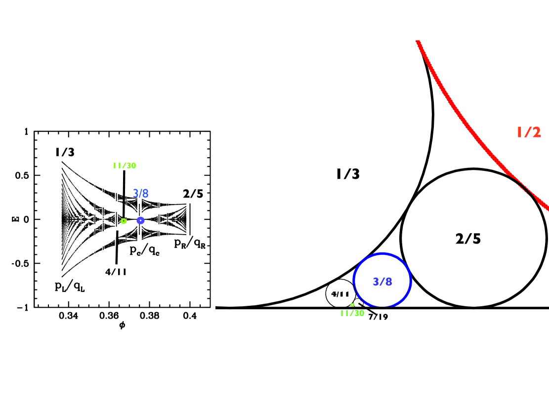
Figure 4: The left panel shows the first-generation butterfly (that resides inside the main butterfly) that stretches between $1/3$ and $2/5$, with its center (the blue pin) located at $3/8$. Inside it we see a next generation butterfly centered on $11/30$, and with left and right edges at $4/11$ and $7/19$. These ideas involving generations of central butterflies map elegantly onto isomorphic ideas involving Ford circles, which are shown in the right panel . Ford circles representing the butterfly centers for three successive generations are shown in red (main butterfly), blue, and green. The red arc is the part of the circle representing the main butterfly centered at $1/2$.

In the butterfly graph, there are three rational numbers that define, respectively, the left edge, the center and the right edge of a butterfly, and these three rationals form a Farey triplet $(\frac{p_{L}}{q_{L}},\frac{p_{c}}{q_{c}},\frac{p_{R}}{q_{R}})$ obeying the Farey sum condition: $\frac{p_{c}}{q_{c}}=\frac{p_{L}+p_{L}}{q_{L}+q_{R}}$. These three rationals can also be represented in terms of three mutually kissing Ford circles, sitting on a horizontal axis (a circle of infinite radius), and having curvatures $2q_{L}^{2},2q_{c}^{2},$ and $2q_{R}^{2}$.

Such a quadruple of (generalized) circles, will be referred as a “Ford–Apollonian”, meaning a set of four mutually kissing circles that have curvatures that make up a quadruple $(q_{c}^{2},q_{R}^{2},q_{L}^{2},0)$ , which we will denote as $(\kappa_{c},\kappa_{R},\kappa_{L},0)$. Here we have eliminated the common factor of $2$. The butterfly recursions ( see Eq. (7)) can be written as,

$$\sqrt{\kappa_{c}(l+1)}=4\sqrt{\kappa_{c}(l)}-\sqrt{\kappa_{c}(l-1)},\quad\zeta(l)=\sqrt{\frac{\kappa_{c}(l+1)}{\kappa_{c}(l)}}=4-\frac{1}{\zeta(l-1)}$$ (16)

$$(\zeta^{*})^{2}-4\zeta^{*}+1=0,\quad\zeta^{*}=\lim_{l\rightarrow\infty}\sqrt{\frac{\kappa_{c}(l+1)}{\kappa_{c}(l)}}\rightarrow 2+\sqrt{3}$$ (17)

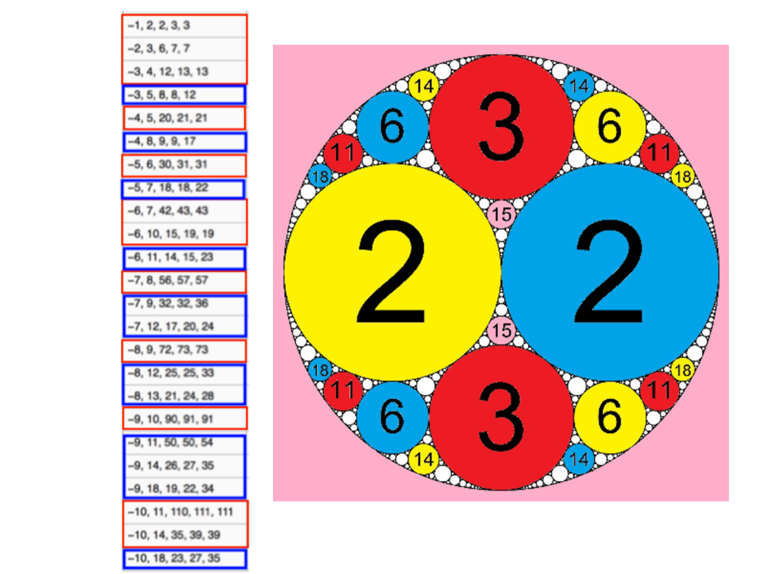
Figure 5: The table on the left lists the curvatures of some of the largest circles in the $\cal{IAG}$. Red frames represent configurations that are dual to Ford Apollonians while blue frame do not. Only the first three curvatures (of the five displayed in the table) are needed to completely describe each gasket . On the right is shown the gasket $(-1,2,2,3,3)$ and the infinite packing of circles inside. Every trio of mutually tangent circles has two other circles to which the three are tangent, and their curvatures satisfy Descartes configuration.

5.2 Integral Apollonian Gaskets – $\cal{IAG}$

An integral Apollonian gasket is an intricate hierarchical structure consisting of an infinite number of mutually kissing (i.e., tangent) circles that are nested inside each other, growing smaller and smaller at each level. At each hierarchical level there are sets of four circles that are all tangent, and associated with each such set of circles is a quadruplet of integers that are their curvatures (the reciprocals of their radii). The table in Figure 5 lists some examples. We note that unlike the Ford Apollonian which includes a straight line – that can be viewed as a circle of zero curvature - all members of an $\cal{IAG}$ are characterized by non-zero curvatures.

5.3 Descartes’s theorem

The geometry of four mutually tangent circles is described in terms of Descartes’s theorem. if four circles are tangent ( or kissing) to each other, and the circles have curvatures (inverse of the radius) $k_{i}$( $i=0,1,2,3$), a relation between the curvatures $k_{i}$ of these circles is given by,

$$(k_{0}+k_{1}+k_{2}+k_{3})^{2}=2(k_{0}^{2}+k_{1}^{2}+k_{2}^{2}+k_{3}^{2}).$$ (18)

Solving for $k_{0}$ in terms of $k_{i}$, $i=1,2,3$ gives,

$$k_{0}(\pm)=k_{1}+k_{2}+k_{3}\pm 2\delta,\,\ \delta=\sqrt{\kappa_{1}\kappa_{2}+\kappa_{2}\kappa_{3}+\kappa_{1}\kappa_{3}}$$ (19)

The two solutions $\pm$ respectively correspond to the inner and the outer bounding circles shown in left panel in Fig. 5. The consistent solutions of above set of equations require that bounding circle must have negative curvature. We note that

$$k_{0(+)}+k_{0(-)}=2(k_{1}+k_{2}+k_{3})$$ (20)

Important consequence of this linear equation is that if the first four circles in the gasket have integer curvatures, then every other circle in the packing does too. We note that Ford Apollonian representing the butterfly is a special case of an $\cal{IAG}$ with $\kappa_{3}=0$.

5.4 Duality

Interestingly, it turns out that Ford–Apollonian gaskets are related to $\cal{IAG}$ by a duality transformation — that is, an operation that is its own inverse (also called an “involution”). This transformation amounts to a bridge that connects the butterfly fractal, which is made up of Ford–Apollonian quadruples, with the world of $\cal{IAG}$s. We now proceed to describe this self-inverse transformation both geometrically and algebraically.

If we write the curvatures of four kissing circles as a vector $A$ with four integer components, we can use matrix multiplication to obtain another such 4-vector $\bar{A}$. In particular, consider the matrix $\hat{D}$:

$$\hat{D} = \frac{1}{2}\left(\begin{array}[]{cccc}-1&1&1&1\\ 1&-1&1&1\\ 1&1&-1&1\\ 1&1&1&-1\\ \end{array}\right),\,\,\bar{A}=\hat{D}A$$

The matrix $\hat{D}$ is its own inverse. As is shown above, if we multiply $A$ (the 4-vector of curvatures) by $\hat{D}$, we obtain its dual 4-vector $\bar{A}$. Since $\hat{D}^{2}=1$, this transformation maps the dual gasket back onto the original gasket. In terms of butterfly coordinates, the relationship between the Ford-Apollonian $(q_{c}^{2},q_{R}^{2},q_{L}^{2},0)\equiv(\kappa_{c},\kappa_{R},\kappa_{L},0)$ representing the butterfly and the corresponding $\cal{IAG}$ is given by the following equation.

$$(\kappa_{c},\kappa_{R},\kappa_{L},0)=\hat{D}(-\kappa_{0},\kappa_{1},\kappa_{2},\kappa_{3})=\hat{D}(-q_{L}q_{R},q_{c}q_{R},q_{c}q_{L},q_{L}q_{R}+q_{R}^{2}+q_{L}^{2})$$ (22)

It is easy to show that $\delta$ (see Eq. 19) is the curvature of the “dual circle”.

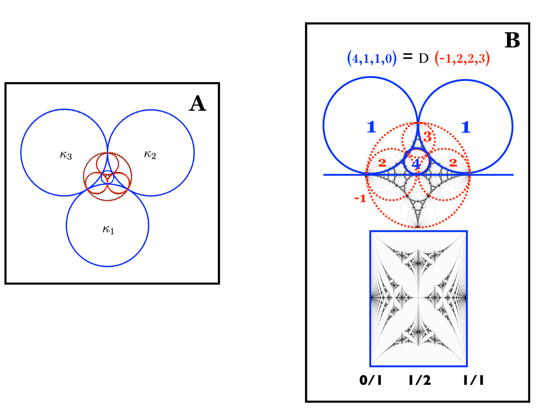
Figure 6: (A) An illustration of duality : four mutually tangent circles (red circles) and their dual image (blue circles). Each circle in the dual set passes through three of the kissing points of the original set of circles. (B) shows the correspondence between the $\cal{IAG}$ $(-1,2,2,3)$ (top) and the butterfly centered at flux-value $\phi=1/2$, and with edges at $0/1$ and $1/1$ (bottom). The blue circles are Ford circles, representing the butterfly’s center and edges, with reduced curvatures $(4,1,1)$, all tangent to the horizontal line (whose curvature is zero). These four circles with curvature 4-vector $(4,1,1,0)$ form a Ford–Apollonian gasket that is dual to the $(-1,2,2,3)$ $\cal{IAG}$, which is shown in red.

5.5 $\cal{ABC}$ and the Chern Numbers

We now address the following key question: Given four kissing circles making up an $\cal{IAG}$, along with their integer curvatures, what are the Chern numbers of the corresponding butterfly?

It turns out that $\delta$, the curvature of the “dual circle” –that is the circle passing through the tangency points of the three inner circles encodes the Chern numbers of the butterfly at least in the cases where the mathematical framework underlying $\cal{ABC}$ is well established. The Chern numbers for a butterfly centered at flux-value $\phi=\frac{p_{c}}{q_{c}}$ are:

$$\sigma_{\pm} \,\,=\,\,\, \pm\frac{\sqrt{\delta}}{2}\,\,=\,\,\pm\frac{1}{2}(\kappa_{1}\kappa_{2}+\kappa_{2}\kappa_{3}+\kappa_{1}\kappa_{3})^{1/4}\,\,=\,\,\pm\frac{q_{c}}{2}$$ (23)

5.6 Relation to $D_{3}$ symmetric Apollonian

We next show that the butterfly scaling ratio $R_{\phi}$ associated with the butterfly hierarchy as described above is related to the nested set of circles in an $\cal{IAG}$ with $D_{3}$ symmetry. We consider a special case where $\kappa_{1}=\kappa_{2}=\kappa_{3}=\kappa$ corresponding to an Apollonian gasket that has perfect $D_{3}$ symmetry. Using Eq. 19, the ratio of the curvatures of the inner and outer circles is determined by the equations:

$$\frac{\kappa_{0}(+)}{\kappa} = \sqrt{3}(2+\sqrt{3}),\quad\frac{\kappa_{0}(-)}{\kappa}=\sqrt{3}(2-\sqrt{3}),\,\,\ \frac{\kappa_{0}(+)}{\kappa_{0}(-)}=(2+\sqrt{3})^{2}$$ (24)

The irrational ratio of these two curvatures shows that there is no integral Apollonian gasket possessing exact $D_{3}$ symmetry. Interestingly, however, in some integral Apollonian gaskets, perfect $D_{3}$ symmetry is asymptotically approached as one descends deeper and deeper into the gasket, thus getting larger and larger integral values of the curvature, which give closer and closer rational approximations to the irrational limit, $(2+\sqrt{3})^{2}$.

The $D_{3}$ symmetry described above appears rather mysterious as it lacks any geometrical picture that may help in visualizing what this symmetry means for the butterfly landscape. Clearly, no butterfly in the entire butterfly graph exhibits this symmetry. The question of this hidden symmetry in the butterfly landscape is tied to kaleidoscopic properties as described below.

An Apollonian gasket is like a kaleidoscope in which the image of the first four circles is reflected again and again through an infinite collection of curved mirrors. In particular $\kappa_{0}(+)$ and $\kappa_{0}(-)$ are mirror images through a circular mirror passing though the tangency points of $\kappa_{1}$, $\kappa_{2}$ and $\kappa_{3}$. The curvature of this circular mirror is equal to $\delta$.

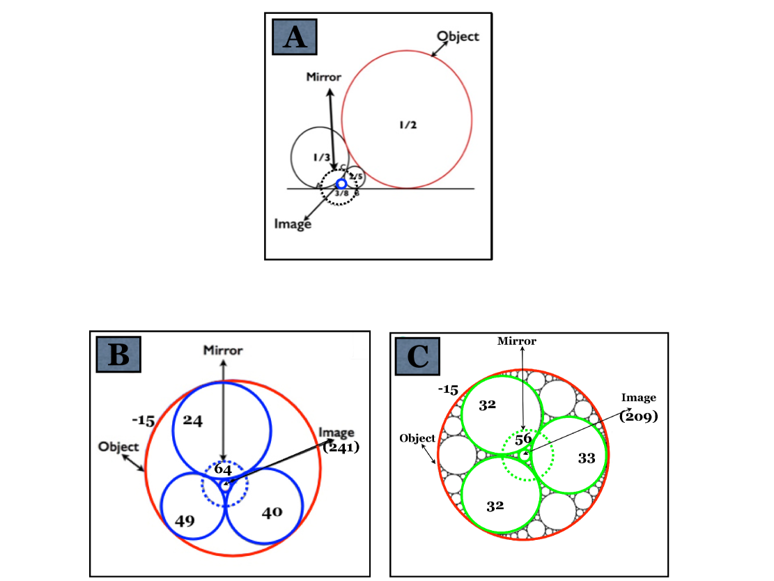
Figure 7: This figure illustrates the kaleidoscopic aspect of Apollonian gaskets where the outermost circle ( labeled object, shown in red) and the innermost circle (labeled image) are mirror images of each other, reflected through a (dotted) circle that passes through the tangency points of three other circles. A, B, C respectively show the kaleidoscopic aspects of the Ford Apollonian representing the butterfly centered at $3/8$, its dual $\cal{IAG}$ $(-15,24,40,49)$ (left) and its symmetric dual partner $(-15,32,32,33)$ (right).

Figure 8: A set of Apollonian gaskets having almost $D_{3}$ symmetry (as seen from the curvatures of circles labeled in red). The negative number and the number in the bracket respectively label the curvatures of the outer and the innermost circles which are mirror images through the dotted circles. The figure shows two sequences $(4,56,780...)$ (left) and $(15,209,2911...)$ ( right), showing three entries in each case where even and odd-curvatures separate into two distinct hierarchies (See Eq. 14). Lines with the arrows show the iterative process where the curvatures of the innermost circles form the next generation of Apollonians. Together, the sequence $(4,15,56,209,780,2911,...)$ , represents the Chern numbers associated with the butterfly hierarchy in the magnetic-flux interval $[1/3-2/5]$ that is shown in Fig. 2.

5.7 Butterfly Nesting and Kaleidoscope

In our discussion of the butterfly hierarchies, the kaleidoscopic aspect of the Ford Apollonian takes a special meaning as the object and the mirror represent two successive generations of a butterfly. In this case, the object and the mirror can be identified with the curvatures of the Ford circles representing two successive levels of the butterfly center, which we denote as as $\kappa^{b}_{-}$ and $\kappa^{b}_{+}$

$$\kappa^{b}_{+} = [\sqrt{\kappa_{L}}+\ \sqrt{\kappa_{R}}]^{2}\equiv\kappa_{c}(l),\,\,\quad\kappa^{b}_{-}=[\sqrt{\kappa_{L}}-\ \sqrt{\kappa_{R}}]^{2}\equiv\kappa_{c}(l-1)$$

Written in terms of butterfly coordinates, we obtain the following equation.

$$\frac{\kappa^{b}_{+}}{\kappa^{b}_{-}}=[\frac{1+q_{R}/q_{L}}{1-q_{R}/q_{L}}]^{2}$$ (25)

The corresponding ratio $\frac{k_{0}(+)}{\kappa_{0}(-)}$ for the $\cal{IAG}$, using Eq. (22) is given by,

$$\frac{k_{0}(+)}{\kappa_{0}(-)}=\frac{7q_{L}q_{R}+4q_{L}^{2}+4q_{L}^{2}}{q_{L}q_{R}}=7+\frac{q_{L}}{q_{R}}+\frac{q_{R}}{q_{L}}$$ (26)

For the butterfly hierarchy, $\frac{q_{R}}{q_{L}}\rightarrow\sqrt{3}$ ( see Eq. (13) ). Therefore, we get,

$$\frac{\kappa^{b}_{+}}{\kappa^{b}_{-}}=\frac{\kappa_{c}(l)}{\kappa_{c}(l-1)} \rightarrow 7+4\sqrt{3}=(2+\sqrt{3})^{2},\,\,\quad\frac{\kappa_{0(+)}}{\kappa_{0(-)}}\rightarrow 7+\frac{4}{\sqrt{3}}$$

Therefore, $\frac{\kappa^{b}_{+}}{\kappa^{b}_{-}}$ gives the correct scaling for the magnetic flux interval as given by Eq. (12).

Figure (7) illustrates the relationship between the butterfly, its dual $\cal{IAG}$ and the corresponding Apollonian that evolves into a $D_{3}$-symmetric configuration.

Given a butterfly represented by $(\kappa_{c},\kappa_{R},\kappa_{L},0)$ and its dual partner $(\kappa_{0},\kappa_{1},\kappa_{2},\kappa_{3})$ there exists another Apollonian that encodes the nesting characteristics of the butterfly. This “conjugate” Apollonian which we denote as $(-\kappa_{0}^{s},\kappa^{s}_{1},\kappa^{s}_{2},\kappa^{s}_{3})$ will be referred as the symmetric-dual Apollonian associated with the butterfly. For the butterfly hierarchy described here, it is found to be given by,

$$(-\kappa^{s}_{0},\kappa^{s}_{1},\kappa^{s}_{2},\kappa^{s}_{3}) = (-\kappa_{0},\frac{\kappa_{1}+\kappa_{2}}{2},\frac{\kappa_{1}+\kappa_{2}}{2},\frac{\kappa_{1}+\kappa_{2}}{2}+d)$$ (27)

$$= (-q_{L}q_{R},\frac{q_{c}^{2}}{2},\frac{q_{c}^{2}}{2},\frac{q_{c}^{2}}{2}+d)$$ (28)

where $d=\frac{3q_{L}^{2}-q_{R}^{2}}{2}$ reflects a deviation from the $D_{3}$ symmetry and is invariant ( independent of $l$ ) for a given “set of zooms” corresponding to various generations of the butterfly. Asymptotically, one recovers the $D_{3}$ symmetry as $d=\frac{3q_{L}^{2}}{2}-\frac{q_{R}^{2}}{2}\rightarrow 0$ as $\frac{q_{R}}{q_{L}}\rightarrow\sqrt{3}$. Fig. 8 shows a sequence of $\cal{IAG}$ that asymptotically evolve into $D_{3}$-symmetric configurations.

6 Conclusions and Open Challenges

In systems with competing length scales, the interplay of topology and self-similarity is a fascinating topic that continues to attract physicists as well as mathematicians. The butterfly graphs in Harper and its various generalizations SN ; GHarper ; ML encode beautiful and highly instructive physical and mathematical idea and the notion that they are related to abstract and popular fractals reflects the mystique, the beauty and simplicity of the laws of nature. The results described above point towards a very deep and beautiful link between the Hofstadter butterfly and the Apollonian gaskets. Among many other things, nature has indeed found a way to use beautiful symmetric Apollonian gaskets in the quantum mechanics of the two-dimensional electron gas problem. This paper addresses this fascinating topic that is still in its infancy.

As stated above, the dual of the Ford–Apollonian gaskets that map to butterfly configurations constitute only a subset of the entire set of $\cal{IAG}$ . It appears, however, that the butterfly graphs with a hierarchy of gaps can be mapped to non-Ford–Apollonian gaskets by regrouping some of those gaps that do not follow the Farey triplet rule. For further details, we refer readers to Ref. (kitab ) where readers will find examples of additional correspondences between the butterfly and the $\cal{IAG}$. We also note that the description of off-centered butterflies (miniature butterflies whose centers are not located at $E=0$ in the butterfly graph) in terms of Apollonians remains an open problem. Another intriguing question about whether Chern numbers describe some special geometric property of configurations of four kissing circles and whether Chern numbers have any topological mean for Apollonians remains elusive. A systematic mathematical framework that relates the butterfly to the set of $\cal{IAG}$ is an open problem. We believe that satisfactory answers to many subtle questions may perhaps be found within the mathematical framework of conformal and Möbius transformations.

References

- (1) Azbel’ M YaJETP, Vol. 19, No. 3, p. 634 (1964).
- (2) D. Langbein, Physical Review 180, 633 (1969).
- (3) D. Hofstadter, Phys Rev B, 14 (1976) 2239.
- (4) von Klitzing K, Dorda G and Pepper M , Phys. Rev. Lett 45 494 (1980).
- (5) Michael V. Berry, , Proceedings of the Royal Society A 392 (1984), 45; Barry Simon, , Physical Review Letters 51 (1983), 2167.
- (6) C. R Dean et al, Nature 12186, 2013; M. Aidelsburger, Phys Rev Lett, 111 185301 (2013); Hirokazu Miyake et al, Phys Rev Lett, 111 185302 (2013).
- (7) Wannier, G. H. , Phys. Status Solidi B 88, 757–765 (1978); F. H. Claro and G. H. Wannier, Phys Rev B, 19 (1979) 19.
- (8) MacDonald, A. Phys. Rev. B 28, 6713–6717 (1983).
- (9) M. Wilkinson, J. Phys. A: Math. Gen. 20 (1987)4337-4354; J. Phys. A: Math, Gen.21 (1994) 8123-8148.
- (10) Dana Mackenzie, American Scientist, Vol 98, Page 10 , (2010);
- (11) L. R. Ford, The American Mathematical Monthly, Vol 39, no 9, 1938, page 586.
- (12) The theorem is named after Rene Descartes, who stated it in 1643. See R. Descartes. Oeuvres de Descartes, Correspondence IV, (C. Adam and P. Tannery, Eds.), Paris: Leopold Cerf 1901.
- (13) ” Butterfly in the Quantum World, Story of a most fascinating quantum Fractal”, Indubala I Satija, IOP Concise Physics, in print, 2016.
- (14) I. Satija and G. Naumis, Phys Rev B 88 054204 (2013);Erhai Zhao, Noah Bray-Ali, C. Williams, Ian Spielman and Indubala I Satija , Phys Rev A, 84, 2011, 063629
- (15) A. Avila, S. Jitomikskaya and C. A. Marx arxiv. 1602.05111 ( unpublished).
- (16) M. Lababidi, I Satija and E. Zhao, Phys Rev Lett, 112 (2014) 026805.