Tetrahedral shapes of neutron-rich Zr isotopes from multidimensionally-constrained relativistic Hartree-Bogoliubov model

Abstract

We develop a multidimensionally constrained relativistic Hartree-Bogoliubov (MDC-RHB) model in which the pairing correlations are taken into account by making the Bogoliubov transformation. In this model, the nuclear shape is assumed to be invariant under the reversion of $x$ and $y$ axes; i.e., the intrinsic symmetry group is $V_{4}$ and all shape degrees of freedom $\beta_{\lambda\mu}$ with even $\mu$ are included self-consistently. The RHB equation is solved in an axially deformed harmonic oscillator basis. A separable pairing force of finite range is adopted in the MDC-RHB model. The potential energy curves of neutron-rich even-even Zr isotopes are calculated with relativistic functionals DD-PC1 and PC-PK1 and possible tetrahedral shapes in the ground and isomeric states are investigated. The ground state shape of ¹¹⁰Zr is predicted to be tetrahedral with both functionals and so is that of ¹¹²Zr with the functional DD-PC1. The tetrahedral ground states are caused by large energy gaps around $Z=40$ and $N=70$ when $\beta_{32}$ deformation is included. Although the inclusion of the $\beta_{30}$ deformation can also reduce the energy around $\beta_{20}=0$ and lead to minima with pear-like shapes for nuclei around ¹¹⁰Zr, these minima are unstable due to their shallowness.

I Introduction 

The intrinsic shape of most known nuclei deviates from a sphere Bohr and Mottelson (1969, 1975). The deformation of a nucleus can be described by the parametrization of the nuclear surface with a multipole expansion,

$$R(\theta,\varphi)=R_{0}\left[1+\beta_{00}+\sum_{\lambda=1}^{\infty}\sum_{\mu=-\lambda}^{\lambda}\beta_{\lambda\mu}^{*}Y_{\lambda\mu}(\theta,\varphi)\right],$$ (1)

where $\beta_{\lambda\mu}$’s are deformation parameters. Various nuclear deformations characterized by $\beta_{\lambda\mu}$ with different $\{\lambda,\mu\}$ are connected with many nuclear phenomena which have been predicted and some of them have also been observed.

In recent decades, the triaxiality and reflection asymmetry in nuclear shapes have become more and more attractive because several interesting theoretical predictions related to these shapes have been confirmed experimentally. The static triaxial shapes may result in the wobbling motion Bohr and Mottelson (1975) or chiral doublet bands Frauendorf and Meng (1997) in atomic nuclei; both phenomena were observed in 2001 Odegard et al. (2001); Starosta et al. (2001). In 2006, Meng et al. predicted that multiple chiral doublet (M$\chi$D) bands may exist in one nucleus with different triaxial configurations Meng et al. (2006a). In recent years, M$\chi$D bands were indeed found in several nuclei Ayangeakaa et al. (2013); Lieder et al. (2014); Kuti et al. (2014); Tonev et al. (2014); Liu et al. (2016). The triaxiality may also play a role in the low-spin signature inversion Bengtsson et al. (1984); Liu et al. (1995, 1996); Zhou et al. (1996); Riedinger et al. (1997); Liu et al. (1998). Moreover, the development of triaxial shapes could lead to the termination of rotational bands in nuclei with $A\simeq 110$; see Ref. Afanasjev et al. (1999) for a review. The pear-like nuclear shape, characterized by $\beta_{30}$, was predicted to be very pronounced in many nuclei Butler and Nazarewicz (1996); Möller et al. (2008); Agbemava et al. (2016). Low-lying negative-parity levels which are connected with the ground state band via strong $E1$ transitions in actinides and some rare-earth nuclei are related to reflection asymmetric shapes with nonzero $\beta_{30}$ Shneidman et al. (2003, 2006); Wang et al. (2005); Yang et al. (2009); Robledo and Bertsch (2011); Zhu et al. (2012a, b); Nomura et al. (2013, 2014, 2015). The direct evidence for a static octupole deformation has been shown experimentally in ²²⁴Ra Gaffney et al. (2013) and in ${}^{144}\mathrm{Ba}$ Bucher et al. (2016).

What new features can we expect if the nonaxial and reflection asymmetric deformations are put together or combined? It has been revealed in Ref. Lu et al. (2012a) that both the triaxial and octupole shapes become important around the second saddle point in the potential energy surface (PES) of actinide nuclei and they lower the second fission barrier considerably. Recently, Liu et al. observed for the first time octupole correlations between M$\chi$D bands in ⁷⁸Br and proposed that chirality-parity quartet bands may appear in a nucleus with both a static triaxial deformation ($\beta_{22}$) and an octupole deformation ($\beta_{30}$) Liu et al. (2016).

The nonaxiality and reflection asymmetry are combined intrinsically in deformations characterized by $\beta_{\lambda\mu}$ with odd $\lambda$ and nonzero $\mu$. Among such deformations, the $\beta_{32}$ deformation is of particular interest and has been investigated extensively Hamamoto et al. (1991); Skalski (1991); Li and Dudek (1994); Takami et al. (1998); Yamagami et al. (2001); Dudek et al. (2002, 2006); Olbratowski et al. (2006); Zberecki et al. (2006); Dudek et al. (2010). A nucleus with a pure $\beta_{32}$ deformation, i.e., $\beta_{\lambda\mu}=0$ if $\lambda\neq 3$ and $\mu\neq 2$, has a tetrahedral shape with the symmetry group $T_{d}^{D}$. The study of single-particle structure of a nucleus with tetrahedral symmetry predicted large energy gaps at $Z(N)=16$, 20, 32, 40, 56–58, 70, and 90–94 and $N=112$ and 136/142 Li and Dudek (1994); Dudek et al. (2002, 2007, 2003); Heiss et al. (1999); Arita and Mukumoto (2014). These shell gaps are comparable to or even stronger than those at spherical shapes. Thus, a nucleus with proton and/or neutron numbers equal to these values may have a static tetrahedral shape or strong tetrahedral correlations.

Various nuclei such as ^80,108,110Zr, ¹⁶⁰Yb, ¹⁵⁶Gd, and ²⁴²Fm were predicted to have ground or isomeric states with tetrahedral shapes from the macroscopic-microscopic (MM) model Dudek et al. (2002, 2007, 2006); Schunck et al. (2004); Dudek et al. (2014) and the Skyrme Hartree-Fock (SHF) model, the SHF plus BCS model, or the Skyrme Hartree-Fock-Bogoliubov (SHFB) model Dudek et al. (2007); Schunck et al. (2004); Dudek et al. (2006); Yamagami et al. (2001); Olbratowski et al. (2006); Zberecki et al. (2009, 2006); Takami et al. (1998). The possible existence of tetrahedral symmetry in light nuclei such as ¹⁶O Bijker and Iachello (2014) as well as superheavy nuclei Chen and Gao (2013, 2010) was also proposed. Furthermore, the rotational properties of tetrahedral nuclei have been studied theoretically Gao et al. (2004); Tagami et al. (2013, 2015) which would certainly be helpful for experimentalists to identify tetrahedral nuclei.

Several experiments were devoted to the study of tetrahedral shapes in ¹⁶⁰Yb Bark et al. (2010), ^154,156Gd Bark et al. (2010); Jentschel et al. (2010); Doan et al. (2010), ^230,232U Ntshangase et al. (2010), and ¹⁰⁸Zr Sumikama et al. (2011). For ¹⁶⁰Yb and ^154,156Gd, although the observed odd and even-spin members of the lowest energy negative-parity bands are similar to the proposed tetrahedral band of ¹⁵⁶Gd, the deduced nonzero quadrupole moments existence of tetrahedral shapes in these nuclei. The possibility of a tetrahedral shape for the negative-parity bands in ^230,232U was excluded in Ref. Ntshangase et al. (2010) by the observed similarity in the energies and electric dipole moments of those bands in the $N=138$ and $N=140$ isotones and the measured values for quadrupole moment $Q_{2}$ in ²²⁶Ra. An isomeric state observed in ¹⁰⁸Zr has been assigned a tetrahedral shape Sumikama et al. (2011). However, this isomeric state can also been explained by assuming an axial shape with the angular momentum projected shell model Liu et al. (2011, 2015).

Besides the tetrahedral shape which corresponds to a pure $\beta_{32}$ deformation, the study of nuclear shapes with a non-zero $\beta_{32}$ superposed on a sizable $\beta_{20}$ has become a hot topic too. In recent years, nuclei with $Z\simeq 100$ have been studied extensively because such studies can not only reveal the structure for these nuclei but also give useful structure information for superheavy nuclei Afanasjev et al. (2003); Leino and Hessberger (2004); Herzberg et al. (2006); Herzberg and Greenlees (2008); Zhang et al. (2011, 2012, 2013); Liu et al. (2014); Shi et al. (2014); Wang et al. (2014); Afanasjev (2014); Agbemava et al. (2015); Afanasjev (2015); Li and He (2016). One example of such studies is the observation of very low-lying $2^{-}$ bands in several even-$Z$ $N=150$ isotones Robinson et al. (2008). This low-lying feature was argued by Chen et al. to be a fingerprint of sizable $\beta_{32}$ in these well deformed nuclei Chen et al. (2008). A self-consistent and microscopic study of $Y_{32}$ effects in these $N=150$ isotones was carried out in Ref. Zhao et al. (2012) and it was found that, for ground states of ²⁴⁸Cf and ²⁵⁰Fm, $\beta_{32}>0.03$ and the energy gain due to the $\beta_{32}$ distortion is more than 300 keV.

In this work we will study the potential energy surface and tetrahedral shape in neutron rich even-even Zr isotopes by using the covariant density function theory (CDFT). The nuclear CDFT is one of the state-of-the-art approaches for the study of ground states as well as excited states in nuclei ranging from light to superheavy regions Serot and Walecka (1986); Reinhard (1989); Ring (1996); Bender et al. (2003); Vretenar et al. (2005); Meng et al. (2006b); Paar et al. (2007); Nikšić et al. (2011); Liang et al. (2015); Meng and Zhou (2015); Meng (2016). Recently, the global performance of various relativistic functionals on the ground state properties and beyond-mean-field correlations of nuclei across the nuclear chart has also been examined Afanasjev et al. (2013); Agbemava et al. (2014); Lu et al. (2015); Agbemava et al. (2015); Afanasjev and Agbemava (2016).

Recently, we have developed multidimensionally constrained CDFT (MDC-CDFT) by breaking the reflection and axial symmetries simultaneously. In the MDC-CDFT, the nuclear shape is assumed to be invariant under the reversion of $x$ and $y$ axes; i.e., the intrinsic symmetry group is $V_{4}$ and all shape degrees of freedom $\beta_{\lambda\mu}$ with even $\mu$ ($\beta_{20}$, $\beta_{22}$, $\beta_{30}$, $\beta_{32}$, $\beta_{40}$, $\cdots$) are included self-consistently. The MDC-CDFT consists of two types of models: the multidimensionally constrained relativistic mean field (MDC-RMF) model and the multidimensionally constrained relativistic Hartree-Bogoliubov (MDC-RHB) model. In the MDC-RMF model, the BCS approach has been implemented for the particle-particle (pp) channel. This model has been used to study potential energy surfaces and fission barriers of actinides Lu et al. (2012a, 2014a, 2014b, 2014c, b); Zhao et al. (2015a), the spontaneous fission of several fermium isotopes Zhao et al. (2016), the $Y_{32}$ correlations in $N=150$ isotones Zhao et al. (2012), and shapes of hypernuclei Lu et al. (2011, 2014d); see Refs. Li et al. (2014); Lu et al. (2016); Zhou (2016) for recent reviews. The Bogoliubov transformation generalizes the BCS quasi-particle concept and provides a unified description of particle-hole (ph) and pp correlations on a mean-field level. In the MDC-RHB model, pairing correlations are treated by making the Bogoliubov transformation and a separable pairing force of finite range Tian and Ma (2006); Tian et al. (2009a, b); Nikšić et al. (2008) is adopted. Due to its finite range nature, the dependence of the results on the pairing cutoff can be avoided. The MDC-RHB model has been used to study the spontaneous fission of fermium isotopes Zhao et al. (2015b).

The detailed formulas for the MDC-RMF model have been presented in Ref. Lu et al. (2014b) and some applications of this model were reviewed in Refs. Li et al. (2014); Lu et al. (2016); Zhou (2016). In this paper, we present the formulas of the MDC-RHB model and its application to the study of tetrahedral shapes of neutron-rich Zr isotopes. The paper is organized as follows. The formalism of the MDC-RHB model is given in Sec. II. In Sec. III we present the numerical details and the results on neutron-rich even-even Zr isotopes. A summary is given in Sec. IV. Some detailed formulas used in the MDC-RHB model are given in Appendices A and B.

II Formalism of the MDC-RHB Model

In the CDFT, a nucleus is treated as a system of nucleons interacting through exchanges of mesons and photons Serot and Walecka (1986); Reinhard (1989); Ring (1996); Bender et al. (2003); Vretenar et al. (2005); Meng et al. (2006b); Paar et al. (2007); Nikšić et al. (2011); Liang et al. (2015); Meng and Zhou (2015); Meng (2016). The effects of mesons are described either by mean fields or by point-like interactions between the nucleons Nikolaus et al. (1992); Burvenich et al. (2002). The nonlinear coupling terms Boguta and Bodmer (1977); Brockmann and Toki (1992); Sugahara and Toki (1994) or the density dependence of the coupling constants Fuchs et al. (1995); Nikšić et al. (2002) were introduced to give correct saturation properties of nuclear matter. Accordingly, there are four types of covariant density functionals: the meson exchange or point-coupling nucleon interactions combined with the nonlinear or density dependent couplings. All these four types of functionals have been implemented in the MDC-RHB model. In this section, we mainly present the formalism of the RHB model with density dependent point couplings.

The starting point of the RHB model with density dependent point couplings is the following Lagrangian,

$$\mathcal{L}= \bar{\psi}(i\gamma_{\mu}\partial^{\mu}-M)\psi$$ (2)

$$-{1\over 2}\alpha_{S}({\rho})\rho_{S}^{2}-{1\over 2}\alpha_{V}({\rho})j_{V}^{2}-{1\over 2}\alpha_{TV}({\rho})\vec{j}_{TV}^{2}$$

$$-{1\over 2}\delta_{S}(\partial_{\nu}\rho_{S})(\partial^{\nu}\rho_{S})$$

$$-e{1-\tau_{3}\over 2}A_{\mu}j_{V}^{\mu}-{1\over 4}F^{\mu\nu}F_{\mu\nu},$$

where $M$ is the nucleon mass, $\alpha_{S}({\rho})$, $\alpha_{V}({\rho})$, and $\alpha_{TV}({\rho})$ are density-dependent couplings for different channels, $\delta_{S}$ is the coupling constant of the derivative term, and $e$ is the electric charge. $\rho_{S}$, $j_{V}$, and $\vec{j}_{TV}$ are the isoscalar density, isoscalar current, and isovector current, respectively.

With the Green’s function technique, one can derive the Dirac-Hartree-Bogoliubov equation Kucharek and Ring (1991); Ring (1996),

$$\int d^{3}\bm{r}^{\prime}\left(\begin{array}[]{cc}h-\lambda&\Delta\\ -\Delta^{*}&-h+\lambda\end{array}\right)\left(\begin{array}[]{c}U_{k}\\ V_{k}\end{array}\right)=E_{k}\left(\begin{array}[]{c}U_{k}\\ V_{k}\end{array}\right),$$ (3)

where $E_{k}$ is the quasiparticle energy, $\lambda$ is the chemical potential, and $\hat{h}$ is the single-particle Hamiltonian,

$$\hat{h}=\bm{\alpha}\cdot[\bm{p}-\bm{V}(\bm{r})]+\beta[M+S(\bm{r})]+V_{0}(\bm{r})+\Sigma_{R}(\bm{r}),$$ (4)

with the scalar potential, vector potential, and rearrangement terms,

$$S = \alpha_{S}(\rho)\rho_{S}+\delta_{S}\triangle\rho_{S},$$

$$V^{\mu} = \alpha_{V}(\rho)j_{V}^{\mu}+\alpha_{TV}(\rho)j_{TV}^{\mu}\cdot\vec{\tau}+e{1-\tau_{3}\over 2}A^{\mu},$$

$$\Sigma_{R} = {1\over 2}{\partial\alpha_{S}\over\partial\rho}\rho_{S}^{2}+{1\over 2}{\partial\alpha_{V}\over\partial\rho}j_{V}^{2}+{1\over 2}{\partial\alpha_{TV}\over\partial\rho}\vec{j}_{TV}^{2}.$$ (5)

As usual we assume that the states are invariant under the time-reversal operation, which means that, in the above equations, all the currents or time-odd components vanish. In this case the single-particle Hamiltonian (4) has the time-reversal symmetry. For convenience two vector densities are defined as the time-like components of the 4-currents $j_{V}$ and $j_{TV}$,

$$\rho_{V}(\bm{r})=j_{v}^{0}(\bm{r}),\qquad\rho_{TV}(\bm{r})=j_{TV}^{0}(\bm{r}),$$ (6)

which are the only surviving components. The densities are related to $U_{k}$’s and $V_{k}$’s through

$$\rho_{S}(\bm{r}) = \sum_{k>0}V_{k}^{\dagger}(\bm{r})\gamma_{0}V_{k}(\bm{r}),$$

$$\rho_{V}(\bm{r}) = \sum_{k>0}V_{k}^{\dagger}(\bm{r})V_{k}(\bm{r}),$$

$$\rho_{TV}(\bm{r}) = \sum_{k>0}V_{k}^{\dagger}(\bm{r})\tau_{3}V_{k}(\bm{r}).$$ (7)

In the above summations, the no-sea approximation is applied.

The pairing potential reads

$$\Delta_{p_{1}p_{2}}(\bm{r}_{1}\sigma_{1},\bm{r}_{2}\sigma_{2})= \int d^{3}\bm{r}_{1}^{\prime}d^{3}\bm{r}_{2}^{\prime}\sum_{\sigma_{1}^{\prime}\sigma_{2}^{\prime}}^{p_{1}^{\prime}p_{2}^{\prime}}$$ (8)

$$V_{p_{1}p_{2},p_{1}^{\prime}p_{2}^{\prime}}^{{\rm pp}}(\bm{r}_{1}\sigma_{1},\bm{r}_{2}\sigma_{2},\bm{r}_{1}^{\prime}\sigma_{1}^{\prime},\bm{r}_{2}^{\prime}\sigma_{2}^{\prime})$$

$$\times\kappa_{p_{1}^{\prime}p_{2}^{\prime}}(\bm{r}_{1}^{\prime}\sigma_{1}^{\prime},\bm{r}_{2}^{\prime}\sigma_{2}^{\prime}),$$

where $p=f,g$ is used to represent the large and small components of the Dirac spinor. $V^{{\rm pp}}$ is the effective pairing interaction and $\kappa(\bm{r}_{1}\sigma_{1},\bm{r}_{2}\sigma_{2})$ is the pairing tensor,

$$\kappa_{\alpha\alpha^{\prime}}(\bm{r_{1}}\sigma_{1},\bm{r_{2}}\sigma_{2})=\sum_{k>0}V^{*}_{\alpha k}(\bm{r_{1}}\sigma_{1})U_{\alpha^{\prime}k}(\bm{r_{2}}\sigma_{2}).$$ (9)

As is usually done in the RHB theory, only the large components of the spinors are used to build the pairing potential Serra and Ring (2002). In practical calculations this means

$$\Delta_{ff}(\bm{r}_{1}\sigma_{1},\bm{r}_{2}\sigma_{2})= \int d^{3}\bm{r}_{1}^{\prime}d^{3}\bm{r}_{2}^{\prime}\sum_{\sigma_{1}^{\prime}\sigma_{2}^{\prime}}$$ (10)

$$V_{ff,ff}^{{\rm pp}}(\bm{r}_{1}\sigma_{1},\bm{r}_{2}\sigma_{2},\bm{r}_{1}^{\prime}\sigma_{1}^{\prime},\bm{r}_{2}^{\prime}\sigma_{2}^{\prime})$$

$$\times\kappa_{ff}(\bm{r}_{1}^{\prime}\sigma_{1}^{\prime},\bm{r}_{2}^{\prime}\sigma_{2}^{\prime}).$$

The other components $\Delta_{fg}$, $\Delta_{gf}$, and $\Delta_{gg}$ are omitted.

In the pp channel, we use a separable pairing force of finite range Tian and Ma (2006); Tian et al. (2009a, b); Nikšić et al. (2008),

$$V(\bm{r}_{1}\sigma_{1},\bm{r}_{2}\sigma_{2},\bm{r}_{1}^{\prime}\sigma_{1}^{\prime},\bm{r}_{2}^{\prime}\sigma_{2}^{\prime}) = -G\delta(\bm{R}-\bm{R}^{\prime})P(r)P(r^{\prime})$$ (11)

$$\times\frac{1}{2}(1-P_{\sigma}),$$

where $G$ is the pairing strength and $\bm{R}=(\bm{r}_{1}+\bm{r}_{2})/2$ and $\bm{r}=\bm{r}_{1}-\bm{r}_{2}$ are the center-of-mass and relative coordinates, respectively. $P(\bm{r})$ denotes the Gaussian function,

$$P(\bm{r})={(4\pi a^{2})^{-3/2}}e^{-{r^{2}}/{4a^{2}}},$$ (12)

where $a$ is the effective range of the pairing force. The two parameters $G=G_{0}=728$ MeV$\cdot$fm³ and $a=0.644$ fm Tian et al. (2009a, b) have been adjusted to reproduce the density dependence of the pairing gap of symmetric nuclear matter at the Fermi surface calculated with the Gogny force D1S. In the present work, the pairing strength $G$ is fine-tuned to reproduce the pairing gaps of Zr isotopes as discussed in Sec. III.1.

The RHB equation (3) is solved by expanding the large and small components of the spinors $U_{k}(\bm{r}\sigma)$ and $V_{k}(\bm{r}\sigma)$ in an axially deformed harmonic oscillator (ADHO) basis Gambhir et al. (1990),

$$U_{k}(\bm{r}\sigma)= \left(\begin{array}[]{c}\sum_{\alpha}f_{U}^{k\alpha}\Phi_{\alpha}(\bm{r}\sigma)\\ \sum_{\alpha}g_{U}^{k\alpha}\Phi_{\alpha}(\bm{r}\sigma)\end{array}\right),$$ (13)

$$V_{k}(\bm{r}\sigma)= \left(\begin{array}[]{c}\sum_{\alpha}f_{V}^{k\alpha}\Phi_{\alpha}(\bm{r}\sigma)\\ \sum_{\alpha}g_{V}^{k\alpha}\Phi_{\alpha}(\bm{r}\sigma)\end{array}\right),$$

with

$$\Phi_{\alpha}(\bm{r}\sigma) = C_{\alpha}\phi_{n_{z}}(z)\phi_{n_{r}}^{m_{l}}(\rho)\frac{1}{\sqrt{2\pi}}e^{im_{l}\varphi}\chi_{m_{s}}(\sigma),$$ (14)

which are eigensolutions of the Schrödinger equation with an ADHO potential,

$$\left[-\frac{\hbar^{2}}{2M}\nabla^{2}+V_{B}(\rho,z)\right]\Phi_{\alpha}(\bm{r}\sigma)=E_{\alpha}\Phi_{\alpha}(\bm{r}\sigma),$$ (15)

with

$$V_{B}(\rho,z)=\frac{1}{2}M(\omega_{\rho}^{2}\rho^{2}+\omega_{z}^{2}z^{2}).$$ (16)

In Eq. (14), $C_{\alpha}$ is a constant introduced for convenience, $\alpha=\{n_{z},n_{r},m_{l},m_{s}\}$ is the collection of quantum numbers, and $\omega_{z}$ and $\omega_{\rho}$ are the oscillator frequencies along and perpendicular to the symmetry ($z$) axis, respectively. The deformation of the basis $\beta_{{\rm B}}$ is defined through relations $\omega_{z}=\omega_{0}\exp(-\sqrt{5/4\pi}\beta_{{\rm B}})$ and $\omega_{\rho}=\omega_{0}\exp(\sqrt{5/16\pi}\beta_{{\rm B}})$, where $\omega_{0}=(\omega_{z}\omega_{\rho}^{2})^{1/3}$ is the frequency of the corresponding spherical oscillator. These bases are also eigenfunctions of the $z$ component of the angular momentum $j_{z}$ with eigenvalues $K_{\alpha}=m_{l}+m_{s}$. For such a basis state $\Phi_{\alpha}(\bm{r}\sigma)$ we can define a time-reversal state by $\Phi_{\bar{\alpha}}(\bm{r}\sigma)=\mathcal{T}\Phi_{\alpha}(\bm{r}\sigma)$, where $\mathcal{T}=i\sigma_{y}K$ is the time-reversal operator and $K$ is the complex conjugation. It is easy to see that $\Phi_{\bar{\alpha}}(\bm{r}\sigma)$ is also an eigensolution of Eq. (15) with the same energy $E_{\alpha}$, while the direction of the angular momentum is reversed, $K_{\bar{\alpha}}=-K_{\alpha}$. $\{\Phi_{\alpha},\Phi_{\bar{\alpha}}|K_{\alpha}>0\}$ forms a complete and discrete basis set in the space of two-component spinors.

In practical calculations, the ADHO basis is truncated as Warda et al. (2002); Lu et al. (2014b),

$$\left[n_{z}/Q_{z}+(2n_{\rho}+|m|)/Q_{\rho}\right]\leq N_{f},$$ (17)

for the large component of the Dirac spinor. $N_{f}$ is a certain integer constant and $Q_{z}=\max(1,b_{z}/b_{0})$ and $Q_{\rho}=\max(1,b_{\rho}/b_{0})$ are constants calculated from the oscillator lengths $b_{0}=1/\sqrt{M\omega_{0}}$, $b_{z}=1/\sqrt{M\omega_{z}}$, and $b_{\rho}=1/\sqrt{M\omega_{\rho}}$. For the small component, the truncation is made up to $N_{g}=N_{f}+1$ major shells in order to avoid spurious states Gambhir et al. (1990). The convergence of the results on $N_{f}$ is discussed in Sec. III.1.

The $V_{4}$ symmetry is imposed in the MDC-CDFT Zhou (2016); i.e., the nuclear potentials and densities are invariant under the following operations

$$\hat{S}_{x}\phi(x,y,z)= \ \phi(-x,y,z),$$ (18)

$$\hat{S}_{y}\phi(x,y,z)= \ \phi(x,-y,z),$$

$$\hat{S}\phi(x,y,z)= \ \phi(-x,-y,z),$$

where $\phi(x,y,z)$ represents nuclear potentials and densities. Thus, both axial symmetry and reflection symmetry are broken. Due to the $V_{4}$ symmetry, one can introduce a simplex operator $\hat{S}=ie^{-i\pi j_{z}}$ to block-diagonalize the RHB matrix. For a fermionic system, $\hat{S}$ is a Hermitian operator and satisfies $\hat{S}^{2}=1$. The basis states are also eigenstates of $\hat{S}$ with $\hat{S}\Phi_{\alpha}=(-1)^{K_{\alpha}-\frac{1}{2}}\Phi_{\alpha}$, which means that $\Phi_{\alpha}$ with $K_{\alpha}=\frac{1}{2},-\frac{3}{2},\frac{5}{2},-\frac{7}{2},\cdots$ span a subspace with $S=+1$, while their time-reversal states span the one with $S=-1$. Due to the time-reversal symmetry, the RHB matrix is block-diagonalized into two smaller ones denoted by the quantum number $S=\pm 1$, respectively. Furthermore, for a system with the time-reversal symmetry, it is only necessary to diagonalize the matrix with $S=+1$ and the other half is obtained by making the time reversal operation on Dirac spinors.

In the $S=+1$ subspace, solving the RHB equation (3) is equivalent to diagonalizing the matrix

$$\left(\begin{array}[]{cc}\mathcal{A}-\lambda&\mathcal{B}\\ \mathcal{B}^{\dagger}&-\mathcal{A}^{*}+\lambda\end{array}\right)\left(\begin{array}[]{c}\mathcal{U}_{k}\\ \mathcal{V}_{k}\end{array}\right) = E_{k}\left(\begin{array}[]{c}\mathcal{U}_{k}\\ \mathcal{V}_{k}\end{array}\right),$$ (25)

where $\mathcal{U}_{k}=(\mathcal{U}_{k,\alpha})$ and $\mathcal{V}_{k}=(\mathcal{V}_{k,\bar{\alpha}})$ are column matrices, and

$$\mathcal{A}_{\alpha\alpha^{\prime}}=\langle\alpha|h|\alpha^{\prime}\rangle,\qquad\mathcal{B}_{\alpha\bar{\alpha^{\prime}}}=\langle\alpha|\Delta|\bar{\alpha^{\prime}}\rangle,$$ (26)

are matrix elements of the single-particle Hamiltonian and the pairing field, where $\alpha$ and $\alpha^{\prime}$ run over all the quantum numbers $\left\{n_{z},n_{r},m_{l},m_{s},p\right\}$ satisfying the truncation condition (17).

We expand the potentials $V(\bm{r})$ and $S(\bm{r})$ and the densities in Eq. (II) in terms of the Fourier series,

$$f(\rho,\varphi,z)=\sum_{\mu=-\infty}^{\infty}f_{\mu}(\rho,z)\frac{1}{\sqrt{2\pi}}\exp(i\mu\varphi).$$ (27)

By applying the symmetry conditions (18), it is easy to see that $f_{\mu}=f_{\mu}^{*}=f_{\bar{\mu}}$ and $V_{n}=0$ for odd $n$. Thus the expansion in Eq. (27) can be simplified as

$$f(\rho,\varphi,z)=f_{0}(\rho,z)\frac{1}{\sqrt{2\pi}}+\sum_{n=1}^{\infty}f_{n}(\rho,z)\frac{1}{\sqrt{\pi}}\cos(2n\varphi),$$ (28)

where

$$f_{0}(\rho_{,}z) = \frac{1}{\sqrt{2\pi}}\int_{0}^{2\pi}d\varphi f(\rho,\varphi,z),$$

$$f_{n}(\rho,z) = \frac{1}{\sqrt{\pi}}\int_{0}^{2\pi}d\varphi f(\rho,\varphi,z)\cos(2n\varphi),$$ (29)

are real functions of $\rho$ and $z$. The calculation of matrix elements $\mathcal{A}_{\alpha\alpha^{\prime}}$ and densities are similar to that of the MDC-RMF model; the details can be found in Appendices of Ref. Lu et al. (2014b).

Due to the finite range nature of the paring force given in Eq. (11), it is not easy to calculate the matrix element $V_{12,1^{\prime}2^{\prime}}^{{\rm pp}}$, where the numbers $1,2,1^{\prime}$, and $2^{\prime}$ denote the ADHO basis wave functions. In Ref. Tian et al. (2009b), the authors have shown that the anti-symmetrized matrix element $\bar{V}_{12,1^{\prime}2^{\prime}}^{{\rm pp}}=V_{12,1^{\prime}2^{\prime}}^{{\rm pp}}-V_{12,2^{\prime}1^{\prime}}^{{\rm pp}}$ can be written as a sum of separable terms in both axially deformed and anisotropic HO bases. For this purpose the first step is to represent the product of two single-particle HO wave functions as a sum of HO wave functions in their center-of-mass frame,

$$|n_{r_{1}}m_{1}\rangle|n_{r_{2}}m_{2}\rangle = \sum_{N_{p}M_{p}}\sum_{n_{p}m_{p}}M_{N_{p}M_{p}n_{p}m_{p}}^{n_{r_{1}}m_{1}n_{r_{2}}m_{2}}|N_{p}M_{p}\rangle|n_{p}m_{p}\rangle,$$

$$|n_{z_{1}}\rangle|n_{z_{2}}\rangle = \sum_{N_{z}n_{z}}M_{N_{z}n_{z}}^{n_{z_{1}}n_{z_{2}}}|N_{z}\rangle|n_{z}\rangle,$$ (30)

where $M_{N_{z}n_{z}}^{n_{z_{1}}n_{z_{2}}}$ and $M_{N_{p}M_{p}n_{p}m_{p}}^{n_{r_{1}}m_{1}n_{r_{2}}m_{2}}$ are the Talmi-Moshinski brackets which are given in Appendix B. The matrix element in the center-of-mass frame reads

$$V_{12,1^{\prime}2^{\prime}} = -2\sqrt{2}G\sum_{N_{z}N_{p}M_{p}}\left(W_{12}^{N_{z}N_{p}M_{p}}\right)^{*}W_{1^{\prime}2^{\prime}}^{N_{z}N_{p}M_{p}},$$ (31)

where

$$W_{12}^{N_{z}N_{p}M_{p}} = \delta_{K_{1}+K_{2},M_{p}}\delta_{\pi_{1}\pi_{2},(-1)^{N_{z}+|M_{p}|}}\tau_{1}\frac{1}{\sqrt{2}}C_{1}C_{2}$$ (32)

$$\times\left(\sum_{n_{z}}M_{N_{z}n_{z}}^{n_{z_{1}}n_{z_{2}}}V_{n_{z}}\right)$$

$$\times\left(\sum_{n_{p}}M_{N_{p}M_{p}n_{p}0}^{n_{r_{1}}m_{1}n_{r_{2}}m_{2}}U_{n_{p}}\right),$$

and

$$V_{n_{z}} = \frac{1}{(4\pi a^{2})^{1/2}}\int_{-\infty}^{\infty}dze^{-\frac{z^{2}}{2a^{2}}}\phi_{n_{z}}\left(z\right),$$

$$U_{n_{p}} = \frac{\sqrt{2\pi}}{4\pi a^{2}}\int_{0}^{\infty}d\rho\rho e^{-\frac{\rho^{2}}{2a^{2}}}R_{n_{p}}^{0}\left(\rho\right).$$ (33)

More details are given in Appendix A. The pairing field and pairing energy can also be written in the separable form as

$$\Delta_{12} = \sum_{1^{\prime}2^{\prime}}V_{12,1^{\prime}2^{\prime}}\kappa_{1^{\prime}2^{\prime}}$$ (34)

$$= -2\sqrt{2}G\sum_{N_{z}}\sum_{N_{p}M_{p}}\left(W_{12}^{N_{z}N_{p}M_{p}}\right)^{*}P^{N_{z}N_{p}M_{p}},$$

$$E_{{\rm pair}} = \frac{1}{2}\sum_{12,1^{\prime}2^{\prime}}V_{12,1^{\prime}2^{\prime}}\kappa_{12}^{*}\kappa_{1^{\prime}2^{\prime}}$$ (35)

$$= -\sqrt{2}G\sum_{N_{z}}\sum_{N_{p}M_{p}}|P^{N_{z}N_{p}M_{p}}|^{2},$$

where

$$P^{N_{z}N_{p}M_{p}}=\sum_{12}W_{12}^{N_{z}N_{p}M_{p}}\kappa_{12}.$$ (36)

Since $\hat{S}=ie^{-i\pi j_{z}}$ is conserved, we can check that the matrix element of the pairing tensor has the structure $\kappa_{12}=\delta_{S_{1},\bar{S_{2}}}\kappa_{12}$. Combined with the $\delta_{K_{1}+K_{2},M_{p}}$ in $W_{12}^{N_{z}N_{p}M_{p}}$, one gets

$$P^{N_{z}N_{p}M_{p}} = \sum_{12}\delta_{S_{1},\bar{S_{2}}}\delta_{K_{1}+K_{2},M_{p}}W_{12}^{N_{z}N_{p}M_{p}}\kappa_{12}$$ (37)

$$= \delta_{M_{p},2n}P^{N_{z}N_{p}M_{p}},\quad n\in Z,$$

i.e., only $P^{N_{z}N_{p}M_{p}}$ with even $M_{p}$ survive and thus we can skip safely those with odd $M_{p}$ in the sum in Eq. (34). The sum in Eq. (31) runs over the ADHO quantum numbers $N_{z}$, $N_{p}$, and $M_{p}$ in the center-of-mass frame with $N_{z}+2N_{p}+|M_{p}|\leq 2N_{f}$.

The total energy of the nucleus reads

$$E_{{\rm total}} = \int d^{3}\bm{r}\left\{\sum_{k}v_{k}^{2}\psi_{k}^{\dagger}\left(\bm{\alpha}\cdot\bm{p}+\beta M_{{\rm B}}\right)\psi_{k}\right.$$ (38)

$$+\ \frac{1}{2}\alpha_{S}\rho_{S}^{2}+\frac{1}{2}\alpha_{V}\rho_{V}^{2}+\frac{1}{2}\alpha_{TS}\rho_{TS}^{2}+\frac{1}{2}\alpha_{TV}\rho_{TV}^{2}$$

$$+\ \frac{1}{3}\beta_{S}\rho_{S}^{3}+\frac{1}{4}\gamma_{S}\rho_{S}^{4}+\frac{1}{4}\gamma_{V}\rho_{V}^{4}$$

$$+\ \frac{1}{2}\delta_{S}\rho_{S}\Delta\rho_{S}+\frac{1}{2}\delta_{V}\rho_{V}\Delta\rho_{V}$$

$$\left.+\ \frac{1}{2}\delta_{TS}\rho_{TS}\Delta\rho_{TS}+\frac{1}{2}\delta_{TV}\rho_{TV}\Delta\rho_{TV}+\frac{1}{2}e\rho_{C}A\right\}$$

$$+\ E_{{\rm pair}}+E_{{\rm c.m.}},$$

where the center-of-mass correction $E_{{\rm c.m.}}$ is calculated, depending on the relativistic functional, either phenomenologically as

$$E_{{\rm c.m.}}=-\frac{3}{4}\times 41A^{1/3}\ \textrm{MeV},$$ (39)

or from the quasiparticle vacuum

$$E_{{\rm c.m.}}=-\frac{\langle P^{2}\rangle}{2MA},$$ (40)

where $P$ is the total linear momentum and $A$ is the nuclear mass number.

The intrinsic multipole moments are calculated as

$$Q_{\lambda\mu}^{\tau}=\int d^{3}\bm{r}\rho_{V}^{\tau}(\bm{r})r^{\lambda}Y_{\lambda\mu}(\Omega),$$ (41)

where $Y_{\lambda\mu}(\Omega)$ is the spherical harmonics and $\tau$ refers to the proton, neutron, or the whole nucleus. The deformation parameter $\beta_{\lambda\mu}$ is obtained from the corresponding multipole moment by

$$\beta_{\lambda\mu}^{\tau}=\frac{4\pi}{3N_{\tau}R^{\lambda}}Q_{\lambda\mu}^{\tau},$$ (42)

where $R=1.2\times A^{1/3}$ fm and $N_{\tau}$ is the number of proton, neutron, or nucleons.

III Results and discussions

In this section, we study neutron rich even-even Zr isotopes with $100\leq A\leq 114$ by using the MDC-RHB model. These nuclei are among those with $N\simeq 70$ and $A\simeq 110$ which show interesting nuclear structure properties, such as drastic changes in shapes with $A$ and shape coexistences Skalski et al. (1997); Lalazissis et al. (1999); Xu et al. (2002); Dudek et al. (2002); Geng et al. (2003); Schunck et al. (2004, 2004); Olbratowski et al. (2006); Verma et al. (2008); Zberecki et al. (2009); Bender et al. (2009); Rodríguez-Guzmán et al. (2010); Dong et al. (2010, 2011); Mali (2011); Liu et al. (2011); Shi et al. (2012); Xiang et al. (2012); Mei et al. (2012); Liu and Sun (2013); Agbemava et al. (2014); Liu et al. (2015); Togashi et al. (2016); Xiang et al. (2016); Kremer et al. (2016); Nomura et al. (2016). The structures of nuclei around $N=70$ are also of particular interest for nuclear astrophysics because neutron-rich nuclei with $A\simeq 110$ are around the $r$-process path, which is determined by the equilibrium between neutron capture and photodisintegration Kratz et al. (1993); Dobaczewski et al. (1994); Chen et al. (1995); Pearson et al. (1996); Dobaczewski et al. (1996); Pfeiffer et al. (1996, 2001); Wanajo and Ishimaru (2006); Qian and Wasserburg (2007); Kratz et al. (2007); Nishimura et al. (2011).

Zr isotopes have been studied extensively with the CDFT under the assumption of reflection symmetry Lalazissis et al. (1999); Geng et al. (2003); Mali (2011); Xiang et al. (2012); Mei et al. (2012); Agbemava et al. (2014); Xiang et al. (2016). In these studies, the coexistence of prolate and oblate minima in potential energy curves of even-even Zr isotopes were discussed. By including the $\beta_{30}$ deformation, a pear-like ground state of ¹¹²Zr is predicted with the functional DD-PC1 Agbemava et al. (2016). From the experimental point of view, the analysis of rotational bands, $\beta$-decay half-lives, and lifetimes of the first $2^{+}$ states reveals that some of these nuclei are well deformed Nishimura et al. (2011); Hwang et al. (2006a); Mach et al. (1990); Pereira et al. (2009); Hwang et al. (2006b); Cheifetz et al. (1970); Sumikama et al. (2011); Hua et al. (2004); Sarriguren and Pereira (2010); Sarriguren et al. (2014); Browne et al. (2015); Ni and Ren (2014); Yeoh et al. (2010); Li et al. (2008) and there exist shape coexistences in ^100-104Zr Hwang et al. (2006a); Mach et al. (1990); Pereira et al. (2009); Petrovici et al. (2013).

Next we give some numerical details and illustrative calculations of the MDC-RHB model. Then we present and discuss the results for neutron-rich even-even Zr isotopes calculated with functionals DD-PC1 Nikšić et al. (2008) and PC-PK1 Zhao et al. (2010).

III.1 Numerical details

Table 1: Pairing gaps (in MeV) calculated from functionals DD-PC1 Nikšić et al. (2008) and PC-PK1 Zhao et al. (2010) for ^102,104Zr. The experimental values are obtained from odd-even mass differences and the mass values are taken from Ref. Wang et al. (2012).

	102Zr		104Zr
	$\Delta_{n}$	$\Delta_{p}$	$\Delta_{n}$	$\Delta_{p}$
Experiment	1.10	1.55	1.08	1.55
DD-PC1	1.08	1.51	0.99	1.50
PC-PK1	1.17	1.60	1.11	1.60

In the MDC-RHB model, the potentials and densities are calculated in a spatial lattice in which mesh points in the $\rho$ and $z$ directions are designed in a way that the Gaussian quadrature can be performed and those for the azimuthal angle $\varphi$ are equally distributed. Since we keep the mirror reflection symmetry with respect to the $x=0$ or $y=0$ planes, only mesh points with positive $x$ and $y$ are considered. For axially deformed nuclei the azimuthal degree of freedom vanishes, and for reflection symmetric nuclei mesh points with $z<0$ can also be omitted. The values of the localized fields and potentials in the full lattice space can be simply obtained by symmetry transformations such as rotations or the spatial reflection.

To reproduce the available empirical pairing gaps of ^102,104Zr (see Table 1), the strength of the pairing force given in Eq. (11) is readjusted a little for protons compared to those originally proposed in Refs. Tian et al. (2009a, b): $G_{n}=G_{0}$, $G_{p}=1.12G_{0}$ with $G_{0}=738$ MeV$\cdot$fm³.

Figure 1: (Color online)  The potential energy curve of ¹¹⁰Zr from MDC-RHB calculations with different symmetries imposed (a) and with different truncations of the ADHO basis [(b), (c), and (d)]. The calculations are preformed with axial symmetry and reflection symmetry (AS & RS), axial symmetry and reflection asymmetry (AS & RA), and triaxial symmetry and reflection asymmetry (TA & RA) imposed, respectively. In [(b), (c), and (d)], the results calculated with $N_{f}=12$, 14, and 16 are depicted by dotted, dashed, and solid curves, respectively. The corresponding amplified figures [(e), (f), and (g)] show the detailed structure of the PES’s near $\beta_{20}=0$; the width of each subfigure is 0.06 and the height is 1 MeV.

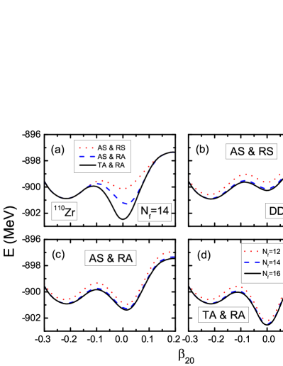
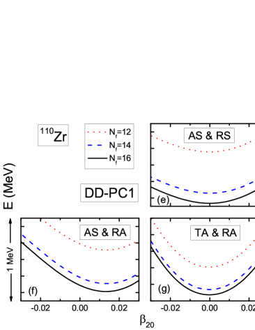
The calculated physical observables should converge as the truncation $N_{f}\rightarrow\infty$. In Fig. 1, we show the one-dimensional (1D) potential energy curve of ¹¹⁰Zr around the ground state with axial symmetry and reflection symmetry, axial symmetry and reflection asymmetry, and nonaxial and reflection asymmetry imposed, respectively. The effective interaction DD-PC1 Nikšić et al. (2008) is used. Calculations with different truncations ($N_{f}=12$, 14, and 16) are depicted by dotted, dashed, and solid curves, respectively. As shown in the upper panel of Fig. 1, the predicted ground state shape of ¹¹⁰Zr is oblate with $\beta_{20}\approx-0.2$ when both axial and reflection symmetries are imposed. There is another minimum around $\beta_{20}=0$. The energy of this minimum is reduced by about 1 MeV when the axial octupole deformation ($\beta_{30}$) is included, while the energy gain is about 2 MeV when the nonaxial octupole deformation ($\beta_{32}$) is included. As a result, the ground state changes to be $\beta_{20}\approx 0$. To see more clearly the truncation errors, we have amplified the figure near $\beta_{20}=0$. We can see that for ¹¹⁰Zr, the energy changes about 400 keV when $N_{f}$ increases from 12 to 14; further increasing $N_{f}$ from 14 to 16, the energy changes only about 100 keV. Furthermore, from Fig. 1, one can find that the inaccuracy caused by the finite basis size is almost independent of the imposed symmetry (in this case, independent of whether the axial or nonaxial deformations, reflection symmetric or reflection asymmetric deformations are included). This means a good convergence and $N_{f}=14$ is sufficient in this mass region.

Figure 2: The binding energy (a) and $\beta_{32}$ deformation (b) of ¹¹⁰Zr from MDC-RHB calculations with different truncations made in the Fourier expansion of densities and potentials. The calculations are performed with $N_{f}=14$. The functional DD-PC1 is used in the MDC-RHB calculations.

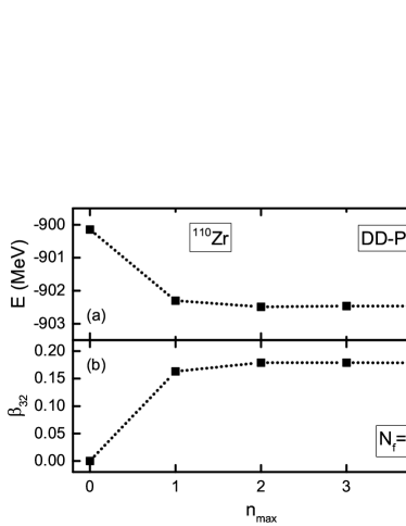
For axially symmetric nuclei where potentials and densities $f(\rho,\varphi,z)\equiv f(\rho,z)$ are independent of the azimuthal angle $\varphi$, the Fourier coefficient $f_{n}(\rho,z)=0$ when $n\geq 1$. For nonaxial nuclei, $f_{n}(\rho,z)\neq 0$ when $n\geq 1$. Therefore, $n$ characterizes the nonaxiality of potentials and densities. In practical calculations, the Fourier series in Eq. (28) has to be truncated, i.e., $n\leq n_{\rm{max}}$. To study the dependence of the calculated results on $n_{\rm{max}}$, we show the binding energy and nonaxial $\beta_{32}$ deformation parameter of ¹¹⁰Zr calculated with different $n_{\rm{max}}$ in Fig. 2. As shown in Fig. 2(b), if all $f_{n}$’s with $n\geq 1$ are omitted ($n_{\rm{max}}=0$), the nucleus remains axial and $\beta_{32}=0$. The convergence of the binding energy and $\beta_{32}$ with $n_{\rm{max}}$ increasing is very fast. The results obtained with $n_{\rm{max}}=2$ are very precise already; the energy gain when $n_{\rm{max}}$ increases from 2 to 3 is only around 30 keV. In practical calculations, $n_{\rm{max}}$ is determined automatically by the relation $2n_{\rm{max}}=K_{\rm{max}}-K_{\rm{min}}$, where $K_{\rm{max}}$ ($K_{\rm{min}}$) is the largest (smallest) $K$ in the truncated ADHO basis. This is sufficiently large for all of results discussed here.

III.2 Neutron-rich even-even Zr isotopes

Figure 3: (Color online) Potential energy curves ($E\sim\beta_{20}$) for Zr isotopes. The energy is normalized with respect to the energy minimum with $\beta_{20}<0$ for each nucleus. The dotted line denotes results with axial symmetry (AS) and reflection symmetry (RS) imposed, the dash-dotted line denotes results restricted to AS and reflection asymmetry (RA), while the solid line represents results with both AS and RS broken, i.e., with triaxial (TA) deformation and RA. The functional DD-PC1 is used in MDC-RHB calculations.

We calculate one-dimensional (1D) potential energy curves ($E\sim\beta_{20}$) for even-even Zr nuclei with $100\leq A\leq 114$. The functionals DD-PC1 Nikšić et al. (2008) and PC-PK1 Zhao et al. (2010) are used. To investigate different roles played by the nonaxiality and reflection asymmetry, calculations are preformed with different symmetries imposed: (i) axial and reflection symmetry, (ii) axial symmetry and reflection asymmetry, and (iii) nonaxial and reflection asymmetry, and the results are denoted by dotted, dash-dotted, and solid lines, respectively.

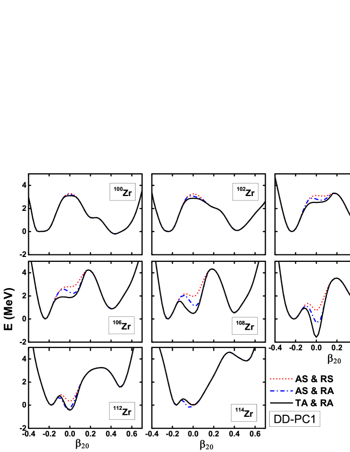
First we focus on 1D potential energy curves obtained with DD-PC1, which are shown in Fig. 3. If nuclear shapes are restricted to be axial and reflection symmetric (red dotted line), a prolate ground state with $\beta_{20}\approx 0.4$ coexisting with an oblate minimum with $\beta_{20}\approx-0.2$ is obtained for ¹⁰⁰Zr. This is consistent with the experimental observations Mach et al. (1990); Hwang et al. (2006a); Hua et al. (2004); Cheifetz et al. (1970). For ^102-114Zr, the ground state shapes are predicted to be oblate with $\beta_{20}\approx-0.2$. As neutron number increases, the energy of the minimum with $\beta_{20}>0$ increases. A minimum with $\beta_{20}\approx 0$ is developed starting from ¹⁰⁶Zr. This minimum becomes lower in energy and the pocket becomes deeper with the neutron number increasing.

If nuclei are allowed to be reflection asymmetric but axial symmetric, one obtains 1D potential energy curves, denoted by blue dash-dotted lines in Fig. 3. The $\beta_{30}$ deformation is involved around $\beta_{20}=0$ for all of the nuclei investigated here. As a result, a minimum develops for ¹⁰⁴Zr around $\beta_{20}=0$. The energy of the minimum with $\beta_{20}\approx 0$ for ^106-114Zr is lowered substantially by the $\beta_{30}$ distortion. Due to this lowering effect, the energy of the minimum with pear-like shape ($\beta_{20}\approx 0$, $\beta_{30}\neq 0$) is lower than the minimum with oblate or prolate shape for ¹¹⁰Zr, ¹¹²Zr, and ¹¹⁴Zr. This lowering effect is also found in Skyrme HFB+BCS calculations Zberecki et al. (2009). The $\beta_{30}$ deformation is not important either around the oblate minimum ($\beta_{20}\approx-0.2$) or around the prolate minimum ($\beta_{20}\approx 0.4$). Note that these results are different from those presented in Ref. Agbemava et al. (2016) where the octupole deformation is found only in the ground state of ¹¹²Zr with the functional DD-PC1. Such differences are mainly caused by different pairing strengths used in these two works. We have checked that if we use the pairing strengths given in Ref. Agbemava et al. (2016), i.e., $G_{n}=G_{p}=1.12G_{0}$ with $G_{0}=738$ MeV$\cdot$fm³, we can get the same results as Ref. Agbemava et al. (2016).

When the $\beta_{32}$ deformation is allowed in the calculations, both axial and reflection symmetries are broken. As seen in Fig. 3, the $\beta_{32}$ deformation changes very much the energy around $\beta_{20}=0$ (the black solid line). Similar to the cases discussed in the previous paragraph about the inclusion of $\beta_{30}$, a minimum also develops for ¹⁰⁴Zr around $\beta_{20}=0$. However, the $\beta_{32}$ distortion effect is more pronounced than that of the $\beta_{30}$ deformation for most of these nuclei. The energy of the minimum with $\beta_{20}\approx 0$ for ^106-112Zr is lowered substantially. A tetrahedral ground state is predicted for ^110,112Zr. For ¹¹⁴Zr, the predicted pear-like shape is lower in energy than the tetrahedral shape. From Fig. 3, we know that the $\beta_{32}$ distortion effect is the most pronounced for ¹¹⁰Zr, where the inclusion of the $\beta_{32}$ deformation lowers the energy of the minimum around $\beta_{20}=0$ by about 2 MeV. Similar to the situation of $\beta_{30}$, the $\beta_{32}$ deformation is important neither around the oblate minimum ($\beta_{20}\approx-0.2$) nor around the prolate minimum ($\beta_{20}\approx 0.4$). The obtained ground state deformation parameters as well as the binding energies with DD-PC1 for ^110-114Zr are listed in Table 2. The corresponding available experimental values are also included for comparison. The predicted energies of various minima (with respect to the corresponding ground state energy) are presented in Table 3.

Table 2: The quadrupole deformation $\beta_{20}$, axial octupole deformation $\beta_{30}$, nonaxial octupole deformation $\beta_{32}$, and hexadecapole deformation $\beta_{40}$ together with binding energies $E_{\mathrm{cal}}$ for the ground states of Zr isotopes obtained in MDC-RHB calculations with the functional DD-PC1. $E_{\mathrm{exp}}$ denotes experimental binding energies taken from Ref. Wang et al. (2012). $\beta_{\mathrm{exp}}$ represents experimental quadrupole deformations taken from Ref. Raman et al. (2001). The data with “*” stand for estimated values Wang et al. (2012). All energies are in MeV.

Nucleus	$\beta_{20}$	$\beta_{30}$	$\beta_{32}$	$\beta_{40}$	$E_{\rm cal}$	$\beta_{\rm exp}$	$E_{\rm exp}$
100Zr	$0.44$	$0.00$	$0.00$	$0.22$	$-851.90$	$0.36$	$-852.22$
102Zr	$-0.24$	$0.00$	$0.00$	$0.04$	$-863.10$	$0.43$	$-863.57$
104Zr	$-0.24$	$0.00$	$0.00$	$0.02$	$-874.01$	$0.47$	$-873.85$
106Zr	$-0.24$	$0.00$	$0.00$	$0.01$	$-884.18$		$-883.19^{*}$
108Zr	$-0.24$	$0.00$	$0.00$	$0.00$	$-893.16$		$-891.76^{*}$
110Zr	$0.00$	$0.00$	$0.18$	$-0.04$	$-902.46$		$-899.47^{*}$
112Zr	$0.00$	$0.00$	$0.13$	$-0.02$	$-908.79$		$-906.53^{*}$
114Zr	$-0.04$	$0.13$	$0.00$	$0.02$	$-915.50$

Table 3: The binding energy (relative to the ground state) for various energy minima (when they exist) in Zr isotopes obtained in the MDC-RHB calculations with the functional DD-PC1. All energies are in MeV.

Nucleus	100Zr	102Zr	104Zr	106Zr	108Zr	110Zr	112Zr	114Zr
Oblate	$0.21$	$0.00$	$0.00$	$0.00$	$0.00$	$1.58$	$0.44$	$0.19$
Pear-like			$2.72$	$2.22$	$1.12$	$1.25$	$0.08$	$0.00$
Tetrahedral			$2.53$	$1.85$	$0.49$	$0.00$	$0.00$	$0.20$
Prolate	$0.00$	$0.10$	$0.63$	$0.89$	$0.53$	$2.55$	$2.02$	$4.02$

Figure 4: The single-particle levels near the Fermi surface for protons (a) and neutrons (b) of ¹¹⁰Zr as functions of $\beta_{32}$ with $\beta_{20}$ fixed at zero. The functional DD-PC1 is used in the MDC-RHB calculations.

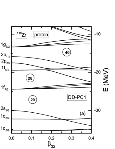
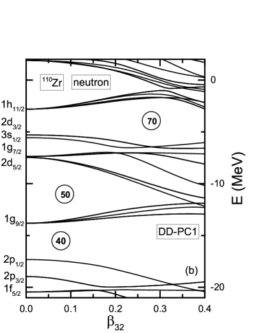
From Fig. 3 and Table 2, one finds that the ground states of ^100-108Zr are well deformed with large quadrupole deformation. For ¹⁰⁸Zr, a tetrahedral isomeric state is also predicted. The ground states of ^110,112Zr are predicted to have tetrahedral shape and the most pronounced effect from the $\beta_{32}$ distortion is in ¹¹⁰Zr with the functional DD-PC1. The formation of the tetrahedral ground state around ¹¹⁰Zr can be traced back to the large energy gaps at $Z=40$ and $N=70$ in the single-particle levels when $\beta_{32}$ deformation is included. In Fig. 4, we show the single-particle levels of ¹¹⁰Zr near the Fermi surface as functions of $\beta_{32}$ with $\beta_{20}$ fixed at zero. Due to the tetrahedral symmetry, the single-particle levels split into multiplets with degeneracies equal to the irreducible representations of the $T^{D}_{d}$ group. For example, the spherical levels with $j=1/2$ and $j=3/2$ are two-fold and four-fold degenerate and they can be reduced to the two-dimensional (2D) irreducible representation $E_{1}^{\prime}$ and four-dimensional (4D) irreducible representation $G^{\prime}$ of the $T^{D}_{d}$ group, respectively. Such degeneracies are kept as $\beta_{32}$ increases. The spherical levels with $j=5/2$ can be reduced to the 2D irreducible representation $E_{2}^{\prime}$ and 4D irreducible representation $G^{\prime}$ of the $T^{D}_{d}$ group. These levels split into two levels with degeneracies 2 and 4, respectively, as $\beta_{32}$ increases. The reduction of spherical levels (up to $j=11/2$) to the irreducible representation of the $T^{D}_{d}$ group are listed in Table 4. For protons, as shown in Fig. 4(a), the magic gap $Z\simeq 20$ is enhanced while the gap at $Z\simeq 28$ is suppressed as $\beta_{32}$ increases. At $Z\simeq 40$ a large energy gap shows up with $\beta_{32}$ increasing. From Fig. 4(b) we can see that large energy gaps appears at $N\simeq 40$ and 70 while the spherical magic gap around $N=50$ is suppressed as $\beta_{32}$ increases. Due to large energy gaps at $Z\simeq 40$ and $N\simeq 70$, a strong $\beta_{32}$ effect is expected for ¹¹⁰Zr and nearby nuclei.

Table 4: The reductions of the spherical levels (up to $j=11/2$) to the irreducible representations of the $T^{D}_{d}$ group. The two 2D irreducible representations of the $T^{D}_{d}$ group are denoted by $E_{1}^{\prime}$ and $E_{2}^{\prime}$, the 4D irreducible representation of the $T^{D}_{d}$ group is denoted by $G^{\prime}$.

$j$	Irreducible representations of $T^{D}_{d}$ group
1/2	$E_{1}^{\prime}$
3/2	$G^{\prime}$
5/2	$E_{2}^{\prime}+G^{\prime}$
7/2	$E_{1}^{\prime}+E_{2}^{\prime}+G^{\prime}$
9/2	$E_{1}^{\prime}+2G^{\prime}$
11/2	$E_{1}^{\prime}+E_{2}^{\prime}+2G^{\prime}$

Figure 5: (Color online)  The proton and neutron pairing energies of ¹¹⁰Zr as functions of $\beta_{20}$. The dotted line denotes the results with the axial symmetry (AS) and reflection symmetry (RS) imposed, the dash-dotted line denotes the results restricted to the AS and reflection asymmetry (RA), while the solid line represents the results with both triaxial (TA) and RA shapes allowed. The functional DD-PC1 is used in the MDC-RHB calculations.

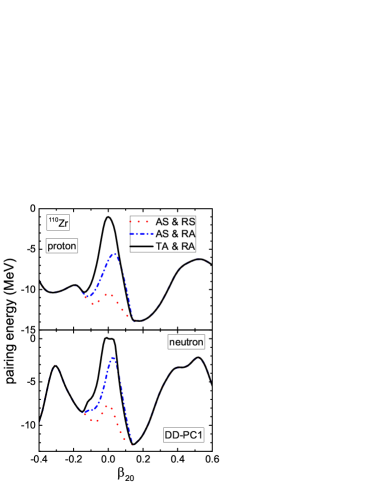
In Fig. 5 we show the proton and neutron pairing energies of ¹¹⁰Zr calculated with the functional DD-PC1. The changes of the pairing energy as a function of $\beta_{20}$ are due to the variations of single-particle level density near the Fermi surface when $\beta_{20}$ changes: lower level density near the Fermi surface usually leads to weaker pairing effects. When $\beta_{30}$ and $\beta_{32}$ deformations are not included, the weakest pairing effects are found around the prolate minimum (note that the three curves overlap around this minimum). However, the inclusion of $\beta_{30}$ or $\beta_{32}$ reduces the proton and neutron pairing effects around $\beta_{20}=0$ a lot. Especially for the case of $\beta_{32}$, both proton and neutron paring energies almost vanish around $\beta_{20}=0$, due to the large energy gap developed at $Z\simeq 40$ and $N\simeq 70$.

Figure 6: (Color online) The potential energy surfaces of ^106-114Zr in the $(\beta_{30},\beta_{32})$ plane with $\beta_{20}$ fixed at zero. The contour interval is 0.1 MeV. The functional DD-PC1 is used in the MDC-RHB calculations.

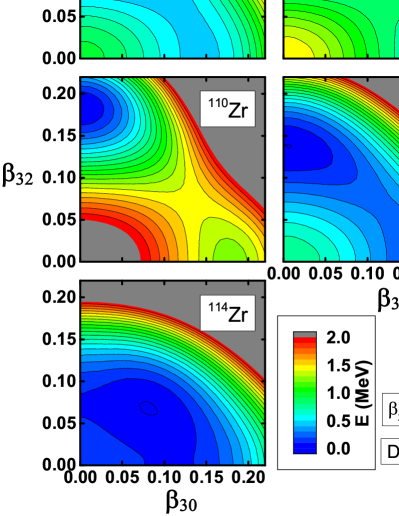
From the above discussions, we know that the inclusion of $\beta_{30}$ and $\beta_{32}$ deformations can reduce the energies around $\beta_{20}=0$ for most of the neutron-rich Zr isotopes investigated here. As a result, with the functional DD-PC1, tetrahedral ground states and pear-like isomeric states are predicted for ^110,112Zr and a pear-like ground state and a tetrahedral isomeric state are predicted for ¹¹⁴Zr. To further investigate the properties and the relation between these two minima, we calculate the potential energy surfaces (PES) of ^106-114Zr in the $(\beta_{30},\beta_{32})$ plane with $\beta_{20}$ fixed at zero and show them in Fig. 6. It is clearly seen that the pockets around tetrahedral minima are deeper than those around pear-like minima for ^106-112Zr. For example, the minimum with $\beta_{30}\approx 0.15$ of ¹¹⁰Zr is 1.25 MeV higher than the tetrahedral minimum with $\beta_{32}\approx 0.15$. From Fig. 6, one finds that the barriers separating the pear-like and the tetrahedral minima are very low. For ¹⁰⁶Zr, the barrier is almost invisible. For ¹⁰⁸Zr and ¹¹²Zr, the barrier heights are less than 0.2 MeV. For ¹¹⁰Zr, the barrier is higher, but still less than 0.3 MeV. In this sense, the pear-like isomeric states are rather unstable and may hardly be observed for the nuclei discussed here.

We also preformed similar calculations with the functional PC-PK1. By examining the obtained 1D potential energy curves and 2D potential energy surfaces, it is found that with this functional and the same pairing strength as used in calculations with the functional DD-PC1 (i.e., $G_{n}=G_{0}$, $G_{p}=1.12G_{0}$ with $G_{0}=728$ MeV$\cdot$fm³), the tetrahedral and octupole deformations have less influence on Zr isotopes than they do with DD-PC1. In this sense, the tetrahedral and octupole deformation effects are functional dependent. With these two shape degrees of freedom considered, the potential energy surfaces become softer around the local minima with $\beta_{20}\approx 0$. The most pronounced effects from the tetrahedral or octupole distortions happen in ¹¹⁰Zr for which a spherical shape is already obtained under the assumption of axial and reflection symmetries. In the AS & RA calculations, the ground state minimum for ¹¹⁰Zr is lowered by about 0.1 MeV and in the TA & RA calculations, the minimum corresponding to the tetrahedral shape is lower by about 0.1 MeV than that corresponds to an octupole shape.

Experimentally, low-lying spectra for even-$A$ Zr isotopes have been established, from which it has been concluded that ^{100,102,104,106,108}Zr are well deformed. However, there has been no such experimental information for ¹¹⁰Zr. In some theoretical investigations (see, e.g., Ref. Togashi et al. (2016)) it is predicted that ¹¹⁰Zr is also well deformed. In our calculations, ¹¹⁰Zr is predicted to be tetrahedral because of the strong effects of shell closures around $Z\simeq 40$ and $N\simeq 70$.

IV Summary

We have developed a multidimensionally constrained relativistic Hartree-Bogoliubov (MDC-RHB) model in which the pairing correlations are taken into account with the Bogoliubov transformation. In this model, the nuclear shape is assumed to be invariant under the reversion of $x$ and $y$ axes, thus, all shape degrees of freedom $\beta_{\lambda\mu}$ with even $\mu$ are included self-consistently. A separable pairing force of finite range is adopted in this model. We solve the RHB equation in an axially deformed harmonic oscillator (ADHO) basis. The convergence of the calculated results against the basis truncation is studied and it is shown that a reasonably large ADHO basis is able to provide a desired accuracy.

We have calculated the potential energy curves ($E\sim\beta_{20}$) of neutron-rich even-even Zr isotopes with the MDC-RHB model. It is found that the $\beta_{32}$ deformation plays a very important role in the isomeric or ground states of these nuclei, especially for nuclei around $N=70$. The ground state shape of ¹¹⁰Zr is predicted to be tetrahedral with both functionals DD-PC1 and PC-PK1. ¹¹²Zr is also predicted to have a tetrahedral ground state with the functional DD-PC1. We investigated the evolution of single-particle levels in ¹¹⁰Zr as a function of the $\beta_{32}$ deformation. It is found that there are large energy gaps at $Z\simeq 40$ and $N\simeq 70$ which are responsible for the strong $\beta_{32}$ distortion effect. The inclusion of $\beta_{30}$ deformation can also reduce the energy around $\beta_{20}=0$ and lead to minima with pear-like shapes for nuclei around ¹¹⁰Zr, but these minima are rather shallow. By examining two-dimensional potential energy surfaces in the ($\beta_{30},\beta_{32}$) plane with $\beta_{20}$ fixed at zero, we found that the barrier separating the two minima with nonzero $\beta_{32}$ or nonzero $\beta_{30}$ is quite low.

Appendix A Calculation of the pairing fields

The separable pairing force of finite range in the coordinate space reads

$$V(\bm{r}_{1}\sigma_{1},\bm{r}_{2}\sigma_{2},\bm{r}_{1}^{\prime}\sigma_{1}^{\prime},\bm{r}_{2}^{\prime}\sigma_{2}^{\prime}) = -G\delta(\bm{R}-\bm{R}^{\prime})P(r)P(r^{\prime})$$ (43)

$$\times\frac{1}{2}(1-P_{\sigma}),$$

where $\bm{R}=(\bm{r}_{1}+\bm{r}_{2})/2$ and $\bm{r}=\bm{r}_{1}-\bm{r}_{2}$ are the center-of-mass and relative coordinates, respectively. The corresponding matrix element in the axially deformed harmonic oscillator (ADHO) basis is

$$V_{12,1^{\prime}2^{\prime}} = \sum_{\sigma_{1}\sigma_{2}}\sum_{\sigma_{1}^{\prime}\sigma_{2}^{\prime}}\int d^{3}\bm{r}_{1}d^{3}\bm{r}_{2}d^{3}\bm{r}_{1}^{\prime}d^{3}\bm{r}_{2}^{\prime}\Phi_{1}^{*}(\bm{r}_{1}\sigma_{1})\Phi_{2}^{*}(\bm{r}_{2}\sigma_{2})$$

$$\times V(\bm{r}_{1}\sigma_{1},\bm{r}_{2}\sigma_{2},\bm{r}_{1}^{\prime}\sigma_{1}^{\prime},\bm{r}_{2}^{\prime}\sigma_{2}^{\prime})\Phi_{1^{\prime}}(\bm{r}_{1}^{\prime}\sigma_{1}^{\prime})\Phi_{2^{\prime}}(\bm{r}_{2}^{\prime}\sigma_{2}).$$

Referring to the structure of the basis wave functions Eq. (II), $V_{12,1^{\prime}2^{\prime}}$ can be written as a product of integrals and sums,

$$V_{12,1^{\prime}2^{\prime}}=(C_{1}C_{2})^{*}(C_{1^{\prime}}C_{2^{\prime}})V_{12,1^{\prime}2^{\prime}}^{\sigma}V_{12,1^{\prime}2^{\prime}}^{z}V_{12,1^{\prime}2^{\prime}}^{\rho},$$ (45)

with

$$V_{12,1^{\prime}2^{\prime}}^{\sigma} = \sum_{\begin{subarray}{c}\sigma_{1}\sigma_{2}\\ \sigma_{1}^{\prime}\sigma_{2}^{\prime}\end{subarray}}\chi_{s_{1}}(\sigma_{1})\chi_{s_{2}}(\sigma_{2})\frac{1}{2}(1-P_{\sigma})\chi_{s_{1}^{\prime}}(\sigma_{1}^{\prime})\chi_{s_{2}^{\prime}}(\sigma_{2}^{\prime})$$ (46)

$$= \frac{1}{2}(2s_{1}\delta_{\sigma_{1},\bar{\sigma_{2}}})(2s_{1}^{\prime}\delta_{\sigma_{1}^{\prime},\bar{\sigma_{2}^{\prime}}}),$$

$$V_{12,1^{\prime}2^{\prime}}^{z}= \int dz_{1}dz_{2}dz_{1}^{\prime}dz_{2}^{\prime}\phi_{n_{z_{1}}}(z_{1})\phi_{n_{z_{2}}}(z_{2})$$ (47)

$$\times\left[\delta(Z-Z^{\prime})P_{z}(z)P_{z}(z^{\prime})\right]\phi_{n_{z_{1}}^{\prime}}(z_{1}^{\prime})\phi_{n_{z_{2}}^{\prime}}(z_{2}^{\prime})$$

$$= \sqrt{2}\sum_{N_{z}}\left(\sum_{n}M_{N_{z}n}^{n_{z_{1}}n_{z_{2}}}A_{n}\right)\left(\sum_{n}M_{N_{z}n}^{n_{z_{1}}^{\prime}n_{z_{2}}^{\prime}}A_{n}\right),$$

$$V_{12,1^{\prime}2^{\prime}}^{\rho} = \int d^{2}\bm{\rho}_{1}d^{2}\bm{\rho}_{2}d^{2}\bm{\rho}_{1}^{\prime}d^{2}\bm{\rho}_{2}^{\prime}$$ (48)

$$\times R_{n_{\rho_{1}}}^{m_{l_{1}}}(\rho_{1})R_{n_{\rho_{2}}}^{m_{l_{2}}}(\rho_{2})\frac{1}{2\pi}e^{-i(m_{l_{1}}\varphi_{1}+m_{l_{2}}\varphi_{2})}$$

$$\times\left[\delta(\bm{\rho}-\bm{\rho}^{\prime})P_{\rho}(\rho)P_{\rho}(\rho^{\prime})\right]$$

$$\times R_{n_{\rho_{1}}^{\prime}}^{m_{l_{1}}^{\prime}}(\rho_{1})R_{n_{\rho_{2}}^{\prime}}^{m_{l_{2}}^{\prime}}(\rho_{2})\frac{1}{2\pi}e^{i(m_{l_{1}}^{\prime}\varphi_{1}+m_{l_{2}}^{\prime}\varphi_{2})}$$

$$= \sqrt{2}\sum_{N_{\rho}M_{\rho}}\left(\sum_{n}M_{N_{\rho}M_{\rho}n0}^{n_{\rho_{1}}m_{l_{1}}n_{\rho_{2}}m_{l_{2}}}B_{n}\right)$$

$$\times\left(\sum_{n}M_{N_{\rho}M_{\rho}n0}^{n_{\rho_{1}}^{\prime}m_{l_{1}}^{\prime}n_{\rho_{2}}^{\prime}m_{l_{2}}^{\prime}}B_{n}\right),$$

where

$$A_{n} = \int_{-\infty}^{\infty}\phi_{n}(z)P_{z}(\sqrt{2}z)dz,$$

$$B_{n} = \sqrt{2\pi}\int_{0}^{\infty}P_{\rho}(\sqrt{2}\rho)R_{n}^{0}(\rho)\rho d\rho,$$ (49)

are constants. All these terms are in separable forms; so is the matrix element

$$V_{12,1^{\prime}2^{\prime}}=\sum_{N_{z}N_{\rho}M_{\rho}}\left(W_{12}^{N_{z}N_{\rho}M_{\rho}}\right)^{*}W_{1^{\prime}2^{\prime}}^{N_{z}N_{\rho}M_{\rho}},$$ (50)

where

$$W_{12}^{N_{z}N_{\rho}M_{\rho}} = (C_{1}C_{2})(2s_{1}\delta_{\sigma_{1},\bar{\sigma_{2}}})\left(\sum_{n}M_{N_{z}n}^{n_{z_{1}}n_{z_{2}}}A_{n}\right)$$ (51)

$$\times\left(\sum_{n}M_{N_{\rho}M_{\rho}n0}^{n_{\rho_{1}}m_{l_{1}}n_{\rho_{2}}m_{l_{2}}}B_{n}\right).$$

The Talmi-Moshinski brackets are given in the next appendix.

Appendix B The Talmi-Moshinski brackets

As usual the Talmi-Moshinski brackets are calculated by the generating function method. Here we only show the final results and the details can be found in Ref. Chaos-Cador and Ley-Koo (2004).

The one-dimensional Talmi-Moshinski bracket reads

$$M_{N_{z}n_{z}}^{n_{z_{1}}n_{z_{2}}} = \int_{-\infty}^{\infty}dz_{1}dz_{2}\phi_{n_{z_{1}}}(z_{1})\phi_{n_{z_{2}}}(z_{2})\phi_{N_{z}}(z_{+})\phi_{n_{z}}(z_{-})$$ (56)

$$= \frac{1}{\sqrt{2^{N_{z}+n_{z}}}}\sqrt{\frac{n_{z_{1}}!n_{z_{2}}!}{N_{z}!n_{z}!}}\delta_{n_{z_{1}}+n_{z_{2}},N_{z}+n_{z}}$$

$$\times\sum_{s=0}^{n_{z}}\left(-1\right)^{s}\left(\begin{array}[]{c}N_{z}\\ n_{z_{1}}-n_{z}+s\end{array}\right)\left(\begin{array}[]{c}n_{z}\\ s\end{array}\right),$$

where $z_{+}=\frac{1}{\sqrt{2}}(z_{1}+z_{2})$ and $z_{-}=\frac{1}{\sqrt{2}}(z_{1}-z_{2})$.

The two-dimensional Talmi-Moshinski bracket is

$$M_{NMnm}^{n_{1}m_{1}n_{2}m_{2}} = \int_{0}^{\infty}\rho_{1}d\rho_{1}\int_{0}^{2\pi}d\varphi_{1}\int_{0}^{\infty}\rho_{2}d\rho_{2}\int_{0}^{2\pi}d\varphi_{2}R_{n_{1}}^{m_{1}}(\rho_{1})e^{-im_{1}\varphi_{1}}R_{n_{2}}^{m_{2}}(\rho_{2})e^{-im_{2}\varphi_{2}}R_{N}^{M}(\rho_{+})e^{iM\varphi_{+}}R_{n}^{m}(\rho_{-})e^{im\varphi_{-}}$$ (65)

$$= \delta_{M+m,m_{1}+m_{2}}\delta_{2n_{1}+|m_{1}|+2n_{2}+|m_{2}|,2N+|M|+2n+|m|}\frac{(-1)^{n_{1}+n_{2}+N+n}}{\sqrt{2^{2n_{1}+|m_{1}|+2n_{2}+|m_{2}|}}}\sqrt{\frac{N!(N+|M|)!n!(n+|m|)!}{n_{1}!(n_{1}+|m_{1}|)!n_{2}!(n_{2}+|m_{2}|)!}}$$

$$\times\sum_{\begin{subarray}{c}p_{1},q_{1},r_{1},s_{1}\\ p_{2},q_{2},r_{2},s_{2}\end{subarray}}^{n_{1}n_{2}}\sum_{t_{1}t_{2}}^{|m_{1}||m_{2}|}(-1)^{r_{2}+s_{2}+|m_{2}|-t_{2}}\delta_{p_{2}r_{2}s_{2}t_{2}}^{p_{1}r_{1}s_{1}t_{1}}\left(\begin{array}[]{c}|m_{1}|\\ t_{1}\end{array}\right)\left(\begin{array}[]{c}|m_{2}|\\ t_{2}\end{array}\right)\left(\begin{array}[]{cccc}&n_{1}\\ p_{1}&q_{1}&r_{1}&s_{1}\end{array}\right)\left(\begin{array}[]{cccc}&n_{2}\\ p_{2}&q_{2}&r_{2}&s_{2}\end{array}\right),$$

where the variables $(\rho_{\pm},\varphi_{\pm})$ are defined as

$$\rho_{\pm}\cos\varphi_{\pm} = \frac{1}{\sqrt{2}}(\rho_{1}\cos\varphi_{1}\pm\rho_{2}\cos\varphi_{2}),$$

$$\rho_{\pm}\sin\varphi_{\pm} = \frac{1}{\sqrt{2}}(\rho_{1}\sin\varphi_{1}\pm\rho_{2}\sin\varphi_{2}).$$ (67)

The multinomial coefficients are

$$\left(\begin{array}[]{ccccc}&&q\\ p_{1}&p_{2}&p_{3}&\cdots&p_{n}\end{array}\right)=\delta_{\sum_{k}p_{k},q}\frac{q!}{\prod_{k=1}^{n}p_{k}},$$ (68)

and the Kronecker $\delta$’s are

$$\delta_{p_{2}r_{2}s_{2}t_{2}}^{p_{1}r_{1}s_{1}t_{1}}=\left\{\begin{array}[]{c}\delta_{t_{1}+t_{2},N-(p_{1}+s_{1})-(p_{2}+s_{2})+(|M|+M)/2}\delta_{0,N-(p_{1}+r_{1})-(p_{2}+r_{2})+\frac{1}{2}(|M|-M)},\quad m_{1}m_{2}\geq 0,\\ \delta_{t_{1},N-(p_{1}+s_{1})-(p_{2}+s_{2})+(|M|+M)/2}\delta_{t_{2},N-(p_{1}+r_{1})-(p_{2}+r_{2})+(|M|-M)/2},\quad m_{1}m_{2}\leq 0.\end{array}\right.$$ (69)

References

- Bohr and Mottelson (1969) A. Bohr and B. R. Mottelson, Nuclear Structure, 1st ed., Vol. I (Benjamin, New York, 1969).
- Bohr and Mottelson (1975) A. Bohr and B. R. Mottelson, Nuclear Structure, 1st ed., Vol. II (Benjamin, New York, 1975).
- Frauendorf and Meng (1997) S. Frauendorf and J. Meng, Nucl. Phys. A 617, 131 (1997).
- Odegard et al. (2001) S. W. Odegard, G. B. Hagemann, D. R. Jensen, M. Bergstroem, B. Herskind, G. Sletten, S. Toermaenen, J. N. Wilson, P. O. Tjom, I. Hamamoto, K. Spohr, H. Huebel, A. Goergen, G. Schoenwasser, A. Bracco, S. Leoni, A. Maj, C. M. Petrache, P. Bednarczyk, and D. Curien, Phys. Rev. Lett. 86, 5866 (2001).
- Starosta et al. (2001) K. Starosta, T. Koike, C. J. Chiara, D. B. Fossan, D. R. LaFosse, A. A. Hecht, C. W. Beausang, M. A. Caprio, J. R. Cooper, R. Krucken, J. R. Novak, N. V. Zamfir, K. E. Zyromski, D. J. Hartley, D. L. Balabanski, J.-y. Zhang, S. Frauendorf, and V. I. Dimitrov, Phys. Rev. Lett. 86, 971 (2001).
- Meng et al. (2006a) J. Meng, J. Peng, S. Q. Zhang, and S.-G. Zhou, Phys. Rev. C 73, 037303 (2006a).
- Ayangeakaa et al. (2013) A. D. Ayangeakaa, U. Garg, M. D. Anthony, S. Frauendorf, J. T. Matta, B. K. Nayak, D. Patel, Q. B. Chen, S. Q. Zhang, P. W. Zhao, B. Qi, J. Meng, R. V. F. Janssens, M. P. Carpenter, C. J. Chiara, F. G. Kondev, T. Lauritsen, D. Seweryniak, S. Zhu, S. S. Ghugre, and R. Palit, Phys. Rev. Lett. 110, 172504 (2013).
- Lieder et al. (2014) E. O. Lieder, R. M. Lieder, R. A. Bark, Q. B. Chen, S. Q. Zhang, J. Meng, E. A. Lawrie, J. J. Lawrie, S. P. Bvumbi, N. Y. Kheswa, S. S. Ntshangase, T. E. Madiba, P. L. Masiteng, S. M. Mullins, S. Murray, P. Papka, D. G. Roux, O. Shirinda, Z. H. Zhang, P. W. Zhao, Z. P. Li, J. Peng, B. Qi, S. Y. Wang, Z. G. Xiao, and C. Xu, Phys. Rev. Lett. 112, 202502 (2014).
- Kuti et al. (2014) I. Kuti, Q. B. Chen, J. Timar, D. Sohler, S. Q. Zhang, Z. H. Zhang, P. W. Zhao, J. Meng, K. Starosta, T. Koike, E. S. Paul, D. B. Fossan, and C. Vaman, Phys. Rev. Lett. 113, 032501 (2014).
- Tonev et al. (2014) D. Tonev, M. S. Yavahchova, N. Goutev, G. de Angelis, P. Petkov, R. K. Bhowmik, R. P. Singh, S. Muralithar, N. Madhavan, R. Kumar, M. Kumar Raju, J. Kaur, G. Mohanto, A. Singh, N. Kaur, R. Garg, A. Shukla, T. K. Marinov, and S. Brant, Phys. Rev. Lett. 112, 052501 (2014).
- Liu et al. (2016) C. Liu, S. Y. Wang, R. A. Bark, S. Q. Zhang, J. Meng, B. Qi, P. Jones, S. M. Wyngaardt, J. Zhao, C. Xu, S.-G. Zhou, S. Wang, D. P. Sun, L. Liu, Z. Q. Li, N. B. Zhang, H. Jia, X. Q. Li, H. Hua, Q. B. Chen, Z. G. Xiao, H. J. Li, L. H. Zhu, T. D. Bucher, T. Dinoko, J. Easton, K. Juhász, A. Kamblawe, E. Khaleel, N. Khumalo, E. A. Lawrie, J. J. Lawrie, S. N. T. Majola, S. M. Mullins, S. Murray, J. Ndayishimye, D. Negi, S. P. Noncolela, S. S. Ntshangase, B. M. Nyakó, J. N. Orce, P. Papka, J. F. Sharpey-Schafer, O. Shirinda, P. Sithole, M. A. Stankiewicz, and M. Wiedeking, Phys. Rev. Lett. 116, 112501 (2016).
- Bengtsson et al. (1984) R. Bengtsson, H. Frisk, F. R. May, and J. A. Pinston, Nucl. Phys. A 415, 189 (1984).
- Liu et al. (1995) Y. Liu, Y. Ma, H. Yang, and S. Zhou, Phys. Rev. C 52, 2514 (1995).
- Liu et al. (1996) Y. Liu, J. Lu, Y. Ma, S. Zhou, and H. Zheng, Phys. Rev. C 54, 719 (1996).
- Zhou et al. (1996) S. G. Zhou, Y. Z. Liu, Y. J. Ma, and C. X. Yang, J. Phys. G: Nucl. Phys. 22, 415 (1996).
- Riedinger et al. (1997) L. L. Riedinger, H. Q. Jin, W. Reviol, J.-Y. Zhang, R. A. Bark, G. B. Hagemann, and P. B. Semmes, Prog. Part. Nucl. Phys. 38, 251 (1997).
- Liu et al. (1998) Y. Liu, J. Lu, Y. Ma, G. Zhao, H. Zheng, and S. Zhou, Phys. Rev. C 58, 1849 (1998).
- Afanasjev et al. (1999) A. V. Afanasjev, D. B. Fossan, G. J. Lane, and I. Ragnarsson, Phys. Rep. 322, 1 (1999).
- Butler and Nazarewicz (1996) P. A. Butler and W. Nazarewicz, Rev. Mod. Phys. 68, 349 (1996).
- Möller et al. (2008) P. Möller, R. Bengtsson, B. G. Carlsson, P. Olivius, T. Ichikawa, H. Sagawa, and A. Iwamoto, At. Data Nucl. Data Tables 94, 758 (2008).
- Agbemava et al. (2016) S. E. Agbemava, A. V. Afanasjev, and P. Ring, Phys. Rev. C 93, 044304 (2016).
- Shneidman et al. (2003) T. M. Shneidman, G. G. Adamian, N. V. Antonenko, R. V. Jolos, and W. Scheid, Phys. Rev. C 67, 014313 (2003).
- Shneidman et al. (2006) T. M. Shneidman, G. G. Adamian, N. V. Antonenko, and R. V. Jolos, Phys. Rev. C 74, 034316 (2006).
- Wang et al. (2005) S. Wang, H. Hua, J. Meng, Z. H. Li, S. Q. Zhang, F. R. Xu, H. L. Liu, Y. L. Ye, D. X. Jiang, T. Zheng, Q. J. Wang, Z. Q. Chen, C. E. Wu, G. L. Zhang, D. Y. Pang, J. Wang, J. L. Lou, B. Guo, G. Jin, S. G. Zhou, L. H. Zhu, X. G. Wu, G. S. Li, S. X. Wen, C. Y. He, X. Z. Cui, and Y. Liu, Phys. Rev. C 72, 024317 (2005).
- Yang et al. (2009) D. Yang, J.-B. Lu, Y.-Z. Liu, L.-L. Wang, K.-Y. Ma, C.-D. Yang, D.-K. Han, Y.-X. Zhao, Y.-J. Ma, L.-H. Zhu, X.-G. Wu, and G.-S. Li, Chin. Phys. Lett. 26, 082101 (2009).
- Robledo and Bertsch (2011) L. M. Robledo and G. F. Bertsch, Phys. Rev. C 84, 054302 (2011).
- Zhu et al. (2012a) S. J. Zhu, M. Sakhaee, J. H. Hamilton, A. V. Ramayya, N. T. Brewer, J. K. Hwang, S. H. Liu, E. Y. Yeoh, Z. G. Xiao, Q. Xu, Z. Zhang, Y. X. Luo, J. O. Rasmussen, I. Y. Lee, K. Li, and W. C. Ma, Phys. Rev. C 85, 014330 (2012a).
- Zhu et al. (2012b) S. J. Zhu, J. H. Hamilton, A. V. Ramayya, J. K. Hwang, Y. J. Chen, L. Y. Zhu, H. J. Li, Z. G. Xiao, E. Y. Yeoh, J. G. Wang, Y. X. Luo, S. H. Liu, J. O. Rasmussen, and I. Y. Lee, in Nuclear Structure in China 2012: Proceedings of the 14th National Conference on Nuclear Structure in China (NSC2012), edited by J. Meng, C.-W. Shen, E.-G. Zhao, and S.-G. Zhou (World Scientific, Singapore, 2012) pp. 348–356.
- Nomura et al. (2013) K. Nomura, D. Vretenar, and B.-N. Lu, Phys. Rev. C 88, 021303(R) (2013).
- Nomura et al. (2014) K. Nomura, D. Vretenar, T. Nikšić, and B.-N. Lu, Phys. Rev. C 89, 024312 (2014).
- Nomura et al. (2015) K. Nomura, R. Rodriguez-Guzman, and L. M. Robledo, Phys. Rev. C 92, 014312 (2015).
- Gaffney et al. (2013) L. P. Gaffney, P. A. Butler, M. Scheck, A. B. Hayes, F. Wenander, M. Albers, B. Bastin, C. Bauer, A. Blazhev, S. Bonig, N. Bree, J. Cederkall, T. Chupp, D. Cline, T. E. Cocolios, T. Davinson, H. De Witte, J. Diriken, T. Grahn, A. Herzan, M. Huyse, D. G. Jenkins, D. T. Joss, N. Kesteloot, J. Konki, M. Kowalczyk, T. Kroll, E. Kwan, R. Lutter, K. Moschner, P. Napiorkowski, J. Pakarinen, M. Pfeiffer, D. Radeck, P. Reiter, K. Reynders, S. V. Rigby, L. M. Robledo, M. Rudigier, S. Sambi, M. Seidlitz, B. Siebeck, T. Stora, P. Thoele, P. Van Duppen, M. J. Vermeulen, M. von Schmid, D. Voulot, N. Warr, K. Wimmer, K. Wrzosek-Lipska, C. Y. Wu, and M. Zielinska, Nature 497, 199 (2013).
- Bucher et al. (2016) B. Bucher, S. Zhu, C. Y. Wu, R. V. F. Janssens, D. Cline, A. B. Hayes, M. Albers, A. D. Ayangeakaa, P. A. Butler, C. M. Campbell, M. P. Carpenter, C. J. Chiara, J. A. Clark, H. L. Crawford, M. Cromaz, H. M. David, C. Dickerson, E. T. Gregor, J. Harker, C. R. Hoffman, B. P. Kay, F. G. Kondev, A. Korichi, T. Lauritsen, A. O. Macchiavelli, R. C. Pardo, A. Richard, M. A. Riley, G. Savard, M. Scheck, D. Seweryniak, M. K. Smith, R. Vondrasek, and A. Wiens, Phys. Rev. Lett. 116, 112503 (2016).
- Lu et al. (2012a) B.-N. Lu, E.-G. Zhao, and S.-G. Zhou, Phys. Rev. C 85, 011301(R) (2012a).
- Hamamoto et al. (1991) I. Hamamoto, B. Mottelson, H. Xie, and X. Z. Zhang, Z. Phys. D 21, 163 (1991).
- Skalski (1991) J. Skalski, Phys. Rev. C 43, 140 (1991).
- Li and Dudek (1994) X. Li and J. Dudek, Phys. Rev. C 49, R1250 (1994).
- Takami et al. (1998) S. Takami, K. Yabana, and M. Matsuo, Phys. Lett. B 431, 242 (1998).
- Yamagami et al. (2001) M. Yamagami, K. Matsuyanagi, and M. Matsuo, Nucl. Phys. A 693, 579 (2001).
- Dudek et al. (2002) J. Dudek, A. Gozdz, N. Schunck, and M. Miskiewicz, Phys. Rev. Lett. 88, 252502 (2002).
- Dudek et al. (2006) J. Dudek, D. Curien, N. Dubray, J. Dobaczewski, V. Pangon, P. Olbratowski, and N. Schunck, Phys. Rev. Lett. 97, 072501 (2006).
- Olbratowski et al. (2006) P. Olbratowski, J. Dobaczewski, P. Powalowski, M. Sadziak, and K. Zberecki, Int. J. Mod. Phys. E 15, 333 (2006).
- Zberecki et al. (2006) K. Zberecki, P. Magierski, P.-H. Heenen, and N. Schunck, Phys. Rev. C 74, 051302(R) (2006).
- Dudek et al. (2010) J. Dudek, A. Gozdz, K. Mazurek, and H. Molique, J. Phys. G: Nucl. Phys. 37, 064032 (2010).
- Dudek et al. (2007) J. Dudek, J. Dobaczewski, N. Dubray, A. Gozdz, V. Pangon, and N. Schunck, Int. J. Mod. Phys. E 16, 516 (2007).
- Dudek et al. (2003) J. Dudek, A. Gozdz, and N. Schunck, Acta Phys. Pol. B 34, 2491 (2003).
- Heiss et al. (1999) W. D. Heiss, R. A. Lynch, and R. G. Nazmitdinov, Phys. Rev. C 60, 034303 (1999).
- Arita and Mukumoto (2014) K.-i. Arita and Y. Mukumoto, Phys. Rev. C 89, 054308 (2014).
- Schunck et al. (2004) N. Schunck, J. Dudek, A. Gozdz, and P. H. Regan, Phys. Rev. C 69, 061305(R) (2004).
- Dudek et al. (2014) J. Dudek, D. Curien, D. Rouvel, K. Mazurek, Y. R. Shimizu, and S. Tagami, Phys. Scr. 89, 054007 (2014).
- Zberecki et al. (2009) K. Zberecki, P.-H. Heenen, and P. Magierski, Phys. Rev. C 79, 014319 (2009).
- Bijker and Iachello (2014) R. Bijker and F. Iachello, Phys. Rev. Lett. 112, 152501 (2014).
- Chen and Gao (2013) Y. Chen and Z. Gao, Nucl. Phys. Rev. 30, 278 (2013).
- Chen and Gao (2010) Y. S. Chen and Z.-C. Gao, Nucl. Phys. A 834, 378c (2010).
- Gao et al. (2004) Z.-C. Gao, Y.-S. Chen, and J. Meng, Chin. Phys. Lett. 21, 806 (2004).
- Tagami et al. (2013) S. Tagami, Y. R. Shimizu, and J. Dudek, Phys. Rev. C 87, 054306 (2013).
- Tagami et al. (2015) S. Tagami, Y. R. Shimizu, and J. Dudek, J. Phys. G: Nucl. Part. Phys. 42, 015106 (2015).
- Bark et al. (2010) R. A. Bark, J. F. Sharpey-Schafer, S. M. Maliage, T. E. Madiba, F. S. Komati, E. A. Lawrie, J. J. Lawrie, R. Lindsay, P. Maine, S. M. Mullins, S. H. T. Murray, N. J. Ncapayi, T. M. Ramashidza, F. D. Smit, and P. Vymers, Phys. Rev. Lett. 104, 022501 (2010).
- Jentschel et al. (2010) M. Jentschel, W. Urban, J. Krempel, D. Tonev, J. Dudek, D. Curien, B. Lauss, G. de Angelis, and P. Petkov, Phys. Rev. Lett. 104, 222502 (2010).
- Doan et al. (2010) Q. T. Doan, A. Vancraeyenest, O. Stézowski, D. Guinet, D. Curien, J. Dudek, P. Lautesse, G. Lehaut, N. Redon, C. Schmitt, G. Duchêne, B. Gall, H. Molique, J. Piot, P. T. Greenlees, U. Jakobsson, R. Julin, S. Juutinen, P. Jones, S. Ketelhut, M. Nyman, P. Peura, P. Rahkila, A. Góźdź, K. Mazurek, N. Schunck, K. Zuber, P. Bednarczyk, A. Maj, A. Astier, I. Deloncle, D. Verney, G. de Angelis, and J. Gerl, Phys. Rev. C 82, 067306 (2010).
- Ntshangase et al. (2010) S. S. Ntshangase, R. A. Bark, D. G. Aschman, S. Bvumbi, P. Datta, P. M. Davidson, T. S. Dinoko, M. E. A. Elbasher, K. Juhász, E. M. A. Khaleel, A. Krasznahorkay, E. A. Lawrie, J. J. Lawrie, R. M. Lieder, S. N. T. Majola, P. L. Masiteng, H. Mohammed, S. M. Mullins, P. Nieminen, B. M. Nyakó, P. Papka, D. G. Roux, J. F. Sharpey-Shafer, O. Shirinda, M. A. Stankiewicz, J. Timár, and A. N. Wilson, Phys. Rev. C 82, 041305(R) (2010).
- Sumikama et al. (2011) T. Sumikama, K. Yoshinaga, H. Watanabe, S. Nishimura, Y. Miyashita, K. Yamaguchi, K. Sugimoto, J. Chiba, Z. Li, H. Baba, J. S. Berryman, N. Blasi, A. Bracco, F. Camera, P. Doornenbal, S. Go, T. Hashimoto, S. Hayakawa, C. Hinke, E. Ideguchi, T. Isobe, Y. Ito, D. G. Jenkins, Y. Kawada, N. Kobayashi, Y. Kondo, R. Krücken, S. Kubono, G. Lorusso, T. Nakano, M. Kurata-Nishimura, A. Odahara, H. J. Ong, S. Ota, Z. Podolyák, H. Sakurai, H. Scheit, K. Steiger, D. Steppenbeck, S. Takano, A. Takashima, K. Tajiri, T. Teranishi, Y. Wakabayashi, P. M. Walker, O. Wieland, and H. Yamaguchi, Phys. Rev. Lett. 106, 202501 (2011).
- Liu et al. (2011) Y.-X. Liu, Y. Sun, X.-H. Zhou, Y.-H. Zhang, S.-Y. Yu, Y.-C. Yang, and H. Jin, Nucl. Phys. A 858, 11 (2011).
- Liu et al. (2015) Y. Liu, S. Yu, and Y. Sun, Sci. China Phys. Mech. Astron. 58, 112003 (2015).
- Afanasjev et al. (2003) A. V. Afanasjev, T. L. Khoo, S. Frauendorf, G. A. Lalazissis, and I. Ahmad, Phys. Rev. C 67, 024309 (2003).
- Leino and Hessberger (2004) M. Leino and F. P. Hessberger, Annu. Rev. Nucl. Part. Sci. 54, 175 (2004).
- Herzberg et al. (2006) R.-D. Herzberg, P. T. Greenlees, P. A. Butler, G. D. Jones, M. Venhart, I. G. Darby, S. Eeckhaudt, K. Eskola, T. Grahn, C. Gray-Jones, F. P. Hessberger, P. Jones, R. Julin, S. Juutinen, S. Ketelhut, W. Korten, M. Leino, A.-P. Leppanen, S. Moon, M. Nyman, R. D. Page, J. Pakarinen, A. Pritchard, P. Rahkila, J. Saren, C. Scholey, A. Steer, Y. Sun, C. Theisen, and J. Uusitalo, Nature 442, 896 (2006).
- Herzberg and Greenlees (2008) R.-D. Herzberg and P. Greenlees, Prog. Part. Nucl. Phys. 61, 674 (2008).
- Zhang et al. (2011) Z.-H. Zhang, J.-Y. Zeng, E.-G. Zhao, and S.-G. Zhou, Phys. Rev. C 83, 011304(R) (2011).
- Zhang et al. (2012) Z.-H. Zhang, X.-T. He, J.-Y. Zeng, E.-G. Zhao, and S.-G. Zhou, Phys. Rev. C 85, 014324 (2012).
- Zhang et al. (2013) Z.-H. Zhang, J. Meng, E.-G. Zhao, and S.-G. Zhou, Phys. Rev. C 87, 054308 (2013).
- Liu et al. (2014) H. L. Liu, P. M. Walker, and F. R. Xu, Phys. Rev. C 89, 044304 (2014).
- Shi et al. (2014) Y. Shi, J. Dobaczewski, and P. T. Greenlees, Phys. Rev. C 89, 034309 (2014).
- Wang et al. (2014) H.-L. Wang, Q.-Z. Chai, J.-G. Jiang, and M.-L. Liu, Chin. Phys. C 38, 074101 (2014).
- Afanasjev (2014) A. V. Afanasjev, Phys. Scr. 89, 054001 (2014).
- Agbemava et al. (2015) S. E. Agbemava, A. V. Afanasjev, T. Nakatsukasa, and P. Ring, Phys. Rev. C 92, 054310 (2015).
- Afanasjev (2015) A. V. Afanasjev, J. Phys. G: Nucl. Part. Phys. 42, 034002 (2015).
- Li and He (2016) Y.-C. Li and X.-T. He, Sci. China Phys. Mech. Astron. 59, 672001 (2016).
- Robinson et al. (2008) A. P. Robinson, T. L. Khoo, I. Ahmad, S. K. Tandel, F. G. Kondev, T. Nakatsukasa, D. Seweryniak, M. Asai, B. B. Back, M. P. Carpenter, P. Chowdhury, C. N. Davids, S. Eeckhaudt, J. P. Greene, P. T. Greenlees, S. Gros, A. Heinz, R.-D. Herzberg, R. V. F. Janssens, G. D. Jones, T. Lauritsen, C. J. Lister, D. Peterson, J. Qian, U. S. Tandel, X. Wang, and S. Zhu, Phys. Rev. C 78, 034308 (2008).
- Chen et al. (2008) Y.-S. Chen, Y. Sun, and Z.-C. Gao, Phys. Rev. C 77, 061305(R) (2008).
- Zhao et al. (2012) J. Zhao, B.-N. Lu, E.-G. Zhao, and S.-G. Zhou, Phys. Rev. C 86, 057304 (2012).
- Serot and Walecka (1986) B. D. Serot and J. D. Walecka, Adv. Nucl. Phys. 16, 1 (1986).
- Reinhard (1989) P. G. Reinhard, Rep. Prog. Phys. 52, 439 (1989).
- Ring (1996) P. Ring, Prog. Part. Nucl. Phys. 37, 193 (1996).
- Bender et al. (2003) M. Bender, P.-H. Heenen, and P.-G. Reinhard, Rev. Mod. Phys. 75, 121 (2003).
- Vretenar et al. (2005) D. Vretenar, A. V. Afanasjev, G. A. Lalazissis, and P. Ring, Phys. Rep. 409, 101 (2005).
- Meng et al. (2006b) J. Meng, H. Toki, S. G. Zhou, S. Q. Zhang, W. H. Long, and L. S. Geng, Prog. Part. Nucl. Phys. 57, 470 (2006b).
- Paar et al. (2007) N. Paar, D. Vretenar, and G. Colo, Rep. Prog. Phys. 70, 691 (2007).
- Nikšić et al. (2011) T. Nikšić, D. Vretenar, and P. Ring, Prog. Part. Nucl. Phys. 66, 519 (2011).
- Liang et al. (2015) H. Liang, J. Meng, and S.-G. Zhou, Phys. Rep. 570, 1 (2015).
- Meng and Zhou (2015) J. Meng and S. G. Zhou, J. Phys. G: Nucl. Part. Phys. 42, 093101 (2015).
- Meng (2016) J. Meng, ed., Relativistic Density Functional for Nuclear Structure, International Review of Nuclear Physics, Vol. 10 (World Scientific, 2016).
- Afanasjev et al. (2013) A. V. Afanasjev, S. E. Agbemava, D. Ray, and P. Ring, Phys. Lett. B 726, 680 (2013).
- Agbemava et al. (2014) S. E. Agbemava, A. V. Afanasjev, D. Ray, and P. Ring, Phys. Rev. C 89, 054320 (2014).
- Lu et al. (2015) K. Q. Lu, Z. X. Li, Z. P. Li, J. M. Yao, and J. Meng, Phys. Rev. C 91, 027304 (2015).
- Afanasjev and Agbemava (2016) A. V. Afanasjev and S. E. Agbemava, Phys. Rev. C 93, 054310 (2016).
- Lu et al. (2014a) B.-N. Lu, J. Zhao, E.-G. Zhao, and S.-G. Zhou, J. Phys: Conf. Ser. 492, 012014 (2014a).
- Lu et al. (2014b) B.-N. Lu, J. Zhao, E.-G. Zhao, and S.-G. Zhou, Phys. Rev. C 89, 014323 (2014b).
- Lu et al. (2014c) B.-N. Lu, J. Zhao, E.-G. Zhao, and S.-G. Zhou, Phys. Scr. 89, 054028 (2014c).
- Lu et al. (2012b) B.-N. Lu, J. Zhao, E.-G. Zhao, and S.-G. Zhou, EPJ Web Conf. 38, 05003 (2012b).
- Zhao et al. (2015a) J. Zhao, B.-N. Lu, D. Vretenar, E.-G. Zhao, and S.-G. Zhou, Phys. Rev. C 91, 014321 (2015a).
- Zhao et al. (2016) J. Zhao, B.-N. Lu, T. Nikšić, D. Vretenar, and S.-G. Zhou, Phys. Rev. C 93, 044315 (2016).
- Lu et al. (2011) B.-N. Lu, E.-G. Zhao, and S.-G. Zhou, Phys. Rev. C 84, 014328 (2011).
- Lu et al. (2014d) B.-N. Lu, E. Hiyama, H. Sagawa, and S.-G. Zhou, Phys. Rev. C 89, 044307 (2014d).
- Li et al. (2014) L.-L. Li, B.-N. Lu, N. Wang, K. Wen, C.-J. Xia, Z.-H. Zhang, J. Zhao, E.-G. Zhao, and S.-G. Zhou, Nucl. Phys. Rev. 31, 253 (2014), (in Chinese).
- Lu et al. (2016) B.-N. Lu, J. Zhao, E.-G. Zhao, and S.-G. Zhou, in Relativistic Density Functional for Nuclear Structure, International Review of Nuclear Physics, Vol. 10, edited by J. Meng (World Scientific, 2016) Chap. 5. Superheavy nuclei and fission barriers, pp. 171–217.
- Zhou (2016) S.-G. Zhou, Phys. Scr. 91, 063008 (2016).
- Tian and Ma (2006) Y. Tian and Z.-Y. Ma, Chin. Phys. Lett. 23, 3226 (2006).
- Tian et al. (2009a) Y. Tian, Z. Y. Ma, and P. Ring, Phys. Lett. B 676, 44 (2009a).
- Tian et al. (2009b) Y. Tian, Z.-y. Ma, and P. Ring, Phys. Rev. C 80, 024313 (2009b).
- Nikšić et al. (2008) T. Nikšić, D. Vretenar, and P. Ring, Phys. Rev. C 78, 034318 (2008).
- Zhao et al. (2015b) J. Zhao, B.-N. Lu, T. Nikšić, and D. Vretenar, Phys. Rev. C 92, 064315 (2015b).
- Nikolaus et al. (1992) B. A. Nikolaus, T. Hoch, and D. G. Madland, Phys. Rev. C 46, 1757 (1992).
- Burvenich et al. (2002) T. Burvenich, D. G. Madland, J. A. Maruhn, and P.-G. Reinhard, Phys. Rev. C 65, 044308 (2002).
- Boguta and Bodmer (1977) J. Boguta and A. R. Bodmer, Nucl. Phys. A 292, 413 (1977).
- Brockmann and Toki (1992) R. Brockmann and H. Toki, Phys. Rev. Lett. 68, 3408 (1992).
- Sugahara and Toki (1994) Y. Sugahara and H. Toki, Nucl. Phys. A 579, 557 (1994).
- Fuchs et al. (1995) C. Fuchs, H. Lenske, and H. H. Wolter, Phys. Rev. C 52, 3043 (1995).
- Nikšić et al. (2002) T. Nikšić, D. Vretenar, P. Finelli, and P. Ring, Phys. Rev. C 66, 024306 (2002).
- Kucharek and Ring (1991) H. Kucharek and P. Ring, Z. Phys. A 339, 23 (1991).
- Serra and Ring (2002) M. Serra and P. Ring, Phys. Rev. C 65, 064324 (2002).
- Gambhir et al. (1990) Y. K. Gambhir, P. Ring, and A. Thimet, Ann. Phys. (NY) 198, 132 (1990).
- Warda et al. (2002) M. Warda, J. L. Egido, L. M. Robledo, and K. Pomorski, Phys. Rev. C 66, 014310 (2002).
- Skalski et al. (1997) J. Skalski, S. Mizutori, and W. Nazarewicz, Nucl. Phys. A 617, 282 (1997).
- Lalazissis et al. (1999) G. Lalazissis, S. Raman, and P. Ring, At. Data Nucl. Data Tables 71, 1 (1999).
- Xu et al. (2002) F. R. Xu, P. M. Walker, and R. Wyss, Phys. Rev. C 65, 021303(R) (2002).
- Geng et al. (2003) L. Geng, H. Toki, S. Sugimoto, and J. Meng, Prog. Theo. Phys. 110, 921 (2003).
- Verma et al. (2008) S. Verma, P. A. Dar, and R. Devi, Phys. Rev. C 77, 024308 (2008).
- Bender et al. (2009) M. Bender, K. Bennaceur, T. Duguet, P. H. Heenen, T. Lesinski, and J. Meyer, Phys. Rev. C 80, 064302 (2009).
- Rodríguez-Guzmán et al. (2010) R. Rodríguez-Guzmán, P. Sarriguren, L. M. Robledo, and S. Perez-Martin, Phys. Lett. B 691, 202 (2010).
- Dong et al. (2010) G.-X. Dong, S.-Y. Yu, Y.-X. Liu, C.-W. Shen, and Y.-S. Dong, Sci. China Phys. Mech. Astron. 53, 106 (2010).
- Dong et al. (2011) G.-X. Dong, S.-Y. Yu, Y.-X. Liu, and C.-W. Shen, Commun. Theor. Phys. 56, 922 (2011).
- Mali (2011) P. Mali, Int. J. Mod. Phys. E 20, 2293 (2011).
- Shi et al. (2012) Y. Shi, P. M. Walker, and F. R. Xu, Phys. Rev. C 85, 027307 (2012).
- Xiang et al. (2012) J. Xiang, Z. Li, Z. Li, J. Yao, and J. Meng, Nucl. Phys. A 873, 1 (2012).
- Mei et al. (2012) H. Mei, J. Xiang, J. M. Yao, Z. P. Li, and J. Meng, Phys. Rev. C 85, 034321 (2012).
- Liu and Sun (2013) Y.-X. Liu and Y. Sun, J. Phys.: Conf. Ser. 420, 012046 (2013).
- Togashi et al. (2016) T. Togashi, Y. Tsunoda, T. Otsuka, and N. Shimizu, Phys. Rev. Lett. 117, 172502 (2016).
- Xiang et al. (2016) J. Xiang, J. M. Yao, Y. Fu, Z. H. Wang, Z. P. Li, and W. H. Long, Phys. Rev. C 93, 054324 (2016).
- Kremer et al. (2016) C. Kremer, S. Aslanidou, S. Bassauer, M. Hilcker, A. Krugmann, P. von Neumann-Cosel, T. Otsuka, N. Pietralla, V. Y. Ponomarev, N. Shimizu, M. Singer, G. Steinhilber, T. Togashi, Y. Tsunoda, V. Werner, and M. Zweidinger, Phys. Rev. Lett. 117, 172503 (2016).
- Nomura et al. (2016) K. Nomura, R. Rodríguez-Guzmán, and L. M. Robledo, Phys. Rev. C 94, 044314 (2016).
- Kratz et al. (1993) K.-L. Kratz, J.-P. Bitouzet, F.-K. Thielemann, P. Möller, and B. Pfeiffer, ApJ 403, 216 (1993).
- Dobaczewski et al. (1994) J. Dobaczewski, I. Hamamoto, W. Nazarewicz, and J. A. Sheikh, Phys. Rev. Lett. 72, 981 (1994).
- Chen et al. (1995) B. Chen, J. Dobaczewski, K.-L. Kratz, K. Langanke, B. Pfeiffer, F.-K. Thielemann, and P. Vogel, Phys. Lett. B 355, 37 (1995).
- Pearson et al. (1996) J. M. Pearson, R. C. Nayak, and S. Goriely, Phys. Lett. B 387, 455 (1996).
- Dobaczewski et al. (1996) J. Dobaczewski, W. Nazarewicz, T. R. Werner, J. F. Berger, C. R. Chinn, and J. Dechargé, Phys. Rev. C 53, 2809 (1996).
- Pfeiffer et al. (1996) B. Pfeiffer, K.-L. Kratz, J. Dobaczewski, and P. Möller, Acta. Phys. Pol. B 27, 475 (1996).
- Pfeiffer et al. (2001) B. Pfeiffer, K.-L. Kratz, F.-K. Thielemann, and W. B. Walters, Nucl. Phys. A 693, 282 (2001).
- Wanajo and Ishimaru (2006) S. Wanajo and Y. Ishimaru, Nucl. Phys. A 777, 676 (2006).
- Qian and Wasserburg (2007) Y. Qian and G. Wasserburg, Phys. Rep. 442, 237 (2007).
- Kratz et al. (2007) K.-L. Kratz, K. Farouqi, and B. Pfeiffer, Prog. Part. Nucl. Phys. 59, 147 (2007).
- Nishimura et al. (2011) S. Nishimura, Z. Li, H. Watanabe, K. Yoshinaga, T. Sumikama, T. Tachibana, K. Yamaguchi, M. Kurata-Nishimura, G. Lorusso, Y. Miyashita, A. Odahara, H. Baba, J. S. Berryman, N. Blasi, A. Bracco, F. Camera, J. Chiba, P. Doornenbal, S. Go, T. Hashimoto, S. Hayakawa, C. Hinke, E. Ideguchi, T. Isobe, Y. Ito, D. G. Jenkins, Y. Kawada, N. Kobayashi, Y. Kondo, R. Kruecken, S. Kubono, T. Nakano, H. J. Ong, S. Ota, Z. Podolyak, H. Sakurai, H. Scheit, K. Steiger, D. Steppenbeck, K. Sugimoto, S. Takano, A. Takashima, K. Tajiri, T. Teranishi, Y. Wakabayashi, P. M. Walker, O. Wieland, and H. Yamaguchi, Phys. Rev. Lett. 106, 052502 (2011).
- Hwang et al. (2006a) J. K. Hwang, A. V. Ramayya, J. H. Hamilton, J. O. Rasmussen, Y. X. Luo, D. Fong, K. Li, C. Goodin, S. J. Zhu, S. C. Wu, M. A. Stoyer, R. Donangelo, X.-R. Zhu, and H. Sagawa, Phys. Rev. C 74, 017303 (2006a).
- Mach et al. (1990) H. Mach, M. Moszynski, R. L. Gill, G. Molnár, F. K. Wohn, J. A. Winger, and J. C. Hill, Phys. Rev. C 41, 350 (1990).
- Pereira et al. (2009) J. Pereira, S. Hennrich, A. Aprahamian, O. Arndt, A. Becerril, T. Elliot, A. Estrade, D. Galaviz, R. Kessler, K.-L. Kratz, G. Lorusso, P. F. Mantica, M. Matos, P. Möller, F. Montes, B. Pfeiffer, H. Schatz, F. Schertz, L. Schnorrenberger, E. Smith, A. Stolz, M. Quinn, W. B. Walters, and A. Wöhr, Phys. Rev. C 79, 035806 (2009).
- Hwang et al. (2006b) J. K. Hwang, A. V. Ramayya, J. H. Hamilton, Y. X. Luo, A. V. Daniel, G. M. Ter-Akopian, J. D. Cole, and S. J. Zhu, Phys. Rev. C 73, 044316 (2006b).
- Cheifetz et al. (1970) E. Cheifetz, R. C. Jared, S. G. Thompson, and J. B. Wilhelmy, Phys. Rev. Lett. 25, 38 (1970).
- Hua et al. (2004) H. Hua, C. Y. Wu, D. Cline, A. B. Hayes, R. Teng, R. M. Clark, P. Fallon, A. Goergen, A. O. Macchiavelli, and K. Vetter, Phys. Rev. C 69, 014317 (2004).
- Sarriguren and Pereira (2010) P. Sarriguren and J. Pereira, Phys. Rev. C 81, 064314 (2010).
- Sarriguren et al. (2014) P. Sarriguren, A. Algora, and J. Pereira, Phys. Rev. C 89, 034311 (2014).
- Browne et al. (2015) F. Browne, A. M. Bruce, T. Sumikama, I. Nishizuka, S. Nishimura, P. Doornenbal, G. Lorusso, P.-A. Söderström, H. Watanabe, R. Daido, Z. Patel, S. Rice, L. Sinclair, J. Wu, Z. Y. Xu, A. Yagi, H. Baba, N. Chiga, R. Carroll, F. Didierjean, Y. Fang, N. Fukuda, G. Gey, E. Ideguchi, N. Inabe, T. Isobe, D. Kameda, I. Kojouharov, N. Kurz, T. Kubo, S. Lalkovski, Z. Li, R. Lozeva, H. Nishibata, A. Odahara, Z. Podolyak, P. H. Regan, O. J. Roberts, H. Sakurai, H. Schaffner, G. S. Simpson, H. Suzuki, H. Takeda, M. Tanaka, J. Taprogge, V. Werner, and O. Wieland, Phys. Lett. B 750, 448 (2015).
- Ni and Ren (2014) D. Ni and Z. Ren, Phys. Rev. C 89, 064320 (2014).
- Yeoh et al. (2010) E. Y. Yeoh, S. J. Zhu, J. H. Hamilton, A. V. Ramayya, Y. X. Liu, Y. Sun, J. K. Hwang, S. H. Liu, J. G. Wang, Y. X. Luo, J. O. Rasmussen, I. Y. Lee, H. B. Ding, L. Gu, Q. Xu, and Z. G. Xiao, Phys. Rev. C 82, 027302 (2010).
- Li et al. (2008) K. Li, J. H. Hamilton, A. V. Ramayya, S. J. Zhu, Y. X. Luo, J. K. Hwang, C. Goodin, J. O. Rasmussen, G. M. Ter-Akopian, A. V. Daniel, I. Y. Lee, S. C. Wu, R. Donangelo, J. D. Cole, W. C. Ma, and M. A. Stoyer, Phys. Rev. C 78, 044317 (2008).
- Petrovici et al. (2013) A. Petrovici, K. W. Schmid, and A. Faessler, J. Phys.: Conf. Ser. 413, 012007 (2013).
- Zhao et al. (2010) P. W. Zhao, Z. P. Li, J. M. Yao, and J. Meng, Phys. Rev. C 82, 054319 (2010).
- Wang et al. (2012) M. Wang, G. Audi, A. H. Wapstra, F. G. Kondev, M. MacCormick, X. Xu, and B. Pfeiffer, Chin. Phys. C 36, 1603 (2012).
- Raman et al. (2001) S. Raman, C. W. Nestor, and P. Tikkanen, At. Data Nucl. Data Tables 78, 1 (2001).
- Chaos-Cador and Ley-Koo (2004) L. Chaos-Cador and E. Ley-Koo, Int. J. Quantum Chem. 97, 844 (2004).