Quench dynamics in integrable systems

Abstract

These notes cover in some detail lectures I gave at the Les Houches Summer School 2012. I describe here work done with Deepak Iyer with important contributions from Hujie Guan. I discuss some aspects of the physics revealed by quantum quenches and present a formalism for studying the quench dynamics of integrable systems. The formalism presented generalizes an approach by Yudson and is applied to Lieb-Liniger model which describes a gas of $N$ interacting bosons moving on the continuous infinite line while interacting via a short range potential. We carry out the quench from several initial states and for any number of particles and compute the evolution of the density and the noise correlations. In the long time limit the system dilutes and we find that for any value of repulsive coupling independently of the initial state the system asymptotes towards a strongly repulsive gas, while for any value of attractive coupling, the system forms a maximal bound state that dominates at longer times. In either case the system equilibrates but does not thermalize, an effect that is consistent with prethermalization. These results can be confronted with experiments. For much more detail see: Phys. Rev. A 87, 053628 (2013) on which these notes are based. Further applications of the approach to the Heisenberg model and to the Anderson model will be presented elsewhere.

I Introduction

Over the past recent years the study of nonequilibrium dynamics of isolated quantum systems has seen significant advances both in theory and experiment. Although nonequilibrium processes abound in all fields of science and in particular in condensed matter physics, their detailed study has been hampered by the very short relaxation times that characterize, in conventional systems, the response to an external perturbation, as well the inability to thermally isolate such system from contact with phonon baths or other sources of decoherence, all leading to the blurring of nonequilibrium effects. The recent advances follow the appearance of diverse experimental systems ranging from nano-devices or molecular electronic devices to optically trapped cold atom gases where some of these limitations have been overcome thus allowing a systematic study of various aspects of non equilibrium response Bloch et al. (2008); Moritz et al. (2003). In parallel with the experimental effort much progress was also made on the theoretical front where conceptual ideas and numerical tools have provided new insights into this new and burgeoning field Polkovnikov et al. (2011); Cazalilla et al. (2011); Guan et al. (2013); Vidmar et al. (2013). These notes are devoted to reviewing a particular direction, the study of quench dynamics in low dimensional quantum systems described by integrable Hamiltonians. Both terms require some discussion. In the first part of the Introduction we shall discuss ”quantum quenches” and in the second part ”integrable Hamiltonians”.

A quantum quench is a nonequilibrium process where a system, initially in some given quantum state, is induced to time evolve under the influence of an applied Hamiltonian. Thus, one prepares the system in some initial state, $|\psi_{0}\rangle$, which may in practice be the ground state of an initial Hamiltonian $H_{in}$. The state will have certain characteristic properties and correlations inherited from the initial Hamiltonian. At time $t=0$ one effects some change and henceforth a new Hamiltonian, $H$, is applied. The state, $|\psi_{0}\rangle$, not being an eigenstate of the new Hamiltonian, will evolve nontrivially under its influence. The response of the system to the quench reveals its intrinsic time scales, the mechanisms underlying its evolution and the phase transitions it may cross as it evolves. Many questions arise: the fate of the initial correlations in the new regime, the development of new correlations, whether the system thermalizes, among many other. The changes induced in the Hamiltonian and leading to the quench can be of a great variety: one may change an interaction coupling constant (e.g via a Feshbach resonance in cold atomic gases), one may release the interacting gas from a harmonic or periodic trap and allow it to expand in open space, one may couple a quantum dot to a Fermi sea and observe the evolution of a Kondo peak. Further, the quench can be sudden, i.e., over a time window much shorter than other time scales in the system, it can be driven at a constant rate or with a time dependent ramp. Here we shall concentrate on sudden quenches,

$$|\psi,t\rangle=e^{-iHt}|\psi_{0}\rangle$$

where the initial state $\lvert\Psi_{0}\rangle$ describes a system in a finite region of space with a particular density profile: lattice-like, orF condensate-like (see Fig. 1)

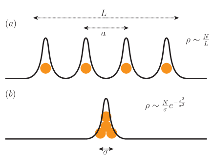
Figure 1: Initial states. $(a)$ For $\frac{a}{\sigma}\gg 1$, we have a lattice like state, $\lvert\Psi_{\text{latt}}\rangle$. $(b)$ For $a=0$, we have a condensate like state $\lvert\Psi_{\text{cond}}\rangle$, $\sigma$ determines the spread.

The quench dynamics can be studied theoretically and experimentally by observing the time evolution of physical quantities that may be local operators, multi particle observables, correlation functions, local currents or also global quantities such as entanglements. Consider an observable $\hat{A}$, it will evolve under $H$ as,

$$\langle\hat{A}(t)\rangle=\langle\psi_{0}|e^{iHt}\hat{A}e^{-iHt}|\psi_{0}\rangle.$$

To compute the evolution it is convenient to expand the initial state in the eigenbasis of the evolution Hamiltonian,

$$\lvert\Psi_{0}\rangle=\sum_{\{n\}}C_{n}\lvert n\rangle,$$ (I.1)

where $\lvert n\rangle$ are the eigenstates of $H$ and $C_{n}=\langle n\rvert\Psi_{0}\rangle$ are the overlaps with the initial state, determining the weights with which different eigenstates contribute to the time evolution:

$$\lvert\Psi_{0},t\rangle=\sum_{\{n\}}e^{-i\epsilon_{n}t}C_{n}\lvert n\rangle.$$ (I.2)

The evolution of observables is then given by,

$$\langle\hat{A}(t)\rangle_{\Psi_{0}} =\langle\Psi_{0},t|\hat{A}\lvert\Psi_{0},t\rangle=\sum_{\{n,m\}}e^{-i(\epsilon_{m}-\epsilon_{n})t}C^{*}_{n}\,C_{m}\langle n|\hat{A}\lvert m\rangle,$$ (I.3)

Many issues in dynamics and quantum kinetics revolve around expressions of this type, some already mentioned: does the system thermalize Rigol et al. (2008); Srednicki (1994); Deutsch (1991), equilibrate, cross phase transitions in time, generate defects as it evolves, what entropy is best suited to describe the evolution, what is the quantum work done in the quench. Some of these questions are discussed in other lectures of the School and we shall confine our attention to issues related to the dynamics and how to compute the evolution itself.

The quench is typically not a low energy process. A finite amount of energy (or energy per unit volume) is injected into the system,

$$\epsilon_{\text{quench}}=\langle\Psi_{0}\rvert H\lvert\Psi_{0}\rangle=\sum_{\{n\}}\epsilon_{n}\lvert C_{n}\rvert^{2},$$ (I.4)

and is conserved throughout the evolution. It specifies the energy surface on which the system moves (and the temperature, if the system thermalizes.) This surface is determined by the initial state through the overlaps $C_{n}$. Unlike the situation in thermodynamics where the ground state and low-lying excitations play a central role, this is not the case when out-of-equilibrium. A quench puts energy into the isolated system which it cannot dissipate and relax to its ground state. Rather, the eigenstates that contribute to the dynamics depend strongly on the initial state via the overlaps $C_{n}$ (see Fig. 2).

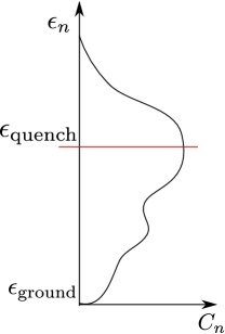
Figure 2: Difference between quench dynamics and thermodynamics. After a quench, the system probes high energy states and does not necessarily relax to the ground state. In thermodynamics, we minimize the energy (or free energy) of a system and probe the region near the ground state.

In the experiments that we seek to describe in this lecture, a system of $N$ bosons is initially confined to a region of space of size $L$ and then allowed to evolve on the infinite line while interacting with short range interactions. The quantum Hamiltonian describing the system in 1-$d$ is called the Lieb-Liniger Hamiltonian,

$$H=\int dx\,\partial b^{\dagger}(x)\partial b(x)+c\int dx\,b^{\dagger}(x)b(x)b^{\dagger}(x)b(x),$$ (I.5)

where the field $b^{\dagger}(x)$ creates a boson at point $x$. The strength and sign of the coupling constant $c$ can be controlled in the experiment. When $c>0$ the system is repulsive, whereas when $c<0$ the system is attractive and bound states appear. The choice of short range potential $V(x-y)=c\delta(x-y)$ renders the model integrable, as we shall discuss below.

Several time scales underlie the phenomena we describe. One is determined by the initial condition (spatial extent, overlap of nearby wave-functions), and the other is determined by the parameters of the quenched system (mass, interaction strength). For an extended system where we start with a locally uniform density (see Fig. 1$a$), we expect the dynamics to be in the constant density regime as long as $t\ll\frac{L}{v}$, $v$ being the characteristic velocity of propagation. Although the low energy thermodynamics of a constant density Bose gas can be described by a Luttinger liquid Giamarchi (2004), we expect the collective excitations of the quenched system to behave as a highly excited Liquid since the initial state is far from the ground state. It is also possible that depending on the energy density $\epsilon_{\text{quench}}/L$, the Luttinger liquid description may break down altogether.

The other time scale that enters the description of non equilibrium dynamics is the interaction time scale, $\tau$, a measure of the time it takes the interactions to develop fully: $\tau\sim\frac{1}{c^{2}}$ for the Lieb-Liniger model . Assuming $L$ is large enough so that $\tau\ll\frac{L}{v}$, we expect a fully interacting regime to be operative at times beyond the interactions scale until $t\sim\frac{L}{v}$ when the density of the system can no longer be considered constant. In the low density regime into which the expanding Lieb-Liniger gas enters when $t\gg\frac{L}{v}$ the effective strong coupling manifests itself as fermionization for repulsive interaction and as bound-state correlations for attractive interactions. Thus the main operation of the interaction occurs in the time range $\tau\lesssim t\lesssim\frac{L}{v}$, over which the wave function rearranges and after which the system is dilute and expands in space while interacting. In this inhomogeneous low density limit one can no longer make contact with thermodynamic ensembles, in particular, with the Generalized Gibbs ensemble Rigol et al. (2007); Calabrese and Cardy (2007); Caux and Essler (2013); Caux and Konik (2012). When $L=\infty$, the system is homogenous and free space expansion is not present. Figure 3 summarizes the different time-scales involved in a dynamical situation.

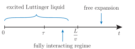
Figure 3: Time scales involved in quench dynamics. $\tau$ is an intrinsic time scale that depends on the interaction strength. $L/v$ is a characteristic time at which the system sees the finite extent.

We shall also consider initial conditions where the bosons are “condensed in space”, occupying the same single particle state characterized by some scale $\sigma$ (see Fig. 1$b$). In this case the short time dynamics is not present, the time scales at which we can measure the system are typically much larger than $\frac{\sigma}{N}$ and we expect the dynamics to be in the strongly interacting and expanding regime.

We now turn to the second term, ”integrable Hamiltonians”. It covers a vast subject which we shall address only from a particular point of view, the construction of eigenstates by means of the Bethe Ansatz. As we saw, to carry out the computation of the quench dynamics we need to know the eigenstates of the propagating Hamiltonian. The Bethe Ansatz approach is helpful in this respect as it provides us with the eigenstates of a large class of interacting one dimensional Hamiltonians. A partial list includes the Heisenberg chain (magnetism), the Hubbard model (strong-correlations), the Lieb-Liniger model and Sine-Gordon model (cold atoms in optical traps), the Kondo model and the Anderson model (impurities in metals, quantum dots) Bethe (1931); Lieb and Wu (1968); Giamarchi (2004); Lieb and Liniger (1963); Andrei et al. (1983); Andrei (1995); Tsvelick and Wiegmann (1983). Many of the Hamiltonians that can be thus be solved are of fundamental importance in condensed matter physics and have been proposed to describe various experimental situations. Integrable models pervade not only condensed matter physics but appear also in low dimensional quantum and classical field theory and statistical mechanics. They can be realized experimentally in a variety of ways and many have been extensively studied long before their integrability became manifest.

For a Hamiltonian to possess Bethe Ansatz eigenstates it must have the property that multi-particle interactions can be consistently factorized into series of two particle interactions, all of them being equivalent. Put differently, one must be able to express in a consistent way multiparticle wave functions in terms of single particle wave functions and 2-particle $S$-matrices. We shall now do so for the Lieb-Liniger Hamiltonian. The eigenstates we construct will subsequently be used to carry out quench evolution calculations in the model. The derivation of the model and its role in the description of cold atoms experiments are presented in other lectures of the School.

The Bethe Ansatz eigenstates: As the number of bosons is conserved we can consider the Hilbert space of $N$-bosons spanned by states of the form

$$|F\rangle=\int\prod_{j=1}^{N}d\,x_{j}\,F(x_{1},\cdots,x_{N})\prod_{j}b^{\dagger}(x_{j})|0\rangle,$$

with $|0\rangle$ being the vacuum state with no bosons, $b(x)|0\rangle=0$. In the $N$-boson sector, when acting on the symmetric wave function $F(x_{1},\cdots,x_{N})$, the Hamiltonian takes the form,

$$H_{N}=-\sum_{j=1}^{N}\frac{\partial^{2}}{\partial x^{2}_{j}}+2c\sum_{j<l}\delta(x_{j}-x_{l}).$$

The condition that the state $|F\rangle$ be an eigenstate of $H$ is that the wave function $F(x_{1},\cdots,x_{N})$ satisfy $H_{N}\,F=E\,F$.

We proceed to obtain the single particle wave functions and 2-particle $S$-matrices in terms of which we shall express the multiparticle wave functions. In the 1-boson sector, $H_{1}=-\frac{\partial^{2}}{\partial x^{2}}$, and the eigenstates are plane waves, $F^{\lambda}(x)=e^{i\lambda x}$, with energy $E=\lambda^{2}$. In the 2-boson sector the interaction term is present, $H_{2}=-\frac{\partial^{2}}{\partial x^{2}_{1}}-\frac{\partial^{2}}{\partial x^{2}_{2}}+2c\,\delta(x_{1}-c_{2})$. As the bosons interact only along the boundary, $x_{1}=x_{2}$, we can divide the configuration space into two regions, $x_{1}<x_{2}$ and, $x_{2}<x_{1}$ in the interior of which the particles are free and where the wave functions take the form: $Ae^{i(\lambda_{1}x_{1}+\lambda_{2}x_{2})}$ and $Be^{i(\lambda_{1}x_{1}+\lambda_{2}x_{2})}$, respectively, with energy: $E=\lambda_{1}^{2}+\lambda_{2}^{2}$. The relation between $A$ and $B$ is determined by the interaction which becomes operative on the boundary between the the two regions. The fully symmetrized wave function becomes,

$$F(x_{1},x_{2}) = \mathcal{S}e^{i(\lambda_{1}x_{1}+\lambda_{2}x_{2})}[A\theta(x_{2}-x_{1})+B\theta(x_{1}-x_{2})]=$$

$$= \;\frac{1}{2}e^{i(\lambda_{1}x_{1}+\lambda_{2}x_{2})}[A\theta(x_{2}-x_{1})+B\theta(x_{1}-x_{2})]+\frac{1}{2}e^{i(\lambda_{1}x_{2}+\lambda_{2}x_{1})}[A\theta(x_{1}-x_{2})+B\theta(x_{2}-x_{1})].$$

Here the step function $\theta(x)$ is defined as follows: $\theta(x)=1$ for $x>0$, $\theta(x)=0$ for $x<0$ and $\theta(x)=\frac{1}{2}$ for $x=0$. Hence $\theta(x)+\theta(-x)=1,\,\forall x$ and $\partial_{x}\theta(x)=\delta(x)$. Note that the wave function is continuous (as it should be) on the boundary: $F(x,x^{+})=F(x,x^{-})=\frac{1}{2}e^{i(k_{1}+k_{2})x}(A+B)$.

Applying now the Hamiltonian to the wave function, $H_{2}\,F(x_{1},x_{2})=E\,F(x_{1},x_{2})$ one finds that the condition for $F$ to be an eigenfunction is,

$$-e^{i(\lambda_{1}+\lambda_{2})x_{1}}\delta(x_{1}-x_{2})[2i\lambda_{1}(A-B)+2i\lambda_{2}(B-A)+2i\lambda_{1}(A-B)+2i\lambda_{2}(B-A)]-$$

$$-e^{i(\lambda_{1}+\lambda_{2})x_{1}}\delta^{\prime}(x_{1}-x_{2})[(A-B)+(B-A)+(A-B)+(B-A)]+$$

$$2ce^{i(\lambda_{1}+\lambda_{2})x_{1}}\delta(x_{1}-x_{2})\frac{A+B}{2}=0$$ (I.6)

The $\delta^{\prime}(x)$ term cancels automatically as result of the continuity of the wave function on the boundary. The requirement that the $\delta(x)$-terms cancel leads to the condition $B=\frac{(\lambda_{1}-\lambda_{2})+ic}{(\lambda_{1}-\lambda_{2})-ic}A$, from which we deduce the two particle $S$-matrix,

$$S^{12}=\frac{B}{A}=\frac{(\lambda_{1}-\lambda_{2})+ic}{(\lambda_{1}-\lambda_{2})-ic},$$ (I.7)

completing the determination of the two-particle eigenstate:

$$\lvert\lambda_{1}\lambda_{2}\rangle=\mathcal{N}_{12}\int_{x}Z_{12}^{x}(\lambda_{1}-\lambda_{2})e^{i(\lambda_{1}x_{1}+\lambda_{2}x_{2})}b^{\dagger}(x_{1})b^{\dagger}(x_{2})\lvert 0\rangle.$$ (I.8)

Here $\mathcal{N}_{12}$ is a normalization factor determined by a particular solution, and

$$Z^{x}_{12}(z)=\frac{z-ic\operatorname{sgn}(x_{1}-x_{2})}{z-ic}.$$ (I.9)

is the dynamic factor which includes the $S$-matrix.

The generalization to any number of particles follows a similar argument. One divides the configuration space of $N$ bosons into $N!$ regions conveniently labeled by elements $Q$ of the permutation group $S_{N}$ which specify their ordering. Thus the region where $x_{Q1}<x_{Q2}<,\cdots,x_{QN}$ corresponds to the permutation $Q$. The ordering of the particles in region $Q$ can be obtained from the ordering in some standard region, say in region $I$, where $x_{1}<x_{2},\cdots,x_{N}$, by a series of transpositions $P^{ij}$ where the positions of two adjacent particles $Qm=i,Q(m+1)=j$ are exchanged. The amplitude $A_{Q}$ in region $Q$ is given then as:

$$A_{Q}=\left(\prod S\right)\,A_{I}$$ (I.10)

where the product of $S$-matrices is taken along a path of transpositions leading from $I$ to $Q$. That path is not unique, hence for the construction to be consistent the S matrices must satisfy the condition - the Yang-Baxter equation,

$$S^{ij}S^{ik}S^{jk}=S^{jk}S^{ik}S^{ij}$$ (I.11)

guaranteeing path independence. This condition is very stringent in general, when particles carry internal degrees of freedom and the $S$ matrices do not commute. Here the condition is satisfied as the bosons have equal mass hence the individual particle momenta are conserved under scattering and the $S$-matrices are commuting phases.

The eigenstates thus take the form

$$|\vec{\lambda}\rangle=\int_{x}e^{i\vec{\lambda}\cdot\vec{x}}\sum_{Q}A_{Q}\theta(x_{Q})\prod_{j=1}^{N}b^{\dagger}(x_{j})|0\rangle$$ (I.12)

where $\int_{x}\equiv\int\prod_{j}d\,x_{j}$ and we omitted the symmetrizer since the wave function is automatically symmetrized under the integration. The eigenstates may be recast here into a more convenient form

$$\lvert\vec{\lambda}\rangle=\mathcal{N}(\vec{\lambda})\int_{x}\prod_{i<j}Z_{ij}^{x}(\lambda_{i}-\lambda_{j})\prod_{j}e^{i\lambda_{j}x_{j}}b^{\dagger}(x_{j})\lvert 0\rangle,$$ (I.13)

where $\mathcal{N}(\lambda)$ is a normalization factor determined by a particular solution. The energy eigenvalue corresponding to the eigenstate $\lvert\vec{\lambda}\rangle$ is

$$E(\vec{\lambda})=\sum_{j}\;\lambda^{2}_{j}.$$ (I.14)

The eigesntates and eigenvaues thus obtained play a different role in the study of equilibrium and non equilibrium properties of a given quantum system. To study the thermodynamic properties one must be able to enumerate and classify all eigenstates in order to construct the partition function. To achieve this, some finite volume boundary conditions (BC) are typically imposed. One may impose periodic BC to maintain translation invariance or open BC when the system has physical ends. Imposing periodic boundary conditions on the Bethe Ansatz wave functions of the LL model leads to $N$ coupled equations,

$$e^{i\lambda_{j}L}=\prod_{l}\frac{(\lambda_{j}-\lambda_{l})+ic}{(\lambda_{j}-\lambda_{l})-ic}\quad j=1,\cdots,N.$$ (I.15)

whose solutions are the allowed momentum configurations $\{\vec{\lambda}\}$ from which the full spectrum is determined via eq.(I.14). One can then identify the ground state and the low lying excitations that dominate the low-temperature physics. The analysis and classification of the solutions of the model was given by Lieb-Liniger and by Lieb Lieb and Liniger (1963). The thermodynamic partition function was then derived by summing over all energy eigenvalues with their appropriate degeneracies by Yang and Yang Yang and Yang (1969).

In the study of nonequilibrium quench dynamics, on the other hand, the main issue is the determination of the eigenstates of the propagating Hamiltonian that enter in the time evolution of a given initial state $|\psi_{0}\rangle$. This information is encoded the overlaps, $C_{n}=\langle n|\psi_{0}\rangle$, with the ground state and low lying excitation playing no special role. Given the eigenstate expansion of the initial state one needs then to resum it with the time phases, eq.(I.2), to obtain the evolved state. The overlaps, however, are not easy to evaluate due to the complicated nature of the the Bethe eigenstates and their normalization. The problem is more pronounced in the far from equilibrium quench when the state we start with suddenly finds itself far away from the eigenstates of the new Hamiltonian [see eq. (I.2)], and all the eigenstates have non-trivial weights in the time-evolution. In all but the simplest cases, the problem is non-perturbative and the existing analytical techniques are not suited for a direct application to such a situation.

When quench calculations are carried out in finite volume all the steps mentioned are involved: (i) solving the BA equation for the spectrum and the eigenstates (ii) calculation of overlaps (iii) resummation of the evolution series. If however one is interested in the physics in the infinite volume limit, one need not (unlike in thermodynamics) pass through finite volume calculation. Instead one can carry out the quench directly in the infinite volume limit allowing the the overlaps to pick out the relevant contributions. Working in the infinite volume limit allows us to replace the discrete sum in eq.(I.3) by integrations over continuous momentum variables transforming the difficult talk of computing overlaps to the simpler one, of calculaeq(ting residues in Cauchy type integrals, as we discuss below. This approach, due to V. Yudson, circumvents some of the difficulties mentioned and leads to an efficient calculational formalism and to transparent physical results. Its application to the Lieb-Liniger model is the main topic of these notes. We have applied this approach to other models too, results will be presented elsewhere.

II Time evolution on the infinite line

In 1985, V. I. Yudson presented a new approach to time evolve the Dicke model (a model for superradiance in quantum optics Dicke (1954)) considered on an infinite line Yudson (1985). The dynamics in certain cases was extracted in closed form with much less work than previously required, and in some cases where it was even impossible with earlier methods. The core of the method is to bypass the laborious sum over momenta using an appropriately chosen set of contours and integrating over momentum variables in the complex plane. It is applicable in its original form to models with a particular pole structure in the two particle $S$-matrix, and a linear spectrum. We generalize the approach to the case of the quadratic spectrum and apply it to the study of quantum quenches.

As discussed earlier, in order to carry out the quench of a system given at $t=0$ in a state $|\Psi_{0}\rangle$ one naturally proceeds by introducing a “unity” in terms of a complete set of eigenstates,

$$\lvert\Psi_{0}\rangle=\sum_{\{\lambda\}}\lvert\vec{\lambda}\rangle\langle\vec{\lambda}|\Psi_{0}\rangle$$ (II.1)

and then applies the evolution operator. The Yudson representation overcomes the difficulties in computing overlaps and carrying out this sum by using an integral representation for the (over) complete basis directly in the infinite volume limit. The argument consists of two independent parts:

1. Since the wave function for bosons, $F(x_{1},\cdots,x_{N})$, is fully symmetric it suffices to compute overlaps in a region $(x_{1}<,\cdots,<x_{N})$.

2. If no boundary conditions are imposed then the Schrodinger equation for $N$ bosons, $H\lvert\vec{\lambda}\rangle=\epsilon(\vec{\lambda})\lvert\vec{\lambda}\rangle$, is satisfied for any value of the momenta $\{\lambda_{j},j=1,\cdots,N\}$.

The initial state can then be written as

$$\lvert\Psi_{0}\rangle=\int_{\gamma}d^{N}\lambda\;C_{\vec{\lambda}}\;\lvert\vec{\lambda}\rangle$$ (II.2)

with the integration over $\vec{\lambda}$ replacing the summation over states. This is akin to summing over an over-complete basis, the relevant elements in the sum being automatically picked up by the overlap with the physical initial state. The integration over momenta will be carried out over contours $\{\gamma\}$, fixed by the pole structure of the $S$-matrices, chosen so that eq.(II.2) holds.

We proceed to carry out the evolution for the repulsive and attractive models for several initial states. The contours of integration, as we shall see, depend on the sign of the coupling constant $c$. We will notice that in the repulsive case, it is sufficient to integrate over the real line. The attractive case will require the use of contours separated out in the imaginary direction (to be qualified below). Those separated contours are consistent with the fact that the spectrum consists of “strings” with momenta taking values as complex conjugates. Actually, we shall find that the existence of string solutions (bound states) and their spectrum follow elegantly and naturally from the contour representation. They need not be known à priori, or computed from the Bethe Ansatz equations.

II.1 Repulsive interactions

We begin by discussing the repulsive case, $c>0$. For this case, a similar approach was independently developed in Ref. Tracy and Widom, 2008 and used by Lamacraft Lamacraft (2011) to calculate noise correlations in the repulsive model.

Given a generic $N$-boson initial state,

$$\lvert\Psi_{0}\rangle=\int_{\vec{x}}\Phi_{s}(\vec{x})\prod_{j}b^{{\dagger}}(x_{j})\lvert 0\rangle.$$ (II.3)

with $\Phi_{s}$ symmetrized, it can be rewritten, using the symmetry of the boson operators, in terms of basis states,

$$\lvert\Psi_{0}\rangle=N!\int_{\vec{x}}\Phi_{s}(\vec{x})\lvert\vec{x}\rangle$$ (II.4)

where,

$$\lvert\vec{x}\rangle=\theta(\vec{x})\prod_{j}b^{\dagger}(x_{j})\lvert 0\rangle.$$ (II.5)

with $\theta(\vec{x})=\theta(x_{1}>x_{2}>\cdots>x_{N})$. It suffices therefore to show that we can express any coordinate basis state as an integral over the Bethe Ansatz eigenstates,

$$\lvert\vec{x}\rangle=\theta(\vec{x})\int_{\gamma}\prod_{j}\frac{\mathrm{d}\lambda_{j}}{2\pi}A(\vec{\lambda},\vec{x})\lvert\vec{\lambda}\rangle$$ (II.6)

with appropriately chosen contours of integration $\{\gamma_{j}\}$ and $A(\lambda,\vec{x})$, which plays a role similar to the overlap of the eigenstates and the initial state. Establishing an identity of the type of eq.(II.6) corresponds to identifying the complete set of eigenstates. That is the reason that the contours for the attractive case, where bound states appear, differ from the repulsive case where they are absent.

We claim that in the repulsive case equation (II.6) is realized with

$$A(\vec{\lambda},\vec{x})=\prod_{j}e^{-i\lambda_{j}x_{j}}$$ (II.7)

and the contours $\gamma_{j}$ running along the real axis from minus to plus infinity. In other words eqn. (II.6) takes the form,

$$\lvert\vec{x}\rangle=\theta(\vec{x})\int_{\vec{y}}\int\prod_{j}\frac{{\rm d}\lambda_{j}}{2\pi}\>\prod_{i<j}Z^{y}_{ij}(\lambda_{i}-\lambda_{j})\times\prod_{j}e^{i\lambda_{j}(y_{j}-x_{j})}b^{\dagger}(y_{j})\lvert 0\rangle.$$ (II.8)

Equivalently, we claim that the $\lambda$ integration above produces $\prod_{j}\delta(y_{j}-x_{j})$.

We shall prove this in two stages. Consider first $y_{N}>x_{N}$. To carry out the integral using the residue theorem, we have to close the integration contour in $\lambda_{N}$ in the upper half plane. The poles in $\lambda_{N}$ are at $\lambda_{j}-ic$, $j<N$. These are all below $\gamma_{N}$ and so the result is zero. This implies that any non-zero contribution comes from $y_{N}\leq x_{N}$. Let us now consider $y_{N-1}>x_{N-1}$. The only pole above the contour is $\lambda_{N-1}^{*}=\lambda_{N}+ic$. However, we also have, $y_{N-1}>x_{N-1}>x_{N}\geq y_{N}\implies y_{N-1}>y_{N}$. This causes the only contributing pole to get canceled. The integral is again zero unless $y_{N-1}\leq x_{N-1}$. We can proceed is this fashion for the remaining variables thus showing that the integral is non-zero only for $y_{j}\leq x_{j}$.

Now consider $y_{1}<x_{1}$. We have to close the contour for $\lambda_{1}$ below. There are no poles in that region, and the residue is zero. Thus the integral is non-zero for only $y_{1}=x_{1}$. Consider $y_{2}<x_{2}$. The only pole below, at $\lambda_{2}^{*}=\lambda_{1}-ic$ is canceled as before since we have $y_{2}<x_{2}<x_{1}=y_{1}$. Again we get that the integral is only non-zero for $y_{2}=x_{2}$. Carrying this on, we end up with

$$\theta(\vec{x})\int_{\vec{y}}\prod_{j}\delta(y_{j}-x_{j})b^{\dagger}(y_{j})\lvert 0\rangle=\lvert\vec{x}\rangle.$$ (II.9)

In order to time evolve this state we act on it with the unitary time evolution operator. Since the integrals are well-defined we can move the operator inside the integral signs to obtain,

$$\lvert\vec{x},t\rangle=\theta(\vec{x})\int\prod_{j}\frac{{\rm d}\lambda_{j}}{2\pi}\>e^{-i\epsilon(\vec{\lambda})t}A(\vec{\lambda},\vec{x})\lvert\vec{\lambda}\rangle.$$ (II.10)

II.2 Attractive interactions

We now consider the case, $c<0$. As mentioned earlier, the spectrum of the Hamiltonian now contains complex, so-called string solutions which correspond to many-body bound states. In fact, the ground state at $T=0$ consists of one $N$-particle bound state. We will see that Yudson integral representation requires in this case another set of contours in order to establish eq.(II.6). Similar properties are seen to emerge in Prolhac and Spohn (2011), where the authors obtain a propagator for the attractive Lieb-Liniger model by analytically continuing the results obtained by Tracy and Widom Tracy and Widom (2008) for the repulsive model.

One will immediately note that for the attractive interaction the structure of the $S$-matrix is altered. This change, $c\to-c$ prevents the proof of the previous section from working. In particular, the poles in the variable $\lambda_{N}$ are at $\lambda_{j}+i\lvert c\rvert$ for $j<N$, and the residue within the contour closed in the upper half plane is not zero any more. We need choose a contour to avoid this pole. This can be achieved by separating the contours in the imaginary direction such that adjacent ${\rm Im}[\lambda_{j}-\lambda_{j-1}]>\lvert c\rvert$. At first sight, this seems to pose a problem as the quadratic term in exponent diverges at large positive $\lambda$ and positive imaginary part. There are two ways around this. We can tilt the contours as shown in Fig. 4 so that they lie in the convergent region of the Gaussian integral. The pieces towards the end, that join the real axes though essential for the proof to work at $t=0$, where we evaluate the integrals using the residue theorem, do not contribute at finite time as the integrand vanishes on them as they are taken to infinity.

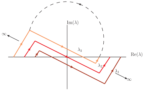
Figure 4: Contours for the $\lambda$ integration. Shown here are three contours, and the closing of the $N$th (here, third) contour as discussed in the proof.

Another more natural means of doing this is to use the finite spatial support of the initial state. The overlaps of the eigenstates with the initial state effectively restricts the support for the $\lambda$ integrals, making them convergent.

The proof of equation (II.6) now proceeds as in the repulsive case. We start by assuming that $y_{N}>x_{N}$ requiring us to close the contour in $\lambda_{N}$ in the upper half plane. This encloses no poles due to the choice of contours and the integral is zero unless $y_{N}\leq x_{N}$. Now assume $y_{N-1}>x_{N-1}$. Closing the contour above encloses one pole at $\lambda_{N-1}^{*}=\lambda_{N}-i\lvert c\rvert$, however since $y_{N-1}>x_{n-1}>x_{N}\geq y_{N}$, this pole is canceled by the numerator and again we have $y_{N-1}\leq x_{N-1}$. We proceed in this fashion and then backwards to show that the integral is non-zero only when all the poles cancel, giving us $\prod_{j}\delta(y_{j}-x_{j})$, as required.

II.3 Two particle dynamics

We begin with a detailed discussion of the quench dynamics of two bosons. As we saw, it is convenient to express any initial state in terms of an ordered coordinate basis, $\lvert\vec{x}\rangle=\theta(x_{1}>x_{2}>\cdots>x_{N})\prod_{j}b^{\dagger}(x_{j})\lvert 0\rangle$. At finite time, the wave function of bosons initially localized at $x_{1}$ and $x_{2}$ and subsequently evolved by a repulsive Lieb-Liniger Hamiltonian is given by,

$$\lvert\vec{x},t\rangle_{2} = e^{-iHt}\theta(x_{1}-x_{2})b^{\dagger}(x_{1})b^{\dagger}(x_{2})\lvert 0\rangle=$$

$$=\int_{y,\lambda}Z^{y}_{12}(\lambda_{1}-\lambda_{2})e^{-i\lambda_{1}^{2}t-i\lambda_{2}^{2}t+i\lambda_{1}(y_{1}-x_{1})+i\lambda_{2}(y_{2}-x_{2})}b^{\dagger}(y_{1})b^{\dagger}(y_{2})\lvert 0\rangle$$

$$=\int_{y}\frac{e^{i\frac{(y_{1}-x_{1})^{2}}{4t}+i\frac{(y_{2}-x_{2})^{2}}{4t}}}{4\pi it}\times\Big{[}1-c\sqrt{\pi it}\theta(y_{2}-y_{1})e^{\frac{i}{8t}\alpha^{2}}\operatorname{erfc}\left(\frac{i-1}{4}\frac{i\alpha}{\sqrt{t}}\right)\Big{]}b^{\dagger}(y_{1})b^{\dagger}(y_{2})\lvert 0\rangle$$

where $\alpha=2ct-i(y_{1}-x_{1})-i(y_{2}-x_{2})$. The above expression retains the Bethe form of wave functions defined in different configuration sectors. The only scales in the problem are the interaction strength $c$ and $x_{1}-x_{2}$, the initial separation between the particles.

In order to get physically meaningful results we need to start from a physical initial state. We choose the state $\lvert\Psi(0)_{\text{latt}}\rangle$ where bosons are trapped in a periodic trap forming initially a lattice-like state (see fig. 1a),

$$\lvert\Psi(0)_{\text{latt}}\rangle=\prod_{j}\left[\frac{1}{(\pi\sigma^{2})^{\frac{1}{4}}}\int_{\vec{x}}e^{-\frac{(x_{j}+(j-1)a)^{2}}{2\sigma^{2}}}b^{\dagger}(x_{j})\right]\lvert 0\rangle.$$ (II.12)

We shall consider two limits. The first, to which we continue to refer to as $\lvert\Psi(0)_{\text{latt}}\rangle$, is $\sigma\ll a$, with wave functions of neighboring bosons not overlapping significantly, i.e., $e^{-\frac{a^{2}}{\sigma^{2}}}\ll 1$. In this case the ordering of the initial particles needed for the Yudson representation is induced by the non-overlapping support and it becomes possible to carry out the integral analytically. The other limit, $a\ll\sigma$, when there is maximal initial overlap will be referred to as condensate (in position space) wave function $|\Psi(0)_{\text{cond}}\rangle$.

Evolution of the density: We consider the evolution of density $\hat{\rho}(x)=b^{{\dagger}}(x)b(x)$ at $x=0$ in the state $\lvert\Psi(0)_{\text{latt}}\rangle$. Fig. 5 shows $\langle\Psi_{\text{latt}},t\rvert\rho(0)\lvert\Psi_{\text{latt}},t\rangle$ for repulsive, attractive and non-interacting bosons. No difference is discernible between the three cases. The reason is obvious: the local interaction is operative only when the wave functions of the particles overlap. As we have taken $\sigma\ll a$ this will occur only after a long time when the wave-function is spread out and overlap is negligible.

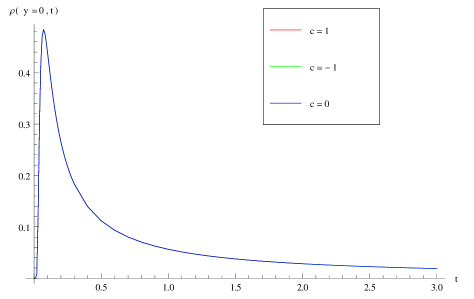
Figure 5: (Color online) $\langle\rho(x=0,t)\rangle$ vs. $t$, after the quench from $\lvert\Psi_{\text{latt}}\rangle$. $\sigma/a\sim 0.1$. The curves appear indistinguishable (i.e. lie on top of each other) since the particles start out with non significant overlap. The interaction effects would show up only when they have propagated long enough to have spread sufficiently to reach a significant overlap, at which time the density is too low.

When the separation $a$ is set to zero, with maximal initial overlap between the bosons, $|\Psi(0)_{\text{cond}}\rangle$, we expect the interaction to be operative from the start. Fig. 6 shows the density evolution for attractive, repulsive and no interaction. The decay of the density is slower for attractive model than the for the non-interacting which in turn is slower than for the repulsive model.

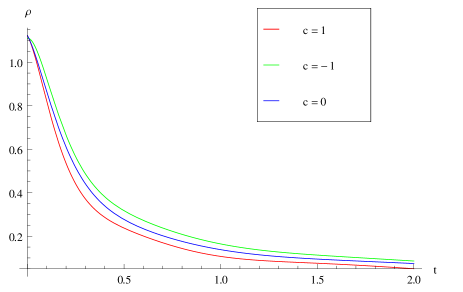
Figure 6: (Color online) $\langle\rho(x=0,t)\rangle$ vs. $t$, after the quench from $\lvert\Psi_{\text{cond}}\rangle$. $\sigma\sim 0.5,\>a=0$. As the bosons overlap interaction effects show up immediately. Lower line: $c=1$, Upper line: $c=-1$, Middle line: $c=0$.

Still, the density does not show much difference between repulsive and attractive interactions in this case. A drastic difference will appear when we study the noise correlations $\langle\Psi_{0},t|\rho(x_{1})\rho(x_{2})|\Psi_{0},t\rangle$, as will be shown below.

The appearance of bound states: Actually the apparent similarity in the behavior observed in Fig. 6 is somewhat misleading. We shall show here that for attractive interaction bound states appear in the spectrum, though their effect in evolution - in the case of two bosons - can be absorbed into the same mathematical expression as for the repulsive case.

Recall that the contours of integration are separated in the imaginary direction. In order to carry out the integration over $\lambda$, we shift the contour for $\lambda_{2}$ to the real axis, and add the residue of the pole at $\lambda_{2}=\lambda_{1}+i\lvert c\rvert$. The two particle finite time state can be written as

$$\lvert\vec{x},t\rangle_{2}=\int_{y}\int_{\gamma_{c}}\prod_{i<j=1,2}Z^{y}_{ij}(\lambda_{i}-\lambda_{j})\prod_{j=1,2}e^{-i\lambda_{j}^{2}t+i\lambda_{j}(y_{j}-x_{j})}b^{\dagger}(y_{j})\lvert 0\rangle$$ (II.13)

$$=\int_{y}\bigg{[}\int_{\gamma_{r}}\prod_{i<j,1}^{2}Z^{y}_{ij}(\lambda_{i}-\lambda_{j})\prod_{j,1}^{2}e^{-i\lambda_{j}^{2}t+i\lambda_{j}(y_{j}-x_{j})}b^{\dagger}(y_{j})\lvert 0\rangle+\theta(y_{2}-y_{1})I(\lambda_{2}=\lambda_{1}+i\lvert c\rvert,t)b^{\dagger}(y_{1})b^{\dagger}(y_{2})|0\rangle\bigg{]}$$

$\gamma_{c}$ refers to contours that are separated in imaginary direction, $\gamma_{r}$ refers to all $\lambda$ integrated along real axis. $I(\lambda_{2}=\lambda_{1}+i\lvert c\rvert,t)$ is the the residue obtained by shifting the $\lambda_{2}$ contour to the real axis from the pole at $\lambda_{2}$ at $\lambda_{1}+i\lvert c\rvert$. It is given by

$$I(\lambda_{2}=\lambda_{1}+i\lvert c\rvert,t)=-2c\int_{y}\int_{\lambda_{1}}e^{i\lambda_{1}(y_{1}-x_{1})+i(\lambda_{1}+i\lvert c\rvert)(y_{2}-x_{2})-i\lambda_{1}^{2}t-i(\lambda_{1}+i\lvert c\rvert)^{2}t}$$ (II.14)

$$=-2c\int_{y}\int_{\lambda_{1}}e^{i\lambda_{1}(y_{1}-x_{1}+y_{2}-x_{2})-\frac{\lvert c\rvert}{2}(y_{2}-y_{1})-\frac{\lvert c\rvert}{2}(x_{1}-x_{2})}e^{-i(\lambda_{1}-i\lvert c\rvert/2)^{2}t-i(\lambda_{1}+i\lvert c\rvert/2)^{2}t}$$

$$=-c\int_{y}\int_{\lambda_{1}}e^{i\lambda_{1}(y_{1}-x_{1}+y_{2}-x_{2})-\frac{\lvert c\rvert}{2}|y_{2}-y_{1}|-\frac{\lvert c\rvert}{2}(x_{1}-x_{2})}e^{-2i\lambda_{1}^{2}t+i\frac{\lvert c\rvert^{2}}{2}t}.$$

This second term corresponds to the two-particles propagating as a bound state with the wave function ($e^{-\frac{\lvert c\rvert}{2}|y_{2}-y_{1}|}$) and with center of mass position and momentum ($e^{i\lambda_{1}(y_{1}+y_{2}-x_{2}-x_{1})}$). It has a kinetic energy $2\lambda_{1}^{2}$ and a binding energy of $-c^{2}$, as reported in Yang (1968). Also the overlap of the bound state with the initial state follows immediately from the representation. It is given by $-ce^{-\frac{\lvert c\rvert}{2}(x_{1}-x_{2})}$ Such bound states appear for any number of particles involved. For instance, for three particles, the Yudson representation with complex $\lambda$’s automatically produces multiple bound-states coming from the poles, i.e. $I(\lambda_{2}=\lambda_{1}+i\lvert c\rvert)$, $I(\lambda_{3}=\lambda_{1}+i\lvert c\rvert)$, etc. They give rise to two and three particle bound states of the form $e^{-\frac{|c|}{2}(|y_{1}-y_{2}|+|y_{1}-y_{3}|+|y_{2}-y_{3}|)}$. The contribution to the above integral coming from the real axis corresponds to the non-bound state.

Finally, putting all together

$$\lvert\vec{x},t\rangle_{2}=\int_{y}\frac{e^{i\frac{(y_{1}-x_{1})^{2}}{4t}+i\frac{(y_{2}-x_{2})^{2}}{4t}}}{4\pi it}\left[1+\lvert c\rvert\sqrt{\pi it}\theta(y_{2}-y_{1})e^{\frac{i}{8t}\tilde{\alpha}^{2}}\operatorname{erfc}\left(\frac{i-1}{4}\frac{i\tilde{\alpha}}{\sqrt{t}}\right)\right]b^{\dagger}(y_{1})b^{\dagger}(y_{2})|0\rangle$$

where $\tilde{\alpha}=-2\lvert c\rvert t-i(y_{1}-x_{1})-i(y_{2}-x_{2})$. Surprisingly, the wave function maintains its form and we only need to replace $c\to-c$. This simple result is not valid for more than two particles.

Evolution of noise correlations: The density-density correlation function, $\langle\Psi_{0},t|\rho(x_{1})\rho(x_{2})|\Psi_{0},t\rangle$, involves the interaction in an essential way as the geometry of the experimental set-up measures the interference of “direct” and “crossed” propagating waves, see fig. 7a.

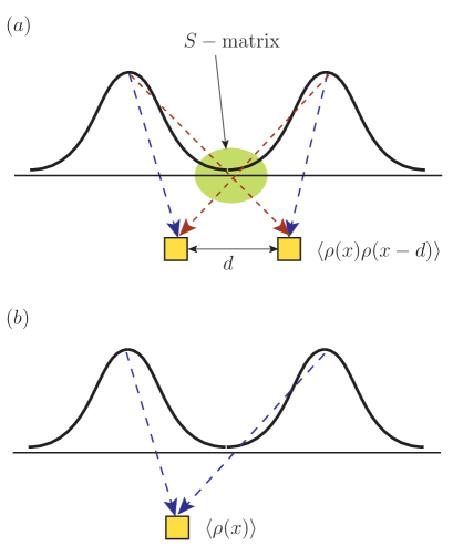
Figure 7: $(a)$ The Hanbury-Brown Twiss effect, where two detectors are used to measure the interference of the direct (big dashes) and the crossed waves (small dashes). The $S$-matrix enters explicitly. $(b)$ The density measurement is not directly sensitive to the $S$-matrix. The thick black line shows the wave-function amplitude, the dotted lines show time propagation.

The interaction among bosons is expected therefore to have a significant effect in noise measurements, more so than in density measurements which do not directly involve scattering, see fig. 7$b$.

The set-up is the famous Hanbury-Brown Twiss experiment Hanbury-Brown and Twiss (1956) where for free bosons or fermions, the crossing produces a phase of $\pm 1$ and causes destructive or constructive interference. Originally designed to study the photons arriving from two stars providing constant sources of light, in our case the set-up is generalized to multiple time dependent sources with the phase given by the two particle $S$-matrix capturing the interactions between the particles. In Fig. 8 we present the density-density correlation matrix $\langle\rho(x_{1})\rho(x_{2})\rangle$ for the repulsive gas, attractive gas, and the non-interacting gas, shown at different times, starting with the lattice initial state of two bosons. Figure 9 shows the same for the condensate initial state.

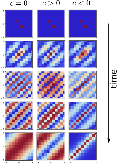
Figure 8: (Color online) Time evolution of density-density correlation matrix ($\langle\rho(x)\rho(y)\rangle$) for the $\lvert\Psi_{\text{latt}}\rangle$ initial state. Blue is zero and red is positive. The repulsive model shows anti-bunching, i.e., fermionization at long times, while the attractive model shows bunching.

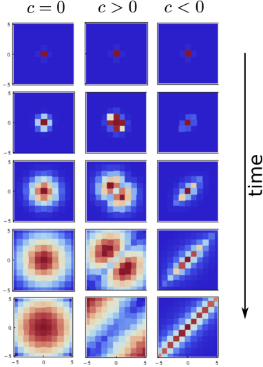
Figure 9: (Color online) Time evolution of density-density correlation matrix ($\langle\rho(x)\rho(y)\rangle$) for the $\lvert\Psi_{\text{cond}}\rangle$ initial state. Blue is zero and red is positive. The repulsive model shows anti-bunching, i.e., fermionization at long times, while the attractive model shows bunching.

In both initial states we note that the repulsive gas develops strong anti-bunching, repulsive correlations at long times akin to fermonic correlations while the attractive gas shows strong bunching correlations, enhanced bosonic in nature. We shall discuss these in detail below. We expect the results to be qualitatively similar for higher particle number, though beyond two particles the integrations cannot be carried out exactly. However, we can extract the asymptotic behavior of the wave functions analytically, as we show below.

II.4 Multiparticle dynamics at long times

Here we derive expressions for multiparticle wavefunction evolution at long times. The number of particles $N$ is kept fixed in the limiting process, hence, as discussed in the Introduction in the long time limit we are in the low density limit where interactions are expected to be dominant. The other regime where $N$ is sent to infinity first will be discussed in a separate report. We first deal with the repulsive model, for which no bound states exist and the momentum integrations can be carried out over the real line and then proceed to the attractive model. In a separate sub-section, we examine the effect of starting with a condensate-like initial state.

Repulsive interactions - quench asymptotics in the lattice state: At large time, we use the stationary phase approximation to carry out the $\lambda$ integrations. The phase oscillations come primarily from the exponent $e^{-i\lambda_{j}^{2}t+i\lambda_{j}(y_{j}-x_{j})}$. At large $t$ (i.e., $t\gg\frac{1}{c^{2}}$), the oscillations are rapid, and the stationary point is obtained by solving

$$\frac{\operatorname{d}}{\operatorname{d}\lambda_{j}}[-i\lambda_{j}^{2}t+i\lambda_{j}(y_{j}-x_{j})]=0.$$ (II.15)

Note that typically one would ignore the second term above since it doesn’t oscillate faster with increasing $t$, but here we cannot since the integral over $y$ produces a non-zero contribution for $y\sim t$ at large time. Doing the Gaussian integral around this point (and fixing the $S$-matrix prefactor to its stationary value), we obtain for the repulsive case,

$$\lvert\vec{x},t\rangle\to\int_{y}\prod_{i<j}Z^{y}_{ij}\left(\frac{y_{i}-y_{j}-x_{i}+x_{j}}{2t}\right)\prod_{j}\frac{1}{\sqrt{4\pi it}}e^{-i\frac{(y_{j}-x_{j})^{2}}{4t}+i\frac{(y_{j}-x_{j})^{2}}{2t}}b^{\dagger}(y_{j})\lvert 0\rangle.$$ (II.16)

In the above expression, the wavefunction has support mainly from regions where $y_{j}/t$ is of order one. In an experimental setup, one typically starts with a local finite density gas, i.e., a finite number of particles localized over a finite length. With this condition, at long time, we can neglect $x_{j}/t$ in comparison with $y_{j}/t$, giving

$$\lvert\vec{x},t\rangle\to\int_{y}\prod_{i<j}Z_{ij}(\xi_{i}-\xi_{j})\prod_{j}\frac{1}{\sqrt{4\pi it}}e^{it\xi_{j}^{2}-i\xi_{j}x_{j}}b^{\dagger}(y_{j})\lvert 0\rangle$$ (II.17)

where $\xi=\frac{y}{2t}$.

We turn now to calculated the asymptotic evolution of some observables. To compute the expectation value of the density we start from the coordinate basis states, $\langle\vec{x^{\prime}},t\rvert\rho(z)\lvert\vec{x},t\rangle$ which we then integrate with the chosen initial state,

$$\langle\vec{x^{\prime}},t\rvert\rho(z)\lvert\vec{x},t\rangle=\sum_{\{P\}}\int_{y}\sum_{j}\delta(y_{j}-z)\prod_{i<j}Z_{ij}(\xi_{i}-\xi_{j})Z^{*}_{P_{i}P_{j}}(\xi_{P_{i}}-\xi_{P_{j}})\prod_{j}\frac{1}{4\pi t}e^{-i(\xi_{j}x_{j}-\xi_{P_{j}}x^{\prime}_{j})}$$

Note that the above product of $S$-matrices is actually independent of the ordering of the $y$. First, only those terms appear in the product for which the permutation $P$ has an inversion. For example, say for three particles, if $P=312$, then the inversions are 13 and 23. It is only these terms which give a non-trivial $S$-matrix contribution. For the non-inverted terms, here 12, we get

$$\frac{\xi_{1}-\xi_{2}-ic\operatorname{sgn}(y_{1}-y_{2})}{\xi_{1}-\xi_{2}-ic}\frac{\xi_{1}-\xi_{2}+ic\operatorname{sgn}(y_{1}-y_{2})}{\xi_{1}-\xi_{2}+ic}$$ (II.18)

which is always unity irrespective of the ordering of $y_{1},y_{2}$. For a term with an inversion, say 23, we get,

$$\frac{\xi_{2}-\xi_{3}-ic\operatorname{sgn}(y_{2}-y_{3})}{\xi_{2}-\xi_{3}-ic}\frac{\xi_{3}-\xi_{2}+ic\operatorname{sgn}(y_{3}-y_{2})}{\xi_{3}-\xi_{2}+ic}$$ (II.19)

which is always equal to

$$\frac{\xi_{2}-\xi_{3}+ic}{\xi_{2}-\xi_{3}-ic}\equiv S(\xi_{2}-\xi_{3})$$ (II.20)

irrespective of the sign of $y_{2}-y_{3}$. This allows us to carry out the integration over the $y_{j}$.

In order to calculate physical observables, we have to choose initial states. We treat here the lattice state with $N$ particles distributed uniformly in a series of harmonic traps given by,

$$\lvert\Psi_{\text{latt}}\rangle=\int_{x}\prod_{j=1}^{N}\frac{1}{(\pi\sigma^{2})^{\frac{1}{4}}}e^{-\frac{(x_{j}+(j-1)a)^{2}}{2\sigma^{2}}}b^{\dagger}(x_{j})\lvert 0\rangle,$$ (II.21)

such that the overlap between the wave functions of two neighboring particles is negligible. In this particular case, the ordering of the particles is induced by the limited non-overlapping support of the wave function.

In this lattice-like state the initial wave function starts out with the neighboring particles having negligible overlap. At short time (as seen from (II.3)), the particle repel each other and never cross due to the repulsive interaction. So at long time, the interaction does not play a role since the wave functions are sufficiently non-overlapping. It is only the $P=1$ contribution then that survives, and we get for the density

$$\langle\vec{x}^{\prime},t\rvert\rho(z)\lvert\vec{x},t\rangle=\sum_{j}\prod_{k\neq j}\frac{\delta(x_{k}-x_{k}^{\prime})e^{-i\frac{z}{2t}(x_{j}-x_{j}^{\prime})}}{4\pi t}.$$ (II.22)

We need to integrate the position basis vectors $\lvert\vec{x}\rangle$ over some initial condition. We do this here for the lattice state (II.21) This gives

$$\rho_{\text{latt}}(\xi_{z})=\langle\Psi_{\text{latt}},t\rvert\rho(z)\lvert\Psi_{\text{latt}},t\rangle=\ \frac{N\sigma}{2\sqrt{\pi}t}e^{-\frac{\xi_{z}^{2}}{\sigma^{2}}}$$ (II.23)

Mathematically, any $S$-matrix factor that appears will necessarily have zero contribution from the pole - this is easy to see from the pole structure, and the ordering of the coordinates. In order to get a non-zero result, we need to fix at least two integration variables (i.e., the $y_{j}$). Thus the first non-trivial contribution comes from the two-point correlation function.

We now proceed to calculate the evolution of the noise, i.e., the two body correlation function

$$\rho_{2}(z,z^{\prime};t)_{\text{latt}}=\langle\Psi_{\text{latt}},t\rvert\rho(z)\rho(z^{\prime})\lvert\Psi_{\text{latt}},t\rangle$$ (II.24)

The contributions can be grouped in terms of number of crossings, which corresponds to a grouping in terms of the coefficient $e^{-ca}$ Lamacraft (2011). The leading order term can be explicitly evaluated and we show below which terms contribute. In general we have

$$\rho_{2\text{ latt}}(z,z^{\prime};t)=\sum_{\{P\}}\int_{y}\left(\sum_{j,K}\delta(y_{j}-z)\delta(y_{k}-z^{\prime})\right)\prod_{i<j,(ij)\in P}S(\xi_{i}-\xi_{j})\prod_{j}\frac{1}{4\pi t}e^{-i(\xi_{j}x_{j}-\xi_{P_{j}}x^{\prime}_{j})}.$$

The above shorthand in the $S$-matrix product means that only the $(ij)$ that belong to the inversions in $P$ are included. A detailed discussion of how to carry out the summation is given in ref. I. Here we quote the result,

$$\rho_{2\text{ latt}}(z,z^{\prime})=\frac{N^{2}\sigma^{2}}{4\pi t^{2}}e^{-(\xi_{x}^{2}+\xi_{z^{\prime}}^{2})\sigma^{2}}\bigg{[}1+\frac{2}{N^{2}}\mathrm{Re}S(\xi_{z}-\xi_{z^{\prime}})e^{ia(z-z^{\prime})}\frac{N(1-e^{ia(z-z^{\prime})}g)+e^{iaN(z-z^{\prime})}g_{zz^{\prime}}^{N}-1}{[1-g_{zz^{\prime}}e^{ia(z-z^{\prime})}]^{2}}\bigg{]}$$

where

$$g_{zz^{\prime}}=1-2c\sqrt{\pi}\sigma S(\xi_{z}-\xi_{z^{\prime}}-ic)\Big{[}e^{(c+i\xi_{z})^{2}\sigma^{2}}\operatorname{erfc}\{(c+i\xi_{z})\sigma\}+e^{(c-i\xi_{z^{\prime}})^{2}\sigma^{2}}\operatorname{erfc}\{(c-i\xi_{z^{\prime}})\sigma\}\Big{]}$$

To compare with the Hanbury-Brown Twiss result, we calculate the normalized spatial noise correlations, given by $C_{2}(z,z^{\prime})\equiv\frac{\rho_{2}(z,z^{\prime})}{\rho(z)\rho(z^{\prime})}-1$. In the non-interacting case, i.e., $c=0$, $S(\xi)=1$ and $g_{zz^{\prime}}=0$ and we recover the HBT result for $N=2$,

$$C_{2}^{0}(\xi_{z},\xi_{z^{\prime}})=\frac{1}{2}\cos(a(\xi_{z}-\xi_{z}^{\prime}))$$ (II.25)

One can also check that the limit of $c\to\infty$ gives the expected answer for free fermions, namely,

$$C_{2}^{\infty}(\xi_{z},\xi_{z^{\prime}})=-\frac{1}{2}\cos(a(\xi_{z}-\xi_{z}^{\prime}))$$ (II.26)

At finite $c$ we can see a sharp fermionic character appear that broadens with increasing $c$ as shown in Fig. 10.

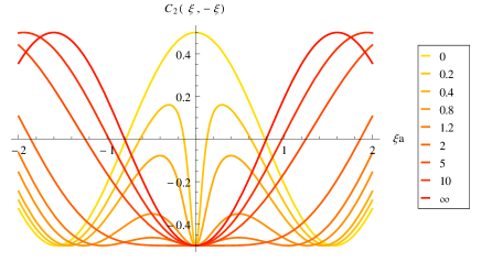
Figure 10: (Color online) Normalized noise correlation function $C_{2}(\xi,-\xi)$. Fermionic correlations develop on a time scale $\tau\sim c^{-2}$, so that for any $c$ we get a sharp fermionic peak near $\xi=0$, i.e., at large time. The key shows values of $ca$ (from Ref. Iyer and Andrei, 2012).

The large time behavior is captured in a small window around $\xi=0$. One can see that at any finite $c$, the region near zero develops a strong fermionic character, thus indicating that irrespective of the value of the coupling that we start with, the model flows towards an infinitely repulsive model at large time, that can be described in terms of free fermions. We also obtained this result “at” $t=\infty$ at the beginning of this section.

For higher particle number, we see “interference fringes” corresponding to the number of particles, that get narrower and more numerous with an increase, memory of the initial lattice state. However, the asymptotic fermionic character does not disappear. Figures 11 and 12 show the noise correlation function for five and ten particles respectively. The large peaks are interspersed by smaller peaks and so on. This reflects the character of the initial state.

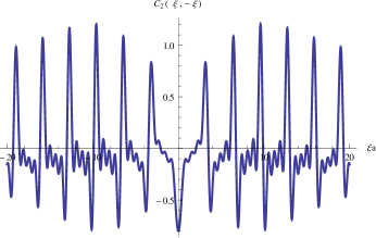
Figure 11: Normalized noise correlation function for five particles released for a Mott-like state for $c>0$ (from Ref. Iyer and Andrei, 2012)

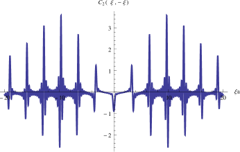
Figure 12: Normalized noise correlation function for ten particles released for a Mott-like state for $c>0$.

Attractive interactions - quench asymptotics in the lattice state: For the attractive case, since the contours of integration are spread out in the imaginary direction, we have the contributions from the poles in addition to the stationary phase contributions at large time. The stationary phase contribution is picked up on the real line, but as we move the contour, it stays pinned above the poles and we need to include the residue obtained from going around them, leading to sum over several terms.Fig. 13 shows an example of how this works.

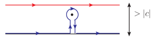
Figure 13: (Color online) Contribution from stationary phase and pole at large time in the attractive model. The blue (lower) contour represents the shifted contour.

In Ref. Iyer and Andrei, 2012, a formula was provided for the asymptotic state. Here we give a more careful treatment by taking into account that the fixed point of the approximation moves for terms that come from a pole of the $S$-matrix. It is therefore necessary to first shift the contours of integration, and then carry out the integral at long time. We carry this out below.

Shifting a contour over a pole leads to an additional term from the residue:

$$\int_{\gamma_{2}}\frac{{\rm d}\lambda_{2}}{2\pi}\to\int_{\gamma^{\rm R}_{2}}\frac{{\rm d}\lambda_{2}}{2\pi}-i\mathcal{R}(\lambda_{2}\to\lambda_{1}+i\lvert c\rvert)$$ (II.27)

where $\mathcal{R}(x)$ indicates that we evaluate the residue given by the pole $x$. $\gamma_{j}$ indicates the original contour of integration and $\gamma_{j}^{\rm R}$ indicates that integration is carried out over the real axis. Proceeding with the other variables we end up with

$$\int_{\gamma_{1},\gamma_{2},\cdots,\gamma_{N}}\to\int_{\gamma^{\rm R}_{1}}\left[\int_{\gamma^{\rm R}_{2}}+i\mathcal{R}(\lambda_{2}\to\lambda_{1}+i\lvert c\rvert)\right]\left[\int_{\gamma^{\rm R}_{3}}+i\mathcal{R}(\lambda_{3}\to\lambda_{1}+i\lvert c\rvert)+i\mathcal{R}(\lambda_{3}\to\lambda_{2}+i\lvert c\rvert)\right]\cdots\\ \times\Big{[}\int_{\gamma^{\rm R}_{N}}+i\mathcal{R}(\lambda_{N}\to\lambda_{1}+i\lvert c\rvert)+i\mathcal{R}(\lambda_{N}\to\lambda_{2}+i\lvert c\rvert)+\cdots+i\mathcal{R}(\lambda_{N}\to\lambda_{N-1}+i\lvert c\rvert)\Big{]}$$ (II.28)

The integrals can now be evaluated using the stationary phase approximation. The correction produced by the above procedure does not affect the qualitative features observed in Ref. Iyer and Andrei, 2012.

We now calculate the evolution of the density and the two body correlation function in order to compare with the repulsive case. We will first study the two particle case. Although we have a finite time expression for this case from which we can directly take a long time limit, we will study the asymptotics using the above scheme for an $N$-particle state, since we have an analytical expression to go with. We get two terms, the first being the stationary phase contribution, and is just like the repulsive case with $c\to-c$. The second is the contribution from the pole. It contains the bound state contribution which brings about another interesting feature of the attractive case. While the asymptotic dynamics of the repulsive model is solely dictated by the new variables $\xi_{j}\equiv\frac{y_{j}}{2t}$, and all the time dependence of the wave function enters through this “velocity” variable, this is not the case in the attractive model. While it is true that the system is naturally described in terms of $\xi$ variables, there still exists non-trivial time dependence.

First, we integrate out the $x$ dependence assuming an initial lattice-like state. This gives,

$$\lvert\Psi_{\text{latt}}(t)\rangle=\int_{y}\sum_{\xi_{j}^{*}=\xi_{j},\xi_{i}^{*}+ic,i<j}\prod_{i<j}S_{ij}(\xi_{i}^{*}-\xi_{j}^{*})\prod_{j}\frac{(4\pi\sigma^{2})^{\frac{1}{4}}}{\sqrt{4\pi it}}e^{-(\sigma^{2}/2+it)(\xi_{j}^{*})^{2}+i\xi_{j}^{*}(2t\xi_{j}+a(j-1))}b^{\dagger}(y_{j})\lvert 0\rangle.$$

Defining $\phi(\xi,t)$ from $\lvert\Psi_{\text{latt}}(t)\rangle=\int_{y}\phi(\xi,t)\prod_{j}b^{\dagger}(y_{j})\lvert 0\rangle$, we have for the density evolution under attractive interactions, $c<0$,

$$\rho_{\text{latt}}^{-}(z;t)=\sum_{\{P\},j}\int_{y}\delta(y_{j}-z)\phi^{*}(\xi_{P},t)\phi(\xi,t)$$ (II.29)

We can show numerically (the expressions are a bit unwieldy to write here), that asymptotically, the density shows the same Gaussian profile that we expect from a uniformly diffusing gas, namely, $e^{-\xi^{2}\sigma^{2}}$.

With this, we can proceed to compute the noise correlation function. The two particle case is easy, as there are no more integrations to carry out. We get,

$$\begin{split}\rho_{2\text{ latt}}^{-}(z,z^{\prime};t)=\sum_{\{P\},j,k}\int_{y}\delta(y_{j}-z)\delta(y_{k}-z^{\prime})\phi^{*}(\xi_{P},t)\phi(\xi,t)=\lvert\phi_{s}(\xi_{z},\xi_{z}^{\prime})\rvert^{2},\end{split}$$ (II.30)

where $\phi_{s}$ is the symmetrized wavefunction. Fig.14 shows the normalized noise correlations for different values of $t$.

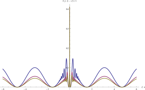
Figure 14: (Color online) Variation of $C_{2}$ for the attractive case with time. Note the growth of the central peak. At larger times, the correlations away from zero fall off. $ta^{2}=20,40,60$ for blue (top), magenta (middle) and yellow (bottom) respectively.

For more particles, we see interference fringes similar to the repulsive case. We note that the central peak increases and sharpens with time, indicating increasing contribution from bound states to the correlations (see Fig. 15 for an example).

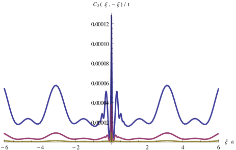
Figure 15: (Color online) $C_{2}(\xi,-\xi)$ for three particles in the attractive case plotted for three different times. At larger times, the correlations away from zero fall off. $ta^{2}=20,40,60$ for blue (top), magenta (middle) and yellow (bottom) respectively. (from Ref. Iyer and Andrei, 2012)

The condensate - attractive and repulsive interactions: We study the evolution of the Bose gas after a quench from an initial state where all the bosons are in a single level of a harmonic trap. For $t<0$, the state is described by

$$\lvert\Psi_{\text{cond}}\rangle=\int_{x}\mathcal{S}_{x}\prod_{j}\frac{e^{-\frac{x_{j}^{2}}{\sigma^{2}}}}{(\pi\sigma^{2})^{\frac{1}{4}}}b^{\dagger}(x_{j})\lvert 0\rangle.$$ (II.31)

Recall that in order to use the Yudson representation, the initial state needs to be ordered. We can rewrite the above state as

$$\lvert\Psi_{\text{cond}}\rangle=\int_{x}\mathcal{S}_{x}\theta(x_{1}>\cdots>x_{N})\prod_{j}\frac{e^{-\frac{x_{j}^{2}}{\sigma^{2}}}}{(\pi\sigma^{2})^{\frac{1}{4}}}b^{\dagger}(x_{j})\lvert 0\rangle$$ (II.32)

where $\mathcal{S}$ is a symmetrizer. The time evolution can be carried out via the Yudson representation, and again, we concentrate on the asymptotics. For the repulsive model, the stationary phase contribution is all that appears, and we get

$$\lvert\vec{x}\rangle=\int_{y}\prod_{i<j}S^{y}_{ij}\left(\frac{y_{i}-y_{j}-x_{i}+x_{j}}{2t}\right)\prod_{j}\frac{1}{\sqrt{2\pi it}}e^{-i\frac{(y_{j}-x_{j})^{2}}{4t}+i\frac{(y_{j}-x_{j})^{2}}{2t}}b^{\dagger}(y_{j})\lvert 0\rangle.$$ (II.33)

At large time $t$, we therefore have

$$\lvert\Psi_{\text{cond}}(t)\rangle=\int_{x,y}\theta(x_{1}>\cdots>x_{N})\phi_{2}(x)I(y,x,t)\prod_{j}b^{\dagger}(y_{j})\lvert 0\rangle$$ (II.34)

$\phi_{2}(x)$ is symmetric in $x$. $I(y,x,t)$ is symmetric in the $y$ but not in the $x$. Therefore we have to carry out the $x$ integration over the wedge $x_{1}>\cdots>x_{N}$. This is not straightforward to carry out. If $I(y,x,t)$ was also symmetric in $x$, then we can add the other wedges to rebuild the full space in $x$. However, due to the $S$-matrix factors, symmetrizing in $y$ does not automatically symmetrize in $x$. The exponential factors on the other hand are automatically symmetric in both variables if one of them is symmetrized because their functional dependence is of the form $f(y_{j}-x_{j})$. It is however possible to make the $S$-matrix factors approximately symmetric in $x$, and we will define what we mean by approximately shortly. What is important is to obtain a $y_{j}-x_{j}$ dependence. As of now, the $S$-matrix that appears in the above expression is

$$S^{y}_{ij}\left(\frac{y_{i}-y_{j}-x_{i}+x_{j}}{2t}\right)=\frac{\frac{y_{i}-y_{j}-x_{i}+x_{j}}{2t}-ic\operatorname{sgn}(y_{i}-y_{j})}{\frac{y_{i}-y_{j}-x_{i}+x_{j}}{2t}-ic}$$ (II.35)

First, we can change $\operatorname{sgn}(y_{i}-y_{j})$ to $\operatorname{sgn}\left(\frac{y_{i}-y_{j}}{2t}\right)$ since $t>0$. Next, note that asymptotically in time, the stationary phase contribution comes from $\frac{y}{2t}\sim\mathcal{O}(1)$. However, since $x$ has finite extent, at large enough time, $\frac{x}{2t}\sim 0$. We are therefore justified in writing $\operatorname{sgn}\left(\frac{y_{i}-x_{i}}{2t}-\frac{y_{j}-x_{j}}{2t}\right)$. The only problem could arise when $y_{i}\sim y_{j}$. However, if this occurs, then the $S$-matrix is approximately $\operatorname{sgn}(y_{i}-y_{j})$ which is antisymmetric in $ij$. With this prefactor the particles are effectively fermions, and therefore at $y_{i}\sim y_{j}$, the wave-function has an approximate node. At large time therefore, we do not have to be concerned with the possibility of particles overlapping, and including the $x_{i}$ inside the $\operatorname{sgn}$ function is valid. With this change the $S$-matrix also becomes a function of $y_{j}-x_{j}$ and symmetrizing over $y$ one automatically symmetrizes over $x$.

In short, we have established that the wave function asymptotically in time can be made symmetric in $x$. This allows us to rebuild the full space. We get

$$\lvert\Psi_{\text{cond}}(t)\rangle=\int_{x,y}\sum_{P}\theta(x_{P})\phi_{2}(x)I^{s}(y,x,t)\prod_{j}b^{\dagger}(y_{j})\lvert 0\rangle=\int_{x,y}\phi_{2}(x)I^{s}(y,x,t)\prod_{j}b^{\dagger}(y_{j})\lvert 0\rangle$$

where the $s$ superscript indicates that we have established that $I(y,x,t)$ is also symmetric in $x$. With this in mind, we can do away with the ordering when we’re integrating over the $x$ if we symmetrize the initial state wave function and the final wave function. Note that when we calculate the expectation value of a physical observable, the symmetry of the wavefunction is automatically enforced, and thus taken care of automatically.

Recall that when we calculated the noise correlations of the repulsive gas, in order to get an analytic expression for $N$ particles, we considered the leading order term, i.e., the HBT term. We did this by showing that higher order crossings produced terms higher order in $e^{-2ca}$ which we claimed was a small number. Now, however, $a=0$, and although the calculation is essentially the same with our approximate symmetrization, this simplification does not occur. The two and three particle results remain analytically calculable, but for higher numbers, we have to resort to numerical integration. Fig. 16 shows the noise correlation for two and three repulsive bosons starting from a condensate. For non-interacting particles, we expect a straight line $C_{2}=\frac{1}{2}$. When repulsive interactions are turned on, we see the characteristic fermionic dip develop. The plots for the attractive Bose gas are shown in Figs. 17 and 18. As expected from the non-interacting case the oscillations arising from the interference of particles separated spatially does not appear. The attractive however does show the oscillations near the central peak that are also visible in the case when we start from a lattice-like state. It is interesting to note that for three particles we do not see any additional structure develop in the attractive case.

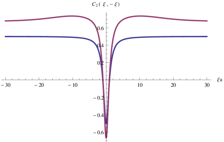
Figure 16: (Color online) $C_{2}(\xi,-\xi)$ for two (blue, bottom) and three (magenta, top)repulsive bosons starting from a condensate. Unlike the attractive case, there is no explicit time dependence asymptotically. $ca=3$ (from Ref. Iyer and Andrei, 2012)

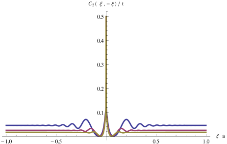
Figure 17: (Color online) Noise correlation for two attractive bosons starting from a condensate - as time increases from blue (top) to yellow (bottom), the central peak dominates.

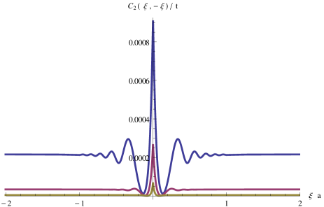
Figure 18: (Color online) $C_{2}(\xi,-\xi)$ for three attractive bosons starting from a condensate. Note that the side peak structure found in fig. 15 is missing due to the initial condition. We show the evolution at three times. As time increases, the oscillations near the central peak die out. Times from top to bottom $tc^{2}=20,40,60$. (from Ref. Iyer and Andrei, 2012)

Quenching from a bound state: In this brief section our initial state is the ground state of the attractive Lieb-Liniger Hamiltonian (with interaction strength $-c_{0}<0$. For two bosons, this take the form Lieb and Liniger (1963),

$$\lvert\Psi_{\text{bound}}\rangle=\int_{\vec{x}}e^{-c_{0}\lvert x_{1}-x_{2}\rvert-\frac{x_{1}^{2}}{2\sigma^{2}}-\frac{x_{2}^{2}}{2\sigma^{2}}}\,b^{{\dagger}}(x_{1})b^{{\dagger}}(x_{2})\lvert 0\rangle,$$ (II.36)

and we quench it with a repulsive Hamiltonian.The long time noise correlations are displayed in Fig. 19. We see that while the initial state correlations are preserved over most of the evolution, in the asymptotic long time limit the characteristic fermionic dip. We expect similar effects for any number of bosons.

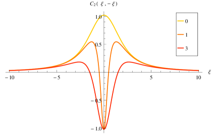
Figure 19: (Color online) Normalized noise correlation function for two particle quenched from a bound state into the repulsive regime. The legend indicates the values of $c$ that the state is quenched into. We start with $c_{0}\sigma^{2}=3,\;\sigma=1$, $c_{0}$ being the interaction strength of the initial state Hamiltonian. Again, we see the fermionic dip, but the rest of the structure is determined by the initial state.

A scaling argument We noticed the as time evolved the system developed strong correlations, enhancing the effective coupling both in the attractive and in the repulsive case. This was shown in detailed calculations of the asymptotics carried out by means of saddle point arguments. Here we proceed to show it via a simpler, though less powerful reasoning. Begin by considering repulsive interactions. From (II.6) we can see by scaling $\lambda\to\lambda\sqrt{t}$, we get $Z^{y}_{ij}(\lambda_{i}-\lambda_{j})\to\operatorname{sgn}(y_{i}-y_{j})+O\left(\frac{1}{\sqrt{t}}\right)$, yielding to leading order,

$$|\Psi_{0},t\rangle \to \int_{x}\int_{y}\int_{\lambda}\,\theta(\vec{x})\Psi_{0}(\vec{x})\prod_{j}\frac{1}{\sqrt{t}}e^{-i\lambda_{j}^{2}+i\lambda_{j}(y_{j}-x_{j})/\sqrt{t}}\prod_{i<j}\operatorname{sgn}(y_{i}-y_{j})b^{\dagger}(y_{j})\lvert 0\rangle$$ (II.37)

$$=\int_{x,y,\lambda,k}\,\theta(\vec{x})\Psi_{0}(\vec{x})\prod_{j}e^{-i\lambda_{j}^{2}t+i\lambda_{j}(y_{j}-x_{j})}e^{-ik_{j}y_{j}}c^{{\dagger}}_{k_{j}}\lvert 0\rangle$$

$$=\int_{x,k}\,\theta(\vec{x})\Psi_{0}(\vec{x})\prod_{j}e^{-ik_{j}^{2}t-ik_{j}x_{j}}c^{{\dagger}}_{k_{j}}\lvert 0\rangle$$

$$=e^{-iH^{f}_{0}t}\int_{x}\mathcal{A}_{x}\theta(\vec{x})\Psi_{0}(\vec{x})\prod_{j}c^{\dagger}(x_{j})\lvert 0\rangle,$$

with $c^{\dagger}(y)$ being fermionic creation operators replacing the hardcore bosonic operators, $\prod_{j}c^{\dagger}(y_{j})=\prod_{i<j}\operatorname{sgn}(y_{i}-y_{j})b^{\dagger}(y_{j})$. We denote $H^{f}_{0}=\int_{x}\partial c^{\dagger}(x)\partial c(x)$ the free fermionic Hamiltonian and $\mathcal{A}_{y}$ is an anti-symmetrizer acting on the $y$ variables. Thus, the repulsive Bose gas, for any value of $c>0$, is governed in the long time by the $c=\infty$ hard core boson limit (or its fermionic equivalent) Jukić et al. (2008); Girardeau (1960), and the system equilibrates (but does not thermalize) with the antisymmetric wavefunction $\tilde{\Psi}_{0}(\vec{y})=\mathcal{A}_{y}\theta(\vec{y})\Psi_{0}(\vec{y})$ and the total energy, $E_{\Psi_{0}}=\langle\Psi_{0}\rvert H\lvert\Psi_{0}\rangle$. Hence the ”fermonic” dip we observed in the noise correlation function.

For attractive interaction the argument needs to be refined since contributions of the poles have to be taken into account. They dominate in the long time limit, again corresponding to an effective increase of the attractive interaction strength as time evolves.

III Conclusions and the dynamic RG hypothesis

We have shown that the Yudson contour integral representation for arbitrary states can indeed be used to understand aspects of the quench dynamics of the Lieb-Liniger model, and obtain the asymptotic wave functions exactly. The representation overcomes some of the major difficulties involved in using the Bethe-Ansatz to study the dynamics of some integrable systems by automatically accounting for complicated states in the spectrum.

We see some interesting dynamical effects at long times. The infinite time limit of the repulsive model corresponds to particles evolving with a free fermionic Hamiltonian. It retains, however, memory of the initial state and therefore is not a thermal state. The correlation functions approach that of hard core bosons at long time indicating a dynamical increase in interaction strength. The attractive model also shows a dynamic strengthening of the interaction and the long time limit is dominated by a multiparticle bound state. This of course does not mean that it condenses. In fact the state diffuses over time, but remains strongly correlated.

We may interpret our results in terms of a “dynamic RG” in time. The asymptotic evolutions of the model both for $c>0$ and for $c<0$ are given by the Hamiltonians $H^{*}_{\pm}$ with $c\to\pm\infty$ respectively. Accepting the RG logic behind the conjecture one would expect that there would be basins of attraction around the Lieb-Liniger Hamiltonian with models whose long time evolution would bring them close to the ”dynamic fixed points” $H^{*}_{\pm}$. One such Hamiltonian would have short range potentials replacing the $\delta$-function interaction that renders the Lieb-Liniger model integrable. Perhaps, lattice models could be also found in this basin.

We have to emphasize, however, that as these models are not integrable, we do not expect that they would actually flow to $H^{*}_{\pm}$. Instead, starting close enough in the “basin”, they would flow close to $H^{*}_{\pm}$ and spend much time in its neighborhood, eventually evolving into another, thermal state. We thus conjecture that away from integrability, a system would approach the corresponding non-thermal equilibrium, where the dynamics will slow down leading to a “prethermal” state Berges et al. (2004). Fig. 20 shows a schematic of this. Such prethermalization behavior has indeed been observed in lattice models Kollath et al. (2007). The system is expected to eventually find a thermal state. It is therefore of interest to characterize different ways of breaking integrability to see when a system is “too far” from integrability to see this effect and in what regimes a system can be considered as close to integrability. For a review and background on this subject, see Ref. Polkovnikov et al., 2011.

Further, the flow diagram in Fig. 20 might have another axis that represents initial states. Studying the Bose-Hubbard model Iyer et al. (2013) shows an interesting initial state dependence. Whereas the sign of the interaction does not affect the quench dynamics, the asymptotic state depends strongly on the initial state, with a lattice-like state leading to fermionization, and a condensate-like state retaining bosonic correlations. The strong dependence on the initial state in the quench dynamics is evident from eq. (I.2) and is subject of much debate, in particular as relating to the Eigenstate Thermalization Hypothesis Rigol et al. (2008); Srednicki (1994); Deutsch (1991).

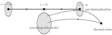
Figure 20: Schematic showing pre-thermalization of states in a non-integrable model

We showed here how to compute quantum quenches for the Lieb-Liniger model and provided predictions for experiments that can be carried out in the context of continuum cold atom systems. Application of the approach to other models is underway. This work also opens up several new questions: Though the representation is provable mathematically, further investigation is required to understand, physically, how it achieves the tedious sum over eigenstates, while automatically accounting for the details of the spectrum. It would also be useful to tie this approach to other means of calculating overlaps in the Algebraic Bethe Ansatz, i.e., the form-factor approach. The representation can essentially be thought of as a different way of writing the identity operator. From that standpoint, it could serve as a new way of evaluating correlation functions using the Bethe Ansatz.

IV Acknowledgments

We are grateful to G. Goldstein for very useful discussions. This work was supported by NSF grant DMR 1410583.

References

- Bloch et al. (2008) I. Bloch, J. Dalibard, and W. Zwerger, Rev. Mod. Phys. 80, 885 (2008).
- Moritz et al. (2003) H. Moritz, T. Stöferle, M. Köhl, and T. Esslinger, Phys. Rev. Lett. 91, 250402 (2003).
- Polkovnikov et al. (2011) A. Polkovnikov, K. Sengupta, A. Silva, and M. Vengalattore, Rev. Mod. Phys. 83, 863 (2011).
- Cazalilla et al. (2011) M. A. Cazalilla, R. Citro, T. Giamarchi, E. Orignac, and M. Rigol, Rev. Mod. Phys. 83, 1405 (2011).
- Guan et al. (2013) X.-W. Guan, M. T. Batchelor, and C. Lee, arXiv:cond-mat/1301.6446 (2013).
- Vidmar et al. (2013) L. Vidmar, S. Langer, I. McCulloch, U. Schneider, U. Schollwoeck, and F. Heidrich-Meisner, arXiv:cond-mat/1305.5496 (2013).
- Rigol et al. (2008) M. Rigol, V. Dunjko, and M. Olshanii, Nature 451, 854 (2008).
- Srednicki (1994) M. Srednicki, Phys. Rev. E 50, 888 (1994).
- Deutsch (1991) J. M. Deutsch, Phys. Rev. A 43, 2046 (1991).
- Giamarchi (2004) T. Giamarchi, Quantum Physics in One Dimension, edited by J. Birman, S. F. Edwards, R. Friend, M. Rees, D. Sherrington, and G. Veneziano, The International Series of Monographs on Physics (Oxford University Press, 2004).
- Note (1) One can refine the estimate for the interaction time setting , with . Also if we start from a lattice-like state, will include a short time scale before which the system only expands as a non-interacting gas, until neighboring wave-functions overlap sufficiently.
- Rigol et al. (2007) M. Rigol, V. Dunjko, V. Yurovsky, and M. Olshanii, Phys. Rev. Lett. 98, 050405 (2007).
- Calabrese and Cardy (2007) P. Calabrese and J. Cardy, Journal of Statistical Mechanics: Theory and Experiment 2007, P10004 (2007).
- Caux and Essler (2013) J.-S. Caux and F. H. L. Essler, (2013), arXiv:1301.3806 .
- Caux and Konik (2012) J.-S. Caux and R. M. Konik, Phys. Rev. Lett. 109, 175301 (2012).
- Bethe (1931) H. Bethe, Zeitschrift für Physik A Hadrons and Nuclei 71, 205 (1931), 10.1007/BF01341708.
- Lieb and Wu (1968) E. H. Lieb and F. Y. Wu, Phys. Rev. Lett. 20, 1445 (1968).
- Lieb and Liniger (1963) E. H. Lieb and W. Liniger, Phys. Rev. 130, 1605 (1963).
- Andrei et al. (1983) N. Andrei, K. Furuya, and J. H. Lowenstein, Rev. Mod. Phys. 55, 331 (1983).
- Andrei (1995) N. Andrei, in Low-Dimensional Quantum Field Theories for Condensed Matter Physicists: Lecture Notes of ICTP Summer Course Trieste, Italy September 1992, Series on Modern Condensed Matter Physics, Vol. 6, edited by S. Lundqvist, G. Morandi, L. Yü, and I. C. for Theoretical Physics (World Scientific, 1995).
- Tsvelick and Wiegmann (1983) A. Tsvelick and P. Wiegmann, Advances in Physics 32, 453 (1983).
- Yang and Yang (1969) C. N. Yang and C. P. Yang, Journal of Mathematical Physics 10, 1115 (1969).
- Dicke (1954) R. H. Dicke, Phys. Rev. 93, 99 (1954).
- Yudson (1985) V. I. Yudson, Soviet Physics JETP 61, 1043 (1985).
- Tracy and Widom (2008) C. A. Tracy and H. Widom, Journal of Physics A: Mathematical and Theoretical 41, 485204 (2008).
- Lamacraft (2011) A. Lamacraft, Phys. Rev. A 84, 043632 (2011).
- Prolhac and Spohn (2011) S. Prolhac and H. Spohn, Journal of Mathematical Physics 52, 122106 (2011).
- Yang (1968) C. N. Yang, Phys. Rev. 168, 1920 (1968).
- Hanbury-Brown and Twiss (1956) R. Hanbury-Brown and R. Q. Twiss, Nature 177, 27 (1956).
- Iyer and Andrei (2012) D. Iyer and N. Andrei, Phys. Rev. Lett. 109, 115304 (2012).
- Jukić et al. (2008) D. Jukić, R. Pezer, T. Gasenzer, and H. Buljan, Phys. Rev. A 78, 053602 (2008).
- Girardeau (1960) M. Girardeau, J. Math. Phys. 1, 516 (1960).
- Note (2) In spite of its similarity to the Lieb-Liniger model, the Bose-Hubbard model is not such a model. The Hamiltonian as defined on the bipartite lattice has a symmetry that leads attractive and repulsive interaction to evolve identically Iyer et al. (2013). Such a symmetry is not present in the Lieb-Liniger model. Adding to the lattice model such terms as the next nearest hopping or interactions that break this symmetry may lead to Hamiltonians in the same basin of attraction.
- Berges et al. (2004) J. Berges, S. Borsányi, and C. Wetterich, Phys. Rev. Lett. 93, 142002 (2004).
- Kollath et al. (2007) C. Kollath, A. M. Läuchli, and E. Altman, Phys. Rev. Lett. 98, 180601 (2007).
- Iyer et al. (2013) D. Iyer, H. Guan, and N. Andrei, Phys. Rev. A 87, 053628 (2013).