\copyrightdata

978-1-nnnn-nnnn-n/yy/mm

\authorinfo

Terence Parr University of San Francisco parrt@cs.usfca.edu \authorinfoJurgen Vinju Centrum Wiskunde & Informatica Jurgen.Vinju@cwi.nl

Technical Report: Towards a Universal Code Formatter through Machine Learning

(2016)

Abstract

There are many declarative frameworks that allow us to implement code formatters relatively easily for any specific language, but constructing them is cumbersome. The first problem is that “everybody” wants to format their code differently, leading to either many formatter variants or a ridiculous number of configuration options. Second, the size of each implementation scales with a language’s grammar size, leading to hundreds of rules.

In this paper, we solve the formatter construction problem using a novel approach, one that automatically derives formatters for any given language without intervention from a language expert. We introduce a code formatter called CodeBuff that uses machine learning to abstract formatting rules from a representative corpus, using a carefully designed feature set. Our experiments on Java, SQL, and ANTLR grammars show that CodeBuff is efficient, has excellent accuracy, and is grammar invariant for a given language. It also generalizes to a 4th language tested during manuscript preparation.

category:

D.2.3 Software Engineering Coding - Pretty printers

^†^†conference: SLE ’16 October 31–November 1, 2016, City, ST, Country

1 Introduction

The way source code is formatted has a significant impact on its comprehensibility MMNS83, and manually reformatting code is just not an option [mcconnel93, p.399]. Therefore, programmers need ready access to automatic code formatters or “pretty printers” in situations where formatting is messy or inconsistent. Many program generators also take advantage of code formatters to improve the quality of their output.

Because the value of a particular code formatting style is a subjective notion, often leading to heated discussions, formatters must be highly configurable. This allows, for example, current maintainers of existing code to improve their effectiveness by reformatting the code per their preferred style. There are plenty of configurable formatters for existing languages, whether in IDEs like Eclipse or standalone tools like Gnu indent, but specifying style is not easy. The emergent behavior is not always obvious, there exists interdependency between options, and the tools cannot take context information into account kooiker. For example, here are the options needed to obtain K&R C style with indent:

-nbad -bap -bbo -nbc -br -brs -c33 -cd33 -ncdb -ce
-ci4 -cli0 -cp33 -cs -d0 -di1 -nfc1 -nfca -hnl -i4
-ip0 -l75 -lp -npcs -nprs -npsl -saf -sai -saw -nsc
-nsob -nss

New languages pop into existence all the time and each one could use a formatter. Unfortunately, building a formatter is difficult and tedious. Most formatters used in practice are ad hoc, language-specific programs but there are formal approaches that yield good results with less effort. Rule-based formatting systems let programmers specify phrase-formatting pairs, such as the following sample specification for formatting the COBOL MOVE statement using ASF+SDF formatter-gen; metaenv; box; kooiker.

MOVE IdOrLit TO Id-list =
from-box( H [ "MOVE"
              H ts=25 [to-box(IdOrLit)]
              H ts=49 ["TO"]
              H ts=53 [to-box(Id-list)] ])

This rule maps a parse tree pattern to a box expression. A set of such rules, complemented with default behavior for the unspecified parts, generates a single formatter with a specific style for the given language. Section LABEL:sec:related has other related work.

There are a number of problems with rule-based formatters. First, each specification yields a formatter for one specific style. Each new style requires a change to those rules or the creation of a new set. Some systems allow the rules to be parametrized, and configured accordingly, but that leads to higher rule complexity. Second, minimal changes to the associated grammar usually require changes to the formatting rules, even if the grammar changes do not affect the language recognized. Finally, formatter specifications are big. Although most specification systems have builtin heuristics for default behavior in the absence of a specification for a given language phrase, specification size tends to grow with the grammar size. A few hundred rules are no exception.

Formatting is a problem solved in theory, but not yet in practice. Building a good code formatter is still too difficult and requires way too much work; we need a fresh approach. In this paper, we introduce a tool called CodeBuff codebuff that uses machine learning to produce a formatter entirely from a grammar for language $L$ and a representative corpus written in $L$ . There is no specification work needed from the user other than to ensure reasonable formatting consistency within the corpus. The statistical model used by CodeBuff first learns the formatting rules from the corpus, which are then applied to format other documents in the same style. Different corpora effectively result in different formatters. From a user perspective the formatter is “configured by example.”

Contributions and roadmap.

We begin by showing sample CodeBuff output in Section 2 and then explain how and why CodeBuff works in Section 3. Section LABEL:sec:evaluation provides empirical evidence that CodeBuff learns a formatting style quickly and using very few files. CodeBuff approximates the corpus style with high accuracy for the languages ANTLR, Java and SQL, and it is largely insensitive to language-preserving grammar changes. To adjust for possible selection bias and model overfitting to these three well-known languages, we tested CodeBuff on an unfamiliar language (Quorum) in Section LABEL:sec:validation, from which we learned that CodeBuff works similarly well, yet improvements are still possible. We position CodeBuff with respect to the literature on formatting in Section LABEL:sec:related_work.

2 Sample Formatting

This section contains sample SQL, Java, and ANTLR code formatted by CodeBuff, including some that are poorly formatted to give a balanced presentation. Only the formatting style matters here so we use a small font for space reasons. Github codebuff has a snapshot of all input corpora and formatted versions (corpora, testing details in Section LABEL:empirical). To arrive at the formatted output for document $d$ in corpus $D$ , our test rig removes all whitespace tokens from $d$ and then applies an instance of CodeBuff trained on the corpus without $d$ , $D\setminus\{d\}$ .

The examples are not meant to illustrate “good style.” They are simply consistent with the style of a specific corpus. In Section LABEL:sec:evaluation we define a metric to measure the success of the automated formatter in an objective and reproducible manner. No quantitative research method can capture the qualitative notion of style, so we start with these examples. (We use “…” for immaterial text removed to shorten samples.)

SQL is notoriously difficult to format, particularly for nested queries, but CodeBuff does an excellent job in most cases. For example, here is a formatted query from file IPMonVerificationMaster.sql (trained with sqlite grammar on sqlclean corpus):

SELECT DISTINCT
    t.server_name
       , t.server_id
       , ’Message Queuing Service’ AS missingmonitors
FROM t_server t INNER JOIN t_server_type_assoc tsta ON t.server_id = tsta.server_id
WHERE t.active = 1 AND tsta.type_id IN (’8’)
      AND t.environment_id = 0
      AND t.server_name NOT IN
    (
          SELECT DISTINCT l.address
          FROM ipmongroups g INNER JOIN ipmongroupmembers m ON g.groupid = m.groupid
               INNER JOIN ipmonmonitors l ON m.monitorid = l.monitorid
               INNER JOIN t_server t ON l.address = t.server_name
               INNER JOIN t_server_type_assoc tsta ON t.server_id = tsta.server_id
          WHERE l.name LIKE ’%Message Queuing Service%’
                AND t.environment_id = 0
                AND tsta.type_id IN (’8’)
                AND g.groupname IN (’Prod O/S Services’)
                AND t.active = 1
      )
UNION
ALL

And here is a complicated query from dmart_bits_IAPPBO510.sql with case statements:

SELECT
    CASE WHEN SSISInstanceID IS NULL
        THEN ’Total’
    ELSE SSISInstanceID END SSISInstanceID
    , SUM(OldStatus4) AS OldStatus4
    ...
    , SUM(OldStatus4 + Status0 + Status1 + Status2 + Status3 + Status4) AS InstanceTotal
FROM
    (
        SELECT
            CONVERT(VARCHAR, SSISInstanceID)             AS SSISInstanceID
            , COUNT(CASE WHEN Status = 4 AND
                              CONVERT(DATE, LoadReportDBEndDate) <
                              CONVERT(DATE, GETDATE())
                        THEN Status
                    ELSE NULL END)             AS OldStatus4
            ...
            , COUNT(CASE WHEN Status = 4 AND
                              DATEPART(DAY, LoadReportDBEndDate) = DATEPART(DAY, GETDATE())
                        THEN Status
                    ELSE NULL END)             AS Status4
        FROM dbo.ClientConnection
        GROUP BY SSISInstanceID
    ) AS StatusMatrix
GROUP BY SSISInstanceID

Here is a snippet from Java, our 2nd test language, taken from STLexer.java (trained with java grammar on st corpus):

switch ( c ) {
    ...
    default:
        if ( c==delimiterStopChar ) {
            consume();
            scanningInsideExpr = false;
            return newToken(RDELIM);
        }
        if ( isIDStartLetter(c) ) {
            ...
            if ( name.equals("if") ) return newToken(IF);
            else if ( name.equals("endif") ) return newToken(ENDIF);
            ...
            return id;
        }
        RecognitionException re = new NoViableAltException("", 0, 0, input);
        ...
        errMgr.lexerError(input.getSourceName(),
                          "invalid character ’"+str(c)+"’",
                          templateToken,
                          re);
        ...

Here is an example from STViz.java that indents a method declaration relative to the start of an expression rather than the first token on the previous line:

Thread t = new Thread() {
               @Override
               public void run() {
                   synchronized ( lock ) {
                       while ( viewFrame.isVisible() ) {
                           try {
                               lock.wait();
                           }
                           catch (InterruptedException e) {
                           }
                       }
                   }
               }
           };

Formatting results are generally excellent for ANTLR, our third test language. E.g., here is a snippet from Java.g4:

classOrInterfaceModifier
    :   annotation       // class or interface
    |   (   ’public’     // class or interface
            ...
        |   ’final’      // class only -- does not apply to interfaces
        |   ’strictfp’   // class or interface
        )
    ;

Among the formatted files for the three languages, there are a few regions of inoptimal or bad formatting. CodeBuff does not capture all formatting rules and occasionally gives puzzling formatting. For example, in the Java8.g4 grammar, the following rule has all elements packed onto one line (“ $\hookleftarrow$ ” means we soft-wrapped output for printing purposes):

unannClassOrInterfaceType
    :   (unannClassType_lfno_unannClassOrInterfaceType |  $\hookleftarrow$ 
unannInterfaceType_lfno_unannClassOrInterfaceType)  $\hookleftarrow$ 
(unannClassType_lf_unannClassOrInterfaceType | $\hookleftarrow$ 
unannInterfaceType_lf_unannClassOrInterfaceType)*
    ;

CodeBuff does not consider line length during training or formatting, instead mimicking the natural line breaks found among phrases of the corpus. For Java and SQL this works very well, but not always with ANTLR grammars.

Here is an interesting Java formatting issue from Compiler.java that is indented too far to the right (column 102); it is indented from the {{. That is a good decision in general, but here the left-hand side of the assignment is very long, which indents the put() code too far to be considered good style.

public ... Map<...> defaultOptionValues = new HashMap<...>() {{
                                                                  put("anchor", "true");
                                                                  put("wrap", "\n");
                                                              }};

In STGroupDir.java, the prefix token is aligned improperly:

if ( verbose ) System.out.println("loadTemplateFile("+unqualifiedFileName+") in groupdir...
                                  " prefix=" +
prefix);

We also note that some of the SQL expressions are incorrectly aligned, as in this sample from SQLQuery23.sql:

AND dmcl.ErrorMessage NOT LIKE ’%Pre-Execute phase is beginning.  %’
                               AND dmcl.ErrorMessage NOT LIKE ’%Prepare for Execute phase...
                                                              AND dmcl.ErrorMessage NOT...

Despite a few anomalies, CodeBuff generally reproduces a corpus’ style well. Now we describe the design used to achieve these results. In Section LABEL:sec:evaluation we quantify them.

3 The Design of an AI for Formatting

Our AI formatter mimics what programmers do during the act of entering code. Before entering a program symbol, a programmer decides (i) whether a space or line break is required and if line break, (ii) how far to indent the next line. Previous approaches (see Section LABEL:sec:related_work) make a language engineer define whitespace injection programmatically.

A formatting engine based upon machine learning operates in two distinct phases: training and formatting. The training phase examines a corpus of code documents, $D$ , written in language $L$ to construct a statistical model that represents the formatting style of the corpus author. The essence of training is to capture the whitespace preceding each token, $t$ , and then associate that whitespace with the phrase context surrounding $t$ . Together, the context and whitespace preceding $t$ form an exemplar. Intuitively, an exemplar captures how the corpus author formatted a specific, fine-grained piece of a phrase, such as whether the author placed a newline before or after the left curly brace in the context of a Java if-statement.

Training captures the context surrounding $t$ as an $m$ -dimensional feature vector, $X$ , that includes $t$ ’s token type, parse-tree ancestors, and many other features (Section 3.3). Training captures the whitespace preceding $t$ as the concatenation of two separate operations or directives: a whitespace $\mathit{ws}$ directive followed by a horizontal positioning $\mathit{hpos}$ directive if $\mathit{ws}$ is a newline (line break). The $\mathit{ws}$ directive generates spaces, newlines, or nothing while $\mathit{hpos}$ generates spaces to indent or align $t$ relative to a previous token (Section 3.1).

As a final step, training presents the list of exemplars to a machine learning algorithm that constructs a statistical model. There are $N$ exemplars $(X_{j},w_{j},h_{j})$ for $j=1..N$ where $N$ is the number of total tokens in all documents of corpus $D$ and $w_{j}\in\mathit{ws}$ , $h_{j}\in\mathit{hpos}$ . Machine learning models are typically both a highly-processed condensation of the exemplars and a classifier function that, in our case, classifies a context feature vector, $X$ , as needing a specific bit of whitespace. Classifier functions predict how the corpus author would format a specific context by returning a formatting directive. A model for formatting needs two classifier functions, one for predicting $\mathit{ws}$ and one for $\mathit{hpos}$ (consulted if $\mathit{ws}$ prediction yields a newline).

CodeBuff uses a $k$ -Nearest Neighbor (kNN) machine learning model, which conveniently uses the list of exemplars as the actual model. A kNN’s classifier function compares an unknown context vector $X$ to the $X_{j}$ from all $N$ exemplars and finds the $k$ nearest. Among these $k$ , the classifier predicts the formatting directive that appears most often (details in Section 3.4). It’s akin to asking a programmer how they normally format the code in a specific situation. Training requires a corpus $D$ written in $L$ , a lexer and parser for $L$ derived from grammar $G$ , and the corpus indentation size to identify indented phrases; e.g., one of the Java corpora we tested indents with 2 not 4 spaces. Let $F_{D,G}=({\bf X},W,H,\operatorname{indentSize})$ denote the formatting model contents with context vectors forming rows of matrix ${\bf X}$ and formatting directives forming elements of vectors $W$ and $H$ . Function 3 embodies the training process, constructing $F_{D,G}$ .

[] Function 1: $train$ ( $D,G,\operatorname{indentSize}$ ) $\rightarrow$ model $F_{D,G}$ X := []; $W$ := []; $H$ := []; $j$ := 1;

foreach document $d\in D$ do

tokens := tokenize(

d

);

tree := parse(tokens);

foreach $t_{i}$ $\in$ tokens do

[j]

:= compute context feature vector for

t_{i}

, tree;

W[j]

:= capture_ws(

t_{i}

);

H[j]

:= capture_hpos(

t_{i},\operatorname{indentSize}

);

j

j+1

;

end foreach

return (X, $W,H,\operatorname{indentSize}$ );

Once the model is complete, the formatting phase can begin. Formatting operates on a single document $d$ to be formatted and functions with guidance from the model. At each token $t_{i}\in d$ , formatting computes the feature vector $X_{i}$ representing the context surrounding $t_{i}$ , just like training does, but does not add $X_{i}$ to the model. Instead, the formatter presents $X_{i}$ to the $\mathit{ws}$ classifier and asks it to predict a $\mathit{ws}$ directive for $t_{i}$ based upon how similar contexts were formatted in the corpus. The formatter “executes” the directive and, if a newline, presents $X_{i}$ to the $\mathit{hpos}$ classifier to get an indentation or alignment directive. After emitting any preceding whitespace, the formatter emits the text for $t_{i}$ . Note that any token $t_{i}$ is identified by its token type, string content, and offset within a specific document, $i$ .

The greedy, “local” decisions made by the formatter give “globally” correct formatting results; selecting features for the $X$ vectors is critical to this success. Unlike typical machine learning tasks, our predictor functions do not yield trivial categories like “it’s a cat.” Instead, the predicted $\mathit{ws}$ and $\mathit{hpos}$ directives are parametrized. The following sections detail how CodeBuff captures whitespace, computes feature vectors, predicts directives, and formats documents.

3.1 Capturing whitespace as directives

In order to reproduce a particular style, formatting directives must encode the information necessary to reproduce whitespace encountered in the training corpus. There are five canonical formatting directives:

1.

$\mathit{nl}$ : Inject newline
2.

$\mathit{sp}$ : Inject space character
3.

$(\mathit{align},t)$ : Left align current token with previous token $t$
4.

$(\mathit{indent},t)$ : Indent current token from previous token $t$
5.

$\mathit{none}$ : Inject nothing, no indentation, no alignment

For simplicity and efficiency, prediction for $\mathit{nl}$ and $\mathit{sp}$ operations can be merged into a single “predict whitespace” or $\mathit{ws}$ operation and prediction of $\mathit{align}$ and $\mathit{indent}$ can be merged into a single “predict horizontal position” or $\mathit{hpos}$ operation. While the formatting directives are 2- and 3-tuples (details below), we pack the tuples into 32-bit integers for efficiency, $w$ for $\mathit{ws}$ directives and $h$ for $\mathit{hpos}$ .

[] Function 2: capture_ws( $t_{i}$ ) $\rightarrow w\in ws$ newlines := num newlines between $t_{i-1}$ and $t_{i}$ ;

if newlines $>$ 0 then return ( $\mathit{nl}$ , newlines);

;

col\Delta

t_{i}

.col - (

t_{i-1}

.col + len(text(

t_{i-1}

)));

return ( $ws,col\Delta$ );

For $ws$ operations, the formatter needs to know how many ( $n$ ) characters to inject: $\mathit{ws}\in\{(\mathit{nl},n),(\mathit{sp},n),\mathit{none}\}$ as shown in Function 3.1. For example, in the following Java fragment, the proper $ws$ directive at $\color[rgb]{0,0,1}\definecolor[named]{pgfstrokecolor}{rgb}{0,0,1}\uparrow_{\!a}$ is $(\mathit{sp},1)$ , meaning “inject 1 space,” the directive at $\color[rgb]{0,0,1}\definecolor[named]{pgfstrokecolor}{rgb}{0,0,1}\uparrow_{\!b}$ is $\mathit{none}$ , and $\color[rgb]{0,0,1}\definecolor[named]{pgfstrokecolor}{rgb}{0,0,1}\uparrow_{\!c}$ is $(\mathit{nl},1)$ , meaning “inject 1 newline.”

x 

 
  $\underset{\color[rgb]{0,0,1}\definecolor[named]{pgfstrokecolor}{rgb}{0,0,1}\uparrow_{\!a}}{\mathtt{=}}$  

 
 y $\underset{\color[rgb]{0,0,1}\definecolor[named]{pgfstrokecolor}{rgb}{0,0,1}\uparrow_{\!b}}{\mathtt{;}}$ 
 $\underset{\color[rgb]{0,0,1}\definecolor[named]{pgfstrokecolor}{rgb}{0,0,1}\uparrow_{\!c}}{\mathtt{z}}$ ++;

The $\mathit{hpos}$ directives align or indent token $t_{i}$ relative to some previous token, $t_{j}$ for $j<i$ as computed by Function 3.1. When a suitable $t_{j}$ is unavailable, there are $hpos$ directives that implicitly align or indent $t_{i}$ relative to the first token of the previous line:

$hpos\in\{(\mathit{align,t_{j}}),(\mathit{indent,t_{j}}),\mathit{align},\mathit{indent}\}$

In the following Java fragments, assuming 4-space indentation, directive $(indent,\mathtt{if})$ captures the whitespace at position $\color[rgb]{0,0,1}\definecolor[named]{pgfstrokecolor}{rgb}{0,0,1}\uparrow_{\!a}$ , $(align,\mathtt{if})$ captures $\color[rgb]{0,0,1}\definecolor[named]{pgfstrokecolor}{rgb}{0,0,1}\uparrow_{\!b}$ , and $(align,\mathtt{x})$ captures $\color[rgb]{0,0,1}\definecolor[named]{pgfstrokecolor}{rgb}{0,0,1}\uparrow_{\!c}$ .

if 

 
 ( 

 
 b 

 
 ) 

 
 {
 

 
  

 
  

 
  

 
  $\underset{\color[rgb]{0,0,1}\definecolor[named]{pgfstrokecolor}{rgb}{0,0,1}\uparrow_{\!a}}{\mathtt{z}}$ ++;
 $\underset{\color[rgb]{0,0,1}\definecolor[named]{pgfstrokecolor}{rgb}{0,0,1}\uparrow_{\!b}}{\mathtt{\}}}$

f(x,
 

 
  

 
  $\underset{\color[rgb]{0,0,1}\definecolor[named]{pgfstrokecolor}{rgb}{0,0,1}\uparrow_{\!c}}{\mathtt{y}}$ )

for (int i=0; ...
 

 
  

 
  

 
  

 
  $\underset{\color[rgb]{0,0,1}\definecolor[named]{pgfstrokecolor}{rgb}{0,0,1}\uparrow_{\!d}}{\mathtt{x}}$ =i;

At position $\color[rgb]{0,0,1}\definecolor[named]{pgfstrokecolor}{rgb}{0,0,1}\uparrow_{\!d}$ , both $(\mathit{indent},\mathtt{for})$ and $(\mathit{align},\text{`('})$ capture the formatting, but training chooses indentation over alignment directives when both are available. We experimented with the reverse choice, but found this choice better. Here, $(\mathit{align},\text{`('})$ inadvertently captures the formatting because for happens to be 3 characters.

[] Function 3: capture_hpos( $t_{i},\operatorname{indentSize}$ ) $\rightarrow h\in hpos$ ancestor := leftancestor( $t_{i}$ );

if $\exists$ ancestor w/child aligned with $t_{i}$ .col then

h_{align}

(\mathit{align},ancestor\Delta,childindex)

with smallest

ancestor\Delta~{}\&~{}childindex

;

if $\exists$ ancestor w/child at $t_{i}$ .col + $\operatorname{indentSize}$ then

h_{indent}

(\mathit{indent},ancestor\Delta,childindex)

with smallest

ancestor\Delta~{}\&~{}childindex

;

if $h_{align}$ and $h_{indent}$ not nil then

return directive with smallest $ancestor\Delta$ ;

if $h_{align}$ not nil then return $h_{align}$ ;

;

if $h_{indent}$ not nil then return $h_{indent}$ ;

;

if $t_{i}$ indented from previous line then return indent;

;

return align;

To illustrate the need for $(\mathit{indent},t_{j})$ versus plain $\mathit{indent}$ , consider the following Java method fragment where the first statement is not indented from the previous line.

public void write(String str)
 

 
  

 
  

 
  

 
 throws IOException {
 

 
  

 
  

 
  

 
  $\underset{\color[rgb]{0,0,1}\definecolor[named]{pgfstrokecolor}{rgb}{0,0,1}\uparrow_{\!\hskip 11.38109pt}}{\mathtt{int}}$  n = 0;

Directive $(indent,\mathtt{public})$ captures the indentation of int but plain $\mathit{indent}$ does not. Plain $\mathit{indent}$ would mean indenting 4 spaces from throws, the first token on the previous line, incorrectly indenting int 8 spaces relative to public.

Directive $indent$ is used to approximate nonstandard indentation as in the following fragment.

f(100,
 

 
  

 
  

 
  $\underset{\color[rgb]{0,0,1}\definecolor[named]{pgfstrokecolor}{rgb}{0,0,1}\uparrow_{\!}}{\mathtt{0}}$ );

At the indicated position, the whitespace does not represent alignment or standard 4 space indentation. As a default for any nonstandard indentation, function capture_hpos returns plain $\mathit{indent}$ as an approximation.

When no suitable alignment or indentation token is available, but the current token is aligned with the previous line, training captures the situation with directive $align$ :

return x +
 

 
  

 
  

 
  

 
 y +
 

 
  

 
  

 
  

 
 z; // align with first token of previous line

While $(align,\mathtt{y})$ is valid, that directive is not available because of limitations in how $\mathit{hpos}$ directives identify previous tokens, as discussed next.

3.2 How Directives Refer to Earlier Tokens

The manner in which training identifies previous tokens for $\mathit{hpos}$ directives is critical to successfully formatting documents and is one of the key contributions of this paper. The goal is to define a “token locator” that is as general as possible but that uses the least specific information. The more general the locator, the more previous tokens directives can identify. But, the more specific the locator, the less applicable it is in other contexts. Consider the indicated positions within the following Java fragments where $align$ directives must identify the first token of previous function arguments.

f(x,
 

 
  

 
  $\underset{\color[rgb]{0,0,1}\definecolor[named]{pgfstrokecolor}{rgb}{0,0,1}\uparrow_{\!a}}{\mathtt{y}}$ )

f(x+1,
 

 
  

 
  $\underset{\color[rgb]{0,0,1}\definecolor[named]{pgfstrokecolor}{rgb}{0,0,1}\uparrow_{\!b}}{\mathtt{y}}$ )

f(x+1,
 

 
  

 
 y,
 

 
  

 
  $\underset{\color[rgb]{0,0,1}\definecolor[named]{pgfstrokecolor}{rgb}{0,0,1}\uparrow_{\!c}}{\mathtt{-}}$ z)

The absolute token index within a document is a completely general locator but is so specific as to be inapplicable to other documents or even other positions within the same document. For example, all positions $\color[rgb]{0,0,1}\definecolor[named]{pgfstrokecolor}{rgb}{0,0,1}\uparrow_{\!a}$ , $\color[rgb]{0,0,1}\definecolor[named]{pgfstrokecolor}{rgb}{0,0,1}\uparrow_{\!b}$ , and $\color[rgb]{0,0,1}\definecolor[named]{pgfstrokecolor}{rgb}{0,0,1}\uparrow_{\!c}$ could use a single formatting directive, $(align,i)$ , but x’s absolute index, $i$ , is valid only for a function call at that specific location.

The model also cannot use a relative token index referring backwards. While still fully general, such a locator is still too specific to a particular phrase. At position $\color[rgb]{0,0,1}\definecolor[named]{pgfstrokecolor}{rgb}{0,0,1}\uparrow_{\!a}$ , token x is at delta 2, but at position $\color[rgb]{0,0,1}\definecolor[named]{pgfstrokecolor}{rgb}{0,0,1}\uparrow_{\!b}$ , x is at delta 4. Given argument expressions of arbitrary size, no single token index delta is possible and so such deltas would not be widely applicable. Because the delta values are different, the model could not use a single formatting directive to mean “align with previous argument.” The more specific the token locator, the more specific the context information in the feature vectors needs to be, which in turn, requires larger corpora (see Section 3.3).

We have designed a token locator mechanism that strikes a balance between generality and applicability. Not every previous token is reachable but the mechanism yields a single locator for x from all three positions above and has proven widely applicable in our experiments. The idea is to pop up into the parse tree and then back down to the token of interest, x, yielding a locator with two components: A path length to an ancestor node and a child index whose subtree’s leftmost leaf is the target token. This alters formatting directives relative to previous tokens to be: $(\_,ancestor\Delta,child)$ .

Unfortunately, training can make no assumptions about the structure of the provided grammar and, thus, parse-tree structure. So, training at $t_{i}$ involves climbing upwards in the tree looking for a suitable ancestor. To avoid the same issues with overly-specific elements that token indexes have, the path length is relative to what we call the earliest left ancestor as shown in the parse tree in Figure 1 for f(x+1,y,-z).

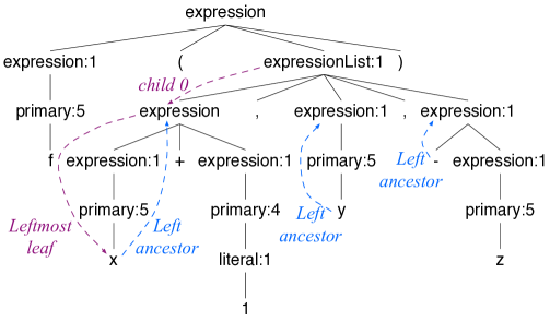
Refer to caption — Figure 1: Parse tree for f(x+1,y,-z). Node rule:n in the tree indicates the grammar rule and alternative production number used to match the subtree phrase.

The earliest left ancestor (or just left ancestor) is the oldest ancestor of $t$ whose leftmost leaf is $t$ , and identifies the largest phrase that starts with $t$ . (For the special case where $t$ has no such ancestor, we define left ancestor to be $t$ ’s parent.) It attempts to answer “what kind of thing we are looking at.” For example, the left ancestor computed from the left edge of an arbitrarily-complex expression always refers to the root of the entire expression. In this case, the left ancestors of x, y, and z are siblings, thus, normalizing leaves at three different depths to a common level. The token locator in a directive for x in f(x+1,y,-z) from both y and z is $(\_,ancestor\Delta,child)$ = $(\_,1,0)$ , meaning jump up 1 level from the left ancestor and down to the leftmost leaf of the ancestor’s child 0.

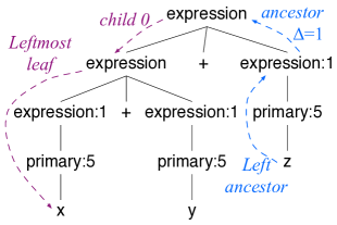
The use of the left ancestor and the ancestor’s leftmost leaf is critical because it provides a normalization factor among dissimilar parse trees about which training has no inherent structural information. Unfortunately, some tokens are unreachable using purely leftmost leaves. Consider the return x+y+z; example from the previous section and one possible parse tree for it in Figure 2. Leaf y is unreachable as part of formatting directives for z because y is not a leftmost leaf of an ancestor of z. Function capture_hpos must either align or indent relative to x or fall back on the plain $\mathit{align}$ and $\mathit{indent}$ .

The opposite situation can also occur, where a given token is unintentionally aligned with or indented from multiple tokens. In this case, training chooses the directive with the smallest $ancestor\Delta$ , with ties going to indentation.

And, finally, there could be multiple suitable tokens that share a common ancestor but with different child indexes. For example, if all arguments of f(x+1,y,-z) are aligned, the parse tree in Figure 1 shows that $(align,1,0)$ is suitable to align y and both $(align,1,0)$ and $(align,1,2)$ could align argument -z. Ideally, the formatter would align all function arguments with the same directive to reduce uncertainty in the classifier function (Section 3.4) so training chooses $(align,1,0)$ for both function arguments.

The formatting directives capture whitespace in between tokens but training must also record the context in which those directives are valid, as we discuss next.

3.3 Token Context—Feature Vectors

For each token present in the corpus, training computes an exemplar that associates a context with a $\mathit{ws}$ and $\mathit{hpos}$ formatting-directive: $(X,w,h)$ . Each context has several features combined into a $m$ -dimensional feature vector, $X$ . The context information captured by the features must be specific enough to distinguish between language phrases requiring different formatting but not so specific that classifier functions cannot recognize any contexts during formatting. The shorter the feature vector, the more situations in which each exemplar applies. Adding more features also has the potential to confuse the classifier.

Through a combination of intuition and exhaustive experimentation, we have arrived at a small set of features that perform well. There are 22 context features computed during training for each token, but $\mathit{ws}$ prediction uses only $11$ of them and $\mathit{hpos}$ uses $17$ . (The classifier function knows which subset to use.) The feature set likely characterises the context needs of the languages we tested during development to some degree, but the features appear to generalize well (Section LABEL:generalize).

Before diving into the feature details, it is worth describing how we arrived at these 21 features and how they affect formatter precision and generality. We initially thought that a sliding window of, say, four tokens would be sufficient context to make the majority of formatting decisions. For example, the context for $\cdots$ x= $\underset{\color[rgb]{0,0,1}\definecolor[named]{pgfstrokecolor}{rgb}{0,0,1}\uparrow_{\!}}{\tt 1}$ * $\cdots$ would simply be the token types of the surrounding tokens: $X$ =[id,=,int_literal,*]. The surrounding tokens provide useful but highly-specific information that does not generalize well. Upon seeing this exact sequence during formatting, the classifier function would find an exact match for $X$ in the model and predict the associated formatting directive. But, the classifier would not match context $\cdots$ x= $\underset{\color[rgb]{0,0,1}\definecolor[named]{pgfstrokecolor}{rgb}{0,0,1}\uparrow_{\!}}{\tt y}$ + $\cdots$ to the same $X$ , despite having the same formatting needs.

The more unique the context, the more specific the formatter can be. Imagine a context for token $t_{i}$ defined as the 20-token window surrounding each $t_{i}$ . Each context derived from the corpus would likely be unique and the model would hold a formatting directive specific to each token position of every file. A formatter working from this model could reproduce with high precision a very similar unknown file. The trade-off to such precision is poor generality because the model has “overfit” the training data. The classifier would likely find no exact matches for many contexts, forcing it to predict directives from poorly-matched exemplars.

Corpus	$N$ tokens	Unique $\mathit{ws}$	Unique $\mathit{hpos}$
antlr	19,692	3.0%	4.7%
java	42,032	3.9%	17.4%
java8	42,032	3.4%	7.5%
java_guava	499,029	0.8%	8.1%
sqlite	14,758	8.4%	30.8%
tsql	14,782	7.5%	17.9%

Figure 3: Percentage of unique context vectors in corpora.

To get a more general model, context vectors use at most two exact token type but lots of context information from the parse tree (details below). The parse tree provides information about the kind of phrase surrounding a token position rather than the specific tokens, which is exactly what is needed to achieve good generality. For example, rather than relying solely on the exact tokens after a = token, it is more general to capture the fact that those tokens begin an expression. A useful metric is the percentage of unique context vectors, which we counted for several corpora and show in Figure 3. Given the features described below, there are very few unique context for $\mathit{ws}$ decisions (a few %). The contexts for $\mathit{hpos}$ decisions, however, often have many more unique contexts because $\mathit{ws}$ uses 11-vectors and $\mathit{hpos}$ uses 17-vectors. E.g., our reasonably clean SQL corpus has 31% and 18% unique $\mathit{hpos}$ vectors when trained using SQLite and TSQL grammars, respectively.

For generality, the fewer unique contexts the better, as long as the formatter performs well. At the extreme, a model with just one $X$ context would perform very poorly because all exemplars would be of the form $(X,\_,\_)$ . The formatting directive appearing most often in the corpus would be the sole directive returned by the classifier function for any $X$ . The optimal model would have the fewest unique contexts but all exemplars with the same context having identical formatting directives. For our corpora, we found that a majority of unique contexts for $\mathit{ws}$ and almost all unique contexts for $\mathit{hpos}$ predict a single formatting directive, as shown in Figure 4. For example, 57.1% of the unique antlr corpus contexts are associated with just one $\mathit{ws}$ directive and 95.7% of the unique contexts predict one $\mathit{hpos}$ directive. The higher the ambiguity associated with a single context vector, the higher the uncertainty when predicting formatting decisions during formatting.

The guava corpus stands out as having very few unique contexts for $\mathit{ws}$ and among the fewest for $\mathit{hpos}$ . This gives a hint that the corpus might be much larger than necessary because the other Java corpora are much smaller and yield good formatting results. Figure LABEL:corpus-size shows the effect of corpus size on classifier error rates. The error rate flattens out after training on about 10 to 15 corpus files.

In short, few unique contexts gives an indication of the potential for generality and few ambiguous decisions gives an indication of the model’s potential for accuracy. These numbers do not tell the entire story because some contexts are used more frequently than others and those might all predict single directives. Further, a context associated with multiple directives could be 99% one specific directive.

Corpus	Ambiguous $\mathit{ws}$ directives	Ambiguous $\mathit{hpos}$ directives
antlr	42.9%	4.3%
java	29.8%	1.7%
java8	31.6%	3.2%
java_guava	23.5%	2.8%
sqlite_noisy	43.5%	5.0%
sqlite	24.8%	5.5%
tsql_noisy	40.7%	6.3%
tsql	29.3%	6.2%

Figure 4: Percentage of unique context vectors in corpora associated with

>1

formatting directive.

With this perspective in mind, we turn to the details of the individual features. The $\mathit{ws}$ and $\mathit{hpos}$ decisions use a different subset of features but we present all features computed during training together, broken into three logical subsets.

3.3.1 Token type and matching token features

At token index $i$ within each document, context feature-vector $X_{i}$ contains the following features related to previous tokens in the same document.

1.

$t_{i-1}$ , token type of previous token
2.

$t_{i}$ , token type of current token
3.

Is $t_{i-1}$ the first token on a line?
4.

Is paired token for $t_{i}$ the first on a line?
5.

Is paired token for $t_{i}$ the last on a line?

Feature #3 allows the model to distinguish between the following two different ANTLR grammar rule styles at $\color[rgb]{0,0,1}\definecolor[named]{pgfstrokecolor}{rgb}{0,0,1}\uparrow_{\!a}$ , when $t_{i}$ =DIGIT, using two different contexts.

DECIMAL 

 
 : 

 
  $\underset{\color[rgb]{0,0,1}\definecolor[named]{pgfstrokecolor}{rgb}{0,0,1}\uparrow_{\!a}}{\tt DI}$ GIT+ 

 
  $\underset{\color[rgb]{0,0,1}\definecolor[named]{pgfstrokecolor}{rgb}{0,0,1}\uparrow_{\!b}}{\tt\!\!\!;}$

DECIMAL
 

 
  

 
  

 
  

 
 : 

 
  

 
  

 
  $\underset{\color[rgb]{0,0,1}\definecolor[named]{pgfstrokecolor}{rgb}{0,0,1}\uparrow_{\!a}}{\tt DI}$ GIT+
 

 
  

 
  

 
  

 
  $\underset{\color[rgb]{0,0,1}\definecolor[named]{pgfstrokecolor}{rgb}{0,0,1}\uparrow_{\!b}}{\tt\!\!\!;}$

Exemplars for the two cases are:

( $X$ =[:, RULEREF, false, …], $w$ = $(sp,1)$ , $h$ = $\mathit{none}$ )
( $X^{\prime}$ =[:, RULEREF, true, …], $w^{\prime}$ = $(sp,3)$ , $h^{\prime}$ = $\mathit{none}$ )

where RULEREF is $type({\tt DIGIT})$ , the token type of rule reference DIGIT from the ANTLR meta-grammar. Without feature #3, there would be a single context associated with two different formatting directives.

Features #4 and #5 yield different contexts for common situations related to paired symbols, such as { and }, that require different formatting. For example, at position $\color[rgb]{0,0,1}\definecolor[named]{pgfstrokecolor}{rgb}{0,0,1}\uparrow_{\!b}$ , the model knows that : is the paired previous symbol for ; (details below) and distinguishes between the styles. On the left, : is not the first token on a line whereas : does start the line for the case on the right, giving two different exemplars:

( $X$ =[…, false, false], $w$ = $(sp,1)$ , $h$ = $\mathit{none}$ )
( $X^{\prime}$ =[…, true, false], $w^{\prime}$ = $(nl,1)$ , $h^{\prime}$ =( $\mathit{align}$ ,:))

Those features also allow the model to distinguish between the first two following Java cases where the paired symbol for } is sometimes not at the end of the line in short methods.

void reset() {x=0;}

void reset() {
    x=0;
}

void reset() {
    x=0;}

Without features #4-#5, the formatter would yield the third.

Determining the set of paired symbols is nontrivial, given that the training can make no assumptions about the language it is formatting. We designed an algorithm, pairs in Function 3.3.1, that analyzes the parse trees for all documents in the corpus and computes plausible token pairs for every non-leaf node (grammar rule production) encountered. The algorithm relies on the idea that paired tokens are token literals, occur as siblings, and are not repeated siblings. Grammar authors also do not split paired token references across productions. Instead, authors write productions such as these ANTLR rules for Java:

expr : ID ’[’ expr ’]’ | ... ;
type : ID ’<’ ID (’,’ ID)* ’>’ | ... ;

that yield subtrees with the square and angle brackets as direct children of the relevant production. Repeated tokens are not plausible pair elements so the commas in a generic Java type list, as in T<A,B,C>, would not appear in pairs associated with rule type. A single subtree in the corpus with repeated commas as children of a type node would remove comma from all pairs associated with rule type. Further details are available in Function 3.3.1 (source CollectTokenPairs.java). The algorithm neatly identifies pairs such as (?, :) and ([, ]), and ((, )) for Java expressions and (enum, }), (enum, {), and ({, }) for enumerated type declarations. During formatting, paired (Function 3.3.1) returns the paired symbols for $t_{i}$ .

[] Function 4: $pairs$ (Corpus $D$ ) $\rightarrow$ map node $\mapsto$ set<( $s,t$ )> pairs := map of node $\mapsto$ set<tuples>;

repeats := map of node

\mapsto

set<token types>;

foreach $d\in D$ do

foreach non-leaf node $r$ in parse( $d$ ) do

literals :=

\{t\mid parent(t)=r,t\text{ is literal token}\}

;

add

\{(t_{i},t_{j})\mid i<j\,\forall\,t_{i},t_{j}\in literals\}

to pairs[

r

];

add

\{t_{i}\mid\exists\,t_{i}=t_{j},i\neq{}j\}

to repeats[

r

];

end foreach

delete pair

(t_{i},t_{j})\in pairs[r]

t_{i}\text{ or }t_{j}\in repeats[r]\,\forall\,r

;

return pairs;

[] Function 5: $paired$ (pairs, token $t_{i}$ ) $\rightarrow$ $t^{\prime}$ mypairs := pairs[ $parent(t)$ ];

viable :=

\{s\mid(s,t)\in{\textit{m}ypairs},s\in{\textit{s}iblings}(t)\}

;

if $|$ viable $|=1$ then ttype := viable[0];

;

else if $\exists(s,t)|~{}s,t$ are common pairs then ttype :=

s

;

else if $\exists(s,t)|~{}s,t$ are single-char literals then ttype :=

s

;

else ttype := viable[0]; // choose first if still ambiguous
;

matching :=

[t_{j}\mid t_{j}=ttype,j<i,\,\forall\,t_{j}\in{\textit{s}iblings}(t_{i})]

;

return last(matching);

3.3.2 List membership features

Most computer languages have lists of repeated elements separated or terminated by a token literal, such as statement lists, formal parameter lists, and table column lists. The next group of features indicates whether $t_{i}$ is a component of a list construct and whether or not that list is split across multiple lines (“oversize”).

6.

Is $\mathit{leftancestor}(t_{i})$ a component of an oversize list?
7.

$\mathit{leftancestor}(t_{i})$ component type within list from
{prefix token, first member, first separator, member,
separator, suffix token}

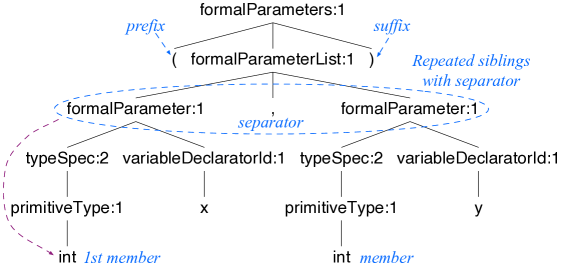
With these two features, context vectors capture not only two different overall styles for short and oversize lists but how the various elements are formatted within those two kinds of lists. Here is a sample oversize Java formal parameter list annotated with list component types:

Only the first member of a list is differentiated; all other members are labeled as just plain members because their formatting is typically the same. The exemplars would be:

( $X$ =[…, true, prefix], $w$ = $\mathit{none}$ , $h$ = $\mathit{none}$ )
( $X$ =[…, true, first member], $w$ = $\mathit{none}$ , $h$ = $\mathit{none}$ )
( $X$ =[…, true, first separator], $w$ = $\mathit{none}$ , $h$ = $\mathit{none}$ )
( $X$ =[…, true, member], $w$ = $(\mathit{nl},1)$ , $h$ = $(\mathit{align},\text{first arg})$ )
( $X$ =[…, true, separator], $w$ = $\mathit{none}$ , $h$ = $\mathit{none}$ )
( $X$ =[…, true, member], $w$ = $(\mathit{nl},1)$ , $h$ = $(\mathit{align},\text{first arg})$ )
( $X$ =[…, true, suffix], $w$ = $\mathit{none}$ , $h$ = $\mathit{none}$ )

Even for short lists on one line, being able to differentiate between list components lets training capture different but equally valid styles. For example, some ANTLR grammar authors write short parenthesized subrules like (ID|INT|FLOAT) but some write (ID | INT | FLOAT).

As with identifying token pairs, CodeBuff must identify the constituent components of lists without making assumptions about grammars that hinder generalization. The intuition is that lists are repeated sibling subtrees with a single token literal between the 1st and 2nd repeated sibling, as shown in Figure 5. Repeated subtrees without separators are not considered lists. Training performs a preprocessing pass over the parse tree for each document, tagging the tokens identified as list components with values for features #6- #7. Tokens starting list members are identified as the leftmost leaves of repeated siblings (formalParameter in Figure 5). Prefix and suffix components are the tokens immediately to the left and right of list members but only if they share a common parent.

The training preprocessing pass also collects statistics about the distribution of list text lengths (without whitespace) of regular and oversize lists. Regular and oversize list lengths are tracked per $(r,c,sep)$ combination for rule subtree root type $r$ , child node type $c$ , and separator token type $sep$ ; e.g., $(r,c,sep)$ = $($ formalParameterList, formalParameter,‘,’ $)$ in Figure 5. The separator is part of the tuple so that expressions can distinguish between different operators such as = and *. Children of binary and ternary operator subtrees satisfy the conditions for being a list, with the operator as separator token(s). For each $(r,c,sep)$ combination, training tracks the number of those lists and the median list length, $(r,c,sep)\mapsto(n,median)$ .

3.3.3 Identifying oversize lists during formatting

As with training, the formatter performs a preprocessing pass to identify the tokens of list phrases. Whereas training identifies oversize lists simply as those split across lines, formatting sees documents with all whitespace squeezed out. For each $(r,c,sep)$ encountered during the preprocessing pass, the formatter consults a mini-classifier to predict whether that list is oversize or not based upon the list string length, $ll$ . The mini-classifier compares the mean-squared-distance of $ll$ to the median for regular lists and the median for oversize (big) lists and then adjusts those distances according to the likelihood of regular vs oversize lists. The a priori likelihood that a list is regular is $p(reg)=n_{reg}/(n_{reg}+n_{big})$ , giving an adjusted distance to the regular type list as: $dist_{reg}=(ll-median_{reg})^{2}*(1-p(reg))$ . The distance for oversize lists is analogous.

When a list length is somewhere between the two medians, the relative likelihoods of occurrence shift the balance. When there are roughly equal numbers of regular and oversize lists, the likelihood term effectively drops out, giving just mean-squared-distance as the mini-classifier criterion. At the extreme, when all $(r,c,sep)$ lists are big, $p(big)=1$ , forcing $dist_{big}$ to 0 and, thus, always predicting oversize.

When a single token $t_{i}$ is a member of multiple lists, training and formatting associate $t_{i}$ with the longest list subphrase because that yields the best formatting, as evaluated manually across the corpora. For example, the expressions within a Java function call argument list are often themselves lists. In f( $e_{1}$ ,...,a+b), token a is both a sibling of f’s argument list but also the first sibling of expression a+b, which is also a list. Training and formatting identify a as being part of the larger argument list rather than the smaller a+b. This choice ensures that oversize lists are properly split. Consider the opposite choice where a is associated with list a+b. In an oversize argument list, the formatter would not inject a newline before a, yielding poor results:

f( $e_{1}$ ,
  ..., a+b)

Because list membership identification occurs in a top-down parse-tree pass, associating tokens with the largest construct is a matter of latching the first list association discovered.

3.3.4 Parse-tree context features

The final features provide parse-tree context information:

8.

$\mathit{childindex}(t_{i})$
9.

$\mathit{rightancestor}(t_{i-1})$
10.

$\mathit{leftancestor}(t_{i})$
11.

$\mathit{childindex}(\mathit{leftancestor}(t_{i}))$
12.

$\mathit{parent}_{1}(\mathit{leftancestor}(t_{i}))$
13.

$\mathit{childindex}(parent_{1}(\mathit{leftancestor}(t_{i})))$
14.

$\mathit{parent}_{2}(\mathit{leftancestor}(t_{i}))$
15.

$\mathit{childindex}(\mathit{parent}_{2}(\mathit{leftancestor}(t_{i})))$
16.

$\mathit{parent}_{3}(\mathit{leftancestor}(t_{i}))$
17.

$\mathit{childindex}(\mathit{parent}_{3}(\mathit{leftancestor}(t_{i})))$
18.

$\mathit{parent}_{4}(\mathit{leftancestor}(t_{i}))$
19.

$\mathit{childindex}(\mathit{parent}_{4}(\mathit{leftancestor}(t_{i})))$
20.

$\mathit{parent}_{5}(\mathit{leftancestor}(t_{i}))$
21.

$\mathit{childindex}(\mathit{parent}_{5}(\mathit{leftancestor}(t_{i})))$

Here the $\mathit{childindex}(p)$ is the 0-based index of node $p$ among children of $parent(p)$ , $\mathit{childindex}(t_{i})$ is shorthand for $\mathit{childindex}(\mathit{leaf}(t_{i}))$ , and $\mathit{leaf}(t_{i})$ is the leaf node associated with $t_{i}$ . Function $\mathit{childindex}(p)$ has a special case when $p$ is a repeated sibling. If $p$ is the first element, $\mathit{childindex}(p)$ is the actual child index of $p$ within the children of $\mathit{parent}(p)$ but is special marker * for all other repeated siblings. The purpose is to avoided over-specializing the context vectors to improve generality. These features also use function $\mathit{parent}_{i}(p)$ , which is the $i^{th}$ parent of $p$ ; $\mathit{parent}_{1}(p)$ is synonymous with the direct parent $parent(p)$ .

The child index of $t_{i}$ , feature #8, gives the necessary context information to distinguish the alignment token between the following two ANTLR lexical rules at the semicolon.

BooleanLiteral
    :   ’true’
    |   ’false’
    ;

fragment
DIGIT
    :   [0-9]
    ;

On the left, the ; token is child index 3 but 4 on the right, yielding different contexts, $X$ and $X^{\prime}$ , to support different alignment directives for the two cases. Training collects exemplars $(X,(\mathit{align},0,1))$ and $(X^{\prime},(\mathit{align},0,2))$ , which aligns ; with the colon in both cases.

Next, features $\mathit{rightancestor}(t_{i-1})$ and $\mathit{leftancestor}(t_{i})$ describe what phrase precedes $t_{i}$ and what phrase $t_{i}$ starts. The $\mathit{rightancestor}$ is analogous to $\mathit{leftancestor}$ and is the oldest ancestor of $t_{i}$ whose rightmost leaf is $t_{i}$ (or $\mathit{parent}(t_{i})$ if there is no such ancestor). For example, at $t_{i}$ =y in x=1; y=2; the right ancestor of $t_{i-1}$ and the left ancestor of $t_{i}$ are both “statement” subtree roots.

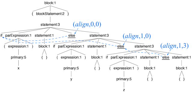
Finally, the parent and child index features capture context information about highly nested constructs, such as:

if ( x ) { }
else if ( y ) { }
else if ( z ) { }
else { }

Each else token requires a different formatting directive for alignment, as shown in Figure 6; e.g., $(\mathit{align},1,3)$ means “jump up 1 level from $\mathit{leftancestor}(t_{i})$ and align with leftmost leaf of child 3 (token else).” To distinguish the cases, the context vectors must be different. Therefore, training collects these partial vectors with features #10-15:

$X$ =[…, stat, 0, blockStat, *, block, 0, …]
$X$ =[…, stat, *, stat, 0, blockStat, *, …]
$X$ =[…, stat, *, stat, *, stat, 0, …]

where stat abbreviates statement:3 and blockStat abbreviates blockStatement:2. All deeper else clauses also use directive $(\mathit{align},1,3)$ .

Training is complete once the software has computed an exemplar for each token in all corpus files. The formatting model is the collection of those exemplars and an associated classifier that predicts directives given a feature vector.

3.4 Predicting Formatting Directives

CodeBuff’s kNN classifier uses a fixed $k=11$ (chosen experimentally in Section LABEL:empirical) and an $L_{0}$ distance function (ratio of number of components that differ to vector length) but with a twist on classic kNN that accentuates feature vector distances in a nonlinear fashion. To make predictions, a classic kNN classifier computes the distance from unknown feature vector $X$ to every $X_{j}$ vector in the exemplars, $({\bf X},Y)$ , and predicts the category, $y$ , occurring most frequently among the $k$ exemplars nearest $X$ .

The classic approach works very well in Euclidean space with quantitative feature vectors but not so well with an $L_{0}$ distance that measures how similar two code-phrase contexts are. As the $L_{0}$ distance increases, the similarity of two context vectors drops off dramatically. Changing even one feature, such as earliest left ancestor (kind of phrase), can mean very different contexts. This quick drop off matters when counting votes within the $k$ nearest $X_{j}$ . At the extreme, there could be one exemplar where $X=X_{j}$ at distance 0 and 10 exemplars at distance 1.0, the maximum distance. Clearly the one exact match should outweigh 10 that do not match at all, but a classic kNN uses a simple unweighted count of exemplars per category (10 out of 11 in this case). Instead of counting the number of exemplars per category, our variation sums $1-\sqrt[3]{L_{0}(X,X_{j})}$ for each $X_{j}$ per category. Because distances are in $[0..1]$ , the cube root nonlinearly accentuates differences. Distances of 0 count as weight 1, like the classic kNN, but distances close to 1.0 count very little towards their associated category. In practice, we found feature vectors more distant than about 15% from unknown $X$ to be too dissimilar to count. Exemplars at distances above this threshold are discarded while collecting the $k$ nearest neighbors.

The classfier function uses features #1-#10, #12 to make $\mathit{ws}$ predictions and #2, #6-#21 for $\mathit{hpos}$ ; $\mathit{hpos}$ predictions ignore $X_{j}$ not associated with tokens starting a line.

3.5 Formatting a Document

To format document $d$ , the formatter Function LABEL:format first squeezes out all whitespace tokens and line/column information from the tokens of $d$ and then iterates through $d$ ’s remaining tokens, deciding what whitespace to inject before each token. At each token, the formatter computes a feature vector for that context and asks the model to predict a formatting directive (whereas training examines the whitespace to determine the directive). The formatter uses the information in the formatting directive to compute the number of newline and space characters to inject. The formatter treats the directives like bytecode instructions for a simple virtual machine: { $(\mathit{nl},n)$ , $(\mathit{sp},n)$ , $\mathit{none}$ , $(\mathit{align,ancestor\Delta,child})$ , $(\mathit{indent,ancestor\Delta,child})$ , $\mathit{align}$ , $\mathit{indent}$ }.

As the formatter emits tokens and injects whitespace, it tracks line and column information so that it can annotate tokens with this information. Computing features #3-5 at token $t_{i}$ relies on line and column information for $t_{j}$ for some $j<i$ . For example, feature #3 answers whether $t_{i-1}$ is the first token on the line, which requires line and column information for $t_{i-1}$ and $t_{i-2}$ . Because of this, predicting the whitespace preceding token $t_{i}$ is a (fast) function of the actions made previously by the formatter. After processing $t_{i}$ , the file is formatted up to and including $t_{i}$ .

Before emitting whitespace in front of token $t_{i}$ , the formatter emits any comments found in the source code. (The ANTLR parser has comments available on a “hidden channel”.) To get the best output, the formatter needs whitespace in front of comments and this is the one case where the formatter looks at the original file’s whitespace. Otherwise, the formatter computes all whitespace generated in between tokens. To ensure single-line comments are followed by a newline, users of CodeBuff can specify the token type for single-line comments as a failsafe.

[] Function 6: format( $F_{D,G}=({\bf X},W,H,\operatorname{indentSize}),d$ ) line := col := 0;

d

d

with whitespace tokens, line/column info removed;

foreach $t_{i}\in d$ do

emit any comments to left of

t_{i}

;

X_{i}

:= compute context feature vector at

t_{i}

;

ws

:= predict directive using

X_{i}

and X,

W

;

newlines := sp := 0;