Constraining stochastic gravitational wave background from weak lensing of CMB B-modes

Abstract

A stochastic gravitational wave background (SGWB) will affect the CMB anisotropies via weak lensing. Unlike weak lensing due to large scale structure which only deflects photon trajectories, a SGWB has an additional effect of rotating the polarization vector along the trajectory. We study the relative importance of these two effects, deflection & rotation, specifically in the context of E-mode to B-mode power transfer caused by weak lensing due to SGWB. Using weak lensing distortion of the CMB as a probe, we derive constraints on the spectral energy density ($\Omega_{GW}$) of the SGWB, sourced at different redshifts, without assuming any particular model for its origin. We present these bounds on $\Omega_{GW}$ for different power-law models characterizing the SGWB, indicating the threshold above which observable imprints of SGWB must be present in CMB.

1 Introduction

The Cosmic Microwave Background (CMB) is an exquisite tool to study the universe. It is being used to probe the early universe scenarios as well as the physics of processes happening in between the surface of last scattering and the observer. Well studied processes among these include lensing by large scale structure, Sunyaev-Zeldovich effect, integrated Sachs-Wolfe effect etc. These effects give rise to secondary anisotropies in the CMB. The stochastic gravitational wave background (SGWB), if present, will affect the CMB via weak lensing [1, 2]. The SGWB can be sourced by inflation, astrophysical phenomena like halo mergers and halo formation [3, 4], second order density perturbations [5], early universe phase transitions [6], etc. In the new era, post the first direct detection of gravitational wave by LIGO [7] and studies assessing a SGWB for such populations [8], a reassessment of SGWB probed by weak lensing of CMB considered earlier [9] appears to be timely.

Effects of lensing by scalar and tensor perturbations on CMB have been calculated in full detail in literature [2, 10, 11, 12, 13]. Padmanabhan et al. ([12]) carried out a comparative study of lensing by scalar and tensor perturbations, concluding that tensor perturbations are more efficient than scalar perturbations at converting E-modes of CMB polarization to B-modes. More recently, Dai [13] noted the effect of the rotation of CMB polarization due to tensor perturbations, arguing that the B-mode power generated by lensing deflection due to tensor perturbations is largely canceled by the rotation of polarization induced by these perturbations. In summary, unlike in the case of weak lensing by large scale structure, a SGWB leads to two different effects in CMB: (i) deflection of photon path and (ii) rotation of polarization vector of photon along the direction of propagation. The SGWB results in additional distortions in the CMB sky, over and above those introduced by lensing due to large scale structure.

It has been shown that the lensing due to SGWB sourced by inflation is below the cosmic variance and hence not detectable even for cosmic variance limited experiments [2]. However, in light of other conjectured sources of SGWB, weak lensing of CMB by SGWB has been used in previous work [9] to derive upper bounds on $\Omega_{GW}$. Namikawa et al. [14] have studied the detectability of weak lensing of CMB induced by gravitational waves. They do not include the effect of the rotation of CMB polarization in their evaluations.

In this paper, we carry out a more careful assessment of the efficiency of tensor perturbations in mediating power transfer between E-mode and B-mode of CMB polarization. Finally, we incorporate rotation effect in the lensing kernels and derive revised constraints on the energy density $\Omega_{GW}$ of the SGWB, for different empirical models of SGWB power generated at a number of representative source redshifts.

This paper is organized as follows. In section II we carefully assess the relative contributions of rotation and deflection associated with weak lensing due to the SGWB. In section III we present the details of the procedure used to derive the revised upper limits on $\Omega_{GW}$. We conclude with the discussion of our results in section IV. We use the best fit Planck+WP+highL+BAO parameters from Planck 2013 [15] to derive all our results.

2 Weak lensing of CMB by gravitational waves

Weak lensing of CMB remaps the temperature and polarization anisotropy field on the sky. The lensed temperature anisotropy $\tilde{T}(\hat{n})$, observed in the direction $\hat{n}$ corresponds to the temperature anisotropy $T(\hat{n}+\vec{d})$, observed in the absence of lensing in the direction $\hat{n}+\vec{d}$,

$$\tilde{T}(\hat{n})=T(\hat{n}+\vec{d}),$$ (2.1)

where $\vec{d}$ is the deflection angle and defines a vector field on the sky. CMB photons are linearly polarized because of Thomson scattering. CMB polarization field is expressed using $Q$ and $U$ Stokes parameters, ${}_{\pm}X(\hat{n})=Q(\hat{n})\pm iU(\hat{n})$. To consider the complete effect of lensing on polarization anisotropies, we have to consider the rotation of polarization vector of CMB photons about its direction of propagation due to metric perturbations as described by Dai [13]. Including the effect of photon deflection and rotation of polarization, the lensed polarization field is described as:

$${}_{\pm}\tilde{X}(\hat{n})=e^{\mp 2i\psi(\hat{n})}{}_{\pm}X(\hat{n}+\vec{d}),$$ (2.2)

where $\psi$ is the angle of rotation of polarization.

The vector deflection angle is field decomposed into a gradient potential $\phi(\hat{n})$ and a curl potential $\Omega(\hat{n})$

$$d_{i}=\nabla_{i}\phi(\hat{n})-\varepsilon_{i}^{jk}n_{j}\nabla_{k}\Omega(\hat{n}),$$ (2.3)

where $\vec{\nabla}$ is the angular gradient on the sphere. For a statistically isotropic lensing field, $\phi(\hat{n})$ and $\Omega(\hat{n})$ are described by their angular power spectrum $C_{l}^{\phi\phi}$ and $C_{l}^{\Omega\Omega}$ respectively. Methods to reconstruct both $C_{l}^{\phi\phi}$ and $C_{l}^{\Omega\Omega}$ from the observed CMB sky exist in literature, for example, see [16, 17] and references therein. The rotation angle $\psi(\hat{n})$ is related to curl potential $\Omega(\hat{n})$ through [13]

$$\psi(\hat{n})=-\frac{1}{2}\nabla^{2}\Omega(\hat{n}),$$ (2.4)

where $\nabla^{2}$ is angular Laplacian. Eq. (2.4) shows that the source of the curl potential $\Omega(\hat{n})$ gives rise to the rotation of polarization vector. Angular power spectrum for rotation $C_{l}^{\psi\psi}$ is related to $C_{l}^{\Omega\Omega}$ through [13]

$$C_{l}^{\psi\psi}=[l(l+1)/2]^{2}C_{l}^{\Omega\Omega},$$ (2.5)

and the deflection-rotation cross power spectrum is

$$C_{l}^{\psi\Omega}=[l(l+1)/2]C_{l}^{\Omega\Omega}.$$ (2.6)

Note that $C_{l}^{\psi\psi}$ is $\sim l^{2}C_{l}^{\psi\Omega}$, which makes $C_{l}^{\psi\psi}$ much stronger over $C_{l}^{\psi\Omega}$ at small angular scales (high multipoles $l$).

At the linear order in perturbation, lensing by large scale structure (LSS) in the universe, which corresponds to scalar metric perturbations, induce only gradient type deflections. Gravitational waves, which corresponds to tensor metric perturbations, induce both gradient and curl type deflections even at linear order [18, 11, 10]. Hence, to consider the complete effect of curl deflection sourced by scalar and tensor perturbations at linear order, we include the rotation of polarization in our computation. However, we neglect the scalar deflection caused by the tensor perturbations, because it is an order of magnitude less than the tensor deflection [2]. There are several models predicting vector perturbations which can also contribute to curl deflections, for example, vector perturbations caused by cosmic strings [19]. Since the relative amplitude and spectrum of vector perturbations would be model dependent, we choose to neglect the lensing by vector perturbations in our analysis.

Effect of lensing on CMB angular power spectrum is computed either using real space correlation function [20] or using spherical harmonic space correlation function method [21]. Here we have provided the expressions obtained using latter method, originally computed in [21] for scalar deflection, in [2] and [12] for scalar and tensor deflection and in [13] for scalar and tensor deflection including the effect of rotation.

Lensed TT angular power spectrum is:

$$\begin{split}\tilde{C}_{l}^{TT}=C_{l}^{TT}-l(l+1)RC_{l}^{TT}+\frac{1}{2l+1}\sum_{l_{1}l_{2}}C_{l_{2}}^{TT}[(F_{ll_{1}l_{2}}^{\phi})^{2}C_{l_{1}}^{\phi}P^{+}_{ll_{1}l_{2}}+(F_{ll_{1}l_{2}}^{\Omega})^{2}C_{l_{1}}^{\Omega}P^{-}_{ll_{1}l_{2}}],\end{split}$$ (2.7)

where $R$ is the rms deflection power given by

$$R=\sum_{l}\frac{l(l+1)(2l+1)}{8\pi}(C_{l}^{\phi\phi}+C_{l}^{\Omega\Omega}).$$ (2.8)

$R$ is measure of rms deflection angle, $d^{2}_{rms}=R$. $F_{ll_{1}l_{2}}^{\phi}$ and $F_{ll_{1}l_{2}}^{\Omega}$ are lensing kernels:

$$F_{ll_{1}l_{2}}^{\Omega}=F_{ll_{1}l_{2}}^{\phi}=-\sqrt{l_{1}(l_{1}+1)l_{2}(l_{2}+1)}\sqrt{\frac{\Pi_{ll_{1}l_{2}}}{4\pi}}\Big{(}\begin{array}[]{lrc}l&l_{1}&l_{2}\\ 0&-1&1\end{array}\Big{)},$$ (2.11)

where $\Pi_{ll_{1}...}=(2l+1)(2l_{1}+1)...$ and $P^{\pm}_{ll_{1}l_{2}}=(1\pm(-1)^{l+l_{1}+l_{2}})/2$. It is clear from Eq. (2.7) that rotation of polarization has no contribution in the lensing of temperature anisotropy.

Polarization E mode and B mode angular power spectra are

$$\tilde{C}_{l}^{EE} = C_{l}^{EE}-(l^{2}+l-4)RC_{l}^{EE}-4SC_{l}^{EE}$$ (2.12)

$$+ \frac{1}{(2l+1)}\sum_{l_{1}l_{2}}[C_{l_{1}}^{\phi\phi}({}_{2}F_{ll_{1}l_{2}}^{\phi})^{2}(C_{l_{2}}^{EE}P^{+}_{ll_{1}l_{2}}+C_{l_{2}}^{BB}P^{-}_{ll_{1}l_{2}})+C_{l_{1}}^{\Omega\Omega}({}_{2}F_{ll_{1}l_{2}}^{\Omega})^{2}(C_{l_{2}}^{EE}P^{-}_{ll_{1}l_{2}}+C_{l_{2}}^{BB}P^{+}_{ll_{1}l_{2}})]$$

$$+ \frac{4}{(2l+1)}\sum_{l_{1}l_{2}}[C_{l_{1}}^{\psi\psi}({}_{2}F_{ll_{1}l_{2}}^{\psi})^{2}-C_{l_{1}}^{\Omega\psi}{}_{2}F_{ll_{1}l_{2}}^{\Omega}{}_{2}F_{ll_{1}l_{2}}^{\psi}](C_{l_{2}}^{EE}P^{-}_{ll_{1}l_{2}}+C_{l_{2}}^{BB}P^{+}_{ll_{1}l_{2}}),$$

$$\tilde{C}_{l}^{BB} = C_{l}^{BB}-(l^{2}+l-4)RC_{l}^{BB}-4SC_{l}^{BB}$$ (2.13)

$$+ \frac{1}{(2l+1)}\sum_{l_{1}l_{2}}[C_{l_{1}}^{\phi\phi}({}_{2}F_{ll_{1}l_{2}}^{\phi})^{2}(C_{l_{2}}^{EE}P^{-}_{ll_{1}l_{2}}+C_{l_{2}}^{BB}P^{+}_{ll_{1}l_{2}})+C_{l_{1}}^{\Omega\Omega}({}_{2}F_{ll_{1}l_{2}}^{\Omega})^{2}(C_{l_{2}}^{EE}P^{+}_{ll_{1}l_{2}}+C_{l_{2}}^{BB}P^{-}_{ll_{1}l_{2}})]$$

$$+ \frac{4}{(2l+1)}\sum_{l_{1}l_{2}}[C_{l_{1}}^{\psi\psi}({}_{2}F_{ll_{1}l_{2}}^{\psi})^{2}-C_{l_{1}}^{\Omega\psi}{}_{2}F_{ll_{1}l_{2}}^{\Omega}{}_{2}F_{ll_{1}l_{2}}^{\psi}](C_{l_{2}}^{EE}P^{+}_{ll_{1}l_{2}}+C_{l_{2}}^{BB}P^{-}_{ll_{1}l_{2}}),$$

$S$ is the rms rotation power given by

$$S=\sum_{l}\frac{2l+1}{4\pi}C_{l}^{\psi\psi}.$$ (2.14)

${}_{2}F_{ll_{1}l_{2}}^{\phi}$ and ${}_{2}F_{ll_{1}l_{2}}^{\Omega}$ are lensing kernels:

$${}_{2}F_{ll_{1}l_{2}}^{\phi/\Omega}=\sqrt{\frac{l_{1}(l_{1}+1)\Pi_{ll_{1}l_{2}}}{8\pi}}\Big{[}\sqrt{\frac{(l_{2}+2)(l_{2}-1)}{2}}\Big{(}\begin{array}[]{lrc}l&l_{1}&l_{2}\\ 2&-1&-1\end{array}\Big{)}\pm\sqrt{\frac{(l_{2}-2)(l_{2}+3)}{2}}\Big{(}\begin{array}[]{lrc}l&l_{1}&l_{2}\\ 2&1&-3\end{array}\Big{)}\Big{]},$$ (2.19)

Here $\Big{(}\begin{array}[]{lrc}l&l_{1}&l_{2}\\ m&m_{1}&m_{2}\end{array}\Big{)}$ denote Wigner-3j symbols. Lensing kernels ${}_{2}F_{ll_{1}l_{2}}^{\phi}$ and ${}_{2}F_{ll_{1}l_{2}}^{\Omega}$ differ only by a negative sign. ${}_{2}F_{ll_{1}l_{2}}^{\psi}$, lensing kernel introduced by rotation, is

$${}_{2}F_{ll_{1}l_{2}}^{\psi}=\sqrt{\frac{\Pi_{ll_{1}l_{2}}}{4\pi}}\Big{(}\begin{array}[]{lrc}l&l_{1}&l_{2}\\ 2&0&-2\end{array}\Big{)}.$$ (2.20)

TE angular power spectrum is

$$\tilde{C}_{l}^{TE} = C_{l}^{TE}-(l^{2}+l-2)RC_{l}^{TE}-2SC_{l}^{TE}-\frac{1}{2l+1}\sum_{l_{1}l_{2}}C_{l_{1}}^{\phi\phi}C_{l_{2}}^{TE}F_{ll_{1}l_{2}}^{\phi}{}_{2}F_{ll_{1}l_{2}}^{\phi}$$ (2.21)

$$- \frac{1}{2l+1}\sum_{l_{1}l_{2}}C_{l_{1}}^{\Omega\Omega}C_{l_{2}}^{TE}F_{ll_{1}l_{2}}^{\Omega}{}_{2}F_{ll_{1}l_{2}}^{\Omega}+\frac{1}{2l+1}\sum_{l_{1}l_{2}}C_{l_{1}}^{\Omega\phi}C_{l_{2}}^{TE}F_{ll_{1}l_{2}}^{\Omega}{}_{2}F_{ll_{1}l_{2}}^{\psi}.$$

To comprehend the effect of both lensing and rotation on $C_{l}^{BB}$ , we consider five different cases of $C_{l}^{\Omega\Omega}$ with non-zero constant value $10^{-17}$ over only a limited $l$ range, mentioned in Fig. 1. In Fig. 1 we plot the individual contribution to lensed $BB$ spectrum due to scalar deflection, tensor deflection and tensor deflection including rotation. We assume primordial B-modes to be zero. To compare the relative contribution of each effect we set $C_{l}^{\phi\phi}=C_{l}^{\Omega\Omega}$. Fig. 1 shows, as pointed out in [12], tensor deflection is more efficient than scalar deflection at converting E-mode to B-mode. In the case of Fig. 1(a), once the contribution of rotation of polarization is included, excess B-mode generated by tensor deflection are largely canceled. This is in accordance with the results presented by Dai [13]. Dai [13] has considered $C_{l}^{\Omega\Omega}$ to be caused by tensor perturbations of inflationary origin. $C_{l}^{\Omega\Omega}$ of inflationary origin has non-negligible power only up to $l\approx 100$. The case of bin-1 is similar to this. Hence Fig. 1(a) verifies the claim of [13]. This cancellation of excess B-mode is due to correlation between curl deflection field and rotation of polarization, $C_{l}^{\psi\Omega}$ given by Eq. (2.6). In the expressions for $\tilde{C}_{l}^{BB}$, term containing $C_{l}^{\psi\Omega}$ appears with a negative sign causing the cancellation. However we stress that this cancellation is not an exact cancellation at each $l$ where excess contribution due to tensor deflection at each multipole $l$ is exactly canceled by the contribution due to rotation term at that multipole. This depends on the nature of $C_{l}^{\Omega\Omega}$. The maximum cancellation of excess B-modes occur when power in $C_{l}^{\Omega\Omega}$ is limited to low $l$. In the example shown in Fig. 1, maximum cancellation has occurred for bin-1 (Fig. 1(a)). But Fig. 1(c), Fig. 1(d) and Fig. 1(e) show that the excess B-modes by curl deflection are not canceled

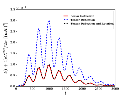
(a) Bin-1, $l^{\prime}=2-50$

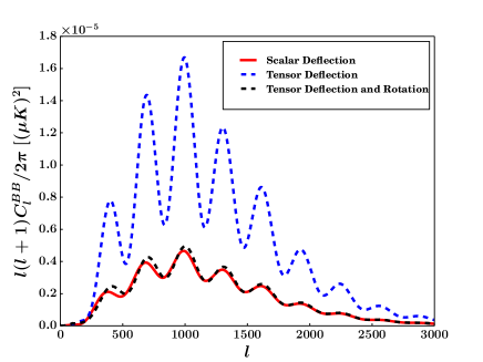
(b) Bin-2, $l^{\prime}=51-100$

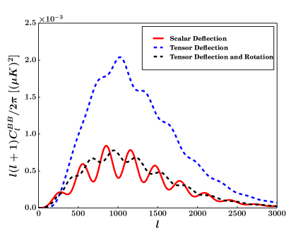
(c) Bin-3, $l^{\prime}=201-250$

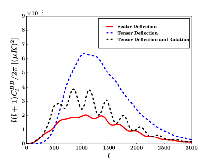
(d) Bin-4, $l^{\prime}=451-500$

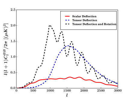
(e) Bin-5, $l^{\prime}=951-1000$

Figure 1: Comparison of individual contribution to lensed B-mode power spectrum due to scalar deflection, tensor deflection and tensor deflection + rotation for lensing power in five different bins. $l^{\prime}$ denotes the bin range of multipole over which $C_{l^{\prime}}^{\Omega\Omega}$ has nonzero power = $10^{-17}$

completely once the rotation is included. Depending on the nature of $C_{l}^{\Omega\Omega}$ there can be residual power at $C_{l}^{BB}$ at large $l$. This is due to the fact that the $C_{l}^{\psi\psi}$ which adds with the kernel given in Eq. (2.13), is dominant over $C_{l}^{\psi\Omega}$ at high $l$. Hence addition due to rotation term becomes important at high $l$. This is evident in Fig. 1(e) where contribution due to tensor deflection with rotation is dominant over contribution due to only tensor defection at some values of $l$. Also, it should be noted that the relative effect of rotation term is most evident when power in $C_{l}^{\Omega\Omega}$ is either at low $l$ or at high $l$.

Lensing potential $C_{l}^{\Omega\Omega}$ induced by SGWB provides a window to constrain $\Omega_{GW}$. Different models of generation of tensor perturbations predict different forms and amplitudes for $C_{l}^{\Omega\Omega}$ [5]. Each of this lensing potentials may not be detectable on their own. For example, [2] has shown that lensing potential introduced by inflationary gravitational wave background gives the lensing contribution which is below the cosmic variance. We do not address any particular model generating the lensing potential. Instead, we assume well motivated general forms of lensing potential and assess at what amplitude they produce any detectable effect on CMB through lensing. The method used in our analysis is presented in the following section.

3 Method

Curl deflection potential, $C_{l}^{\Omega\Omega}$ is related to the energy density of SGWB through the power spectrum of tensor perturbations, $P_{H}(k)$. Power spectrum of curl deflection potential $C_{l}^{\Omega\Omega}$ is [2]

$$C_{l}^{\Omega\Omega}=\frac{\pi}{l^{2}(l+1)^{2}}\frac{(l+2)!}{(l-2)!}\int d^{3}kP_{H}(k)|T_{l}^{H}(k)|^{2},$$ (3.1)

where $T_{l}^{H}(k)$ accounts for the evolution of tensor perturbations in the given universe and their projection onto the sphere. $T_{l}^{H}(k)$ is given by

$$T_{l}^{H}(k)=2k\int_{\eta_{s}}^{\eta_{0}}d\eta^{{}^{\prime}}T_{H}(k,\eta^{{}^{\prime}}-\eta_{s})\frac{j_{l}(k(\eta_{0}-\eta^{{}^{\prime}}))}{(k(\eta_{0}-\eta^{{}^{\prime}}))^{2}},$$ (3.2)

where $\eta$ is the conformal time. $\eta_{s}$ denotes the conformal time at source redshift and $\eta_{0}$ denotes conformal time at present epoch. $T_{H}(k,\eta)$ is the transfer function for tensor perturbations given by $3j_{1}(k\eta)/(k\eta)$. $T_{H}$ depends on $(\eta^{{}^{\prime}}-\eta_{s})$ and not only on $\eta^{{}^{\prime}}$. We adopt the following definition for the power spectrum $P_{H}(k)$ [2]

$$\langle H_{i}(\vec{k})H^{*}_{j}(\vec{k^{{}^{\prime}}})\rangle=(2\pi)^{3}P_{H}(k)\delta_{ij}\delta^{(3)}(\vec{k}-\vec{k^{{}^{\prime}}}),$$ (3.3)

where $H(\vec{k})$ is tensor metric perturbation. Tensor perturbations realized as SGWB contribute to the energy density of the universe. Spectral energy density of SGWB ($\rho_{GW}$) at present epoch is generally expressed in term of the density parameter $\Omega_{GW}$, which is

$$\Omega_{GW}(k)=\frac{1}{\rho_{c0}c^{2}}\frac{d\rho_{GW}(k,z=0)}{d\ln k},$$ (3.4)

where $\rho_{c0}=\frac{3H_{0}^{2}}{8\pi G}$ is the critical density of the universe at the present epoch. The spectral energy density, $\Omega_{GW}$ at the present epoch can be expressed as

$$\Omega_{GW}(k)=\frac{4\pi}{3}\Big{(}\frac{c}{H_{0}}\Big{)}^{2}k^{3}P_{H}(k)\Big{[}k\frac{dT_{H}(x)}{dx}\Big{]}^{2}_{k(\eta_{0}-\eta_{s})}.$$ (3.5)

It is known that a power law form of power spectrum $P_{H}(k)$ gives rise to the lensing potential $C_{l}^{\Omega\Omega}$ that can be approximated by a power law to good accuracy [22]. In particular $P_{H}(k)=k^{-n}$ gives $C_{l}^{\Omega\Omega}=Al^{-\alpha}$ where $\alpha=n+3$ and $A$ is the amplitude which depends on the source redshift. Motivated by this fact, we assume power law forms of $C_{l}^{\Omega\Omega}$ characterized by an amplitude $A$, power $\alpha$ and a cutoff in $l$, denoted by $l_{max}$. Given an $l_{max}$ and $\alpha$, we determine the value of $A$ which will produce a detectable effect on lensed $C_{l}^{BB}$. We denote the lensing contribution of $C_{l}^{\Omega\Omega}$ to $C_{l}^{BB}$ by $\delta\tilde{C}_{l}^{BB}$. To obtain this threshold we compare $\delta\tilde{C}_{l}^{BB}$ with the cosmic variance. For a given $\alpha$, we want to know the value of amplitude $A$ for which maxima of $\delta\tilde{C}_{l}^{BB}$ reaches a particular value. This particular value is chosen to be three times the value of the cosmic variance of lensed $C_{l}^{BB}$ due to $C_{l}^{\phi\phi}$ at the multipole where the maxima occur. This is an idealistic criteria which assumes zero noise experiment limited only by cosmic variance.

Once the constrained form of $C_{l}^{\Omega\Omega}$ is known, we use it to obtain the constrained form of $P_{H}(k)$. Eq. (3.1) shows that $C_{l}^{\Omega\Omega}$ is convolution of $P_{H}(k)$ and $|T_{l}^{H}(k)|^{2}$. A given a set of cosmological parameters completely determines $T_{l}^{H}(k)$. To obtain $P_{H}(k)$ for given $C_{l}^{\Omega\Omega}$ and $T_{l}^{H}(k)$ we use the Richardson-Lucy (RL) deconvolution algorithm [23, 24] This method has been used in the literature to deconvolve primordial power spectrum of scalar perturbations using WMAP and Planck data of CMB temperature anisotropies [25, 26, 27, 28]. To apply this method we write Eq. (3.1) in discrete form

$$C_{l}^{\Omega\Omega}=\sum_{i}G(l,k_{i})P_{H}(k_{i}),$$ (3.6)

where

$$G(l,k_{i})=\frac{4\pi^{2}}{l^{2}(l+1)}\frac{(l+2)!}{(l-2)!}\Delta k_{i}k_{i}^{2}|T^{H}_{l}(k_{i})|^{2}.$$ (3.7)

Given $C_{l}^{\Omega\Omega}$, $G(l,k_{i})$ and the initial guess for $P_{H}(k)$, RL method iteratively solves for the power spectrum using the following relation

$$P_{H}^{r+1}(k_{i})=P_{H}^{r}(k_{i})+P_{H}^{r}(k_{i})\sum_{l}G(l,k_{i})\frac{C^{\Omega\Omega}_{l}-C^{(r)}_{l}}{C^{(r)}_{l}}$$ (3.8)

at each $k_{i}$. Here $P_{H}^{r}(k_{i})$ is the power spectrum obtained after $r^{th}$ iteration. $C^{r}_{l}$ is the $C_{l}^{\Omega\Omega}$ recovered using Eq. (3.6) for $r^{th}$ iterate of the spectrum, $P^{r}_{H}(k)$

$$C_{l}^{r}=\sum_{i}G(l,k_{i})P^{r}_{H}(k_{i}).$$ (3.9)

We monitor the sum of square of relative error between recovered $C^{r}_{l}$ and input $C_{l}$ to decide when to stop the iterations. The iterations are carried out until the quantity

$$\sigma^{2}=\sum_{l}\Big{(}\frac{C^{\Omega\Omega}_{l}-C^{r}_{l}}{C_{l}^{\Omega\Omega}}\Big{)}^{2}$$ (3.10)

reaches a particular predetermined value. This controls the accuracy of recovered power spectrum. For our analysis we have taken the value of $\sigma^{2}$ such that the discrepancy of the recovered $P_{H}(k)$ will translate to negligible difference in the value of lensed $C_{l}^{BB}$. This discrepancy is set well below the cosmic variance of the lensed $C_{l}^{BB}$. We have tested our algorithm by implementing it on the $C_{l}^{\Omega\Omega}$ to recover $P_{H}(k)$ that is known beforehand. Our implementation of RL algorithm could recover $P_{H}(k)$ within above mentioned accuracy. The recovered $P_{H}(k)$ has wiggles peculiar to RL algorithm. We smooth out the wiggles in recovered $P_{H}(k)$. This $P_{H}(k)$ is then used to obtain the $\Omega_{GW}(k)$ using Eq. (3.5).

4 Results

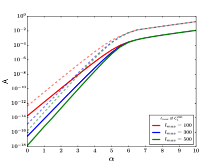
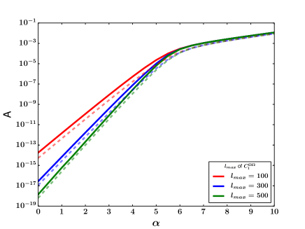
Figure 2: For the power-law form of $C_{l}^{\Omega\Omega}=Al^{-\alpha}$ as discussed in Sec. 3, we obtain the bounds on parameters $A$ for different values of $\alpha$ and $l_{max}$. (a) Continuous curves are for bounds using $C_{l}^{BB}$ while dashed curves are bounds using $C_{l}^{TT}$. Bounds obtained using $C_{l}^{BB}$ are stronger than those of $C_{l}^{TT}$. For $\alpha>6$, bounds on $A$ are insensitive to $l_{max}$. (b) Continuous curves are for bounds using $C_{l}^{BB}$ with rotation and dashed curves are for bounds using $C_{l}^{BB}$ without rotation.

In Fig. 2 we give bounds on $A$ for values of $\alpha$ ranging from $0$ to $10$. Results for different $l_{max}$ cutoff are given. Within the power law approximation considered here $\alpha=6$ corresponds to $P_{H}(k)=k^{-3}$, which is scale invariant power spectrum. Hence $\alpha>6$ corresponds to red $P_{H}(k)$ whereas $\alpha<6$ corresponds to blue $P_{H}(k)$. As a consequence bounds on $A$ are expected to be less sensitive to value of $l_{max}$ for $\alpha>6$. This is evident from the Fig. 2. For $\alpha>6$, all the curves corresponding to different $l_{max}$ give same bound on $A$. We carry out the same exercise with lensing of $C_{l}^{TT}$ and obtain the bounds on $A$, also shown in Fig. 2. The bounds on $A$ obtained using $C_{l}^{TT}$ are weaker roughly by one order of magnitude compared to the bounds from $C_{l}^{BB}$. In Fig. 2 we depict the bounds on $A$ with and without the rotation term obtained using $C_{l}^{BB}$. At higher values of $\alpha$ the value of $A$ becomes less sensitive to the rotation term. $C_{l}^{\Omega\Omega}$ with lower values of $\alpha$ have large power at low $l$ compared to those with higher values of $\alpha$. This leads to cancellation effect of rotation term being more effective for low $\alpha$ values compared to higher $\alpha$ values. Bounds obtained using $C_{l}^{TT}$ are not affected by rotation because rotation of polarization do not affect $C_{l}^{TT}$.

Given $\alpha$, and corresponding constrained $A$, we obtain allowed forms of $C_{l}^{\Omega\Omega}$. We use the RL algorithm to reconstruct the constrained $P_{H}(k)$. Given an $l_{max}$ and source redshift $z_{s}$, $P_{H}(k)$ can be constrained only up to $k_{max}=l_{max}/(\eta_{s}-\eta_{0})$. Hence, larger the source redshift smaller is the $k_{max}$ up to which we can constrain $P_{H}(k)$.

For any physical model, we expect a natural cut off in wavenumber ($k_{max}$) up to which $P_{H}(k)$ is non-zero. For $\alpha>6$ which corresponds to red spectra, $P_{H}(k)$ decreases with $k$ and for blue spectra with $\alpha<6$, $P_{H}(k)$ increases with $k$. Power spectrum of tensor perturbations from inflation as well as by second order effects in density perturbations both are red at the $k$ range we are interested in [5]. The power spectrum of [29] for tensor perturbations from second order effects generated at various redshifts is also red in nature. Blue spectrum is unlikely to be produced by such physical mechanisms at the $k$ range we are interested. So, we restrict our estimation of $\Omega_{GW}$ for red spectra, which correspond to $\alpha\geq 6$. This also ensures that we do not need to make any model dependent choice of $k_{max}$. We also note that the individual spectrum of tensor perturbations predicted in [5, 29] are not strong enough to contribute to detectable levels of lensed B-modes.

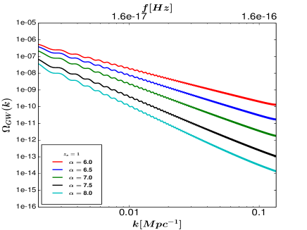
(a) Source redshift $z_{s}=1$

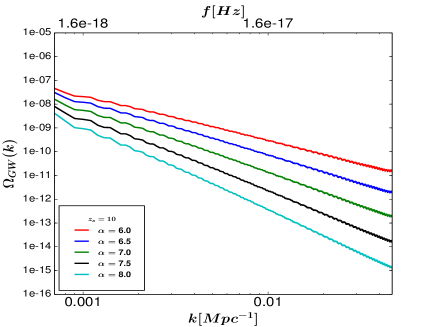
(b) Source redshift $z_{s}=10$

Figure 3: Constrained $\Omega_{GW}(k)$ for two source redshifts, $z_{s}=1$ and $z_{s}=10$. $\Omega_{GW}$ corresponding to red $P_{H}(k)$ obtained for different values of $\alpha$ and $l_{max}=500$ are shown. For given $l_{max}$ and $z_{s}$, $\Omega_{GW}$ is constrained up to $k_{max}=l_{max}/(\eta_{0}-\eta_{s})$. The results are given for the range of $k$ over which our recovery is faithful.

We use Eq. (3.5) to get $\Omega_{GW}(k)$ corresponding to reconstructed $P_{H}(k)$. Fig. 3 represent $\Omega_{GW}(k)$ for two source redshifts obtained using $C_{l}^{BB}$. We have taken the example of $l_{max}=500$ to elucidate our method. Curves shown in Fig. 3 are obtained using the running bin average of actual $\Omega_{GW}$ to reduce the wiggles which would otherwise be present due to the oscillatory behavior of the term $\frac{dT_{H}(x)}{dx}$ in Eq. (3.5). In Fig. 3 we see that for given $\alpha$, $\Omega_{GW}$ for redshift $z_{s}=10$ is smaller than that of redshift $z_{s}=1$. This is expected because to obtain a given amount of $C_{l}^{\Omega\Omega}$ one needs small power at high redshift than that at lower redshift.

5 Conclusion

Previous work argued that B-mode generated due to photon deflection are largely canceled by the rotation induced by tensor perturbations. Here we have demonstrated that this result is not generic and depend on the specifics of $C_{l}^{\Omega\Omega}$. The contribution of the rotation of polarization depends on the relative contribution of $C_{l}^{\psi\psi}$ and $C_{l}^{\psi\Omega}$ terms. Rotation term may contribute to lensing through subtraction or addition depending on the nature of curl deflection potential $C_{l}^{\Omega\Omega}$. Specifically, we note that the rotation term is most efficient at reducing power transfer from E-modes to B-modes when the power in $C_{l}^{\Omega\Omega}$ is concentrated at low $l$. Whereas, presence of more power at high $l$ in $C^{\Omega\Omega}_{l}$ decreases this efficiency (as depicted in Fig. 1).

The weak lensing of the CMB due to SGWB provides us a window to constrain SGWB of cosmological origin. In this work, we have exploited this effect to derive upper bounds on the energy density $\Omega_{GW}$ of the SGWB. To derive these constraints, we do not assume any particular model for the origin of SGWB, except that we present our constraints only for red spectra $P_{H}(k)$. We constrain the form of $\Omega_{GW}$ using idealistic constraints on $C_{l}^{\Omega\Omega}$. We first constrain the power law forms of $C_{l}^{\Omega\Omega}$ and translate it into upper bounds on $\Omega_{GW}$ sourced at a given redshift. In this paper, we present the model independent upper bound on $\Omega_{GW}$ spectrum which can lead to a particular observable imprint in CMB. Any model predicting $\Omega_{GW}(k)$ more than the ones depicted in Fig. 3 over the range of $k$ will be able to cast an observable signature on CMB $B$ mode polarization through lensing.

6 Acknowledgements

S.S. acknowledges University Grants Commission (UGC), India for providing the financial support as Senior Research Fellow. S.M. thanks Council of Scientific & Industrial Research (CSIR), India for financial support as Senior Research Fellow. The present work is carried out using the High Performance Computing facility at IUCAA.

References

- [1] S. Mollerach, Gravitational lensing on the cosmic microwave background by gravity waves, Phys.Rev. D57 (1998) 1303–1305, [astro-ph/9708196].
- [2] C. Li and A. Cooray, Weak Lensing of the Cosmic Microwave Background by Foreground Gravitational Waves, Phys.Rev. D74 (2006) 023521, [astro-ph/0604179].
- [3] T. Inagaki, K. Takahashi, and N. Sugiyama, Stochastic Gravitational Wave Background originating from Halo Mergers, Phys. Rev. D85 (2012) 104051, [arXiv:1204.1439].
- [4] C. Carbone, C. Baccigalupi, and S. Matarrese, The stochastic gravitational wave background from cold dark matter halos, Phys.Rev. D73 (2006) 063503, [astro-ph/0509680].
- [5] D. Sarkar, P. Serra, A. Cooray, K. Ichiki, and D. Baumann, Cosmic shear from scalar-induced gravitational waves, Phys. Rev. D77 (2008) 103515, [arXiv:0803.1490].
- [6] M. Maggiore, Gravitational wave experiments and early universe cosmology, Physics Reports 331 (2000), no. 6 283 – 367.
- [7] Virgo, LIGO Scientific Collaboration, B. P. Abbott et al., Observation of Gravitational Waves from a Binary Black Hole Merger, Phys. Rev. Lett. 116 (2016), no. 6 061102, [arXiv:1602.0383].
- [8] Virgo, LIGO Scientific Collaboration, B. P. Abbott et al., GW150914: Implications for the stochastic gravitational wave background from binary black holes, Phys. Rev. Lett. 116 (2016), no. 13 131102, [arXiv:1602.0384].
- [9] A. Rotti and T. Souradeep, A New Window into Stochastic Gravitational Wave Background, Phys. Rev. Lett. 109 (2012) 221301, [arXiv:1112.1689].
- [10] A. Cooray, M. Kamionkowski, and R. R. Caldwell, Cosmic shear of the microwave background: The Curl diagnostic, Phys. Rev. D71 (2005) 123527, [astro-ph/0503002].
- [11] S. Dodelson, E. Rozo, and A. Stebbins, Primordial gravity waves and weak lensing, Phys. Rev. Lett. 91 (2003) 021301, [astro-ph/0301177].
- [12] H. Padmanabhan, A. Rotti, and T. Souradeep, A comparison of CMB lensing efficiency of gravitational waves and large scale structure, Phys.Rev. D88 (2013) 063507, [arXiv:1307.2355].
- [13] L. Dai, Rotation of the cosmic microwave background polarization from weak gravitational lensing, Phys. Rev. Lett. 112 (2014), no. 4 041303, [arXiv:1311.3662].
- [14] T. Namikawa, D. Yamauchi, and A. Taruya, Future detectability of gravitational-wave induced lensing from high-sensitivity CMB experiments, Phys. Rev. D91 (2015), no. 4 043531, [arXiv:1411.7427].
- [15] Planck Collaboration, P. A. R. Ade et al., Planck 2013 results. XVI. Cosmological parameters, Astron. Astrophys. 571 (2014) A16, [arXiv:1303.5076].
- [16] T. Okamoto and W. Hu, CMB lensing reconstruction on the full sky, Phys. Rev. D67 (2003) 083002, [astro-ph/0301031].
- [17] T. Namikawa, D. Yamauchi, and A. Taruya, Full-sky lensing reconstruction of gradient and curl modes from CMB maps, JCAP 1201 (2012) 007, [arXiv:1110.1718].
- [18] A. Stebbins, Weak lensing on the celestial sphere, astro-ph/9609149.
- [19] D. Yamauchi, T. Namikawa, and A. Taruya, Full-sky formulae for weak lensing power spectra from total angular momentum method, JCAP 1308 (2013) 051, [arXiv:1305.3348].
- [20] A. Challinor and A. Lewis, Lensed CMB power spectra from all-sky correlation functions, Phys. Rev. D71 (2005) 103010, [astro-ph/0502425].
- [21] W. Hu, Weak lensing of the CMB: A harmonic approach, Phys. Rev. D62 (2000) 043007, [astro-ph/0001303].
- [22] L. Book, M. Kamionkowski, and F. Schmidt, Lensing of 21-cm Fluctuations by Primordial Gravitational Waves, Phys. Rev. Lett. 108 (2012) 211301, [arXiv:1112.0567].
- [23] W. H. Richardson, Bayesian-based iterative method of image restoration, J. Opt. Soc. Am. 62 (Jan, 1972) 55–59.
- [24] L. B. Lucy, An iterative technique for the rectification of observed distributions, Astron. J. 79 (1974) 745–754.
- [25] A. Shafieloo and T. Souradeep, Primordial power spectrum from WMAP, Phys. Rev. D70 (2004) 043523, [astro-ph/0312174].
- [26] D. K. Hazra, A. Shafieloo, and T. Souradeep, Primordial power spectrum: a complete analysis with the WMAP nine-year data, JCAP 1307 (2013) 031, [arXiv:1303.4143].
- [27] D. K. Hazra, A. Shafieloo, and T. Souradeep, Primordial power spectrum from Planck, JCAP 1411 (2014), no. 11 011, [arXiv:1406.4827].
- [28] G. Nicholson and C. R. Contaldi, Reconstruction of the Primordial Power Spectrum using Temperature and Polarisation Data from Multiple Experiments, JCAP 0907 (2009) 011, [arXiv:0903.1106].
- [29] J. Adamek, R. Durrer, and M. Kunz, N-body methods for relativistic cosmology, Class. Quant. Grav. 31 (2014), no. 23 234006, [arXiv:1408.3352].