Hiding Planets Behind a Big Friend: Mutual Inclinations of Multi-Planet Systems with External Companions

Abstract

The Kepler mission has detected thousands of planetary systems with 1-7 transiting planets packed within 0.7 au from their host stars. There is an apparent excess of single-transit planet systems that cannot be explained by transit geometries alone, when a single planetary mutual inclination dispersion is assumed. This suggests that the observed compact planetary systems have at least two different architectures. We present a scenario where the “Kepler dichotomy” may be explained by the action of an external giant planet or stellar companion misaligned with the inner multi-planet system. The external companion excites mutual inclinations of the inner planets, causing such systems to appear as “Kepler singles” in transit surveys. We derive approximate analytic expressions (in various limiting regimes), calibrated with numerical calculations, for the mutual inclination excitations for various planetary systems and perturber properties (mass $m_{p}$, semi-major axis $a_{p}$ and inclination $\theta_{p}$). In general, the excited mutual inclination increases with $m_{p}/a_{p}^{3}$ and $\theta_{p}$, although secular resonances may lead to large mutual inclinations even for small $\theta_{p}$. We discuss the implications of our results for understanding the dynamical history of transiting planet systems with known external perturbers.

1 Introduction

NASA’s Kepler mission has discovered $\sim 4700$ planet candidates (as of May 2016), about half of which are confirmed planets (e.g. Mullally et al. 2015; Coughlin et al. 2016; Morton et al. 2016). Most of these planets are super-Earths or sub-Neptunes (with radii 1.2-3$R_{\oplus}$), and have orbital periods less than 200 days. Among the $n_{\rm tran}=3606$ Kepler planetary systems, $80\%$ have one transiting planet, and $20\%$ have 2-7 transiting planets [The number of systems with $N_{\rm tran}$ planets is $n(N_{\rm tran})=2871,\,492,\,158,\,61,\,20,\,3,\,1$ for $N_{\rm tran}=1,2,\cdots,7$]. The observed transit multiplicity distribution, $f(N_{\rm tran})=n(N_{\rm tran})/n_{\rm tran}$, and its dependence on the sizes and periods of planets, contain useful information on the architecture of compact planetary systems, such as the true planet multiplicity, the mutual inclinations, and orbital spacings between adjacent planets. In general, there exists a degeneracy between these (underlying) quantities in producing the same $f(N_{\rm tran})$. For example, larger planet spacings and mutual inclinations will raise the relative number of single-transit systems (Lissauer et al. 2011; Tremaine & Dong 2012). This degeneracy can be partially lifted by combining the statistics of $f(N_{\rm tran})$ with the result of RV surveys (Tremaine & Dong 2012; Figueira et al. 2012), or using the transit duration ratios of different planets orbiting the same star (Fabrycky et al. 2014). The general conclusion from a number of studies is that Kepler compact planetary systems are flat, with the inclination dispersion of order a few degrees (Lissauer et al. 2011; Tremaine & Dong 2012; Figueira et al. 2012; Johansen et al. 2012; Fang & Margot 2012; Fabrycky et al. 2014).

It has been noted that models with a single mutual inclination dispersion (e.g. in a Rayleigh distribution) fall short in explaining the large number of single-transit ($N_{\rm tran}=1$) systems relative to multiple-transit (higher-$N_{\rm tran}$) systems by a factor of two or more (Lissauer et al. 2011; Johansen et al. 2012; Weissbein et al. 2012; Ballard & Johnson 2016). This suggests that the Kepler planetary systems may consist of at least two underlying populations with different architectures: The first has many ($\mathrel{\raise 1.29167pt\hbox{$>$}\mkern-14.0mu\lower 2.58334pt\hbox{$\sim$}}6$) planets with small ($\mathrel{\raise 1.29167pt\hbox{$<$}\mkern-14.0mu\lower 2.58334pt\hbox{$\sim$}}2^{\circ}$) mutual inclinations, and accounts for the majority of the $N_{\rm tran}\geq 2$ systems; the second has fewer planets or higher mutual inclinations, and accounts for a significant portion of the observed single-transit systems. This is the so-called “Kepler Dichotomy”. Xie et al. (2014) found that the multi-transit systems are more likely to exhibit detectable transit timing variations than the single-transit systems, suggesting that the former are more closely packed than the latter. Morton & Winn (2014) found that the obliquities of stars with a single transiting planet are systematically larger than those with multiple transiting planets (see Albrecht et al. 2013), again suggesting that a substantial fraction of Kepler’s single-transit systems are dynamically hotter than the flat multiple-transit systems.

The origin of the Kepler dichotomy is unknown. The observed Kepler multi-planet systems appear to be tightly packed and close to the edge of instability (Fang & Margot 2013; Pu & Wu 2015; Volk & Gladman 2015). Thus a dichotomy in planetary architectures may arise from the long-term evolution of dynamically full systems. In this picture, the more densely packed systems underwent dynamical instability, leading to planet collision/consolidation and the formation of Kepler “singles” (Pu & Wu 2015; Volk & Gladman 2015). It is unclear to what extent dynamical instability can account for the Kepler dichotomy quantitatively, as the observed Kepler multi’s are sufficiently “cold” and not massive enough to experience appreciable inclination excitation or dynamical instability within the stellar lifetime (Johansen et al. 2012; Becker & Adams 2016). On the other hand, the Kepler dichotomy may have a primordial origin, and results from the in-situ assembly of planetesimal disks (Hansen & Murray 2013) with different masses and density profiles (Moriarty & Ballard 2015).

In this paper we study the excitation of mutual inclinations in a compact multi-planet system by an external giant planet or stellar companion (Sections 2 and 3). In general, the giant planet may be on a misaligned orbit relative to the inner planetary system, as a result of warp in protoplanetary disks (e.g., Foucart & Lai 2011,2014) or strong scatterings between multiple giants (Juric & Tremaine 2008; Chatterjee et al. 2008). A distant stellar companion may also be inclined because of its misaligned orbital angular momentum at birth (e.g. Hale 1994). By exciting mutual inclinations of the inner planets, the giant planet can “heat up” the inner multi-planet system, causing it to appear as a single-transit system.

Since $\sim 50\%$ of the solar-type stars are in binaries, it is not surprising that many exoplanetary systems (including Kepler planet candidates) have been found to have external binary companions with a range of separations (e.g., Baranec et al. 2016). There is observational evidence that relatively close-by stellar companions (with separation $\mathrel{\raise 1.29167pt\hbox{$<$}\mkern-14.0mu\lower 2.58334pt\hbox{$\sim$}}20-50$ au) tend to reduce the planet formation efficiency (e.g., Wang et al. 2015a; Kraus et al. 2016; Ngo et al. 2016). Wang et al. (2015b) found that $5\pm 5\%$ of Kepler multi’s have stellar companions at separation 1-100 au, compared to $21\%$ for field stars in the solar neighborhood, suggesting that such companions can misalign or disrupt multi-planet systems. On the other hand, RV surveys continue to reveal a population of giant planets at large distances ($\mathrel{\raise 1.29167pt\hbox{$>$}\mkern-14.0mu\lower 2.58334pt\hbox{$\sim$}}$ a few au) from their host stars (e.g., Marmier et al. 2013; Feng et al. 2015; Moutou et al. 2015; Rowan et al. 2016; Wittenmyer et al. 2016; Bryan et al. 2016). The Keck survey suggests that about $20\%$ of solar-type stars could host gas giants within 20 au (Cumming et al. 2008), while HARPS finds that $14\%$ of such stars host giant planets with periods less than 10 years. Because of the limited time span and the faint magnitudes of Kepler stars, the current census of distant giant companions to Kepler compact systems is rather incomplete. Nevertheless, a number of such long-period companions or candidates have been found using the transit method (Schmitt et al. 2014; Uehara et al. 2016) and the RV method (e.g., Kepler-48, Kepler-56, Kepler-68, Kepler-90, Kepler-454); a number of non-Kepler “inner compact planets + giant companion” systems have also been found (e.g., GJ 832, WASP-47) – see Section 4 for applications of our theory to some of these systems. Bryan et al. (2016) reported that about $50\%$ of one and two-planet systems discovered by RV have companions in the 1-20$M_{J}$ and 5-20 au range. All these results indicate that external ($\mathrel{\raise 1.29167pt\hbox{$>$}\mkern-14.0mu\lower 2.58334pt\hbox{$\sim$}}1$ au) giant planet companions are common around hot/warm ($\mathrel{\raise 1.29167pt\hbox{$<$}\mkern-14.0mu\lower 2.58334pt\hbox{$\sim$}}1$ au) planets, and may significantly shape the architecture of the inner planetary systems.

We note that the possible role of external companions on compact planetary systems has often been noted (e.g. Lissauer et al. 2011) and formal secular theories (with various approximations) suitable for such study have been presented before (e.g. Tremaine et al. 2009; Boue & Fabrycky 2014). Our paper makes progress on this problem by deriving simple approximate analytic expressions (in various limiting regimes), calibrated with numerical results (Sections 2 and 3), that allow us to answer the question: Given an inner planetary system, what are the mutual inclinations excited by an external perturber of mass $m_{p}$, semi-major axis $a_{p}$ and inclination $\theta_{p}$? In general, a “strong” perturber (with large $m_{p}/a_{p}^{3}$) with high $\theta_{p}$ leads to larger mutual inclinations in the inner planets. But our work also reveals that under some conditions, large mutual inclinations can be generated even for small $\theta_{p}$ ($\mathrel{\raise 1.29167pt\hbox{$<$}\mkern-14.0mu\lower 2.58334pt\hbox{$\sim$}}1^{\circ}$) because of secular resonances.

2 Two-Planet Systems with External Perturber

Consider two planets (mass $m_{1}$ and $m_{1}$) in circular orbits (semi-major axes $a_{1}$ and $a_{2}$, with $a_{2}>a_{1}$) around a central star (mass $M_{\star}$). The two planets are initially coplanar. An external perturber (mass $m_{p}$) moves in a circular inclined orbit , with semi-major axis $a_{p}$ ($>a_{1},a_{2}$) and inclination angle $\theta_{p}$. How does the mutual inclination of the two inner planets evolve?

We denote the angular momentum vectors to the three planets by $\bm{L}_{1}=L_{1}\bm{\hat{l}}_{1}$, $\bm{L}_{2}=L_{2}\bm{\hat{l}}_{2}$ and $\bm{L}_{p}=L_{p}\bm{\hat{l}}_{p}$, where $\bm{\hat{l}}_{1}$, $\bm{\hat{l}}_{2}$ and $\bm{\hat{l}}_{p}$ are unit vectors. When $L_{p}\gg L_{1},~{}L_{2}$, the unit vector $\bm{\hat{l}}_{p}$ is fixed in time. The evolution of $\bm{\hat{l}}_{1}$, $\bm{\hat{l}}_{2}$ is governed by

$${\text{d}\bm{\hat{l}}_{1}\over\text{d}t}=\omega_{12}(\bm{\hat{l}}_{1}\cdot\bm{\hat{l}}_{2})(\bm{\hat{l}}_{1}\times\bm{\hat{l}}_{2})+\Omega_{1p}(\bm{\hat{l}}_{1}\cdot\bm{\hat{l}}_{p})(\bm{\hat{l}}_{1}\times\bm{\hat{l}}_{p}),$$ (1)

$${\text{d}\bm{\hat{l}}_{2}\over\text{d}t}=\omega_{21}(\bm{\hat{l}}_{1}\cdot\bm{\hat{l}}_{2})(\bm{\hat{l}}_{2}\times\bm{\hat{l}}_{1})+\Omega_{2p}(\bm{\hat{l}}_{2}\cdot\bm{\hat{l}}_{p})(\bm{\hat{l}}_{2}\times\bm{\hat{l}}_{p}).$$ (2)

Here $\omega_{12}$ measures the precession rate of $\bm{\hat{l}}_{1}$ around $\bm{\hat{l}}_{2}$ (driven by $m_{2}$), and $\Omega_{1p}$ the precession rate of $\bm{\hat{l}}_{1}$ around $\bm{\hat{l}}_{p}$ (driven by $m_{p}$):

$$\omega_{12}={Gm_{1}m_{2}a_{1}\over 4a_{2}^{2}L_{1}}b_{3/2}^{(1)}\!\left({a_{1}\over a_{2}}\right),$$ (3)

$$\Omega_{1p}={Gm_{1}m_{p}a_{1}\over 4a_{p}^{2}L_{1}}b_{3/2}^{(1)}\!\left({a_{1}\over a_{p}}\right),$$ (4)

where $b_{3/2}^{(1)}(\chi)$ is the Laplace coefficient:

$$b_{3/2}^{(1)}(\chi)=\frac{2}{\pi}\int_{0}^{\pi}\frac{\cos\phi\,\text{d}\phi}{(1-2\chi\cos\phi+\chi^{2})^{3/2}}.$$ (5)

Similar expressions apply to $\omega_{21}$ and $\Omega_{2p}$. Clearly

$${\omega_{21}\over\omega_{12}}={L_{1}\over L_{2}}={m_{1}\over m_{2}}\left({a_{1}\over a_{2}}\right)^{1/2},$$ (6)

$${\Omega_{2p}\over\Omega_{1p}}=\left(\!{a_{2}\over a_{1}}\!\right)^{\!1/2}{b_{3/2}^{(1)}(a_{2}/a_{p})\over b_{3/2}^{(1)}(a_{1}/a_{p})}.$$ (7)

Note that Eqs. (1)-(4) are approximate but become exact in two limiting cases: (i) $\bm{\hat{l}}_{1}$, $\bm{\hat{l}}_{2}$ and $\bm{\hat{l}}_{p}$ are nearly aligned (e.g., Tremaine 1991); (ii) $\chi\ll 1$, in which case the quadrupole approximation is accurate and $b_{3/2}^{(1)}(\chi)=3\chi[1+(15/8)\chi^{2}+(175/64)\chi^{4}+\cdots]\simeq 3\chi$ (Murray & Dermott 1999).

2.1 Numerical Result

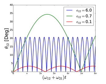
Figure 1: Time evolution of the mutual inclination angle between two inner planets in the presence of an external inclined perturber (at $\theta_{p}=10^{\circ}$). The two planets have mass ratio $m_{2}/m_{1}=10$, with $a_{1}=0.3$ au, $a_{2}=0.5$ au and are initially aligned. Different curves are for different values of $\epsilon_{12}$, corresponding to different strengths of the perturber ($m_{p}/a_{p}^{3}$). For $\epsilon_{12}\ll 1$, $\theta_{12}$ oscillates with the characteristic frequency $(\omega_{12}+\omega_{21})$ (see Eq. 19); for $\epsilon_{12}\gg 1$, the characteristic frequency is $(\Omega_{2p}-\Omega_{1p})\cos\theta_{p}$ (see Eq. 22); near the resonance ($\epsilon_{12}\sim 1$; see the green curve), the characteristic frequency is much smaller.

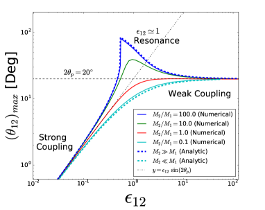
Figure 2: Maximum mutual inclination between two inner planets ($m_{1},m_{2}$) in the presence of an external perturber ($m_{p}$). The inner planets are initially coplanar ($\theta_{12}=0$) and inclined relative to the perturber at $\theta_{p}=10^{\circ}$. The two planets are located at $a_{1}=0.3$ au and $a_{2}=0.5$ au (but only $a_{2}/a_{1}$ affects the result). The different curves correspond to different mass ratios, as indicated. The dimensionless parameter $\epsilon_{12}$ (see Eq. 8 or 12) is varied by varying the “strength”of the perturber, $m_{p}/a_{p}^{3}$. Analytical results in the strong coupling and weak coupling limits are also shown. A resonance feature is present when $m_{2}/m_{1}\mathrel{\raise 1.29167pt\hbox{$>$}\mkern-14.0mu\lower 2.58334pt\hbox{$\sim$}}1$.

We integrate Eqs. (1)-(2) with an initially aligned pair of inner planets, and an inclined external perturber at $\theta_{p}=10^{\circ}$. Figure 1 shows a few examples of the time evolution of the mutual inclination angle ($\theta_{12}$) between the two inner planets, for $a_{1}=0.3$ au, $a_{2}=0.5$ au, $m_{2}/m_{1}=10$, and several values of $\epsilon_{12}$, as defined by

$$\epsilon_{12}\equiv{\Omega_{2p}-\Omega_{1p}\over\omega_{12}+\omega_{21}}.$$ (8)

Figure 2 depicts the maximum mutual inclination, $(\theta_{12})_{\rm max}$, as a function of $\epsilon_{12}$ for several different values of mass ratio $m_{2}/m_{1}$. The dimensionless parameter $\epsilon_{12}$ measures whether the inner planets are strongly coupled ($\epsilon_{12}\ll 1$) or weakly coupled ($\epsilon_{12}\gg 1$); see below. Note that $\epsilon_{12}$ can be written as

$$\epsilon_{12}={\hat{\Omega}}_{1p}\,\,{(\Omega_{2p}/\Omega_{1p})-1\over 1+(L_{1}/L_{2})}.$$ (9)

Here $L_{1}/L_{2}=(m_{1}/m_{2})(a_{1}/a_{2})^{1/2}$ is the ratio of the planet’s angular momenta , $\Omega_{2p}/\Omega_{1p}$ is given by Eq. (7), which simplifies to

$${\Omega_{2p}\over\Omega_{1p}}\approx\left({a_{2}\over a_{1}}\right)^{3/2}$$ (10)

in the quadrupole approximation (valid for $a_{p}\gg a_{2},a_{1}$), and

$${\hat{\Omega}}_{1p} \equiv {\Omega_{1p}\over\omega_{12}}={m_{p}\over m_{2}}\,{a_{2}^{2}\,b_{3/2}^{(1)}(a_{1}/a_{p})\over a_{p}^{2}\,b_{3/2}^{(1)}(a_{1}/a_{2})}$$ (11)

$$\approx {m_{p}\over m_{2}}\left({a_{2}\over a_{p}}\right)^{3}\,{3a_{1}/a_{2}\over b_{3/2}^{(1)}(a_{1}/a_{2})},$$

where the last equality assumes $a_{p}\gg a_{1}$. Thus

$$\epsilon_{12}\approx\left({m_{p}\over 10^{3}m_{2}}\right)\left({10a_{2}\over a_{p}}\right)^{3}\left[{3a_{1}/a_{2}\over b_{3/2}^{(1)}(a_{1}/a_{2})}\right]\,{(a_{2}/a_{1})^{3/2}-1\over 1+(L_{1}/L_{2})}.$$ (12)

For given inner planet parameters ($m_{1,2}$ and $a_{1,2}$ – in fact, only the ratios $m_{2}/m_{1}$ and $a_{2}/a_{1}$ matter), the result for $(\theta_{12})_{\rm max}$ depends on $\theta_{p}$ and on $m_{p}$ and $a_{p}$ through the combination $m_{p}/a_{p}^{3}$ (for $a_{p}\gg a_{1},a_{2}$).

In the following subsections we discuss the the behaviors of $(\theta_{12})_{\rm max}$ in the limits of $\epsilon_{12}\ll 1$ (strong coupling) and $\epsilon_{12}\gg 1$ (weak coupling), and as well as the resonance feature around $\epsilon_{12}\sim 1$.

2.2 Strong Coupling Limit: $\epsilon_{12}\ll 1$

In the strong coupling limit, with $\epsilon_{12}\ll 1$ (see Eq. 8), we expect $\bm{\hat{l}}_{1}$ and $\bm{\hat{l}}_{2}$ to stay close to alignment. Let $\bm{L}=\bm{L}_{1}+\bm{L}_{2}\equiv L\bm{\hat{l}}$ be the total angular momentum of the two inner planets, with $L\simeq L_{1}+L_{2}$. From Eqs. (1)-(2), we find

$${\text{d}\bm{\hat{l}}\over\text{d}t}\simeq\Omega_{L}(\bm{\hat{l}}\cdot\bm{\hat{l}}_{p})(\bm{\hat{l}}\times\bm{\hat{l}}_{p}),$$ (13)

where $-\Omega_{L}(\bm{\hat{l}}\cdot\bm{\hat{l}}_{p})$ is the precession rate of $\bm{\hat{l}}$ around $\bm{\hat{l}}_{p}$, with

$$\Omega_{L}\simeq{L_{1}\Omega_{1p}+L_{2}\Omega_{2p}\over L_{1}+L_{2}}.$$ (14)

In the frame corotating with $\bm{\hat{l}}$, we have

$$\biggl{(}{\text{d}\bm{\hat{l}}_{1}\over\text{d}t}\biggr{)}_{\rm rot}={\text{d}\bm{\hat{l}}_{1}\over\text{d}t}+\Omega_{L}(\bm{\hat{l}}\cdot\bm{\hat{l}}_{p})(\bm{\hat{l}}_{p}\times\bm{\hat{l}}_{1})$$

$$\simeq\left[\Bigl{(}\Omega_{L}\bm{\hat{l}}\!\cdot\bm{\hat{l}}_{p}-\Omega_{1p}\bm{\hat{l}}_{1}\!\cdot\bm{\hat{l}}_{p}\Bigr{)}\bm{\hat{l}}_{p}-\omega_{12}(\bm{\hat{l}}_{1}\!\cdot\bm{\hat{l}}_{2})\bm{\hat{l}}_{2}\right]\times\bm{\hat{l}}_{1}.$$ (15)

Let $\bm{\hat{l}}_{1,2}=\bm{\hat{l}}+\Delta{\bm{l}}_{1,2}$, with $|\Delta{\bm{l}}_{1,2}|\sim\epsilon_{12}\ll 1$. Note that

$$L_{1}\Delta{\bm{l}}_{1}+L_{2}\Delta{\bm{l}}_{2}\simeq 0.$$ (16)

Equation (15) then becomes, to leading order in $\epsilon_{12}$,

$$\biggl{(}{\text{d}\Delta{\bm{l}}_{1}\over\text{d}t}\biggr{)}_{\rm rot}\simeq-(\omega_{12}+\omega_{21})\bm{\hat{l}}\times\Delta{\bm{l}}_{1}+(\Omega_{1p}-\Omega_{L})(\bm{\hat{l}}\cdot\bm{\hat{l}}_{p})(\bm{\hat{l}}\times\bm{\hat{l}}_{p}),$$ (17)

For $\Delta{\bm{l}}_{1}(t=0)=0$, the leading-order solution is

$$\Delta{\bm{l}}_{1}(t)\simeq{L_{2}\over L}\epsilon_{12}\cos\theta_{p}\Bigl{[}(1-\cos\tau_{12})(\bm{\hat{l}}_{p}\!\times\!\bm{\hat{l}})\!\times\!\bm{\hat{l}}$$

$$\qquad\quad~{}~{}~{}+\sin\tau_{12}\,(\bm{\hat{l}}_{p}\!\times\!\bm{\hat{l}})\Bigr{]},$$ (18)

where we have used $\bm{\hat{l}}\cdot\bm{\hat{l}}_{p}=\cos\theta_{p}$ and $\tau_{12}\equiv(\omega_{12}+\omega_{21})t$. Using Eqs. (18) and (16), we then find that the mutual inclination angle $\theta_{12}$ between $\bm{\hat{l}}_{1}$ and $\bm{\hat{l}}_{2}$ is given by

$$\left|\sin\theta_{12}\right|=\left|\bm{\hat{l}}_{1}\times\bm{\hat{l}}_{2}\right|\simeq\epsilon_{12}\left|\sin 2\theta_{p}\sin{\tau_{12}\over 2}\right|.$$ (19)

Thus, the maximum and the RMS values of $\left|\sin\theta_{12}\right|$ are

$$\left|\sin\theta_{12}\right|_{\rm max}\simeq\epsilon_{12}\left|\sin 2\theta_{p}\right|,$$ (20)

$$\left\langle\sin^{2}\!\theta_{12}\right\rangle^{\!1/2}\simeq{1\over\sqrt{2}}\epsilon_{12}\left|\sin 2\theta_{p}\right|.$$ (21)

2.3 Weak Coupling Limit: $\epsilon_{12}\gg 1$

In the weak coupling limit, with $\epsilon_{12}\gg 1$, the vectors $\bm{\hat{l}}_{1}$ and $\bm{\hat{l}}_{2}$ precess around $\bm{\hat{l}}_{p}$ independently, with constant $\bm{\hat{l}}_{1}\cdot\bm{\hat{l}}_{p}\simeq\bm{\hat{l}}_{2}\cdot\bm{\hat{l}}_{p}\simeq\cos\theta_{p}$. Thus

$$\left|\bm{\hat{l}}_{1}\times\bm{\hat{l}}_{2}\right|^{2}\simeq\sin^{2}\!2\theta_{p}\,\sin^{2}\!\Bigl{(}{\Delta\phi_{12}\over 2}\Bigr{)}+\sin^{4}\!\theta_{p}\,\sin^{2}\!(\Delta\phi_{12}),$$ (22)

where $\Delta\phi_{12}\simeq(\Omega_{2p}-\Omega_{1p})(\cos\theta_{p})t$. The maximum of $\theta_{12}$ and the RMS value of $\left|\sin\theta_{12}\right|$ are

$$(\theta_{12})_{\rm max}\simeq 2\theta_{p},$$ (23)

$$\left\langle\sin^{2}\!\theta_{12}\right\rangle^{\!1/2}\simeq{1\over\sqrt{2}}\left(\sin^{2}\!2\theta_{p}+\sin^{4}\!\theta_{p}\right)^{1/2}.$$ (24)

2.4 Resonance

Figure 2 reveals that when $m_{2}\mathrel{\raise 1.29167pt\hbox{$>$}\mkern-14.0mu\lower 2.58334pt\hbox{$\sim$}}m_{1}$ (i.e., the outer planet is more massive than the inner planet), a resonance feature appears around $\epsilon_{12}\sim 1$. At the resonance, $(\theta_{12})_{\rm max}$ can become much larger than the weak-coupling limit, $2\theta_{p}$. When $m_{1}\mathrel{\raise 1.29167pt\hbox{$>$}\mkern-14.0mu\lower 2.58334pt\hbox{$\sim$}}m_{2}$, no resonance feature exists.

This resonance feature can be understood analytically in the limit when the planetary system contains a “dominant” planet (labeled “d”) which is much more massive than the other planet (labeled “j”), i.e., $m_{d}\gg m_{j}$. In Appendix A we develop the Hamiltonian theory for such systems. We show that for $\theta_{p}\ll 1$, a sharp resonance appears at $|\epsilon_{jd}|=1$, or

$$\Omega_{dp}=\Omega_{jp}+\omega_{jd},~{}~{}\Bigl{(}{\rm resonance~{}for}~{}{m_{d}\over m_{j}}\gg 1,\,\theta_{p}\ll 1\Bigr{)}.$$ (25)

This resonance condition is easy to interpret physically: The dominant planet experiences nodal precession at the frequency $\Omega_{dp}$ driven by the perturber, while the sub-dominant planet $m_{j}$ precesses at the rate $(\Omega_{jp}+\omega_{jd})$ driven by both the perturber and the dominant planet; resonance occurs when these two precession frequencies match. Clearly, to satisfy Eq. (25) requires $\Omega_{dp}>\Omega_{jp}$, or $a_{d}>a_{j}$, i.e., the dominant planet exterior to the sub-dominant planet. Near the resonance, the maximum mutual inclination behaves as (see Appendix A)

$$(\theta_{jd})_{\rm max}\simeq{2\epsilon_{jd}\theta_{p}\over|\epsilon_{jd}-1|}$$ (26)

(valid for general $\epsilon_{jd}$ but $\theta_{p},\theta_{jd,{\rm max}}\ll 1$). This provides an estimate for the “width” of the resonance for $\theta_{p}\ll 1$).. As $\theta_{p}$ increases, the resonance becomes broader and is shifted slightly to smaller $\epsilon_{12}$ (see Fig. 3). Also, as the mass ratio $m_{d}/m_{j}$ decreases, the resonance feature gradually become “smoothed” out and disappears when $m_{d}/m_{j}\mathrel{\raise 1.29167pt\hbox{$<$}\mkern-14.0mu\lower 2.58334pt\hbox{$\sim$}}1$ (see Fig. 2).

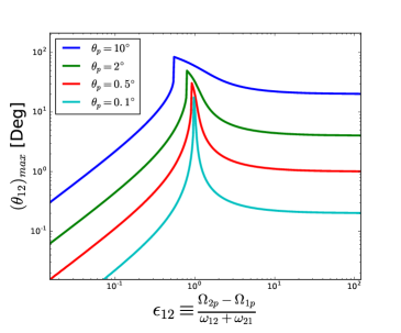
Figure 3: Maximum misalignment angle between two inner planets in the presence of an external perturber, as a function of $\epsilon_{12}$, in the limit of $m_{2}\gg m_{1}$. Note that in this limit, $\omega_{21}=(L_{1}/L_{2})\omega_{12}\ll\omega_{12}$. The two planets are located at $a_{1}=0.3$ au and $a_{2}=0.5$ au. Different curves correspond to different inclination angles ($\theta_{p}$) of the external perturber. These curves are obtained analytically by solving Eq. (A8) derived in Appendix A. The resonant feature is most prominent for $\theta_{p}\ll 1$ and is located at $\epsilon_{12}=1$ in the $\theta_{p}\rightarrow 0$ limit. As $\theta_{p}$ increases, the resonance feature is broadened and shifted to slightly smaller $\epsilon_{12}$.

3 Multi-Planet Systems with External Perturber

The evolution equations for the orientations of multi-planet ($N>2$) systems with an external perturber can be easily can be generalized (see Appendix B). Figures 4-6 show some numerical results for a 4-planet system ($N=4$) in the presence of an external perturber. To characterize the mutual misalignment of the planets for a wide range of parameters, we take the dominant planet (the one with the largest mass, labeled “d”) in the system and measure the relative inclination ($\bm{\hat{l}}_{j}$) of the other planets with respect to $\bm{\hat{l}}_{d}$. We define the RMS of $|\bm{\hat{l}}_{j}\times\bm{\hat{l}}_{d}|$ as

$${\rm RMS}\left(\sin\!\Delta\theta\right)\equiv\left({1\over N-1}\Bigl{\langle}\sum_{j\neq d}\bigl{|}\bm{\hat{l}}_{j}\times\bm{\hat{l}}_{d}\bigr{|}^{2}\Bigr{\rangle}\right)^{\!1/2},$$ (27)

and the mutual inclination spread as

$$\sigma_{\theta}\equiv\sin^{-1}\Bigl{[}{\rm RMS}\left(\sin\!\Delta\theta\right)\Bigr{]}.$$ (28)

We also define the averaged coupling parameter of the system as

$$\bar{\epsilon}\equiv\left({1\over N-1}\sum_{j\neq d}|\epsilon_{jd}|^{2}\right)^{1/2}.$$ (29)

Other ways of characterizing mutual inclinations are possible (see Appendix B), but Eqs. (27) and 29 allow for simple analytical expressions in the limiting cases, as we discuss below.

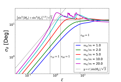
Figure 4: Spread in mutual inclination $\sigma_{\theta}$ (defined by Eqs. 27-28) between four planets in the presence of an external perturber ($m_{p}$) as a function of the coupling parameter $\bar{\epsilon}$ (defined by Eq. 29). The four planets are located at the semi-major axes $0.1,~{}0.15,~{}0.25,~{}0.4$ au, and are initially coplanar and inclined relative to the perturber at $\theta_{p}=10^{\circ}$. The dominant planet (the one with the largest mass, $m_{d}$) is the 4th planet (with the largest semi-major axis), and the other three planets have the same mass $m_{j}=m$. The different curves correspond to different mass ratio $m_{d}/m$, as indicated. The dimensionless parameter $\bar{\epsilon}$ is varied by varying the “strength” of the perturber, $m_{p}/a_{p}^{3}$. Analytical results in the strong coupling limit (Eq. 34) and weak coupling limit (Eq. 36), derived under the assumption $m_{d}/m\gg 1$, are also shown. Three resonance features are present when $m_{d}/m$ is sufficiently large. In the limit of $m_{d}/m\gg 1$ and $\theta_{p}\rightarrow 0$, these resonances are located at $\epsilon_{1d}=1$, $\epsilon_{2d}=1$ and $\epsilon_{3d}=1$.

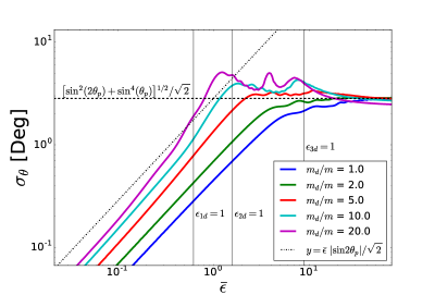
Figure 5: Same as Fig. 4, except for $\theta_{p}=2^{\circ}$.

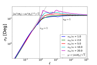
Figure 6: Same as Fig. 4, except that the third planet is the dominant planet.

To understand the numerical results shown in Fig. 4-6, we consider the limiting case of $m_{d}\gg m_{j}$ (with $j\neq d$). The angular momentum axis of the dominant planet precesses around $\bm{\hat{l}}_{p}$ with an approximately constant $\bm{\hat{l}}_{d}\cdot\bm{\hat{l}}_{p}=\cos\theta_{p}$. The sub-dominant planets are “shepherded” by $m_{d}$ in addition to the external perturber $m_{p}$.

In the strong coupling limit, with $|\epsilon_{jd}|\ll 1$, where

$$\epsilon_{jd}\equiv{\Omega_{dp}-\Omega_{jp}\over\omega_{jd}+\omega_{dj}},$$ (30)

we have (cf. Eq. 18)

$$\bm{\hat{l}}_{j}-\bm{\hat{l}}_{d}\simeq\epsilon_{jd}\cos\theta_{p}\Bigl{[}(1-\cos\tau_{jd})(\bm{\hat{l}}_{p}\!\times\!\bm{\hat{l}}_{d})\!\times\!\bm{\hat{l}}_{d}$$

$$\qquad\quad+\sin\tau_{jd}\,(\bm{\hat{l}}_{p}\!\times\!\bm{\hat{l}}_{d})\Bigr{]},$$ (31)

where $\tau_{jd}\equiv(\omega_{jd}+\omega_{dj})t$. Thus

$$\left|\sin\theta_{jd}\right|=\left|\bm{\hat{l}}_{j}\times\bm{\hat{l}}_{d}\right|\simeq\left|\epsilon_{jd}\sin 2\theta_{p}\sin{\tau_{jd}\over 2}\right|.$$ (32)

The misalignment spread of the $N$ planets is measured by

$${1\over N-1}\Bigl{\langle}\sum_{j}\bigl{|}\bm{\hat{l}}_{j}\times\bm{\hat{l}}_{d}\bigr{|}^{2}\Bigr{\rangle}\simeq{1\over 2(N-1)}\Bigl{(}\sum_{j}|\epsilon_{jd}|^{2}\Bigr{)}\sin^{2}\!2\theta_{p},$$ (33)

i.e.,

$${\rm RMS}\left(\sin\!\Delta\theta\right)\simeq{1\over\sqrt{2}}\,{\bar{\epsilon}}\,\left|\sin 2\theta_{p}\right|.$$ (34)

From Eq. (31), we also find

$$\langle\sin^{2}\!\theta_{jk}\rangle=\Bigl{\langle}|\bm{\hat{l}}_{j}\times\bm{\hat{l}}_{k}|^{2}\Bigr{\rangle}\simeq{\sin^{2}\!2\theta_{p}\over 2}\left(\epsilon_{jd}^{2}+\epsilon_{kd}^{2}-\epsilon_{jd}\epsilon_{kd}\right).$$ (35)

In Appendix B we present a more rigorous way to characterize the mutual inclination and the exact analytical expression in the strong coupling limit.

In the weak coupling limit, with $|\epsilon_{jd}|\gg 1$, all $\bm{\hat{l}}_{j}$’s precess independently around $\bm{\hat{l}}_{p}$. We have

$${\rm RMS}\left(\sin\!\Delta\theta\right)\simeq{1\over\sqrt{2}}\left(\sin^{2}\!2\theta_{p}+\sin^{4}\!\theta_{p}\right)^{1/2},$$ (36)

and

$$\left\langle\sin^{2}\!\theta_{jk}\right\rangle^{\!1/2}\simeq{1\over\sqrt{2}}\left(\sin^{2}\!2\theta_{p}+\sin^{4}\!\theta_{p}\right)^{1/2}.$$ (37)

Figures 4-reffig6 show that the numerical results match the analytical expressions in both strong and weak coupling limits. Resonance features also occur whenever a “minor” planet exists inside the dominant planet. The resonance is located at $\epsilon_{jd}\sim 1$ (with $a_{j}<a_{d}$).

Note that the small-scale non-smooth features seen in Figs. 4-6 are real, and likely result from the chaotic behavior the system due to the overlap of multiple nonlinear resonances. We will study this and other related issues in a future paper.

4 Summary and Discussion

4.1 Key Results

We have calculated the excitation of mutual inclinations in compact planetary systems by external planetary or stellar companions. Our key results are summarized in Figs. 2-6 and a number of approximate analytic expressions can be used to assess the importance of external perturbers of various masses ($m_{p}$), semi-major axis ($a_{p}$) and inclination ($\theta_{p}$). In general, the mutual inclination excited by a perturber depends on the dimensionless coupling parameter $\epsilon_{12}$ (Eq. 8 or 30), which measures the ratio of the differential precession rate of planet $1$ and $2$ induced by the perturber and their mutual precession rate. In order of magnitude, we have (Eq. 12)

$$\epsilon_{12}\sim\left({m_{p}\over m_{2}}\right)\left({a_{2}\over a_{p}}\right)^{3},$$ (38)

for $m_{2}\sim m_{1}$ and $a_{2}\mathrel{\raise 1.29167pt\hbox{$>$}\mkern-14.0mu\lower 2.58334pt\hbox{$\sim$}}a_{1}$.

For a two-planet system (see Fig. 2), the mutual inclination induced by an external companion is comparable to $\theta_{p}$ when $\epsilon_{12}\mathrel{\raise 1.29167pt\hbox{$>$}\mkern-14.0mu\lower 2.58334pt\hbox{$\sim$}}1$ (see Eqs. 23-24), but becomes $\sim\epsilon_{12}\theta_{p}$ when $\epsilon_{12}\mathrel{\raise 1.29167pt\hbox{$<$}\mkern-14.0mu\lower 2.58334pt\hbox{$\sim$}}1$ (see Eqs. 20-21). However, when $m_{2}\mathrel{\raise 1.29167pt\hbox{$>$}\mkern-14.0mu\lower 2.58334pt\hbox{$\sim$}}2m_{1}$ (i.e., the exterior planet is more massive), a resonance feature appears at around $\epsilon_{12}\sim 1$ where the mutual inclination may greatly exceed $\theta_{p}$ (see Fig. 3). This enhanced inclination excitation is the resulr of a secular nodal precession resonance (Appendix A).

The excitation of mutual inclinations in systems with more planets is necessarily more complex (Section 3 and Appendix B). Nevertheless, qualitative similar results can be obtained when the mutual inclination is measured relative to the more massive (“dominant”) planet in the system and when an averaged coupling parameter $\bar{\epsilon}$ is introduced (Eq. 29). Indeed, our approximate analytic expressions for the mutual inclination spread (Eq. 34 in the strong coupling limit and Eq. 36 in the weak coupling limit) are in agreement with the numerical results (see Figs. 4-6).

4.2 Applications to Individual Systems

As noted in Section 1, a number of “inner planets + companion” systems have been observed. Here we discuss some of these systems in light of our theoretical results.

Kepler-68 ($M_{\star}=1.08M_{\odot},~{}R_{\star}=1.24R_{\odot}$) has two transiting planets ($m_{1,2}=8.3,~{}4.8M_{\oplus}$) at $a_{1,2}=0.0617,~{}0.0906$ au, and a non-transiting giant planet $m_{p}\mathrel{\raise 1.29167pt\hbox{$>$}\mkern-14.0mu\lower 2.58334pt\hbox{$\sim$}}0.95M_{J}$ at $a_{p}=1.4$ au ($e_{p}=0.18$) (Gilliland et al. 2013). The coupling parameter is $\epsilon_{12}\simeq 2.3\times 10^{-3}$ using the lower limit for $m_{p}$. The excited mutual inclination spread of the two inner planet is $\sigma_{\theta}=\epsilon_{12}\sin 2\theta_{p}/\sqrt{2}\mathrel{\raise 1.29167pt\hbox{$<$}\mkern-14.0mu\lower 2.58334pt\hbox{$\sim$}}0.14^{\circ}$ (regardless of $\theta_{p}$), and is smaller than $R_{\star}/a_{2}=3.6^{\circ}$, consistent with the coplanarity of the two inner planets.

Kepler-48 ($M_{\star}=0.88M_{\odot}$, $R_{\star}=0.89R_{\odot}$) has three transiting inner planets ($m_{1,2,3}=0.0124,\,0.046,\,0.015M_{J}$) at $a_{1,2,3}=0.053,\,0.085,\,0.23$ au, and a giant planet ($m_{p}\mathrel{\raise 1.29167pt\hbox{$>$}\mkern-14.0mu\lower 2.58334pt\hbox{$\sim$}}2.1M_{J}$) at $a_{p}=1.85$ au ($982$ days) (Marcy et al. 2014). The coupling parameters are $\epsilon_{12}\simeq 0.0015$ and $\epsilon_{23}\simeq 0.25$ using $m_{p}=2.1M_{J}$. Significant mutual inclination can be excited between planet 2 and 3 if $\theta_{p}$ is large. Requiring $\theta_{23}\sim\epsilon_{23}\theta_{p}\mathrel{\raise 1.29167pt\hbox{$<$}\mkern-14.0mu\lower 2.58334pt\hbox{$\sim$}}R_{\star}/a_{3}=1.03^{\circ}$ yields $\theta_{p}\mathrel{\raise 1.29167pt\hbox{$<$}\mkern-14.0mu\lower 2.58334pt\hbox{$\sim$}}2.3^{\circ}$. We therefore predict that the non-transiting planet (Kepler-48e) is closely aligned with the inner transiting planets. Note that since $R_{\star}/a_{p}=0.13^{\circ}$, its transit probability is still small.

Kepler-56 (with a red giant host star $M_{\star}=1.32M_{\odot}$, $R_{\star}=4.23R_{\odot}$) has two transiting planets ($m_{1,2}=0.0695,\,0.57M_{J}$) at $a_{1,2}=0.103,\,0.165$ au (period $10.5,\,21$ days). The orbits of the two planets are coplanar within $\sim R_{\star}/a_{2}=6.8^{\circ}$, and are inclined with respect to the stellar equator by more than $37^{\circ}$ (Huber et al. 2013). RV observations reveal a third planet with period 1002 days ($a_{p}=2.16$ au), $e_{p}=0.2$, and $m_{p}\geq 5.6M_{J}$ (Oter et al. 2016). This implies a coupling parameter of $\epsilon_{12}\geq 1.6\times 10^{-3}$. Thus the inner two planets are strongly coupled and their coplanarity is not affected by any (regardless of $\theta_{p}$) external perturbers that satisfy the current RV constraint. However, the observed large stellar obliquity may require a large $\theta_{p}$.

WASP-47 ($M_{\star}=1.04M_{\odot}$) contains three transiting planets (Becker et al. 2015; Dai et al. 2015): a hot Jupiter ($1.16M_{J}$, $a_{2}=0.051$ au or 4.16 days) with an inner super-Earth ($1.8R_{\oplus}$ or $12M_{\oplus}$, 0.79 days) and an outer Neptune-size planet ($3.6R_{\oplus}$ or $10.4\pm 8.4M_{\oplus}$, 9.03 days). These inner planets are orbited by an external giant planet ($m_{p}>1.24M_{J}$) with $e=0.13$ and $P=572$ days (Neveu-VanMalle et al. 2016). The inner planets are well in the strong coupling regime, with $|\epsilon_{jk}|\ll 1$ ($\epsilon_{12}=2\times 10^{-4}$ and $\epsilon_{23}=1.7\times 10^{-4}$).

Kepler-454 ($M_{\star}=1.03M_{\odot}$) has a 10.6 day ($a_{1}=0.095$ au) transiting planet ($2.37R_{E}$, 6.84$M_{\oplus}$), a cold Jupiter ($m_{p}>4.46M_{J}$ at 524 days) and a distant companion ($>$12$M_{J}$ at $>$10 years) (Gettel et al. 2016). The observed system has $\epsilon=(m_{p}/m_{1})(a_{1}/a_{p})^{3}\sim 0.1(m_{p}/5M_{J})$. A neighboring planet $m_{2}\sim m_{1}$ would give $\epsilon_{12}\sim(a_{2}/0.2~{}{\rm au})^{3}(m_{p}/5M_{J})$, and would be easily inclined relative to $m_{1}$ and not observable. Thus Kepler-454 could be an example of multi-planet systems that haven been “disrupted” by giant planet perturbers.

GJ 832 ($M_{\star}=0.832M_{\odot}$) has a super Earth ($m_{1}>5.4M_{\oplus}$ at $0.162$ au) inside a giant planet ($m_{p}>0.64M_{J}$ at $3.4$ au), both discovered by RV (Wittenmyer et al. 2014). With $\epsilon=(m_{p}/m_{1})(a_{1}/a_{p})^{3}\sim 0.006(m_{p}/M_{J})(m_{1}/6M_{\oplus})^{-1}$, any neighboring planet to $m_{1}$ is strongly coupled to it.

55 Cancri ($M_{\star}=0.95M_{\odot}$) has four inner planets (e,b,c,f) with $m_{e,b}\simeq 0.027,~{}0.83M_{J}$, $m_{c}>0.17M_{J}$, $m_{f}>0.16M_{J}$ at $0.0156,~{}0.115,~{}0.24,~{}0.78$ au, and an external giant planet (d) with $m_{d}>3.8M_{J}$ and $a_{d}=5.74$ au (Dawson & Fabrycky 2010). The outer planet may be inclined with respect to the line of sight by $\sim 53^{\circ}$ (McArthur et al. 2004), implying $\theta_{p}\mathrel{\raise 1.29167pt\hbox{$>$}\mkern-14.0mu\lower 2.58334pt\hbox{$\sim$}}37^{\circ}$ relative to planet e. Since $\epsilon=(m_{d}/m_{f})(a_{f}/a_{d})^{3}\sim 0.08(m_{d}/5M_{J})(m_{f}/0.16M_{J})^{-1}$, planet d, even if highly misaligned, cannot significantly influence the coplanarity of the inner planets. The planetary system is also orbited by a distant stellar companion 55 Cnc B at $a_{B}\sim 1065$ au (projected distance). But this will not perturb the coplanarity of the planets since $(M_{B}/m_{d})(a_{d}/a_{B})^{3}\ll 1$.

Kepler-444 ($M_{\star}=0.76M_{\odot}$) has five sub-Earth radius planets (0.40 - 0.74$R_{\oplus}$) at semi-major axes $0.0418,~{}0.0488,~{}0.06,~{}0.0696,~{}0.0811$ au (Campante et al. 2015) orbiting the primary star (Kepler-444A). Astrometric and RV observations show that a pair of M dwarfs (BC) with total mass $m_{p}\equiv m_{BC}=0.54M_{\odot}$ orbits around Kepler-444A with semi-major axis $a_{p}\simeq 37$ au and eccentricity $e_{p}=0.864$ (Dupuy et al. 2016). Both the planetary system and the A-BC binary have edge-on orbits relative to the line of sight. Using $m_{5}\sim 0.54M_{\oplus}$ [from the planet mass-radius relation $m/M_{\oplus}\simeq(R/R_{\oplus})^{2.06}$], we find the coupling parameter $\epsilon\sim(m_{BC}/m_{5})\left(a_{5}/a_{p}\sqrt{1-e_{p}^{2}}\right)^{3}\sim 0.026$, and thus the five planets are strongly coupled and can maintain their coplanarity (in agreement with the numerical simulation of Dupuy et al. 2016).

4.3 Implications for Kepler Dichotomy

The common occurrence of giant planets and stellar companions outside compact planetary systems (see Sections 1 and 4.2) suggests that these giant planets or more massive distant stellar perturbers can excite mutual inclinations in the inner planets, thereby account for an appreciable fraction of the Kepler “singles”. Our work provides a quantitative criterion (in terms of the strength of the perturber, $m_{p}/a_{p}^{3}$) for inclination excitations. Continued search for external companions of inner transiting planets would help constrain various scenarios (see Section 1) for producing the Kepler dichotomy.

As noted in Section 1, inclined stellar companions may be a natural consequence of the binary formation process, while inclined giant planets may be produced by strong planet-planet scatterings. In the latter case, the inner multi-planet system may experience some excitation of mutual inclinations while the outer giant planets undergo scatterings. (Of course, if the inner planets are not well separated from the outer giants, they may be completely disrupted.) Our numerical calculations (Pu & Lai 2016, in prep) suggest that in many cases, the mutual inclination excitation in the inner system during the outer-planet scattering phase is smaller than the subsequent secular phase.

In this paper we have focused on the excitation of mutual inclinations, since they most directly influence the transit probability of multiple planets. Eccentricities are also excited by external companions (Pu & Lai 2016, in prep). This may explain why Kepler “singles” (or a fraction of them) are more eccentric than the Kepler “multis”, for which the exists tentative observational evidence (J. Xie et al. 2016).

While Kepler single-transit systems may contain other planets hidden from transit observations due to mutual inclinations, it is also possible that they are true “singles” because of the dynamical influences of external giant planets. For example, when appreciable mutual inclinations and eccentricities are excited, the inner planetary systems are likely more unstable and will suffer self-destruction (e.g. Veras & Armitage 2004; Pu & Wu 2015). In addition, as noted above, the inner planetary systems could have been severely disrupted while strong planet scatterings took place at a few au’s that produced inclined/eccentric giant planets. Continued search for close neighbors of single-transit planets would shed light on this issue.

Appendix A Hamiltonian Theory for Resonance

We consider a system with a “dominant” planet (labeled “d”) whose mass and angular momentum are much larger than the other planets ($m_{d}\gg m_{j}$ and $L_{d}\gg L_{j}$, with $j\neq d$). The Hamiltonian governing the dynamics of $\bm{\hat{l}}_{j}(t)$ is

$$H=-{1\over 2}\,\omega_{jd}\,L_{j}\,(\bm{\hat{l}}_{j}\cdot\bm{\hat{l}}_{d})^{2}-{1\over 2}\,\Omega_{jp}\,L_{j}\,(\bm{\hat{l}}_{j}\cdot\bm{\hat{l}}_{p})^{2},$$ (A1)

where we have neglected a non-essential additive constant. Since $m_{d}$ is the dominant planet, its $\bm{\hat{l}}_{d}$ simply precesses around $\bm{\hat{l}}_{p}$ with a constant rate, $-\Omega_{dp}\,(\bm{\hat{l}}_{d}\cdot\bm{\hat{l}}_{p})\simeq-\Omega_{dp}\cos\!\theta_{p}$:

$${\text{d}\bm{\hat{l}}_{d}\over\text{d}t}\simeq-\Omega_{dp}(\bm{\hat{l}}_{d}\cdot\bm{\hat{l}}_{p})\,\bm{\hat{l}}_{p}\times\bm{\hat{l}}_{d}.$$ (A2)

In the frame corotating with $\bm{\hat{l}}_{d}$, the Hamiltonian (A1) transforms to

$$H_{\rm rot}\simeq H+\Omega_{dp}\,(\bm{\hat{l}}_{d}\cdot\bm{\hat{l}}_{p})\,\bm{\hat{l}}_{p}\cdot(L_{j}\bm{\hat{l}}_{j}).$$ (A3)

It is convenient to use the rescaled Hamiltonian,

$${\tilde{H}}_{\rm rot}={H_{\rm rot}\over L_{j}}\simeq-{1\over 2}\,\omega_{jd}\,\cos^{2}\!\theta_{jd}-{1\over 2}\,\Omega_{jp}\,(\bm{\hat{l}}_{j}\cdot\bm{\hat{l}}_{p})^{2}$$

$$\qquad\qquad\quad+\Omega_{dp}\cos\!\theta_{p}\,(\bm{\hat{l}}_{j}\cdot\bm{\hat{l}}_{p}),$$ (A4)

where

$$\bm{\hat{l}}_{j}\cdot\bm{\hat{l}}_{p}=\sin\theta_{p}\sin\theta_{jd}\cos\varphi_{jd}+\cos\theta_{p}\cos\theta_{jd}.$$ (A5)

Here $\theta_{jd}$ and $\varphi_{jd}$ are the polar angle and azimuthal angle of $\bm{\hat{l}}_{j}$ measured relative to $\bm{\hat{l}}_{d}$ (i.e., $\cos\theta_{jd}=\bm{\hat{l}}_{j}\cdot\bm{\hat{l}}_{d}$). Note that $\varphi_{jd}$ and $\cos\theta_{jd}$ form the conjugate coordinate and momentum for the Hamiltonian ${\tilde{H}}_{\rm rot}$.

Suppose $\theta_{jd}=0$ at $t=0$. Then the phase-space curve for the evolution of $\cos\theta_{jd}$ and $\varphi_{jd}$ is determined by

$$-{1\over 2}\,\hat{\Omega}_{jp}\,(\bm{\hat{l}}_{j}\cdot\bm{\hat{l}}_{p})^{2}+\hat{\Omega}_{dp}\cos\theta_{p}\,(\bm{\hat{l}}_{j}\cdot\bm{\hat{l}}_{p})+{1\over 2}\,\sin^{2}\!\theta_{jd}$$

$$\qquad\qquad\simeq\Bigl{(}\hat{\Omega}_{dp}-{1\over 2}\hat{\Omega}_{jp}\Bigr{)}\cos^{2}\!\theta_{p},$$ (A6)

where

$$\hat{\Omega}_{jp}\equiv{\Omega_{jp}\over\omega_{jd}},\quad\hat{\Omega}_{dp}\equiv{\Omega_{dp}\over\omega_{jd}}.$$ (A7)

The maximum value $\theta_{m}\equiv(\theta_{jd})_{\rm max}$ is achieved at $\varphi_{jd}=0$ or $\pi$, and is given by

$$-{1\over 2}\,\hat{\Omega}_{jp}\,\cos^{2}(\theta_{m}\mp\theta_{p})+\hat{\Omega}_{dp}\cos\theta_{p}\,\cos(\theta_{m}\mp\theta_{p})$$

$$\qquad+{1\over 2}\,\sin^{2}\!\theta_{m}\simeq\Bigl{(}\hat{\Omega}_{dp}-{1\over 2}\hat{\Omega}_{jp}\Bigr{)}\cos^{2}\!\theta_{p},$$ (A8)

where the upper (lower) sign is for $\varphi_{jd}=0$ ($\pi$).

Figures 7 and 8 show some example phase-space curves for the cases of $a_{d}>a_{j}$ and $a_{d}<a_{j}$, respectively. These two cases have very different phase-space structure, with the former showing clear resonance feature.

Equation (A8) can be solved analytically in several limiting cases:

(i) In the strong coupling limit (but general $\theta_{p}$), $\hat{\Omega}_{jp},\hat{\Omega}_{dp}\ll 1$, we expect $\theta_{m}\ll 1$. Expanding Eq. (A8) for small $\theta_{m}$, we find

$$\theta_{m}\simeq\mp\epsilon_{jd}\sin 2\theta_{p},\qquad{\rm i.e.,}~{}~{}\theta_{m}\simeq|\epsilon_{jd}\sin 2\theta_{p}|,$$ (A9)

in agreement with Eq. (20).

(ii) In the weak coupling limit (but general $\theta_{p}$), $\hat{\Omega}_{jp},\hat{\Omega}_{dp}\gg 1$, Eq. (A8) has the solution (see Eq. 23)

$$\theta_{m}\simeq 2\theta_{p}\qquad({\rm with}~{}~{}\varphi_{jd}=0).$$ (A10)

(iii) In the singular limit of $\theta_{p}=0$, Eq. (A8) has two roots: The first root is $\theta_{m}=0$. The second root is

$$\cos\theta_{m}={2\hat{\Omega}_{dp}\over 1+\hat{\Omega}_{jp}}-1,\qquad({\rm 2nd~{}root})$$ (A11)

which exists only when $|\cos\theta_{m}|<1$, or $\epsilon_{jd}=\hat{\Omega}_{dp}-\hat{\Omega}_{jp}<1$.

(iv) In the limit of $\theta_{p}\ll 1$ (but general $\epsilon_{jd}$), the second root (Eq. A11) remains valid provided that $\theta_{m}\gg\theta_{p}$:

$$\cos\theta_{m}\simeq{2\hat{\Omega}_{dp}\over 1+\hat{\Omega}_{jp}}-1,\qquad({\rm 2nd~{}root;valid~{}for}~{}\theta_{m}\gg\theta_{p})$$ (A12)

This root (which exists only when $\epsilon_{jd}=\hat{\Omega}_{dp}-\hat{\Omega}_{jp}\mathrel{\raise 1.29167pt\hbox{$<$}\mkern-14.0mu\lower 2.58334pt\hbox{$\sim$}}1$) cannot be reached for systems with initially aligned inner planets ($\theta_{jd}=0$) (see Figs. 7 and 8). The correction to the first root ($\theta_{m}=0$ in the limit of $\theta_{p}=0$) due to finite (but small) $\theta_{p}$ can be obtained by expanding Eq. (A8) for $\theta_{p},\theta_{m}\ll 1$. We find

$$\theta_{m}\simeq\pm\,{2\epsilon_{jd}\theta_{p}\over\epsilon_{jd}-1}\qquad({\rm for~{}general}~{}\epsilon_{dj},~{}{\rm but}~{}\theta_{p},\theta_{m}\ll 1)$$ (A13)

(recall that the upper/lower sign is for $\varphi_{jd}=0,\pi$). Clearly, Eq. (A13) reduces to (A9) and (A10) in the appropriate limits. Most importantly, Eq. (A13) shows that a sharp resonance occurs when

$$\epsilon_{jd}={\Omega_{dp}-\Omega_{jp}\over\omega_{jd}}=1.$$ (A14)

At the resonance, $\theta_{m}\gg\theta_{p}$ can be attained (but note that Eq. A13 breaks down for $\epsilon_{jd}\rightarrow 1$). Clearly, the resonance condition can be realized only if $a_{d}>a_{j}$ (i.e, the dominant planet is outside the “minor” one). Note that Eq. (A14) is exact only in the limit of $\theta_{p}\rightarrow 0$ and $m_{d}\gg m_{j}$; otherwise the resonance is shifted and broadened (see Figs. 2-6).

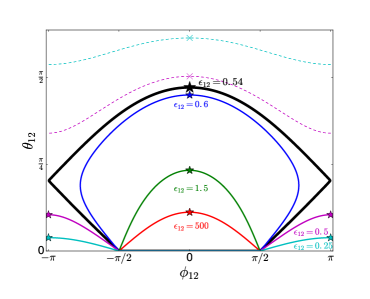
Figure 7: Phase-space curves for the mutual inclination of a two-planet system with an external perturber. The two planets have $a_{1}=0.3$ au and $a_{2}=0.5$ au, with masses $m_{2}\gg m_{1}$, and the perturber’s orbit is inclined at $\theta_{p}=10^{\circ}$. The different curves correspond to different values of $\epsilon_{12}$, as indicated; the solid curves can be reached by an initially aligned system ($\theta_{12}=0$), while the dashed curves are unreachable. The maximum $\theta_{12}$ for each value of $\epsilon_{12}$ is marked. The thick solid line is the separatrix (corresponding to a critical value of $\epsilon_{12}$) at which $(\theta_{12}){\rm max}$ experiences a sudden jump (see Fig. 3).

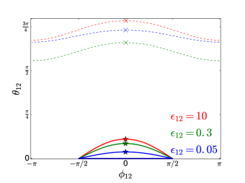
Figure 8: Same as Fig. 7 except for $m_{2}\ll m_{1}$.

Appendix B General Equations for Multi-Planet Systems

The result of Section 2 can be easily generalized to a system with $N$ inner planets with an inclined external perturber $m_{p}$. The evolution of $\bm{\hat{l}}_{j}$ ($j=1,2,\cdots,N$) is governed by the equation

$${\text{d}\bm{\hat{l}}_{j}\over\text{d}t}=\sum_{k\neq j}\omega_{jk}(\bm{\hat{l}}_{j}\cdot\bm{\hat{l}}_{k})(\bm{\hat{l}}_{j}\times\bm{\hat{l}}_{k})+\Omega_{jp}(\bm{\hat{l}}_{j}\cdot\bm{\hat{l}}_{p})(\bm{\hat{l}}_{j}\times\bm{\hat{l}}_{p}),$$ (B1)

where

$$\omega_{jk}={Gm_{j}m_{k}a_{<}\over 4a_{>}^{2}L_{j}}b_{3/2}^{(1)}\!\left({a_{<}\over a_{>}}\right),$$ (B2)

$$\Omega_{jp}={Gm_{j}m_{p}a_{j}\over 4a_{p}^{2}L_{j}}b_{3/2}^{(1)}\!\left({a_{j}\over a_{p}}\right),$$ (B3)

with $a_{<}\equiv\min(a_{j},a_{k})$ and $a_{>}\equiv\max(a_{j},a_{k})$.

In the strong-coupling limit, with $|\bm{\hat{l}}_{j}-\bm{\hat{l}}_{k}|\ll 1$, the total angular momentum of the inner binary, $\bm{L}=L\,\bm{\hat{l}}=\sum_{j}\bm{L}_{j}$, evolves according to Eq. (13), with the precession rate given by

$$\Omega_{L}\simeq{1\over L}\sum_{j}L_{j}\Omega_{jp}.$$ (B4)

In the corotating frame of $\bm{L}$, the evolution of $\Delta{\bm{l}}_{j}=\bm{\hat{l}}_{j}-\bm{\hat{l}}$ is governed by the equation

$$\biggl{(}{\text{d}\Delta{\bm{l}}_{j}\over\text{d}t}\biggr{)}_{\rm rot}\simeq-\sum_{k\neq j}\omega_{jk}\bm{\hat{l}}\times(\Delta{\bm{l}}_{j}-\Delta{\bm{l}}_{k})$$

$$\qquad\qquad\quad+(\Omega_{jp}-\Omega_{L})(\bm{\hat{l}}\cdot\bm{\hat{l}}_{p})(\bm{\hat{l}}\times\bm{\hat{l}}_{p}).$$ (B5)

We can recast Eq. (B5) into a more convenient form. Set up a Cartesian coordinate system, with the $z$-axis along $\bm{\hat{l}}$ and the $y$-axis along $\bm{\hat{l}}\times\bm{\hat{l}}_{p}$. Let $\Delta{\bm{l}}_{j}=(\Delta l_{j})_{x}{\bm{\hat{x}}}+(\Delta l_{j})_{y}{\bm{\hat{y}}}$, and define the complex variable

$$I_{j}\equiv(\Delta l_{j})_{x}+i(\Delta l_{j})_{y}.$$ (B6)

Then Eq. (B5) reduces to (suppressing the subscript “rot”)

$${\text{d}I_{j}\over\text{d}t}=-i\sum_{k}A_{jk}I_{k}+iB_{j},$$ (B7)

where

$$A_{jk}=\Bigl{(}\sum_{n}\omega_{jn}\Bigr{)}\delta_{jk}-\omega_{jk},$$ (B8)

$$B_{j}=(\Omega_{jp}-\Omega_{L})\sin\theta_{p}\cos\theta_{p}.$$ (B9)

We can write Eq. (B7) in a more compact form:

$${\text{d}\bm{Y}\over\text{d}t}=-i\bm{A}\cdot\bm{Y}+i\bm{B},$$ (B10)

where the $N\times N$ matrix has the element $A_{jk}$, and

$$\bm{Y}=\left(\begin{array}[]{c}I_{1}\\ I_{2}\\ \vdots\\ I_{N}\end{array}\right),\quad\bm{B}=\left(\begin{array}[]{c}B_{1}\\ B_{2}\\ \vdots\\ B_{N}\end{array}\right).$$ (B11)

In the absence of the external perturber, $B_{j}=0$, Eq. (B7) or (B10) describes the free inclination oscillations of the $N$-planet system (Murray & Dermott 1999). The eigenmodes $\bm{Y}_{\alpha}$ ($\alpha=1,2,\cdots,N$) of these free oscillations satisfy the equation

$$\lambda_{\alpha}\bm{Y}_{\alpha}=\bm{A}\cdot\bm{Y}_{\alpha},$$ (B12)

where $\lambda_{\alpha}$ is the eigenvalue, with $\bm{Y}_{\alpha}\propto\exp(-i\lambda_{\alpha}t)$.

The general solution of Eq. (B10) takes the form

$$\bm{Y}(t)=\bm{A}^{-1}\!\cdot\!\bm{B}+\sum_{\alpha}c_{\alpha}\bm{Y}_{\alpha}\exp(-i\lambda_{\alpha}t),$$ (B13)

where the constants $c_{\alpha}$’s are determined by the initial condition. Assuming $\bm{Y}(t=0)=0$, we have

$$c_{\alpha}=-\bm{Y}_{\alpha}^{\dagger}\!\cdot\!\bm{A}^{-1}\!\cdot\!\bm{B},$$ (B14)

where the eigenvector $\bm{Y}_{\alpha}$ has been normalized by

$$\bm{Y}_{\alpha}^{\dagger}\!\cdot\!\bm{Y}_{\beta}=\delta_{\alpha\beta}.$$ (B15)

The mutual inclination in the $N$-planet system is measured by

$${1\over N}\sum_{j}\bigl{|}\bm{\hat{l}}_{j}\times\bm{\hat{l}}\bigr{|}^{2}={1\over N}\sum_{j}|I_{j}(t)|^{2}={1\over N}\Bigl{|}\bm{Y}(t)\Bigr{|}^{2}.$$ (B16)

Using Eq. (B13), we then have

$$\left\langle{1\over N}\sum_{j}\bigl{|}\bm{\hat{l}}_{j}\times\bm{\hat{l}}\bigr{|}^{2}\right\rangle={1\over N}\Bigl{[}\bigl{|}\bm{A}^{-1}\!\cdot\!\bm{B}\bigr{|}^{2}+\sum_{\alpha}|c_{\alpha}|^{2}\Bigr{]}.$$ (B17)

References

- Bate (2009) Albrecht, S., et al. 2013, ApJ, 771, 11
- Bate (2009) Ballard, S., Johnson, J.A. 2016, ApJ, 816, 66
- Bate (2009) Baranec, C., et al. 2016, AJ, 152, 18
- Bate (2009) Becker, J.C., Adams, F.C. 2016, MNRAS, 455, 2980
- Bate (2009) Becker, J.C., et al. 2015, ApJ, 812, L18
- Bate (2009) Boue, G., Fabrycky, D.C. 2014, ApJ, 789, 110
- Bate (2009) Bryan, M., et al. 2016, ApJ, 821, 89
- Bate (2009) Campante, T.L., et al. 2015, ApJ, 799, 170
- Bate (2009) Chatterjee, S., Ford, E.B., Matsumura, S., Rasio, F.A. 2008, ApJ, 686, 580,
- Bate (2009) Coughlin, J.L., et al. 2016, ApJS, 224, 12
- Bate (2009) Cumming, A., et al. 2008, PASP, 120, 531
- Bate (2009) Dai, F., et al. 2015, ApJ, 813, L9
- Bate (2009) Dawson, R.I., Fabrycky, D.C. 2010, ApJ, 722, 937
- Bate (2009) Dupuy, T.J., et al. 2016, ApJ, 817, 80
- Bate (2009) Fabrycky, D.C., et al. 2014, ApJ, 790, 146
- Bate (2009) Fang, J., Margot, J.-L. 2012, ApJ, 761, 92
- Bate (2009) Fang, J., Margot, J.-L. 2013, ApJ, 767, 115
- Bate (2009) Feng, Y.K., et al. 2015, ApJ, 800, 22
- Bate (2009) Figueira, P., et al. 2012, A&A, 541, A139
- Bate (2009) Foucart, F., Lai, D. 2011, MNRAS, 412, 2799
- Bate (2009) Foucart, F., Lai, D. 2014, MNRAS, 445, 173
- Bate (2009) Gettel, S., et al. 2016, ApJ, 816, 95
- Bate (2009) Gilliland, R.L. et al. 2013, ApJ, 766, 40
- Bate (2009) Hale, A. 1994, AJ, 107, 306
- Bate (2009) Hansen, B.M.S, & Murray, N. 2013, ApJ, 775, 53
- Bate (2009) Huber, D., et al. 2013, Science, 342, 331
- Bate (2009) Johansen, A., Davies, M.B., Church, R.P., Holmelin, V. 2012, ApJ, 758, 39
- Bate (2009) Juric, M., Tremaine, S. 2008, ApJ, 686, 603
- Bate (2009) Kraus, A.L., et al. 2016, AJ, 152, 8
- Bate (2009) Lai, D. 2014, MNRAS, 440, 3532
- Bate (2009) Lissauer, J.J., et al. 2011, ApJS, 197, 8
- Bate (2009) Liu, B., Munoz, D.J., Lai, D. 2015, MNRAS, 447, 747
- Bate (2009) Marcy, G.W., et al. 2014, ApJ, 210, 20
- Bate (2009) Marmier, M., et al. 2013, A&A, 551, 90
- Bate (2009) McArthur, B.E., et al. 2004, ApJ, 614, L81
- Bate (2009) Moriarty, J., Ballard, S. 2015, arXiv:1512.03445
- Bate (2009) Morton, T.D., et al. 2016, ApJ, 822, 86
- Bate (2009) Morton, T.D., Winn, J.N. 2014, ApJ, 796, 47
- Bate (2009) Moutou, C., et al. 2015, A&A, 576, 48
- Bate (2009) Mullally, F., et al. 2015, ApJS, 217, 31
- Bate (2009) Murray, C.D., Dermott, S.F. 1999, Solar System Dynamics (Cambridge Univ. Press)
- Bate (2009) Neveu-VanMalle, M., et al. 2016, A&A, 586, 92
- Bate (2009) Ngo, H., et al. 2016, ApJ, in press (arXiv:1606.07102)
- Bate (2009) Oter, O.J., et al. 2016, arXiv:1608.03627
- Bate (2009) Pu, B., Wu, Y. 2015, ApJ, 807, 44
- Bate (2009) Rowan, D., et al. 2016, ApJ, 817, 104
- Bate (2009) Schmitt, J.R., et al. 2014, AJ, 148, 28
- Bate (2009) Tremaine S. 1991, Icarus, 89, 85
- Bate (2009) Tremaine S., Dong, S. 2012, AJ, 143, 94
- Bate (2009) Tremaine S., Touma J., Namouni F., 2009, AJ, 137, 3706
- Bate (2009) Uehara, S., et al. 2016, ApJ, 822, 2
- Bate (2009) Veras, D., Armitage, P.J. 2004, Icarus, 172, 349
- Bate (2009) Volk, K., Gladman, B. 2015, ApJ, 806, L26
- Bate (2009) Wang, J., Fischer, D.A., Horch, E.P., Xie, J.-W. 2015a, ApJ, 806, 248
- Bate (2009) Wang, J., Fischer, D.A., Xie, J.-W., Ciardi, D.R. 2015b, ApJ, 813, 130
- Bate (2009) Weissbein, A., Steinberg, E., Sari, R. 2012, arXiv:1203.6072
- Bate (2009) Wittenmyer, R.A., et al. 2014, 791, 114
- Bate (2009) Wittenmyer, R.A., et al. 2016, ApJ, 819, 28
- Bate (2009) Xie, J.-W., Wu, Y., Lithwick, Y. 2014, ApJ, 789, 165
- Bate (2009) Xie, J.-W., et al. 2016, arXiv:1609.08633