The LPM effect in sequential bremsstrahlung:
dimensional regularization

Abstract

The splitting processes of bremsstrahlung and pair production in a medium are coherent over large distances in the very high energy limit, which leads to a suppression known as the Landau-Pomeranchuk-Migdal (LPM) effect. Of recent interest is the case when the coherence lengths of two consecutive splitting processes overlap (which is important for understanding corrections to standard treatments of the LPM effect in QCD). In previous papers, we have developed methods for computing such corrections without making soft-gluon approximations. However, our methods require consistent treatment of canceling ultraviolet (UV) divergences associated with coincident emission times, even for processes with tree-level amplitudes. In this paper, we show how to use dimensional regularization to properly handle the UV contributions. We also present a simple diagnostic test that any consistent UV regularization method for this problem needs to pass.

I Introduction

When passing through matter, high energy particles lose energy by showering, via the splitting processes of hard bremsstrahlung and pair production. At very high energy, the quantum mechanical duration of each splitting process, known as the formation time, exceeds the mean free time for collisions with the medium, leading to a significant reduction in the splitting rate known as the Landau-Pomeranchuk-Migdal (LPM) effect LP ; Migdal . As we will review shortly, calculations of the LPM effect must typically deal with ultraviolet (UV) divergences in intermediate steps, associated with effectively-vacuum evolution between nearly coincident times. For the case of computing single splitting rates, these divergences are trivial to deal with (either by subtracting out the vacuum rate a priori, or by using an appropriate $i\epsilon$ prescription). However, for the case of two consecutive splittings with overlapping formation times (which we will loosely characterize as “double bremsstrahlung”), the treatment of ultraviolet divergences is much more difficult. In previous work 2brem , an $i\epsilon$ prescription was proposed for dealing with this problem. Here, we will explain why that prescription was incomplete and missed certain contributions to the result. Then we will show how to correctly regulate the ultraviolet using dimensional regularization and will use our results to correct the QCD LPM analysis of ref. 2brem . In addition, we provide a simple example—QED double bremsstrahlung in an independent emission approximation—that can be used as a test of the self-consistency of UV regularization prescriptions.

For simplicity of discussion, and in order to make contact with the double bremsstrahlung calculation of refs. 2brem ; seq , we will restrict attention in this paper to the case of medium-induced bremsstrahlung from an (approximately) on-shell particle traversing a thick, uniform medium in the multiple scattering ($\hat{q}$) approximation. (Thick means large compared to the formation time of the bremsstrahlung radiation.) However, the same methods should be useful for double bremsstrahlung in other situations.

I.1 Examples of UV divergences

I.1.1 Single splitting

The standard result for the single splitting rate in a thick, uniform medium in multiple scattering approximation is BDMS

$$\frac{d\Gamma}{dx}=-\frac{\alpha P(x)}{\pi}\operatorname{Re}\int_{0}^{\infty}d(\Delta t)\>\Omega^{2}\csc^{2}(\Omega\,\Delta t),$$ (1)

where $x$ is the momentum fraction of one of the daughters, and $P(x)$ is the corresponding (vacuum) Dokshitzer-Gribov-Lipatov-Altarelli-Parisi (DGLAP) splitting function. $\Delta t$ represents the time between emission in the amplitude and emission in the conjugate amplitude, as depicted in fig. 1. $\Omega$ is a complex frequency that characterizes the evolution and decoherence of this interference contribution with time $\Delta t$. In the QCD case of $g\to gg$, for example, it is given by

$$\Omega=\sqrt{-\frac{i\hat{q}_{\rm A}}{2E}\left(-1+\frac{1}{1{-}x}+\frac{1}{x}\right)},$$ (2)

where $\hat{q}$ characterizes transverse momentum diffusion of a high-energy particle due to interactions with the medium (average $Q_{\perp}^{2}=\hat{q}t$) and $\hat{q}_{\rm A}$ indicates $\hat{q}$ for an adjoint-color particle, i.e. a gluon. $E$ is the initial particle energy. Throughout this paper, we will focus on splitting rates that have been integrated over the final transverse momenta of the (nearly collinear) daughters.

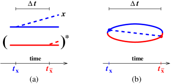
Figure 1: (a) Interference contribution corresponding to the single bremsstrahlung rate, and (b) an equivalent diagrammatic representation, where the amplitude (blue) and conjugate amplitude (red) are drawn sewn together. To simplify the drawing, all particles, including gluons, are indicated by straight lines. Only the high-energy parent and its two daughters are shown explicitly; the multiple interactions of these particles with the medium are implicit and not shown.

The negative imaginary part of $\Omega$ accounts for decoherence of interference (such as fig. 1) at large time separation, due to random interactions with the medium. In particular, the integrand in (1) falls exponentially for $|\Omega|\,\Delta t\gg 1$, and so the integral is infrared ($\Delta t{\to}\infty$) convergent.

The details of the above formulas are not important yet. What is important is the behavior of the integrand in (1) as $\Delta t\to 0$:

$$\frac{d\Gamma}{dx}\to-\frac{\alpha P(x)}{\pi}\operatorname{Re}\int_{0}d(\Delta t)\left[\frac{1}{(\Delta t)^{2}}+O\bigl{(}(\Delta t)^{0}\bigr{)}\right],$$ (3)

which makes the integral UV divergent. Note that this divergence does not depend on the medium parameter $\hat{q}$ and so represents a purely vacuum contribution to the rate. One way to deal with it is to note that an on-shell particle cannot split in vacuum, and so the purely vacuum contribution must vanish. One may then sidestep the technical issue of regulating the divergence by subtracting the necessarily-vanishing vacuum ($\hat{q}{\to}0$) contribution from (1) to get the convergent integral

$$\frac{d\Gamma}{dx} =-\frac{\alpha P(x)}{\pi}\operatorname{Re}\int_{0}^{\infty}d(\Delta t)\left[\Omega^{2}\csc^{2}(\Omega\,\Delta t)-\frac{1}{(\Delta t)^{2}}\right]$$

$$=\frac{\alpha P(x)}{\pi}\,\operatorname{Re}(i\Omega).$$ (4)

An alternative way to deal with the divergence is to use an $i\epsilon$ prescription. Notice that $\Delta t\equiv t_{\bar{\rm x}}-t_{\rm x}$ in fig. 1 has the form of (i) a time in the conjugate amplitude minus (ii) a time in the amplitude. The correct $i\epsilon$ prescription here is that conjugate amplitude times should be thought of as being infinitesimally displaced in the negative imaginary direction compared to amplitude times, and so $\Delta t$ in (1) should be replaced by $\Delta t-i\epsilon$. The $\Delta t\to 0$ behavior (3) is then

$$\frac{d\Gamma}{dx}\to-\frac{\alpha P(x)}{\pi}\operatorname{Re}\int_{0}d(\Delta t)\left[\frac{1}{(\Delta t-i\epsilon)^{2}}+O\bigl{(}(\Delta t)^{0}\bigr{)}\right].$$ (5)

In this case, the UV piece of integration from $\Delta t\to 0$ does not generate a real part. That is, we can separate out the contribution proportional to

$$\operatorname{Re}\int_{0}^{\infty}\frac{d(\Delta t)}{(\Delta t-i\epsilon)^{2}}=0$$ (6)

from the calculation (1) of $d\Gamma/dx$, which leaves us again with (4).

I.1.2 Double splitting

Similar purely-vacuum divergences, which may also be easily subtracted, arise in the calculation of overlapping double splitting (e.g. overlapping double bremsstrahlung). However, as discussed in ref. 2brem , there are also sub-leading UV divergences which are not so easily discarded. These arise from situations such as depicted in fig. 2, in the limit where three of the four emission times become arbitrarily close together. In that short-time limit, the evolution of the system between the three close times becomes essentially vacuum evolution. But the evolution of the system from there to the further-away fourth time is not vacuum evolution and depends on $\hat{q}$, and so this sub-leading divergence will not be subtracted away by subtracting the (vanishing) vacuum result for double splitting of an on-shell particle. Ref. 2brem found that the surviving divergence of each interference diagram could be written in the form of a sum of terms proportional to

$$\operatorname{Re}\int_{0}d(\Delta t)\>\frac{i\Omega}{\Delta t},$$ (7)

where $\Delta t$ characterizes the small separation of the three emission times that are approaching each other (e.g. $t_{\rm x}$, $t_{\rm y}$, and $t_{\bar{\rm y}}$ in fig. 2) and $\Omega$ is the complex frequency characterizing the medium evolution associated with the fourth time (the right-hand part of each diagram in fig. 2).

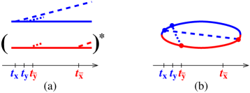
Figure 2: An example of an interference that contributes to the double splitting rate, drawn in the same style as fig. 1. A divergence of the form (7) arises from either the first three times approaching each other (depicted here) or the last three times approaching each other.

Refs. 2brem ; seq found that all the divergences (7) naively cancel each other in the sum over all interference contributions to the double splitting rate. But one must be careful, because finite contributions may still arise from the pole at $\Delta t=0$. As a simple mathematical example 2brem , the unregulated expression

$$\int_{0}^{\infty}\frac{d(\Delta t)}{\Delta t}-\int_{0}^{\infty}\frac{d(\Delta t)}{\Delta t}$$ (8)

naively looks to be zero, but if it were regularized as

$$\int_{0}^{\infty}\frac{d(\Delta t)}{\Delta t-i\epsilon}-\int_{0}^{\infty}\frac{d(\Delta t)}{\Delta t+i\epsilon}$$ (9)

then it would instead equal $i\pi$.

Ref. 2brem attempted to find $i\epsilon$ prescriptions for the poles, replacing each term (7) by

$$\operatorname{Re}\int_{0}d(\Delta t)\>\frac{i\Omega}{\Delta t\pm i\epsilon}$$ (10)

after arguing what the sign $\pm$ of the $i\epsilon$ prescription should be for each interference contribution to the double splitting rate. Unfortunately, this prescription turns out to miss some additional contributions from $\Delta t=0$. After discussing a relatively simple diagnostic test, we will explain (in section II.2) what went wrong with the substitution (10).

For reasons we will discuss later, attempting to fix up the $i\epsilon$ method for evaluating the pole contributions in double splitting seems complicated and fraught with subtlety. Fortunately, there is a cleaner, surer way to deal with the UV regularization of individual diagrams: We will show how to use dimensional regularization to compute the pole contributions from $\Delta t=0$. Dimensional regularization will turn the UV-divergent integral $\int_{0}d(\Delta t)/\Delta t$ in (7) into the UV-regularized integral $\int_{0}d(\Delta t)/(\Delta t)^{1-\epsilon/2}$. Reassuringly, we find that dimensional regularization passes our diagnostic.

The precise details of exactly how and why, for each diagram, the earlier work 2brem chose the sign of $\pm i\epsilon$ in the denominator of (10) will not be very important to the current discussion. However, for interested readers, we give a very brief review in appendix B.

I.2 Outline and Referencing

In the next section, we present a diagnostic that any consistent UV regularization scheme should satisfy. We then discuss what a successful $i\epsilon$ prescription would have to do to pass that test and show how the simple prescription (10) fails. We will characterize the type of contributions that (10) misses (which we call “$1/\pi^{2}$” pole pieces). In section III, we turn to dimensional regularization by warming up with the case of the single splitting rate (1). Sections IV and V then apply dimensional regularization to overlapping double splitting, treating, respectively, what we call the “crossed” interference diagrams of fig. 3 and the “sequential” diagrams of fig. 4. Section VI verifies that dimensional regularization passes the diagnostic test of section II. Finally, we present a summary of results in section VII. Various matters along the way are left for appendices.

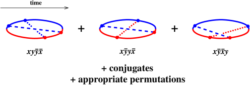
Figure 3: Interference contributions contributing to double splitting, showing the subset referred to as “crossed” diagrams in ref. 2brem . For QED double bremsstrahlung, the “appropriate permutations” are simply $x\leftrightarrow y$. For $g\to ggg$ in QCD, they are instead all permutations of $x$, $y$, and $z\equiv 1{-}x{-}y$.

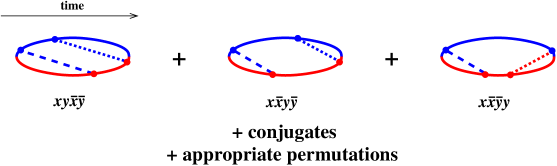
Figure 4: As fig. 3 except for the “sequential” diagrams of ref. seq .

In this paper, we will occasionally (in footnotes and appendices) use the author acronyms AI and ACI as shorthand for Arnold and Iqbal 2brem and Arnold, Chang and Iqbal seq so that, for example, we may write “ACI (5.2)” to refer to eq. (5.2) of ref. seq .

II A diagnostic

II.1 The QED independent emission test

Consider the case of double bremsstrahlung in QED, such as shown in fig. 5. In particular, consider the soft limit where the momentum fractions $x$ and $y$ carried by the two photons are small: $x,y\ll 1$. In that case, the backreaction on the initial high-energy electron is negligible, and so we might expect that the $x$ and $y$ emission are independent from each other:

$$\frac{dI}{dx\,dy}\simeq\frac{dI}{dx}\times\frac{dI}{dy},$$ (11)

where $dI/dx\,dy$ is the differential probability for double bremsstrahlung and $dI/dx$ is the differential probability for single bremsstrahlung. We will refer to (11), and similar formulas later for emission rates, as the independent emission model.

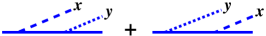
Figure 5: Amplitude for double bremsstrahlung in QED.

Now consider an idealized Monte Carlo (IMC) description of shower development, based on the rates for single splitting (such as single bremsstrahlung and single pair production). In ref. seq , it is explained that the important quantity for characterizing corrections to such a Monte Carlo due to overlapping formation times is the difference of actual double splitting rates from what such a Monte Carlo would predict for two consecutive splittings:

$$\Delta\,\frac{d\Gamma}{dx\,dy}\equiv\frac{d\Gamma}{dx\,dy}-\left[\frac{d\Gamma}{dx\,dy}\right]_{\rm IMC}.$$ (12)

However, the independent emission approximation described above already assumed that there were no effects from overlapping formation times, and so

$$\Delta\,\frac{d\Gamma}{dx\,dy}=0$$ (13)

in the independent emission approximation for $d\Gamma/dx\,dy$. This seems trivial. Nonetheless, we will obtain below an interesting test by reorganizing the individual terms that contribute to (13).

We have chosen QED rather than QCD bremsstrahlung for our test because the independent emission approximation is not the same thing as the Monte Carlo approximation to double bremsstrahlung in QCD. QCD Monte Carlo based on single splitting rates allows for the second bremsstrahlung to be independently emitted from either daughter of the first bremsstrahlung process, as shown in fig 6. That means that the Monte Carlo probability of $y$ emission is different depending on whether the $y$ emission happens before or after the $x$ emission. For QCD, Monte Carlo is therefore inconsistent with the independent emission model of (11), since in (11) the two emissions do not affect each other in any way.

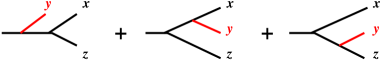
Figure 6: Idealized Monte Carlo (IMC) picture of two successive splittings in QCD.

To turn (13) into a test, split $d\Gamma/dx\,dy$ for double bremsstrahlung into a sum over the different possible time orderings of the emissions, shown in figs. 3 and 4. Then, in the independent emission approximation,

$$2\operatorname{Re}(xy\bar{y}\bar{x}+x\bar{y}y\bar{x}+x\bar{y}\bar{x}y+xy\bar{x}\bar{y}+x\bar{x}y\bar{y}+x\bar{x}\bar{y}y)+(x\leftrightarrow y)-{\rm IMC}=0.$$ (14)

Following refs. 2brem ; seq , the notation $xy\bar{y}\bar{x}$ indicates that the emissions in the corresponding diagram of fig. 3 happen in the time order of (i) $x$ emission in the amplitude, followed by (ii) $y$ emission in the amplitude, followed by (iii) $y$ emission in the conjugate amplitude, and finally (iv) $x$ emission in the conjugate amplitude.

There are two ways to make use of (14). One is to apply it to the full calculation (as opposed to the independent emission approximation) of the different double bremsstrahlung interference diagrams in QED, expand the results in small $x$ and $y$, and then check whether the equality (14) holds to leading order in that expansion.

The other use is to directly investigate how (14) works in the independent emission model itself, using one’s favorite UV regularization of single bremsstrahlung rates. We’ll now do just that for the case of $i\epsilon$ prescriptions.

II.2 Application to $i\epsilon$ prescriptions

Consider use of an $i\epsilon$ prescription to UV-regulate the single splitting rate of (1):

$$\frac{d\Gamma}{dx}=-\frac{\alpha P(x)}{\pi}\operatorname{Re}\int_{0}^{\infty}d(\Delta t_{x})\>\Omega^{2}\csc^{2}\bigl{(}\Omega(\Delta t_{x}-i\epsilon)\bigr{)}.$$ (15)

Appendix C shows that the test (14) is indeed satisfied (as it must be) if we use (15) in the independent emission model. Here we want to focus on the UV contributions to that test, which we have summarized in the second column of Table 1. That column shows the small $\Delta t$ limit of the $d(\Delta t)$ integrands for each diagram, corresponding to the pole pieces in (7). In this table, we have further assumed $y\ll x$ just to make the formulas as simple (and so easy to compare) as possible, and we have also introduced the short-hand notation

$$\Delta t_{\pm}\equiv\Delta t\pm i\epsilon.$$ (16)

	independent emission	$i\epsilon$ method
	approximation	of ref. 2brem
$2\operatorname{Re}(yx\bar{x}\bar{y})$	0	same
$2\operatorname{Re}(y\bar{x}x\bar{y})$	0	same
$2\operatorname{Re}(xy\bar{y}\bar{x})$	$\frac{1}{2}\operatorname{Re}\bigl{(}\frac{i\Omega_{x}}{\Delta t_{-}}\bigr{)}$	same
$2\operatorname{Re}(x\bar{y}y\bar{x})$	$\frac{1}{2}\operatorname{Re}\bigl{(}\frac{i\Omega_{x}\Delta t_{-}}{(\Delta t_{+})^{2}}\bigr{)}$	$\frac{1}{2}\operatorname{Re}\bigl{(}\frac{i\Omega_{x}}{\Delta t_{+}}\bigr{)}$
$2\operatorname{Re}(x\bar{y}\bar{x}y)$	$-\frac{1}{2}\operatorname{Re}\bigl{(}\frac{i\Omega_{x}}{\Delta t_{+}}\bigr{)}$	same
$2\operatorname{Re}(\bar{y}xy\bar{x})$	$-\frac{1}{2}\operatorname{Re}\bigl{(}\frac{i\Omega_{x}}{\Delta t_{+}}\bigr{)}$	same
$2\operatorname{Re}(xy\bar{x}\bar{y})$	$-\frac{1}{2}\operatorname{Re}\bigl{(}\frac{i\Omega_{x}}{\Delta t_{-}}\bigr{)}$	same
$2\operatorname{Re}(yx\bar{y}\bar{x})$	$-\frac{1}{2}\operatorname{Re}\bigl{(}\frac{i\Omega_{x}}{\Delta t_{-}}\bigr{)}$	same
$2\operatorname{Re}(x\bar{x}y\bar{y}+x\bar{x}\bar{y}y)+(x\leftrightarrow y)-{\rm IMC}$	$\Delta t\operatorname{Re}(i\Omega_{x})\operatorname{Re}\bigl{(}\frac{1}{(\Delta t_{-})^{2}}\bigr{)}$	$\operatorname{Re}(i\Omega_{x})\operatorname{Re}\bigl{(}\frac{1}{\Delta t_{-}}\bigr{)}$

Table 1: The UV ($\Delta t\to 0$) behavior of individual contributions to the test (14) for QED double bremsstrahlung in the limit $y\ll x\ll 1$. Purely-vacuum divergences ($\hat{q}=0$) have already been subtracted and are not shown. (See appendix C for additional clarification on what is included here.) Above, $\Delta t_{\pm}\equiv\Delta t\pm i\epsilon$. Each entry is to be integrated over (small) $\Delta t$ as in (7) and multiplied by $4\alpha_{\scriptscriptstyle\rm EM}^{2}/\pi^{2}xy$, where $\alpha_{\scriptscriptstyle\rm EM}$ is the fine structure constant. The small-$x$ complex frequency $\Omega_{x}$ above is defined by $\Omega_{x}^{\scriptscriptstyle\rm QED}\equiv\sqrt{-ix\hat{q}/2E}$. Following ref. 2brem , $\Delta t$ (no subscript) above is defined as the time separation between the middle two emissions for all but the last entry: e.g. $\Delta t\equiv t_{\bar{\rm y}}-t_{\rm y}$ for $xy\bar{y}\bar{x}$ and $\Delta t\equiv t_{\bar{\rm x}}-t_{\bar{\rm y}}$ for $x\bar{y}\bar{x}y$. All other times have been integrated over. (For the identification of $\Delta t$ in the last entry, see section IIA of ref. seq or appendix C.4 here.)

One may now see the problem with the earlier proposal (10) of ref. 2brem for how to regulate the $1/\Delta t$ poles in double bremsstrahlung calculations using the $i\epsilon$ prescription. It is true that, if you ignore $\epsilon$ prescriptions, then all of the small-$\Delta t$ divergences in Table 1 take the form $1/\Delta t$. But this does not mean that putting in $i\epsilon$’s gives $1/(\Delta t\pm i\epsilon)$. For example, the $2\operatorname{Re}(x\bar{y}y\bar{x})$ entry of the table reads

$$2\operatorname{Re}\left[\frac{d\Gamma}{dx\,dy}\right]_{x\bar{y}y\bar{x}}\simeq\frac{4\alpha_{\scriptscriptstyle\rm EM}^{2}}{\pi^{2}xy}\int_{0}d(\Delta t)\>\frac{1}{2}\operatorname{Re}\Bigl{(}\frac{i\Omega_{x}(\Delta t-i\epsilon)}{(\Delta t+i\epsilon)^{2}}\Bigr{)}.$$ (17)

The problem with the earlier analysis of ref. 2brem is that it correctly identified the $i\epsilon$ prescription in denominators, but failed to realize that $1/\Delta t=(\Delta t)/(\Delta t)^{2}$ could also have different and important $i\epsilon$ dependence in a numerator. The prescription proposed by ref. 2brem is shown in the last column of table 1 and can be obtained from the second column by replacing the full $\Delta t$ dependence by just $1/\Delta t$, with the $i\epsilon$ dependence taken from the denominator in the second column. So, for instance, the $2\operatorname{Re}(x\bar{y}y\bar{x})$ contribution (17) is replaced by

$$2\operatorname{Re}\left[\frac{d\Gamma}{dx\,dy}\right]^{\rm naive}_{x\bar{y}y\bar{x}}\simeq\frac{4\alpha_{\scriptscriptstyle\rm EM}^{2}}{\pi^{2}xy}\int_{0}d(\Delta t)\>\frac{1}{2}\operatorname{Re}\Bigl{(}\frac{i\Omega_{x}}{\Delta t+i\epsilon}\Bigr{)}.$$ (18)

The difference between the prescriptions (17) and (18) gives an integral that is dominated by $\Delta t\sim\epsilon$ and so is a purely “pole” contribution that can be evaluated without needing to know how the integrand behaves for large $t$:

$$2\operatorname{Re}\biggl{(}\left[\frac{d\Gamma}{dx\,dy}\right]_{x\bar{y}y\bar{x}}-{} \left[\frac{d\Gamma}{dx\,dy}\right]^{\rm naive}_{x\bar{y}y\bar{x}}\biggr{)}$$

$$=\frac{2\alpha_{\scriptscriptstyle\rm EM}^{2}}{\pi^{2}xy}\operatorname{Re}\left\{i\Omega_{x}\int_{0}^{\infty}d(\Delta t)\left[\frac{(\Delta t-i\epsilon)}{(\Delta t+i\epsilon)^{2}}-\frac{1}{(\Delta t+i\epsilon)}\right]\right\}$$

$$=\frac{4\alpha_{\scriptscriptstyle\rm EM}^{2}}{\pi^{2}xy}\,\operatorname{Re}(-i\Omega_{x}).$$ (19)

The one other difference in Table 1 can be evaluated similarly. For the $y\ll x\ll 1$ limit of the QED independent emission approximation, the total difference (summing all contributions) between the correct $i\epsilon$ prescription and the naive prescription of (10) is

$$\frac{d\Gamma}{dx\,dy}-\left[\frac{d\Gamma}{dx\,dy}\right]^{\rm naive}\simeq\frac{4\alpha_{\scriptscriptstyle\rm EM}^{2}}{\pi^{2}xy}\,2\operatorname{Re}(-i\Omega_{x}).$$ (20)

This is non-zero. Because the independent emission calculation must (and does) satisfy the test (14), we see that the naive prescription of ref. 2brem does not.

Rather than only check this failure of the naive prescription in the context of the independent emission calculation, we have also done a full QED calculation (not making any assumptions about the size of $x$ and $y$) of the LPM effect in double bremsstrahlung, along lines similar to the QCD calculation in refs. 2brem ; seq . We have verified that the $y\ll x\ll 1$ limit of those full results reproduce the last column of table 1 if we use the naive $i\epsilon$ prescription of (10) following ref. 2brem . We have also verified that the diagnostic test (14) fails in this limit by exactly the amount (20). The details of the full QED calculation are not directly relevant to our current task, which is to find a clear, correct method for determining the UV contributions which works not just in the context of the QED independent emission approximation but generalizes to QCD and to any values of $x$ and $y$. So we will defer presenting the details of full QED results for double bremsstrahlung to future work.

Why do we not simply fix up the $i\epsilon$ prescription in the general case, to make it work correctly like in the second column of Table 1? Despite various attempts, we were unable to find a convincing generalization that worked outside of the limiting case of $y\ll x\ll 1$. We briefly discuss the issues we encountered in appendix E. Here, we will instead turn to dimensional regularization for the general case.

II.3 $1/\pi$ vs. $1/\pi^{2}$ pole terms

Before moving on, it is interesting to note a qualitative difference between what the naive $i\epsilon$ prescription does account for and what it does not. As an example, consider the naive prescription small-$\Delta t$ behavior (18). Use the identity

$$\frac{1}{\Delta t\mp i\epsilon}=\operatorname{P.P.}\frac{1}{\Delta t}\pm i\pi\,\delta(\Delta t),$$ (21)

where “$\operatorname{P.P.}$” indicates the principal part prescription. The real-valued $1/\Delta t$ integration terms (the “principal part” terms above) will cancel among all the diagrams, as mentioned earlier, leaving a finite total result. The pole contributions (in the naive $i\epsilon$ prescription) are given by the $i\pi\,\delta(\Delta t)$ term above. Note that this term is associated with an extra factor of $\pi$. So, for instance, the corresponding pole piece of (18) is given by

$$2\operatorname{Re}\left[\frac{d\Gamma}{dx\,dy}\right]^{\rm naive~{}pole}_{x\bar{y}y\bar{x}}\simeq\frac{4\alpha_{\scriptscriptstyle\rm EM}^{2}}{\pi^{2}xy}\int_{0}d(\Delta t)\>\frac{1}{2}\operatorname{Re}(\Omega_{x})\,\pi\,\delta(\Delta t)=\frac{\alpha_{\scriptscriptstyle\rm EM}^{2}}{\pi xy}\,\operatorname{Re}(\Omega_{x})$$ (22)

(in which integrating over only half a $\delta$ function is understood to give $\frac{1}{2}$). Looking at the factors of $\pi$ in (22), the original, naive $i\epsilon$ prescription (10) gives all of what we will call the “$1/\pi$” terms for the pole contribution. The correct analysis of the problem, in contrast, introduces additional $1/\pi^{2}$ pole contributions such as (20).

We should also mention that if one analyzes all the entries this way, then the $1/\pi$ terms produced by the third column of table 1 add up to zero. This turns out to be an artifact of the $y\ll x\ll 1$ limit, and there is no such cancellation in the more general case.

III Single splitting with dimensional regularization

We now turn to dimensional regularization and will start with the single splitting formula (1). As reviewed in the introduction, dealing with the UV divergence for single splitting by other means is trivial, but it will provide a simple and useful warm-up example.

III.1 Straightforward method

Following Zakharov Zakharov , one way to view the source of the single splitting formula (1) is as an effective 2-dimensional non-Hermitian non-relativistic quantum mechanics problem for the three high-energy particles shown in fig. 1b. Using symmetries of the problem, the three-particle quantum mechanics problem can be reduced to a one-particle quantum mechanics problem. In this language, the basic formula corresponding to fig. 1 is

$$\frac{d\Gamma}{dx}=\frac{\alpha P(x)}{[x(1-x)E]^{2}}\operatorname{Re}\int_{0}^{\infty}d(\Delta t)\>{\bm{\nabla}}_{{\bm{B}}_{\bar{\rm x}}}\cdot{\bm{\nabla}}_{{\bm{B}}_{\rm x}}\langle{\bm{B}}_{\bar{\rm x}},\Delta t|{\bm{B}}_{\rm x},0\rangle\Bigr{|}_{{\bm{B}}_{\bar{\rm x}}={\bm{B}}_{\rm x}=0},$$ (23)

where ${\bm{B}}$ is a single, convenient combination of the transverse positions of the three particles. For a more complete discussion in the notation used here, see section II of ref. 2brem . In the multiple scattering ($\hat{q}$) approximation appropriate for high energy particles traversing thick media, the problem turns out to become a harmonic oscillator problem with complex frequency $\Omega$ and mass

$$M=x(1{-}x)E.$$ (24)

For constant $\Omega$ (appropriate to the case of a thick, homogeneous medium), the propagator of a 2-dimensional harmonic oscillator is

$$\langle{\bm{B}},\Delta t|{\bm{B}}^{\prime},0\rangle=\frac{M\Omega\csc(\Omega\,\Delta t)}{2\pi i}\,\exp\Bigl{(}\tfrac{i}{2}M\Omega\bigl{[}({\bm{B}}^{2}+{\bm{B}}^{\prime 2})\cot(\Omega\Delta t)-2{\bm{B}}\cdot{\bm{B}}^{\prime}\csc(\Omega\Delta t)\bigr{]}\Bigr{)}.$$ (25)

Using this in (23) reproduces the earlier formula (1).

To implement dimensional regularization, we simply generalize the $d{=}2$ analysis for two transverse dimensions to an arbitrary number $d$ of transverse dimensions. (Note that we are defining $d$ to be the number of transverse spatial dimensions, not the total number of space-time dimensions, and so the real world is $d=2$ in this paper, not $d=4$.) The propagator for a $d$-dimensional Harmonic oscillator is

$$\langle{\bm{B}},\Delta t|{\bm{B}}^{\prime},0\rangle=\left(\frac{M\Omega\csc(\Omega\,\Delta t)}{2\pi i}\right)^{d/2}\exp\Bigl{(}\tfrac{i}{2}M\Omega\bigl{[}({\bm{B}}^{2}+{\bm{B}}^{\prime 2})\cot(\Omega\Delta t)-2{\bm{B}}\cdot{\bm{B}}^{\prime}\csc(\Omega\Delta t)\bigr{]}\Bigr{)}.$$ (26)

The corresponding integral in (23) is then

$$\int_{0}^{\infty}d(\Delta t)\>{\bm{\nabla}}_{{\bm{B}}_{\bar{\rm x}}}\cdot{\bm{\nabla}}_{{\bm{B}}_{\rm x}} \langle{\bm{B}}_{\bar{\rm x}},\Delta t|{\bm{B}}_{\rm x},0\rangle\Bigr{|}_{{\bm{B}}_{\bar{\rm x}}={\bm{B}}_{\rm x}=0}$$

$$=-\int_{0}^{\infty}d(\Delta t)\>\left(\frac{M\Omega\csc(\Omega\,\Delta t)}{2\pi i}\right)^{d/2}idM\Omega\csc(\Omega\,\Delta t)$$ (27)

(using ${\bm{\nabla}}_{\bm{B}}\cdot{\bm{B}}=d$). Changing integration variable to $\tau\equiv i\Omega\,\Delta t$, this becomes

$$=-idM\left(\frac{M\Omega}{2\pi}\right)^{d/2}\int_{0}^{\infty}\frac{d\tau}{\operatorname{sh}^{1+\frac{d}{2}}\tau}\,.$$ (28)

We’ve been seemingly cavalier here about the complex phase of the upper limit of integration—see appendix A for a more careful discussion.

The integral (28) converges for $-2<d<0$. The result for other $d$ is defined by analytic continuation, giving (see appendix A)

$$\int_{0}^{\infty}d(\Delta t)\>{\bm{\nabla}}_{{\bm{B}}_{\bar{\rm x}}}\cdot{\bm{\nabla}}_{{\bm{B}}_{\rm x}}\langle{\bm{B}}_{\bar{\rm x}},\Delta t|{\bm{B}}_{\rm x},0\rangle\Bigr{|}_{{\bm{B}}_{\bar{\rm x}}={\bm{B}}_{\rm x}=0}=-\frac{idM}{2}\left(\frac{M\Omega}{2\pi}\right)^{d/2}\operatorname{B}(\tfrac{1}{2}{+}\tfrac{d}{4},-\tfrac{d}{4}),$$ (29)

where

$$\operatorname{B}(x,y)=\frac{\Gamma(x)\,\Gamma(y)}{\Gamma(x+y)}$$ (30)

is the Euler beta function.

We can now take the $d\to 2$ limit, giving

$$\int_{0}^{\infty}d(\Delta t)\>{\bm{\nabla}}_{{\bm{B}}_{\bar{\rm x}}}\cdot{\bm{\nabla}}_{{\bm{B}}_{\rm x}}\langle{\bm{B}}_{\bar{\rm x}},\Delta t|{\bm{B}}_{\rm x},0\rangle\Bigr{|}_{{\bm{B}}_{\bar{\rm x}}={\bm{B}}_{\rm x}=0}\to\frac{iM^{2}\Omega}{\pi}$$ (31)

Because this regularized result for the integral is finite for $d{=}2$, we do not have to worry about the generalization of the prefactor $\alpha P(x)/[x(1{-}x)E]^{2}$ in the $d\Gamma/dx$ formula (23) to general dimension: we can just use the known $d{=}2$ version. Combining (23), (24) and (31) correctly reproduces the usual result (4) for single splitting.

III.2 Alternative derivation

Before we launch into the complexities of the double bremsstrahlung calculation, we can introduce another formula that we will need by repeating the previous calculation in a slightly more roundabout manner: We will do the $\Delta t$ integral in (23) before taking the ${\bm{B}}_{\bar{\rm x}}$ derivative and so also before setting ${\bm{B}}_{\bar{\rm x}}$ to zero. The integral we need has the form

$$\int_{0}^{\infty}d(\Delta t)\>{\bm{\nabla}}_{{\bm{B}}^{\prime}}\langle{\bm{B}},\Delta t|{\bm{B}}^{\prime},0\rangle\Bigr{|}_{{\bm{B}}^{\prime}=0}.$$ (32)

Using the $d$-dimensional propagator (26), this becomes

$$=-iM{\bm{B}}\left(\frac{M\Omega}{2\pi}\right)^{d/2}\int_{0}^{\infty}\frac{d\tau}{\operatorname{sh}^{1+\frac{d}{2}}\tau}\,e^{-\frac{1}{2}M\Omega B^{2}\operatorname{cth}\tau},$$ (33)

with $\tau\equiv i\Omega\,\Delta t$ as before. The integral converges for $d>-2$ when ${\bm{B}}\not=0$. Using

$$\int_{0}^{\infty}d\tau\>\frac{e^{-z\operatorname{cth}\tau}}{\operatorname{sh}^{\frac{d}{2}+1}\tau}=\frac{\Gamma(\frac{1}{2}+\frac{d}{4})}{\sqrt{\pi}}\,\left(\frac{2}{z}\right)^{d/4}\,K_{d/4}(z)$$ (34)

(see appendix A), we obtain

$$\int_{0}^{\infty}d(\Delta t)\>{\bm{\nabla}}_{{\bm{B}}^{\prime}}\langle{\bm{B}},\Delta t|{\bm{B}}^{\prime},0\rangle\Bigr{|}_{{\bm{B}}^{\prime}=0}=-\frac{iM{\bm{B}}}{\pi^{(d+1)/2}}\left(\frac{M\Omega}{B^{2}}\right)^{d/4}\Gamma(\tfrac{1}{2}{+}\tfrac{d}{4})\,K_{d/4}(\tfrac{1}{2}M\Omega B^{2}).$$ (35)

This is a formula we will need later for double splitting, where it will be convenient to rewrite it equivalently as

$$\int_{-\infty}^{t}dt^{\prime}\>{\bm{\nabla}}_{{\bm{B}}^{\prime}}\langle{\bm{B}},t|{\bm{B}}^{\prime},t^{\prime}\rangle\Bigr{|}_{{\bm{B}}^{\prime}=0}=-\frac{iM{\bm{B}}}{\pi^{(d+1)/2}}\left(\frac{M\Omega}{B^{2}}\right)^{d/4}\Gamma(\tfrac{1}{2}{+}\tfrac{d}{4})\,K_{d/4}(\tfrac{1}{2}M\Omega B^{2}).$$ (36)

Let’s finish up the single splitting calculation by showing that we can use these formulas to get the same answer as before. We need to take the gradient ${\bm{\nabla}}_{\bm{B}}$ of (35) and set ${\bm{B}}$ to zero. The last step raises a subtlety which happily will not arise in the double splitting calculation later: the original integral (33) has convergence problems for ${\bm{B}}{=}0$ unless $d<0$. Eventually we want to focus on $d\to 2$, but we should be cautious about whether we analytically continue to that limit before or after setting ${\bm{B}}$ to zero. To see that there is an issue, use the generic expansion of the Bessel function for small arguments:

$$K_{\nu}(z)=\tfrac{1}{2}\,\Gamma(\nu)\,(\tfrac{z}{2})^{-\nu}\bigl{[}1+O(z^{2})\bigr{]}+\tfrac{1}{2}\,\Gamma(-\nu)\,(\tfrac{z}{2})^{\nu}\bigl{[}1+O(z^{2})\bigr{]}.$$ (37)

Which term dominates depends on the sign of $\nu$ and so, in our case, on the sign of $d$. Keeping both of the potentially leading terms above, the small ${\bm{B}}$ behavior of (35) is

$$\int_{0}^{\infty}d(\Delta t)\>{\bm{\nabla}}_{{\bm{B}}^{\prime}}\langle{\bm{B}},\Delta t|{\bm{B}}^{\prime},0\rangle\Bigr{|}_{{\bm{B}}^{\prime}=0}\\ \simeq-\frac{iM{\bm{B}}}{2}\left[\left(\frac{2}{\pi B^{2}}\right)^{d/2}\frac{\Gamma(\tfrac{1}{2}{+}\tfrac{d}{4})\,\Gamma(\tfrac{d}{4})}{\pi^{1/2}}+\left(\frac{M\Omega}{2\pi}\right)^{d/2}\operatorname{B}(\tfrac{1}{2}{+}\tfrac{d}{4},-\tfrac{d}{4})\right].$$ (38)

Now dot ${\bm{\nabla}}_{\bm{B}}$ into the above expression and then set ${\bm{B}}$ to zero. The second term gives exactly our earlier answer (29), which leads to the correct result (31) when we analytically continue to $d=2$. The first term gives a (UV) singularity unless $d\leq 0$. Since the point of dimensional regularization was to regulate the UV, we learn that in this application to single splitting we need to keep the dimension as $d<0$ until after we take ${\bm{B}}$ to zero.

IV Crossed diagrams with dimensional regularization

We now turn to double bremsstrahlung, focusing on $g\to ggg$ and starting with the crossed diagrams of fig. 3, which were evaluated for $d{=}2$ (other than the missing $1/\pi^{2}$ pole terms) in ref. 2brem . As in ref. 2brem , we will start with the $xy\bar{y}\bar{x}$ diagram, to which the others can be related.

IV.1 First equations

Our starting point here will be the $d{=}2$ expression

$$\left[\frac{dI}{dx\,dy}\right]_{xy\bar{y}\bar{x}}= \frac{C_{\rm A}^{2}\alpha_{\rm s}^{2}}{8E^{4}}\,\frac{(\alpha\delta^{\bar{n}n}\delta^{\bar{m}m}{+}\beta\delta^{\bar{n}\bar{m}}\delta^{nm}{+}\gamma\delta^{\bar{n}m}\delta^{n\bar{m}})}{|\hat{x}_{1}+\hat{x}_{4}||\hat{x}_{3}+\hat{x}_{4}|}\int_{t_{\rm x}<t_{\rm y}<t_{\bar{\rm y}}<t_{\bar{\rm x}}}$$

$$\int_{{\bm{B}}^{\bar{\rm y}},{\bm{B}}^{\rm y}}\nabla_{{\bm{B}}^{\bar{\rm x}}}^{\bar{n}}\langle{\bm{B}}^{\bar{\rm x}},t_{\bar{\rm x}}|{\bm{B}}^{\bar{\rm y}},t_{\bar{\rm y}}\rangle\Bigr{|}_{{\bm{B}}^{\bar{\rm x}}=0}$$

$$\qquad\times\nabla_{{\bm{C}}_{12}^{\bar{\rm y}}}^{\bar{m}}\nabla_{{\bm{C}}_{23}^{\rm y}}^{n}\langle{\bm{C}}_{34}^{\bar{\rm y}},{\bm{C}}_{12}^{\bar{\rm y}},t_{\bar{\rm y}}|{\bm{C}}_{41}^{\rm y},{\bm{C}}_{23}^{\rm y},t_{\rm y}\rangle\Bigr{|}_{{\bm{C}}_{12}^{\bar{\rm y}}=0={\bm{C}}_{23}^{\rm y};~{}{\bm{C}}_{34}^{\bar{\rm y}}={\bm{B}}^{\bar{\rm y}};~{}{\bm{C}}_{41}^{\rm y}={\bm{B}}^{\rm y}}$$

$$\qquad\times\nabla_{{\bm{B}}^{\rm x}}^{m}\langle{\bm{B}}^{\rm y},t_{\rm y}|{\bm{B}}^{\rm x},t_{\rm x}\rangle\Bigr{|}_{{\bm{B}}^{\rm x}=0}$$ (39)

developed for $xy\bar{y}\bar{x}$ in section IV of ref. 2brem . $\langle{\bm{B}}^{\rm y},t_{\rm y}|{\bm{B}}^{\rm x},t_{\rm x}\rangle$ and $\langle{\bm{C}}_{34}^{\bar{\rm y}},{\bm{C}}_{12}^{\bar{\rm y}},t_{\bar{\rm y}}|{\bm{C}}_{41}^{\rm y},{\bm{C}}_{23}^{\rm y},t_{\rm y}\rangle$ and $\langle{\bm{B}}^{\bar{\rm x}},t_{\bar{\rm x}}|{\bm{B}}^{\bar{\rm y}},t_{\bar{\rm y}}\rangle$ represent, respectively, the (i) 3-particle evolution of the system in the initial time interval $t_{\rm x}<t<t_{\rm y}$ of the figure, (ii) 4-particle evolution in the intermediate interval $t_{\rm y}<t<t_{\bar{\rm y}}$, and (iii) 3-particle evolution of the system in the final interval $t_{\bar{\rm y}}<t<t_{\bar{\rm x}}$. Because of the symmetries of the problem, these have been reduced to effective (i) 1-particle, (ii) 2-particle, and (iii) 1-particle problems in non-Hermitian $d{=}2$ quantum mechanics. Each vertex in the diagram is associated with one of the gradients above. The dimensionless functions $\alpha(x,y)$, $\beta(x,y)$, and $\gamma(x,y)$ contain normalization factors and combinations of spin-dependent DGLAP splitting functions associated with those vertices. The variables $\hat{x}_{i}$ refer to the momentum fractions associated with the four particles involved in the 4-particle evolution in this diagram, which are

$$(\hat{x}_{1},\hat{x}_{2},\hat{x}_{3},\hat{x}_{4})=(-1,y,1{-}x{-}y,x).$$ (40)

The overall factors of $|\hat{x}_{1}+\hat{x}_{4}|^{-1}$ and $|\hat{x}_{3}+\hat{x}_{4}|^{-1}$ are additional normalization factors associated with the vertices at the intermediate times $t_{\rm y}$ and $t_{\bar{\rm y}}$ given our choice of normalization of the transverse position variables and of corresponding states such as $|{\bm{C}}_{41},{\bm{C}}_{23}\rangle$ and $|{\bm{B}}\rangle$. The expression (39) also assumes the large $N_{\rm c}$ limit in order to simplify the color dynamics of the problem associated with the 4-particle propagation in the medium. However, we believe that the results for the pole contributions calculated in this paper do not depend on the assumption of large $N_{\rm c}$ because the 4-particle propagation in pole contributions is effectively vacuum propagation (as discussed earlier with regards to fig. 2).

The $d$-dimensional generalization of (39) is

$$\left[\frac{dI}{dx\,dy}\right]_{xy\bar{y}\bar{x}}= \frac{C_{\rm A}^{2}\alpha_{\rm s}^{2}}{8E^{2d}}\,\frac{(\alpha\delta^{\bar{n}n}\delta^{\bar{m}m}{+}\beta\delta^{\bar{n}\bar{m}}\delta^{nm}{+}\gamma\delta^{\bar{n}m}\delta^{n\bar{m}})}{|\hat{x}_{1}+\hat{x}_{4}|^{d/2}|\hat{x}_{3}+\hat{x}_{4}|^{d/2}}\int_{t_{\rm x}<t_{\rm y}<t_{\bar{\rm y}}<t_{\bar{\rm x}}}$$

$$\int_{{\bm{B}}^{\bar{\rm y}},{\bm{B}}^{\rm y}}\nabla_{{\bm{B}}^{\bar{\rm x}}}^{\bar{n}}\langle{\bm{B}}^{\bar{\rm x}},t_{\bar{\rm x}}|{\bm{B}}^{\bar{\rm y}},t_{\bar{\rm y}}\rangle\Bigr{|}_{{\bm{B}}^{\bar{\rm x}}=0}$$

$$\qquad\times\nabla_{{\bm{C}}_{12}^{\bar{\rm y}}}^{\bar{m}}\nabla_{{\bm{C}}_{23}^{\rm y}}^{n}\langle{\bm{C}}_{34}^{\bar{\rm y}},{\bm{C}}_{12}^{\bar{\rm y}},t_{\bar{\rm y}}|{\bm{C}}_{41}^{\rm y},{\bm{C}}_{23}^{\rm y},t_{\rm y}\rangle\Bigr{|}_{{\bm{C}}_{12}^{\bar{\rm y}}=0={\bm{C}}_{23}^{\rm y};~{}{\bm{C}}_{34}^{\bar{\rm y}}={\bm{B}}^{\bar{\rm y}};~{}{\bm{C}}_{41}^{\rm y}={\bm{B}}^{\rm y}}$$

$$\qquad\times\nabla_{{\bm{B}}^{\rm x}}^{m}\langle{\bm{B}}^{\rm y},t_{\rm y}|{\bm{B}}^{\rm x},t_{\rm x}\rangle\Bigr{|}_{{\bm{B}}^{\rm x}=0}$$ (41)

There are no important changes to this formula other than the fact that transverse positions ${\bm{B}}$ and ${\bm{C}}$ are now $d$-dimensional, but we should comment on the other, mostly unimportant differences between (39) and (41):

• The functions $\alpha$, $\beta$, and $\gamma$ will be different in $d$ dimensions. For one thing, the number of “helicities” to be summed over depends on $d$. Except as noted below, we absorb all this dependence on $d$ into new $d$-dimensional versions of $\alpha$, $\beta$, and $\gamma$. However, similar to the discussion of $P(x)$ in section III.1, we will see when we take $d\to 2$ at the end of the day that we only need explicit formulas for the original $d{=}2$ versions given in ref. 2brem .

• One of the exceptions to absorbing all of the differences into the $d$-dimensional definitions of $(\alpha,\beta,\gamma)$: We have changed the overall $E^{-4}$ in (39) to $E^{-2d}$ in order to keep $\alpha$, $\beta$, and $\gamma$ dimensionless (and so make dimensional analysis of our formulas easier). This difference originates with the factors of $E$ associated with the vertices (see appendix A).

• We have also treated separately the generalization of the normalization factors $|x_{1}{+}x_{4}|^{-1}|x_{3}{+}x_{4}|^{-1}$ to $|x_{1}{+}x_{4}|^{-d/2}|x_{3}{+}x_{4}|^{-d/2}$ (see appendix A). The reason that we do not also absorb these differences is that, unlike $(\alpha,\beta,\gamma)$, these factors will not be the same for the three diagrams shown explicitly in fig. 3. Since we will later relate these diagrams to each other, we need to keep track of factors that change between them. These factors are nonetheless fairly uninteresting because $|x_{1}{+}x_{4}|^{-d/2}|x_{3}{+}x_{4}|^{-d/2}$ will simply cancel some related normalization factors when we later write more explicit formulas for the 4-particle propagator.

We now want to use (36) to integrate over the first time $t_{\rm x}$ in (41). The derivation of (36) relied on the $M$ associated with the 3-particle evolution being positive, and the associated $\Omega$ having phase $\sqrt{-i}$. All is well for now, but when we later relate the other crossed diagrams to $xy\bar{y}\bar{x}$, we will encounter situations where instead both $M$ is negative and $\Omega\propto\sqrt{+i}$. It’s therefore convenient to use an appropriate generalization of (36) to cover both situations:

$$\int_{-\infty}^{t}dt^{\prime}\>{\bm{\nabla}}_{{\bm{B}}^{\prime}}\langle{\bm{B}},t|{\bm{B}}^{\prime},t^{\prime}\rangle\Bigr{|}_{{\bm{B}}^{\prime}=0}=-\frac{iM{\bm{B}}}{\pi^{(d+1)/2}}\left(\frac{|M|\Omega}{B^{2}}\right)^{d/4}\Gamma(\tfrac{1}{2}{+}\tfrac{d}{4})\,K_{d/4}(\tfrac{1}{2}|M|\Omega B^{2})$$ (42a)

(see appendix A). The similar result for integration over the final time is

$$\int_{t^{\prime}}^{\infty}dt\>{\bm{\nabla}}_{{\bm{B}}}\langle{\bm{B}},t|{\bm{B}}^{\prime},t^{\prime}\rangle\Bigr{|}_{{\bm{B}}=0}=-\frac{iM{\bm{B}}^{\prime}}{\pi^{(d+1)/2}}\left(\frac{|M|\Omega}{B^{\prime 2}}\right)^{d/4}\Gamma(\tfrac{1}{2}{+}\tfrac{d}{4})\,K_{d/4}(\tfrac{1}{2}|M|\Omega B^{\prime 2}).$$ (42b)

Using these for the initial $t_{\rm x}$ and final $t_{\bar{\rm x}}$ time integrations in (41) gives

$$\left[\frac{d\Gamma}{dx\,dy}\right]_{xy\bar{y}\bar{x}}= -\frac{C_{\rm A}^{2}\alpha_{\rm s}^{2}M_{\rm i}M_{\rm f}}{8\pi^{d+1}E^{2d}}\frac{(\alpha\delta^{\bar{n}n}\delta^{\bar{m}m}{+}\beta\delta^{\bar{n}\bar{m}}\delta^{nm}{+}\gamma\delta^{\bar{n}m}\delta^{n\bar{m}})}{|\hat{x}_{1}+\hat{x}_{4}|^{d/2}|\hat{x}_{3}+\hat{x}_{4}|^{d/2}}\>\Gamma^{2}(\tfrac{1}{2}{+}\tfrac{d}{4})\,$$

$$\times\int_{0}^{\infty}d(\Delta t)\int_{{\bm{B}}^{\bar{\rm y}},{\bm{B}}^{\rm y}}B^{{\bar{\rm y}}}_{\bar{n}}\left(\frac{|M_{\rm f}|\Omega_{\rm f}}{(B^{\bar{\rm y}})^{2}}\right)^{d/4}K_{d/4}\bigl{(}\tfrac{1}{2}|M_{\rm f}|\Omega_{\rm f}(B^{\bar{\rm y}})^{2}\bigr{)}$$

$$\qquad\times B^{{\rm y}}_{m}\left(\frac{|M_{\rm i}|\Omega_{\rm i}}{(B^{\rm y})^{2}}\right)^{d/4}K_{d/4}\bigl{(}\tfrac{1}{2}|M_{\rm i}|\Omega_{\rm i}(B^{\rm y})^{2}\bigr{)}$$

$$\qquad\times\nabla_{{\bm{C}}_{12}^{\bar{\rm y}}}^{\bar{m}}\nabla_{{\bm{C}}_{23}^{\rm y}}^{n}\langle{\bm{C}}_{34}^{\bar{\rm y}},{\bm{C}}_{12}^{\bar{\rm y}},\Delta t|{\bm{C}}_{41}^{\rm y},{\bm{C}}_{23}^{\rm y},0\rangle\Bigr{|}_{{\bm{C}}_{12}^{\bar{\rm y}}=0={\bm{C}}_{23}^{\rm y};~{}{\bm{C}}_{34}^{\bar{\rm y}}={\bm{B}}^{\bar{\rm y}};~{}{\bm{C}}_{41}^{\rm y}={\bm{B}}^{\rm y}},$$ (43)

where $(M_{\rm i},\Omega_{\rm i})$ are associated with the initial 3-particle evolution ($t_{\rm x}<t<t_{\rm y}$) and $(M_{\rm f},\Omega_{\rm f})$ with the final 3-particle evolution ($t_{\bar{\rm y}}<t<t_{\bar{\rm x}}$).

IV.2 4-particle propagator

For evaluation of the pole pieces (which are the pieces that require UV regularization), we only need the small $\Delta t$ limit of (43). In that limit, medium effects on the propagator $\langle{\bm{C}}_{34}^{\bar{\rm y}},{\bm{C}}_{12}^{\bar{\rm y}},\Delta t|{\bm{C}}_{41}^{\rm y},{\bm{C}}_{23}^{\rm y},0\rangle$ are small. We will therefore use the vacuum result for $\langle{\bm{C}}_{34}^{\bar{\rm y}},{\bm{C}}_{12}^{\bar{\rm y}},\Delta t|{\bm{C}}_{41}^{\rm y},{\bm{C}}_{23}^{\rm y},0\rangle$. (Readers who would prefer to see a derivation closer to ref. 2brem , where we first find full expressions for the propagator before taking the small $\Delta t$ limit to find the poles, may turn instead to Appendix F.)

As discussed in ref. 2brem , the effective 4-particle evolution in interference diagrams such as fig. 3 is given (in the high-energy limit) by a Lagrangian of the form

$$L=\tfrac{1}{2}\begin{pmatrix}\dot{\bm{C}}_{34}\\ \dot{\bm{C}}_{12}\end{pmatrix}^{\!\top}\!{\mathfrak{M}}\begin{pmatrix}\dot{\bm{C}}_{34}\\ \dot{\bm{C}}_{12}\end{pmatrix}-V({\bm{C}}_{34},{\bm{C}}_{12})$$ (44)

where

$${\bm{C}}_{ij}\equiv\frac{{\bm{b}}_{i}-{\bm{b}}_{j}}{x_{i}+x_{j}},$$ (45)

${\bm{b}}_{i}$ are the transverse positions of the individual particles, and

$${\mathfrak{M}}=\begin{pmatrix}x_{3}x_{4}(x_{3}+x_{4})&\\ &x_{1}x_{2}(x_{1}+x_{2})\end{pmatrix}E=\begin{pmatrix}x_{3}x_{4}&\\ &-x_{1}x_{2}\end{pmatrix}(x_{3}+x_{4})E.$$ (46)

The imaginary-valued potential $V$ implements medium effects which cause decoherence of interference over times $\Delta t$ of order the formation time. In vacuum, $V=0$. Were we to express the propagator associated with (44) solely in terms of the variables $({\bm{C}}_{34},{\bm{C}}_{12})$, it would then (in this limit) simply be

$$\langle{\bm{C}}_{34},{\bm{C}}_{12},\Delta t|{\bm{C}}^{\prime}_{34},{\bm{C}}^{\prime}_{12},0\rangle\simeq\\ (2\pi i\,\Delta t)^{-d}(\det{\mathfrak{M}})^{d/2}\exp\Biggl{[}\frac{i}{2\,\Delta t}\begin{pmatrix}{\bm{C}}_{34}{-}{\bm{C}}^{\prime}_{34}\\ {\bm{C}}_{12}{-}{\bm{C}}^{\prime}_{12}\end{pmatrix}^{\top}{\mathfrak{M}}\begin{pmatrix}{\bm{C}}_{34}{-}{\bm{C}}^{\prime}_{34}\\ {\bm{C}}_{12}{-}{\bm{C}}^{\prime}_{12}\end{pmatrix}\Biggr{]}.$$ (47)

Changing variables from $({\bm{C}}_{34},{\bm{C}}_{12})$ to $({\bm{C}}_{41},{\bm{C}}_{23})$ in just the ket $|{\bm{C}}^{\prime}_{34},{\bm{C}}^{\prime}_{12},0\rangle$ then gives the version of this propagator that we need:

$$\langle{\bm{C}}_{34},{\bm{C}}_{12},\Delta t| {\bm{C}}^{\prime}_{41},{\bm{C}}^{\prime}_{23},0\rangle\simeq(2\pi i\,\Delta t)^{-d}(\det{\mathfrak{M}})^{d/4}(\det{\mathfrak{M}}^{\prime})^{d/4}$$

$$\times\exp\Biggl{[}\frac{i}{2\,\Delta t}\begin{pmatrix}{\bm{C}}^{\prime}_{41}\\ {\bm{C}}^{\prime}_{23}\end{pmatrix}^{\top}\!{\mathfrak{M}}^{\prime}\begin{pmatrix}{\bm{C}}^{\prime}_{41}\\ {\bm{C}}^{\prime}_{23}\end{pmatrix}+\frac{i}{2\,\Delta t}\begin{pmatrix}{\bm{C}}_{34}\\ {\bm{C}}_{12}\end{pmatrix}^{\top}\!{\mathfrak{M}}\begin{pmatrix}{\bm{C}}_{34}\\ {\bm{C}}_{12}\end{pmatrix}$$

$$\qquad\quad+\frac{iE}{\Delta t}\begin{pmatrix}{\bm{C}}^{\prime}_{41}\\ {\bm{C}}^{\prime}_{23}\end{pmatrix}^{\top}\!\begin{pmatrix}x_{1}x_{3}x_{4}&x_{1}x_{2}x_{4}\\ x_{2}x_{3}x_{4}&x_{1}x_{2}x_{3}\end{pmatrix}\begin{pmatrix}{\bm{C}}_{34}\\ {\bm{C}}_{12}\end{pmatrix}\Biggr{]}$$ (48)

(see appendix A), where ${\mathfrak{M}}^{\prime}$ is the $1{\leftrightarrow}3$ permutation of ${\mathfrak{M}}$ (46),

$${\mathfrak{M}}^{\prime}=\begin{pmatrix}x_{1}x_{4}&\\ &-x_{2}x_{3}\end{pmatrix}(x_{1}+x_{4})E.$$ (49)

In order to keep notation as close as possible to ref. 2brem , it will be useful to rewrite the exponential in (48) as

$$\exp\Biggl{[}-\frac{1}{2}\begin{pmatrix}{\bm{C}}^{\prime}_{41}\\ {\bm{C}}^{\prime}_{23}\end{pmatrix}^{\top}\!\begin{pmatrix}{\cal X}_{\rm y}&Y_{\rm y}\\ Y_{\rm y}&Z_{\rm y}\end{pmatrix}\begin{pmatrix}{\bm{C}}^{\prime}_{41}\\ {\bm{C}}^{\prime}_{23}\end{pmatrix}-\frac{1}{2}\begin{pmatrix}{\bm{C}}_{34}\\ {\bm{C}}_{12}\end{pmatrix}^{\top}\!\begin{pmatrix}{\cal X}_{\bar{\rm y}}&Y_{\bar{\rm y}}\\ Y_{\bar{\rm y}}&Z_{\bar{\rm y}}\end{pmatrix}\begin{pmatrix}{\bm{C}}_{34}\\ {\bm{C}}_{12}\end{pmatrix}\\ +\begin{pmatrix}{\bm{C}}^{\prime}_{41}\\ {\bm{C}}^{\prime}_{23}\end{pmatrix}^{\top}\!\begin{pmatrix}X_{{\rm y}{\bar{\rm y}}}&Y_{{\rm y}{\bar{\rm y}}}\\ \overline{Y}_{{\rm y}{\bar{\rm y}}}&Z_{{\rm y}{\bar{\rm y}}}\end{pmatrix}\begin{pmatrix}{\bm{C}}_{34}\\ {\bm{C}}_{12}\end{pmatrix}\Biggr{]},$$ (50)

where

$$\begin{pmatrix}{\cal X}_{\rm y}&Y_{\rm y}\\ Y_{\rm y}&Z_{\rm y}\end{pmatrix} =-\frac{iE(x_{1}{+}x_{4})}{\Delta t}\begin{pmatrix}x_{1}x_{4}&0\\ 0&-x_{2}x_{3}\end{pmatrix}+O(\Delta t),$$ (51a)

$$\begin{pmatrix}{\cal X}_{\bar{\rm y}}&Y_{\bar{\rm y}}\\ Y_{\bar{\rm y}}&Z_{\bar{\rm y}}\end{pmatrix} =-\frac{iE(x_{3}{+}x_{4})}{\Delta t}\begin{pmatrix}x_{3}x_{4}&0\\ 0&-x_{1}x_{2}\end{pmatrix}+O(\Delta t),$$ (51b)

$$\begin{pmatrix}X_{{\rm y}{\bar{\rm y}}}&Y_{{\rm y}{\bar{\rm y}}}\\ \overline{Y}_{{\rm y}{\bar{\rm y}}}&Z_{{\rm y}{\bar{\rm y}}}\end{pmatrix} =\frac{iE}{\Delta t}\begin{pmatrix}x_{1}x_{3}x_{4}&x_{1}x_{2}x_{4}\\ x_{2}x_{3}x_{4}&x_{1}x_{2}x_{3}\end{pmatrix}+O(\Delta t).$$ (51c)

Here, the unspecified $+O(\Delta t)$ contributions represent the size of effects due to the medium. Using (48) and (50) in (43) then gives

$$\left[\frac{d\Gamma}{dx\,dy}\right]_{xy\bar{y}\bar{x}}\simeq -\frac{C_{\rm A}^{2}\alpha_{\rm s}^{2}M_{\rm i}M_{\rm f}}{2^{d+3}\pi^{2d+1}i^{d}E^{d}}\,\Gamma^{2}(\tfrac{1}{2}{+}\tfrac{d}{4})\,({-}\hat{x}_{1}\hat{x}_{2}\hat{x}_{3}\hat{x}_{4})^{d/2}(\alpha\delta^{\bar{n}n}\delta^{\bar{m}m}{+}\beta\delta^{\bar{n}\bar{m}}\delta^{nm}{+}\gamma\delta^{\bar{n}m}\delta^{n\bar{m}})$$

$$\times\int_{0}\frac{d(\Delta t)}{(\Delta t)^{d}}\int_{{\bm{B}}^{\bar{\rm y}},{\bm{B}}^{\rm y}}B^{{\bar{\rm y}}}_{\bar{n}}\left(\frac{|M_{\rm f}|\Omega_{\rm f}}{(B^{\bar{\rm y}})^{2}}\right)^{d/4}K_{d/4}\bigl{(}\tfrac{1}{2}|M_{\rm f}|\Omega_{\rm f}(B^{\bar{\rm y}})^{2}\bigr{)}$$

$$\times B^{{\rm y}}_{m}\left(\frac{|M_{\rm i}|\Omega_{\rm i}}{(B^{\rm y})^{2}}\right)^{d/4}K_{d/4}\bigl{(}\tfrac{1}{2}|M_{\rm i}|\Omega_{\rm i}(B^{\rm y})^{2}\bigr{)}$$

$$\times\bigl{[}(Y_{\rm y}{\bm{B}}^{\rm y}-\overline{Y}_{{\rm y}{\bar{\rm y}}}{\bm{B}}^{\bar{\rm y}})_{n}(Y_{\bar{\rm y}}{\bm{B}}^{\bar{\rm y}}-Y_{{\rm y}{\bar{\rm y}}}{\bm{B}}^{\rm y})_{\bar{m}}+Z_{{\rm y}{\bar{\rm y}}}\delta_{n\bar{m}}\bigr{]}$$

$$\times\exp\Bigl{[}-\tfrac{1}{2}{\cal X}_{\rm y}(B^{\rm y})^{2}-\tfrac{1}{2}{\cal X}_{\bar{\rm y}}(B^{\bar{\rm y}})^{2}+X_{{\rm y}{\bar{\rm y}}}{\bm{B}}^{\rm y}\cdot{\bm{B}}^{\bar{\rm y}}\Bigr{]}.$$ (52)

IV.3 Small ${\bm{B}}$ expansion

We could try to follow the $d{=}2$ analysis of ref. 2brem by next doing the two ${\bm{B}}$ integrations in (52). Unfortunately, the integrals are complicated. Fortunately, we can simply the calculation because we need general-$d$ expressions for only the pole pieces, corresponding to $\Delta t\to 0$. The exponential factors in (52) become highly oscillatory for $B\gg{\cal X}^{-1/2}\sim\sqrt{\Delta t/E}$ and so cause the integrals to be dominated by the scale $B\sim\sqrt{\Delta t/E}$ (where we are not showing the $x_{i}$ dependence). So, for the purpose of extracting the small $\Delta t$ behavior, we may expand the Bessel functions in (52) for small arguments, as in (37). For $-4<d<4$ (which includes both the physical point $d{=}2$ and the region $-2<d<0$ where all of our earlier integrals were convergent), the terms shown explicitly in (37) are the leading ones and give

$$\left(\frac{|M|\Omega}{B^{2}}\right)^{d/4}K_{d/4}(\tfrac{1}{2}|M|\Omega B^{2})\simeq\tfrac{1}{2}\,\Gamma(\tfrac{d}{4})\,\left(\frac{2}{B^{2}}\right)^{d/2}+\tfrac{1}{2}\,\Gamma(-\tfrac{d}{4})\,\left(\frac{|M|\Omega}{2}\right)^{d/2}.$$ (53)

We will see later that the integrals we have left to do converge for $d=2-\epsilon$ with $\epsilon$ small, and so we may as well take $d=2-\epsilon$ now. In that case, the first term in (53) dominates over the second. By itself, however, the first term is uninteresting because it does not depend on $\Omega$ and so does not depend on $\hat{q}$. If we use just the first term for both of the $(|M|\Omega/B^{2})^{d/4}K_{d/4}$ factors in (52), we will obtain a contribution that will be canceled when we subtract away the purely vacuum result. We should therefore focus on the next term:

$$\left(\frac{|M_{\rm f}|\Omega_{\rm f}}{(B^{\bar{\rm y}})^{2}}\right)^{d/4}K_{d/4}\bigl{(}\tfrac{1}{2}|M_{\rm f}|\Omega_{\rm f}(B^{\bar{\rm y}})^{2}\bigr{)}\times\left(\frac{|M_{\rm i}|\Omega_{\rm i}}{(B^{\rm y})^{2}}\right)^{d/4}K_{d/4}\bigl{(}\tfrac{1}{2}|M_{\rm i}|\Omega_{\rm i}(B^{\rm y})^{2}\bigr{)}\simeq\\ (\mbox{vacuum})+\tfrac{1}{4}\,\Gamma(\tfrac{d}{4})\,\Gamma(-\tfrac{d}{4})\,\left[\left(\frac{|M_{\rm i}|\Omega_{\rm i}}{(B^{\bar{\rm y}})^{2}}\right)^{d/2}+\left(\frac{|M_{\rm f}|\Omega_{\rm f}}{(B^{\rm y})^{2}}\right)^{d/2}\right]+(\mbox{sub-leading}).$$ (54)

The (non-vacuum) small $\Delta t$ limit of the integrand in (52) then gives

$$\left[\frac{d\Gamma}{dx\,dy}\right]_{xy\bar{y}\bar{x}}\simeq \frac{C_{\rm A}^{2}\alpha_{\rm s}^{2}M_{\rm i}M_{\rm f}}{2^{d+3}d\pi^{2d}i^{d}E^{d}}\,\frac{\Gamma^{2}(\tfrac{1}{2}{+}\tfrac{d}{4})}{\sin(\frac{\pi d}{4})}\,({-}\hat{x}_{1}\hat{x}_{2}\hat{x}_{3}\hat{x}_{4})^{d/2}(\alpha\delta^{\bar{n}n}\delta^{\bar{m}m}{+}\beta\delta^{\bar{n}\bar{m}}\delta^{nm}{+}\gamma\delta^{\bar{n}m}\delta^{n\bar{m}})$$

$$\times\int_{0}\frac{d(\Delta t)}{(\Delta t)^{d}}\>\int_{{\bm{B}}^{\bar{\rm y}},{\bm{B}}^{\rm y}}B^{{\bar{\rm y}}}_{\bar{n}}B^{{\rm y}}_{m}\left[\left(\frac{|M_{\rm i}|\Omega_{\rm i}}{(B^{\bar{\rm y}})^{2}}\right)^{d/2}+\left(\frac{|M_{\rm f}|\Omega_{\rm f}}{(B^{\rm y})^{2}}\right)^{d/2}\right]$$

$$\times\bigl{[}(Y_{\rm y}{\bm{B}}^{\rm y}-\overline{Y}_{{\rm y}{\bar{\rm y}}}{\bm{B}}^{\bar{\rm y}})_{n}(Y_{\bar{\rm y}}{\bm{B}}^{\bar{\rm y}}-Y_{{\rm y}{\bar{\rm y}}}{\bm{B}}^{\rm y})_{\bar{m}}+Z_{{\rm y}{\bar{\rm y}}}\delta_{n\bar{m}}\bigr{]}$$

$$\times\exp\Bigl{[}-\tfrac{1}{2}{\cal X}_{\rm y}(B^{\rm y})^{2}-\tfrac{1}{2}{\cal X}_{\bar{\rm y}}(B^{\bar{\rm y}})^{2}+X_{{\rm y}{\bar{\rm y}}}{\bm{B}}^{\rm y}\cdot{\bm{B}}^{\bar{\rm y}}\Bigr{]},$$ (55)

where we’ve used $\frac{1}{4}\,\Gamma(\tfrac{d}{4})\,\Gamma(-\tfrac{d}{4})=-\frac{\pi}{d}\csc(\frac{\pi d}{4})$ for the sake of compactness.

IV.4 Scaling

Before diving into the details of explicitly performing the ${\bm{B}}$ integrals in (55), it is worthwhile to see the general structure of the result using a simple scaling argument. We can quickly see the $\Delta t$ dependence by rescaling ${\bm{B}}=\hat{\bm{B}}\sqrt{\Delta t/E}$, where $\hat{\bm{B}}$ is dimensionless, and noting that $(X,Y,Z)\propto E/\Delta t$ in (51). This rescaling pulls out all of the $\Delta t$ (and $E$) dependence from the two $d^{d}B$ integrals, identifying the small $\Delta t$ behavior as

$$\left[\frac{d\Gamma}{dx\,dy}\right]_{xy\bar{y}\bar{x}}$$

$$\qquad\propto M_{\rm i}M_{\rm f}\left(\frac{|M_{\rm i}|\Omega_{\rm i}}{E^{3}}\right)^{d/2}\int\frac{d(\Delta t)}{(\Delta t)^{d/2}}\int_{\hat{\bm{B}}^{\bar{\rm y}},\hat{\bm{B}}^{\rm y}}(\mbox{dimensionless function of $\hat{\bm{B}}$s and $\{x_{j}\}$})$$

$$\qquad\qquad\qquad+[\mbox{similar for ${\rm i}\leftrightarrow{\rm f}$}]$$

$$\qquad=(\mbox{dimensionless function of $\{x_{j}\}$})\times E^{2}\left(\frac{\hat{q}}{E^{5}}\right)^{d/4}\int_{0}\frac{d(\Delta t)}{(\Delta t)^{d/2}}\,.$$ (56)

Note that this result has the right dimension to be $d\Gamma/dx\,dy$ and also gives the usual dependence $d\Gamma/dx\,dy\propto\sqrt{\hat{q}/E}$ on $\hat{q}$ and $E$ for $d=2$.

The UV behavior of the $\Delta t$ integral above is convergent and well-defined for $d=2-\epsilon$. On the infrared (IR) end of the integration region (large $\Delta t$), our small-$\Delta t$ expansion formulas are no longer valid. But the formulas above will be good enough to study the contribution we get, if any, from arbitrarily small $\Delta t$. Imagine taking the full expression for $d\Gamma/dx\,dy$ as an integral over $\Delta t$, without having made any small $\Delta t$ approximation. Then divide the integration region up into $\Delta t<a$ and $\Delta t>a$ for some $a$ chosen very small compared to the formation times in the problem:

$$\int_{0}^{\infty}d(\Delta t)\>\cdots=\int_{0}^{a}d(\Delta t)\>\cdots+\int_{a}^{\infty}d(\Delta t)\>\cdots.$$ (57)

The $\Delta t>a$ integration can be handled with the $d{=}2$ formulas of ref. 2brem : the difference between $d{=}2-\epsilon$ and $d{=}2$ in this region can be ignored as $\epsilon\to 0$. The UV contributions that required UV regularization appear only in the $\Delta t<a$ integration. In (56), that integration region gives

$$\int_{0}^{a}\frac{d(\Delta t)}{(\Delta t)^{(2-\epsilon)/2}}=\frac{2a^{\epsilon/2}}{\epsilon}=\frac{2}{\epsilon}+\ln a+O(\epsilon).$$ (58)

The $1/\epsilon$ and $\ln a$ terms will cancel between diagrams for the same reason that $1/\Delta t$ terms cancel between diagrams in ref. 2brem .

However, there can be finite $O(\epsilon^{0})$ contributions to diagrams that do not cancel. The UV piece of a diagram $D$ will have the generic form

$$f_{D}(\epsilon,\{x_{j}\})\int_{0}^{a}\frac{d(\Delta t)}{(\Delta t)^{(2-\epsilon)/2}}.$$ (59)

For the $xy\bar{y}\bar{x}$ diagram, for example, $f_{D}(\epsilon,\{x_{j}\})$ represents all the factors in (56) besides the $\Delta t$ integral. Now consider the sum of some set of diagrams,

$$\sum_{D}f_{D}(\epsilon,\{x_{j}\})\int_{0}^{a}\frac{d(\Delta t)}{(\Delta t)^{(2-\epsilon)/2}}\,,$$ (60)

for which the the $1/\Delta t$ pieces of the integrand cancel in $d{=}2$:

$$\sum_{D}f_{D}(0,\{x_{j}\})=0.$$ (61)

Using (58), we see that we can still get a non-vanishing result from (i) the $O(\epsilon)$ pieces of $f_{D}(\epsilon)$ multiplying (ii) the $2/\epsilon$ piece of (58):

$$\sum_{D}f_{D}(\epsilon,\{x_{j}\})\int_{0}^{a}\frac{d(\Delta t)}{(\Delta t)^{(2-\epsilon)/2}}=2\sum_{D}\frac{\partial f_{D}}{\partial\epsilon}(0,\{x_{j}\})+O(\epsilon).$$ (62)

This finite piece, which survives in the $a\to 0$ limit, represents the pole contribution that we are looking for: it is a contribution associated with $\Delta t=0$ in the limit $d\to 2$.

IV.5 Actually doing the ${\bm{B}}$ integrals

We now return to the unscaled ${\bm{B}}$’s, just to keep the discussion as close as possible to the $d{=}2$ analysis of ref. 2brem . Contracting the various transverse spatial indices $m$, $n$, $\bar{m}$, and $\bar{n}$ of (55) gives

$$\left[\frac{d\Gamma}{dx\,dy}\right]_{xy\bar{y}\bar{x}}\simeq \frac{C_{\rm A}^{2}\alpha_{\rm s}^{2}M_{\rm i}M_{\rm f}}{2^{d+3}d\pi^{2d}i^{d}E^{d}}\,\frac{\Gamma^{2}(\tfrac{1}{2}{+}\tfrac{d}{4})}{\sin(\frac{\pi d}{4})}\,\bigl{(}{-}\hat{x}_{1}\hat{x}_{2}\hat{x}_{3}\hat{x}_{4}|M_{\rm i}|\Omega_{\rm i}\bigr{)}^{d/2}\int\frac{d(\Delta t)}{(\Delta t)^{d}}\>$$

$$\times\Bigl{\{}(\beta Y_{\rm y}Y_{\bar{\rm y}}+\alpha\overline{Y}_{{\rm y}{\bar{\rm y}}}Y_{{\rm y}{\bar{\rm y}}})J_{{\rm i}0}+(\alpha+\beta+d\gamma)Z_{{\rm y}{\bar{\rm y}}}J_{{\rm i}1}$$

$$\quad+\bigl{[}(\alpha+\gamma)Y_{\rm y}Y_{\bar{\rm y}}+(\beta+\gamma)\overline{Y}_{{\rm y}{\bar{\rm y}}}Y_{{\rm y}{\bar{\rm y}}}\bigr{]}J_{{\rm i}2}-(\alpha+\beta+\gamma)(\overline{Y}_{{\rm y}{\bar{\rm y}}}Y_{\bar{\rm y}}J_{{\rm i}3}+Y_{\rm y}Y_{{\rm y}{\bar{\rm y}}}J_{{\rm i}4})\Bigl{\}}$$

$$+[{\rm i}\leftrightarrow{\rm f}],$$ (63)

where

$$J_{{\rm i}0} \equiv\int_{{\bm{B}}^{\rm y},{\bm{B}}^{\bar{\rm y}}}\frac{(B^{\rm y})^{2}(B^{\bar{\rm y}})^{2}}{(B^{\bar{\rm y}})^{d}}\exp\Bigl{[}-\tfrac{1}{2}{\cal X}_{\rm y}(B^{\rm y})^{2}-\tfrac{1}{2}{\cal X}_{\bar{\rm y}}(B^{\bar{\rm y}})^{2}+X_{{\rm y}{\bar{\rm y}}}{\bm{B}}^{\rm y}\cdot{\bm{B}}^{\bar{\rm y}}\Bigr{]}$$

$$\qquad=\frac{2^{\frac{d}{2}}\pi^{d}}{\Gamma(\frac{d}{2})\,{\cal X}_{\rm y}^{d/2}}\left[\frac{4{\cal X}_{\rm y}{\cal X}_{\bar{\rm y}}}{\bigl{(}{\cal X}_{\rm y}{\cal X}_{\bar{\rm y}}-X_{{\rm y}{\bar{\rm y}}}^{2}\bigr{)}^{2}}-\frac{4(1-\frac{d}{2})}{{\cal X}_{\rm y}{\cal X}_{\bar{\rm y}}-X_{{\rm y}{\bar{\rm y}}}^{2}\vphantom{\bigr{)}^{2}}}\right],$$ (64a)

$$J_{{\rm i}1} \equiv\int_{{\bm{B}}^{\rm y},{\bm{B}}^{\bar{\rm y}}}\frac{{\bm{B}}^{\rm y}\cdot{\bm{B}}^{\bar{\rm y}}}{(B^{\bar{\rm y}})^{d}}\exp\Bigl{[}-\tfrac{1}{2}{\cal X}_{\rm y}(B^{\rm y})^{2}-\tfrac{1}{2}{\cal X}_{\bar{\rm y}}(B^{\bar{\rm y}})^{2}+X_{{\rm y}{\bar{\rm y}}}{\bm{B}}^{\rm y}\cdot{\bm{B}}^{\bar{\rm y}}\Bigr{]}$$

$$\qquad=\frac{2^{\frac{d}{2}}\pi^{d}}{\Gamma(\frac{d}{2})\,{\cal X}_{\rm y}^{d/2}}\,\frac{2X_{{\rm y}{\bar{\rm y}}}}{({\cal X}_{\rm y}{\cal X}_{\bar{\rm y}}-X_{{\rm y}{\bar{\rm y}}}^{2})\vphantom{\bigr{)}^{2}}}\,,$$ (64b)

$$J_{{\rm i}2} \equiv\int_{{\bm{B}}^{\rm y},{\bm{B}}^{\bar{\rm y}}}\frac{({\bm{B}}^{\rm y}\cdot{\bm{B}}^{\bar{\rm y}})^{2}}{(B^{\bar{\rm y}})^{d}}\exp\Bigl{[}-\tfrac{1}{2}{\cal X}_{\rm y}(B^{\rm y})^{2}-\tfrac{1}{2}{\cal X}_{\bar{\rm y}}(B^{\bar{\rm y}})^{2}+X_{{\rm y}{\bar{\rm y}}}{\bm{B}}^{\rm y}\cdot{\bm{B}}^{\bar{\rm y}}\Bigr{]}$$

$$\qquad=\frac{2^{\frac{d}{2}}\pi^{d}}{\Gamma(\frac{d}{2})\,{\cal X}_{\rm y}^{d/2}}\left[\frac{4{\cal X}_{\rm y}{\cal X}_{\bar{\rm y}}}{\bigl{(}{\cal X}_{\rm y}{\cal X}_{\bar{\rm y}}-X_{{\rm y}{\bar{\rm y}}}^{2}\bigr{)}^{2}}-\frac{2}{{\cal X}_{\rm y}{\cal X}_{\bar{\rm y}}-X_{{\rm y}{\bar{\rm y}}}^{2}\vphantom{\bigr{)}^{2}}}\right],$$ (64c)

$$J_{{\rm i}3} \equiv\int_{{\bm{B}}^{\rm y},{\bm{B}}^{\bar{\rm y}}}\frac{(B^{\bar{\rm y}})^{2}{\bm{B}}^{\rm y}\cdot{\bm{B}}^{\bar{\rm y}}}{(B^{\bar{\rm y}})^{d}}\exp\Bigl{[}-\tfrac{1}{2}{\cal X}_{\rm y}(B^{\rm y})^{2}-\tfrac{1}{2}{\cal X}_{\bar{\rm y}}(B^{\bar{\rm y}})^{2}+X_{{\rm y}{\bar{\rm y}}}{\bm{B}}^{\rm y}\cdot{\bm{B}}^{\bar{\rm y}}\Bigr{]}$$

$$\qquad=\frac{2^{\frac{d}{2}}\pi^{d}}{\Gamma(\frac{d}{2})\,{\cal X}_{\rm y}^{d/2}}\,\frac{4{\cal X}_{\rm y}X_{{\rm y}{\bar{\rm y}}}}{\bigl{(}{\cal X}_{\rm y}{\cal X}_{\bar{\rm y}}-X_{{\rm y}{\bar{\rm y}}}^{2}\bigr{)}^{2}},$$ (64d)

$$J_{{\rm i}4} \equiv\int_{{\bm{B}}^{\rm y},{\bm{B}}^{\bar{\rm y}}}\frac{(B^{\rm y})^{2}{\bm{B}}^{\rm y}\cdot{\bm{B}}^{\bar{\rm y}}}{(B^{\bar{\rm y}})^{d}}\exp\Bigl{[}-\tfrac{1}{2}{\cal X}_{\rm y}(B^{\rm y})^{2}-\tfrac{1}{2}{\cal X}_{\bar{\rm y}}(B^{\bar{\rm y}})^{2}+X_{{\rm y}{\bar{\rm y}}}{\bm{B}}^{\rm y}\cdot{\bm{B}}^{\bar{\rm y}}\Bigr{]}$$

$$\qquad=\frac{2^{\frac{d}{2}}\pi^{d}}{\Gamma(\frac{d}{2})\,{\cal X}_{\rm y}^{d/2}}\left[\frac{4{\cal X}_{\bar{\rm y}}X_{{\rm y}{\bar{\rm y}}}}{\bigl{(}{\cal X}_{\rm y}{\cal X}_{\bar{\rm y}}-X_{{\rm y}{\bar{\rm y}}}^{2}\bigr{)}^{2}}+\frac{2dX_{{\rm y}{\bar{\rm y}}}}{{\cal X}_{\rm y}({\cal X}_{\rm y}{\cal X}_{\bar{\rm y}}-X_{{\rm y}{\bar{\rm y}}}^{2})\vphantom{\bigr{)}^{2}}}\right].$$ (64e)

(See appendix G for how to evaluate the integrals.) The $J_{{\rm f}n}$ are the same but with the denominator $(B^{\bar{\rm y}})^{d}$ replaced by $(B^{\rm y})^{d}$ in the integrand. That’s equivalent to

$$J_{{\rm f}n}=(J_{{\rm i}n}~{}\mbox{with}~{}{\cal X}_{\rm y}\leftrightarrow{\cal X}_{\bar{\rm y}}).$$ (65)

Because $Y_{\rm y}$ and $Y_{\bar{\rm y}}$ are $O(\Delta t)$ in the small $\Delta t$ limit [see (51)], the expression (63) simplifies to

$$\left[\frac{d\Gamma}{dx\,dy}\right]_{xy\bar{y}\bar{x}}\simeq \frac{C_{\rm A}^{2}\alpha_{\rm s}^{2}M_{\rm i}M_{\rm f}}{2^{d+3}d\pi^{2d}i^{d}E^{d}}\,\frac{\Gamma^{2}(\tfrac{1}{2}{+}\tfrac{d}{4})}{\sin(\frac{\pi d}{4})}\,\bigl{(}{-}\hat{x}_{1}\hat{x}_{2}\hat{x}_{3}\hat{x}_{4}|M_{\rm i}|\Omega_{\rm i}\bigr{)}^{d/2}\int\frac{d(\Delta t)}{(\Delta t)^{d}}\>$$

$$\times\Bigl{\{}\overline{Y}_{{\rm y}{\bar{\rm y}}}Y_{{\rm y}{\bar{\rm y}}}(\alpha J_{{\rm i}0}+\beta J_{{\rm i}2}+\gamma J_{{\rm i}2})+Z_{{\rm y}{\bar{\rm y}}}(\alpha+\beta+d\gamma)J_{{\rm i}1}\Bigl{\}}$$

$$+\{{\rm i}\leftrightarrow{\rm f}\}.$$ (66)

Using the small $\Delta t$ limit (51) for $X$, and using $M_{\rm i}=x_{1}x_{4}(x_{1}{+}x_{4})E$ and $M_{\rm f}=x_{3}x_{4}(x_{3}{+}x_{4})E$, we have

$$J_{{\rm i}0} \simeq\frac{2^{\frac{d}{2}}\pi^{d}}{\Gamma(\frac{d}{2})}\left(\frac{\Delta t}{-iM_{\rm i}}\right)^{d/2}\left(\frac{\Delta t}{-iE}\right)^{2}\frac{4(x_{1}x_{3}-\frac{d}{2}x_{2}x_{4})}{x_{1}x_{2}^{2}x_{3}x_{4}^{4}}\,,$$ (67a)

$$J_{{\rm i}1} \simeq\frac{2^{\frac{d}{2}}\pi^{d}}{\Gamma(\frac{d}{2})}\left(\frac{\Delta t}{-iM_{\rm i}}\right)^{d/2}\left(\frac{\Delta t}{-iE}\right)\frac{2}{x_{2}x_{4}^{2}}\,,$$ (67b)

$$J_{{\rm i}2} \simeq\frac{2^{\frac{d}{2}}\pi^{d}}{\Gamma(\frac{d}{2})}\left(\frac{\Delta t}{-iM_{\rm i}}\right)^{d/2}\left(\frac{\Delta t}{-iE}\right)^{2}\frac{4(x_{1}x_{3}-\frac{1}{2}x_{2}x_{4})}{x_{1}x_{2}^{2}x_{3}x_{4}^{4}}.$$ (67c)

Eqs. (51) and (66) then give

$$\left[\frac{d\Gamma}{dx\,dy}\right]_{xy\bar{y}\bar{x}} \simeq\frac{C_{\rm A}^{2}\alpha_{\rm s}^{2}M_{\rm i}M_{\rm f}}{2^{\frac{d}{2}+2}d\pi^{d}x_{4}^{2}E^{d}}\,\frac{\Gamma^{2}(\tfrac{1}{2}{+}\tfrac{d}{4})}{\Gamma(\frac{d}{2})\,\sin(\frac{\pi d}{4})}\,(i\hat{x}_{1}\hat{x}_{2}\hat{x}_{3}\hat{x}_{4}\Omega_{\rm i}\operatorname{sgn}M_{\rm i})^{d/2}\int\frac{d(\Delta t)}{(\Delta t)^{d/2}}$$

$$\qquad\times\left[\bigl{(}\alpha+\beta+(2{-}d)\gamma\bigr{)}(\hat{x}_{1}\hat{x}_{3}-\hat{x}_{2}\hat{x}_{4})-(d-1)(\alpha+\gamma)\hat{x}_{2}\hat{x}_{4}\right]$$

$$\quad+\{{\rm i}\leftrightarrow{\rm f}\},$$ (68)

which (using $x_{1}+x_{2}+x_{3}+x_{4}=0$) can be rewritten as

$$\left[\frac{d\Gamma}{dx\,dy}\right]_{xy\bar{y}\bar{x}}\simeq$$

$$\qquad\int\frac{d(\Delta t)}{(\Delta t)^{d/2}}\>\frac{C_{\rm A}^{2}\alpha_{\rm s}^{2}}{2^{\frac{d}{2}+2}d\pi^{d}E^{d-2}}\,\frac{\Gamma^{2}(\tfrac{1}{2}{+}\tfrac{d}{4})}{\Gamma(\frac{d}{2})\,\sin(\frac{\pi d}{4})}\,(i\hat{x}_{1}\hat{x}_{2}\hat{x}_{3}\hat{x}_{4}\Omega_{\rm i}\operatorname{sgn}M_{\rm i})^{d/2}$$

$$\qquad\times\hat{x}_{1}\hat{x}_{3}(\hat{x}_{1}+\hat{x}_{4})^{2}(\hat{x}_{3}+\hat{x}_{4})^{2}\left[\bigl{(}\alpha+\beta+(2{-}d)\gamma\bigr{)}-\frac{(d-1)(\alpha+\gamma)\hat{x}_{2}\hat{x}_{4}}{(\hat{x}_{1}+\hat{x}_{4})(\hat{x}_{3}+\hat{x}_{4})}\right]$$

$$\quad+\{{\rm i}\leftrightarrow{\rm f}\}.$$ (69)

If desired, the $\Gamma$ functions may be manipulated into the same form as in the single splitting result (29) using

$$\frac{\Gamma^{2}(\tfrac{1}{2}{+}\tfrac{d}{4})}{\Gamma(\frac{d}{2})\,\sin(\frac{\pi d}{4})}=-\frac{d\operatorname{B}(\tfrac{1}{2}{+}\tfrac{d}{4},-\tfrac{d}{4})}{2^{1+\frac{d}{2}}}.$$ (70)

For $d{=}2$, our result reproduces the corresponding (unregulated) small-$\Delta t$ behavior in ref. 2brem , which is, for future reference,

$$\left[\frac{d\Gamma}{dx\,dy}\right]_{xy\bar{y}\bar{x}}\simeq\int\frac{d(\Delta t)}{\Delta t}\>\frac{C_{\rm A}^{2}\alpha_{\rm s}^{2}}{16\pi^{2}}\,(i\Omega_{\rm i}\operatorname{sgn}M_{\rm i}+i\Omega_{\rm f}\operatorname{sgn}M_{\rm f})$$

$$\qquad\times\hat{x}_{1}^{2}\hat{x}_{2}\hat{x}_{3}^{2}\hat{x}_{4}(\hat{x}_{1}+\hat{x}_{4})^{2}(\hat{x}_{3}+\hat{x}_{4})^{2}\left[(\alpha+\beta)-\frac{(\alpha+\gamma)\hat{x}_{2}\hat{x}_{4}}{(\hat{x}_{1}{+}\hat{x}_{4})(\hat{x}_{3}{+}\hat{x}_{4})}\right]$$ (71)

(after subtracting the purely vacuum contribution).

IV.6 Branch cuts

We will need to be somewhat careful about branch cuts when we expand in $\epsilon$ for $d=2-\epsilon$. As an example, $(-i)^{d}$ could in principle be $(e^{-i\pi/2})^{2-\epsilon}=-1+i\frac{\pi}{2}\epsilon+O(\epsilon^{2})$ or $(e^{3i\pi/2})^{2-\epsilon}=-1-i\frac{3\pi}{2}\epsilon+O(\epsilon^{2})$ or some other variant. The derivation of (69) took the cavalier attitude that, if we keep formulas as simple as possible and never isolate factors that might be fractional powers of negative real numbers, then standard choices of branch cuts would give the correct answer. That is, we assumed it was okay to write $(ix_{1}x_{2}x_{3}x_{4}\Omega\operatorname{sgn}M)^{d/2}$ but not (without further branch-cut clarification) $(i\Omega\operatorname{sgn}M)^{d/2}(x_{1}x_{2}x_{3}x_{4})^{d/2}$, since $x_{1}x_{2}x_{3}x_{4}<0$ for the $xy\bar{y}\bar{x}$ interference diagram. Moreover, we want expressions that will also work correctly for other diagrams when we later relate them to the results for $xy\bar{y}\bar{x}$, in which case $M$, $\Omega$, and $x_{1}x_{2}x_{3}x_{4}$ turn out to have other signs and phases. In appendix H, we check that the combination $(ix_{1}x_{2}x_{3}x_{4}\Omega\operatorname{sgn}M)^{d/2}$ used in (69), with the standard choice to run the branch cut along the negative real axis, produces the correct overall phase for all cases of interest. We will see in section IV.7 below that these complex phases generate the $1/\pi$ pole terms previously found in ref. 2brem using naive $\epsilon$ prescriptions.

Despite the ambiguity of the expression $(x_{1}x_{2}x_{3}x_{4})^{d/2}$ for $x_{1}x_{2}x_{3}x_{4}<0$, it will be convenient to rewrite

$$(ix_{1}x_{2}x_{3}x_{4}\Omega\operatorname{sgn}M)^{d/2}=(i\Omega\operatorname{sgn}M)^{d/2}(x_{1}x_{2}x_{3}x_{4})^{d/2}$$ (72a)

below. This rewriting works if we adopt the convention that negative real numbers have phase $$e^{-i\pi}$$. See appendix H for verification of (72a) in all relevant cases. That is, one should interpret

$$x_{1}x_{2}x_{3}x_{4}\equiv e^{-i\pi\theta(-x_{1}x_{2}x_{3}x_{4})}|x_{1}x_{2}x_{3}x_{4}|$$ (72b)

in what follows, where $\theta$ is the step function.

IV.7 Expansion in $\epsilon$

Now take the $\epsilon\to 0$ limit of (69) for $d=2-\epsilon$. To isolate the pole contribution, introduce a small cut-off $a$ as in (58):

$$\int_{0}^{a}\frac{d(\Delta t)}{(\Delta t)^{(2-\epsilon)/2}}=\frac{2a^{\epsilon/2}}{\epsilon}=\frac{2}{\epsilon}+\ln a+O(\epsilon).$$ (73)

With this cut-off, we can rewrite (69) as

$$\left[\frac{d\Gamma}{dx\,dy}\right]^{(\Delta t<a)}_{xy\bar{y}\bar{x}} =(\mbox{almost usual})$$

$$-\frac{iC_{\rm A}^{2}\alpha_{\rm s}^{2}}{16\pi^{2}}\bigl{[}\Omega_{\rm i}\operatorname{sgn}M_{\rm i}+\Omega_{\rm f}\operatorname{sgn}M_{\rm f}\bigr{]}\hat{x}_{1}^{2}\hat{x}_{2}\hat{x}_{3}^{2}\hat{x}_{4}(\hat{x}_{1}+\hat{x}_{4})^{2}(\hat{x}_{3}+\hat{x}_{4})^{2}$$

$$\times\left\{\left[(\alpha+\beta)-\frac{(\alpha+\gamma)\hat{x}_{2}\hat{x}_{4}}{(\hat{x}_{1}+\hat{x}_{4})(\hat{x}_{3}+\hat{x}_{4})}\right]\ln(\hat{x}_{1}\hat{x}_{2}\hat{x}_{3}\hat{x}_{4})-2\gamma-\frac{2(\alpha+\gamma)\hat{x}_{2}\hat{x}_{4}}{(\hat{x}_{1}+\hat{x}_{4})(\hat{x}_{3}+\hat{x}_{4})}\right\}$$

$$+O(\epsilon),$$ (74)

where

$$(\mbox{almost usual})= \left[\frac{2}{\epsilon}+\ln(E^{2}a)+c_{1}\right]\frac{C_{\rm A}^{2}\alpha_{\rm s}^{2}}{16\pi^{2}}\bigl{[}(i\Omega_{\rm i}\operatorname{sgn}M_{\rm i})^{d/2}+(i\Omega_{\rm f}\operatorname{sgn}M_{\rm f})^{d/2}\bigr{]}$$

$$\times\hat{x}_{1}^{2}\hat{x}_{2}\hat{x}_{3}^{2}\hat{x}_{4}(\hat{x}_{1}+\hat{x}_{4})^{2}(\hat{x}_{3}+\hat{x}_{4})^{2}\left[(\alpha+\beta)-\frac{(\alpha+\gamma)\hat{x}_{2}\hat{x}_{4}}{(\hat{x}_{1}+\hat{x}_{4})(\hat{x}_{3}+\hat{x}_{4})}\right]$$ (75)

and $c_{1}=1+\ln(2\pi^{2})$ is an uninteresting numerical constant that will not appear in our final results. It’s convenient not to explicitly expand the factors of $(i\Omega\operatorname{sgn}M)^{d/2}$ above.

We save some effort in what follows by having separated (75) from the other terms in (74). Specifically, note that (75) is almost proportional to the coefficient of $1/\Delta t$ in the integrand of (71), which is the $1/\Delta t$ behavior found previously in the $d{=}2$ analysis of ref. 2brem and which we’ll call the “usual” behavior. We say “almost” proportional because (75) has

• $(i\Omega_{\rm i}\operatorname{sgn}M_{\rm i})^{d/2}$ and $(i\Omega_{\rm f}\operatorname{sgn}M_{\rm f})^{d/2}$ instead of $i\Omega_{\rm i}\operatorname{sgn}M_{\rm i}$ and $i\Omega_{\rm f}\operatorname{sgn}M_{\rm f}$;

• $d$-dimensional $(\alpha,\beta,\gamma)$ instead of 2-dimensional $(\alpha,\beta,\gamma)$.

These differences inspires our designation “almost usual” in (75). In ref. 2brem , the $1/\Delta t$ pieces of the integrand canceled between the six diagrams of fig. 7 and so canceled in the sum of all crossed diagrams as well. So, we might expect the corresponding contribution (75) to similarly cancel here. Indeed, the replacement of $i\Omega\operatorname{sgn}M$ by $(i\Omega\operatorname{sgn}M)^{d/2}$ does not affect the cancellation, because the pieces with different values of $i\Omega\operatorname{sgn}M$ canceled separately in ref. 2brem . The replacement of 2-dimensional $(\alpha,\beta,\gamma)$ with $d$-dimensional $(\alpha,\beta,\gamma)$ similarly does not affect the cancellation because the cancellation in ref. 2brem did not depend on the specific form of the functions $(\alpha,\beta,\gamma)$. The upshot is that the contributions (75) will cancel between diagrams. Among other things, this means that the $\ln a$ terms which depended on our choice of cut-off $a$ in (73) will disappear.

Figure 7: A subset of crossed diagrams for which all $1/\Delta t$ divergences cancel.

So, we may ignore the “almost usual” contributions of (75) and focus exclusively on the other terms in (74). Those other terms are finite, and so we may now take $(\alpha,\beta,\gamma)$ to be given by their $d{=}2$ formulas because the discrepancy will only contribute to the final result at $O(\epsilon)$.

IV.8 Other diagrams

In ref. 2brem , it was shown that $x\bar{y}y\bar{x}$ could be obtained from $xy\bar{y}\bar{x}$ by

• $\hat{x}_{i}\to x^{\prime}_{i}$;

• $(M_{\rm i},\Omega_{\rm i})\leftrightarrow(M_{\rm f},\Omega_{\rm f})$ if this change was overlooked when applying the $\hat{x}_{i}\to x^{\prime}_{i}$ rule;

• $\alpha(x,y)\leftrightarrow\beta(x,y)$;

with

$$(x^{\prime}_{1},x^{\prime}_{2},x^{\prime}_{3},x^{\prime}_{4})=\bigl{(}-(1{-}y),{-}y,1{-}x,x\bigr{)}=\bigl{(}-(\hat{x}_{3}{+}\hat{x}_{4}),{-}\hat{x}_{2},{-}(\hat{x}_{1}{+}\hat{x}_{4}),\hat{x}_{4}\bigr{)}.$$ (76)

So (74) gives

$$\left[\frac{d\Gamma}{dx\,dy}\right]^{(\Delta t<a)}_{x\bar{y}y\bar{x}}$$

$$\qquad=(\mbox{almost usual})^{\prime}$$

$$\qquad\quad-\frac{iC_{\rm A}^{2}\alpha_{\rm s}^{2}}{16\pi^{2}}\bigl{[}\Omega_{\rm f}\operatorname{sgn}M_{\rm f}+\Omega_{\rm i}\operatorname{sgn}M_{\rm i}\bigr{]}{x^{\prime}_{1}}^{2}x^{\prime}_{2}{x^{\prime}_{3}}^{2}x^{\prime}_{4}(x^{\prime}_{1}+x^{\prime}_{4})^{2}(x^{\prime}_{3}+x^{\prime}_{4})^{2}$$

$$\qquad\quad\qquad\times\left\{\left[(\beta+\alpha)-\frac{(\beta+\gamma)x^{\prime}_{2}x^{\prime}_{4}}{(x^{\prime}_{1}+x^{\prime}_{4})(x^{\prime}_{3}+x^{\prime}_{4})}\right]\ln(x^{\prime}_{1}x^{\prime}_{2}x^{\prime}_{3}x^{\prime}_{4})-2\gamma-\frac{2(\beta+\gamma)x^{\prime}_{2}x^{\prime}_{4}}{(x^{\prime}_{1}+x^{\prime}_{4})(x^{\prime}_{3}+x^{\prime}_{4})}\right\}$$

$$\qquad=(\mbox{almost usual})^{\prime}$$

$$\qquad\quad-\frac{iC_{\rm A}^{2}\alpha_{\rm s}^{2}}{16\pi^{2}}\bigl{[}\Omega_{\rm i}\operatorname{sgn}M_{\rm i}+\Omega_{\rm f}\operatorname{sgn}M_{\rm f}\bigr{]}\hat{x}_{1}^{2}\hat{x}_{2}\hat{x}_{3}^{2}\hat{x}_{4}(\hat{x}_{1}+\hat{x}_{4})^{2}(\hat{x}_{3}+\hat{x}_{4})^{2}$$

$$\qquad\quad\qquad\times\biggl{\{}\left[-(\alpha+\beta)-\frac{(\beta+\gamma)\hat{x}_{2}\hat{x}_{4}}{\hat{x}_{1}\hat{x}_{3}}\right]\ln\bigl{|}\hat{x}_{2}\hat{x}_{4}(\hat{x}_{1}+\hat{x}_{4})(\hat{x}_{3}+\hat{x}_{4})\bigr{|}$$

$$\qquad\quad\qquad\qquad+2\gamma-\frac{2(\beta+\gamma)\hat{x}_{2}\hat{x}_{4}}{\hat{x}_{1}\hat{x}_{3}}\biggr{\}},$$ (77)

where we have found it convenient to use the fact that $x_{1}^{\prime}x_{2}^{\prime}x_{3}^{\prime}x_{4}^{\prime}>0$ to replace $\ln(x_{1}^{\prime}x_{2}^{\prime}x_{3}^{\prime}x_{4}^{\prime})$ by $\ln|x_{1}^{\prime}x_{2}^{\prime}x_{3}^{\prime}x_{4}^{\prime}|$ before rewriting the $x_{i}^{\prime}$ in terms of $\hat{x}_{i}$.

Similarly, $x\bar{y}\bar{x}y$ was shown to be obtainable from $xy\bar{y}\bar{x}$ by

• $\hat{x}_{i}\to\tilde{x}_{i}$;

• $(M_{\rm i},\Omega_{\rm i};M_{\rm f},\Omega_{\rm f})\to(\tilde{M}_{\rm f},\tilde{\Omega}_{\rm f};M_{\rm i},\Omega_{\rm i})$ if this change was overlooked when applying the $\hat{x}_{i}\to\tilde{x}_{i}$ rule;

• $\bigl{(}\alpha(x,y),\beta(x,y),\gamma(x,y)\bigr{)}\to\bigl{(}\gamma(x,y),\alpha(x,y),\beta(x,y)\bigr{)}$;

with

$$(\tilde{x}_{1},\tilde{x}_{2},\tilde{x}_{3},\tilde{x}_{4})=\bigl{(}{-}y,-(1{-}y),x,1{-}x\bigr{)}=\bigl{(}{-}\hat{x}_{2},-(\hat{x}_{3}{+}\hat{x}_{4}),\hat{x}_{4},{-}(\hat{x}_{1}{+}\hat{x}_{4})\bigr{)},$$ (78)

$$\tilde{M}_{\rm f}=\tilde{x}_{1}\tilde{x}_{4}(\tilde{x}_{1}{+}\tilde{x}_{4})E=-y(1{-}x)(1{-}x{-}y)E,$$ (79)

and

$$\tilde{\Omega}_{\rm f}=\sqrt{-\frac{i\hat{q}_{\rm A}}{2E}\left(\frac{1}{\tilde{x}_{1}}+\frac{1}{\tilde{x}_{4}}-\frac{1}{\tilde{x}_{1}{+}\tilde{x}_{4}}\right)}=\sqrt{-\frac{i\hat{q}_{\rm A}}{2E}\left(-\frac{1}{y}+\frac{1}{1{-}x}-\frac{1}{1{-}x{-}y}\right)}.$$ (80)

So (74) gives

$$\left[\frac{d\Gamma}{dx\,dy}\right]^{(\Delta t<a)}_{x\bar{y}\bar{x}y}$$

$$\qquad=(\mbox{almost}\widetilde{~{}}\mbox{usual})$$

$$\qquad\quad-\frac{iC_{\rm A}^{2}\alpha_{\rm s}^{2}}{16\pi^{2}}\bigl{[}\tilde{\Omega}_{\rm f}\operatorname{sgn}\tilde{M}_{\rm f}+\Omega_{\rm i}\operatorname{sgn}M_{\rm i}\bigr{]}\tilde{x}_{1}^{2}\tilde{x}_{2}\tilde{x}_{3}^{2}\tilde{x}_{4}(\tilde{x}_{1}+\tilde{x}_{4})^{2}(\tilde{x}_{3}+\tilde{x}_{4})^{2}$$

$$\qquad\quad\qquad\times\left\{\left[(\gamma+\alpha)-\frac{(\gamma+\beta)\tilde{x}_{2}\tilde{x}_{4}}{(\tilde{x}_{1}+\tilde{x}_{4})(\tilde{x}_{3}+\tilde{x}_{4})}\right]\ln(\tilde{x}_{1}\tilde{x}_{2}\tilde{x}_{3}\tilde{x}_{4})-2\beta-\frac{2(\gamma+\beta)\tilde{x}_{2}\tilde{x}_{4}}{(\tilde{x}_{1}+\tilde{x}_{4})(\tilde{x}_{3}+\tilde{x}_{4})}\right\}$$

$$\qquad=(\mbox{almost}\widetilde{~{}}\mbox{usual})$$

$$\qquad\quad-\frac{iC_{\rm A}^{2}\alpha_{\rm s}^{2}}{16\pi^{2}}\bigl{[}\Omega_{\rm i}\operatorname{sgn}M_{\rm i}+\tilde{\Omega}_{\rm f}\operatorname{sgn}\tilde{M}_{\rm f}\bigr{]}\hat{x}_{1}^{2}\hat{x}_{2}\hat{x}_{3}^{2}\hat{x}_{4}(\hat{x}_{1}+\hat{x}_{4})^{2}(\hat{x}_{3}+\hat{x}_{4})^{2}$$

$$\qquad\quad\qquad\times\biggl{\{}\left[\frac{(\alpha{+}\gamma)\hat{x}_{2}\hat{x}_{4}}{(\hat{x}_{1}{+}\hat{x}_{4})(\hat{x}_{3}{+}\hat{x}_{4})}+\frac{(\beta{+}\gamma)\hat{x}_{2}\hat{x}_{4}}{\hat{x}_{1}\hat{x}_{3}}\right]\ln\bigl{|}\hat{x}_{2}\hat{x}_{4}(\hat{x}_{1}{+}\hat{x}_{4})(\hat{x}_{3}{+}\hat{x}_{4})\bigr{|}$$

$$\qquad\quad\qquad\qquad-\frac{2\beta\hat{x}_{2}\hat{x}_{4}}{(\hat{x}_{1}{+}\hat{x}_{4})(\hat{x}_{3}{+}\hat{x}_{4})}+\frac{2(\beta+\gamma)\hat{x}_{2}\hat{x}_{4}}{\hat{x}_{1}\hat{x}_{3}}\biggr{\}}.$$ (81)

Finally, now that we are no longer making substitutions to get one diagram from another, we can use $\hat{x}_{1}\hat{x}_{2}\hat{x}_{3}\hat{x}_{4}<0$ to replace the $\ln(\hat{x}_{1}\hat{x}_{2}\hat{x}_{3}\hat{x}_{4})$ in (74) by $\ln(e^{-i\pi}|\hat{x}_{1}\hat{x}_{2}\hat{x}_{3}\hat{x}_{4}|)$ as in (72b).

The $\Omega_{\rm i}$ piece arising from adding together the three diagrams (74), (77), and (81) is

$$-\frac{iC_{\rm A}^{2}\alpha_{\rm s}^{2}}{16\pi^{2}} \bigl{[}\Omega_{\rm i}\operatorname{sgn}M_{\rm i}\bigr{]}\hat{x}_{1}^{2}\hat{x}_{2}\hat{x}_{3}^{2}\hat{x}_{4}(\hat{x}_{1}+\hat{x}_{4})^{2}(\hat{x}_{3}+\hat{x}_{4})^{2}$$

$$\times\biggl{\{}\left[(\alpha+\beta)-\frac{(\alpha+\gamma)\hat{x}_{2}\hat{x}_{4}}{(\hat{x}_{1}+\hat{x}_{4})(\hat{x}_{3}+\hat{x}_{4})}\right]\ln\left(e^{-i\pi}\left|\frac{\hat{x}_{1}\hat{x}_{3}}{(\hat{x}_{1}+\hat{x}_{4})(\hat{x}_{3}+\hat{x}_{4})}\right|\right)$$

$$\qquad-\frac{2(\alpha+\beta+\gamma)\hat{x}_{2}\hat{x}_{4}}{(\hat{x}_{1}+\hat{x}_{4})(\hat{x}_{3}+\hat{x}_{4})}\biggr{\}}.$$ (82)

In fig. 7, we further added in diagrams corresponding to swapping $x\leftrightarrow y$ while also conjugating. If it weren’t for the $e^{-i\pi}$ factor inside the logarithm, this would have the effect, after including all $\Omega$ terms and evaluating all $\operatorname{sgn}M$, of replacing

$$i[\Omega_{\rm i}\operatorname{sgn}M_{\rm i}]\longrightarrow i [\Omega_{\rm i}+\Omega_{\rm f}]+\{x\leftrightarrow y\}^{*}=i[\Omega_{\rm i}-\tilde{\Omega}_{\rm f}]+\{x\leftrightarrow y\}^{*}$$

$$=i [\Omega_{-1,1-x,x}+\Omega_{-(1-y),1-x-y,x}-\Omega_{-1,1-y,y}^{*}-\Omega_{-(1-x),1-x-y,y}^{*}]$$ (83)

in (82) above, where

$$\Omega_{x_{1},x_{2},x_{3}}\equiv\sqrt{-\frac{i\hat{q}_{\rm A}}{2E}\left(\frac{1}{x_{1}}+\frac{1}{x_{2}}+\frac{1}{x_{3}}\right)}.$$ (84)

(Recall that $\alpha$, $\beta$, and $\gamma$ are real and symmetric in $x\leftrightarrow y$.) But the $\ln(e^{-i\pi})=-i\pi$ needs to be treated separately. The result is

$$\left[\frac{d\Gamma}{dx\,dy}\right]^{\rm pole}_{\rm fig.~{}\ref{fig:cancel}} =\frac{C_{\rm A}^{2}\alpha_{\rm s}^{2}}{16\pi^{2}}\,xy(1{-}x)^{2}(1{-}y)^{2}(1{-}x{-}y)^{2}$$

$$\qquad\times\biggl{\{}-i[\Omega_{-1,1-x,x}+\Omega_{-(1-y),1-x-y,x}-\Omega_{-1,1-y,y}^{*}-\Omega_{-(1-x),1-x-y,y}^{*}]$$

$$\qquad\qquad\times\biggl{[}\left((\alpha+\beta)+\frac{(\alpha+\gamma)xy}{(1{-}x)(1{-}y)}\right)\ln\left(\frac{1{-}x{-}y}{(1{-}x)(1{-}y)}\right)+\frac{2(\alpha+\beta+\gamma)xy}{(1{-}x)(1{-}y)}\biggr{]}$$

$$\qquad\quad-\pi[\Omega_{-1,1-x,x}+\Omega_{-(1-y),1-x-y,x}+\Omega_{-1,1-y,y}^{*}+\Omega_{-(1-x),1-x-y,y}^{*}]$$

$$\qquad\qquad\times\left((\alpha+\beta)+\frac{(\alpha+\gamma)xy}{(1{-}x)(1{-}y)}\right)\biggr{\}}.$$ (85)

The last term (the $\pi/\pi^{2}=1/\pi$ term) is the same as the (incomplete) pole term that was found in ref. 2brem . The other term (the $1/\pi^{2}$ term) is new.

V Sequential diagrams with dimensional regularization

We now turn to the sequential diagrams of fig. 4. Ref. seq analyzed these diagrams except for the pole pieces, for which results were quoted by reference to this paper. Here we present the analysis of those poles, using techniques similar to those of the previous section.

V.1 $2\operatorname{Re}(x\bar{x}y\bar{y}+x\bar{x}\bar{y}y)$ minus Monte Carlo

Consider the last two diagrams in fig. 4 plus their conjugates. As discussed in ref. seq , these diagrams factorize into separate pieces associated with $x$ emission followed by $y$ emission, and they are almost the same thing as the corresponding idealized Monte Carlo calculation based on single splitting rates. The “almost” has to do with restrictions on the time ordering, which cause the difference with idealized Monte Carlo to be

$$\left[\Delta\frac{d\Gamma}{dx\,dy}\right]_{\begin{subarray}x\bar{x}y\bar{y}+x\bar{x}\bar{y}y\\ +\bar{x}x\bar{y}y+\bar{x}xy\bar{y}\end{subarray}} =-\frac{1}{1-x}\int_{0}^{\infty}\!d(\Delta t_{x})\int_{0}^{\infty}\!d(\Delta t_{y})\>\tfrac{1}{2}(\Delta t_{x}+\Delta t_{y})$$

$$\qquad\times\operatorname{Re}\left[\frac{d\Gamma}{dx\,d(\Delta t_{x})}\right]_{E}\,\operatorname{Re}\left[\frac{d\Gamma}{d{\mathfrak{y}}\,d(\Delta t_{y})}\right]_{(1-x)E},$$ (86)

where $d\Gamma/dx\,d(\Delta t)$ is the integrand associated with the single-splitting result (23):

$$\left[\frac{d\Gamma}{dx}\right]_{E}=\operatorname{Re}\int_{0}^{\infty}d(\Delta t)\>\left[\frac{d\Gamma}{dx\,d(\Delta t)}\right]_{E}\,,$$ (87)

with

$$\left[\frac{d\Gamma}{dx\,d(\Delta t)}\right]_{E}\equiv\frac{\alpha_{\rm s}P(x)}{x^{2}(1-x)^{2}E^{d}}{\bm{\nabla}}_{{\bm{B}}^{\bar{\rm x}}}\cdot{\bm{\nabla}}_{{\bm{B}}^{\rm x}}\langle{\bm{B}}^{\bar{\rm x}},\Delta t|{\bm{B}}^{\rm x},0\rangle_{E,x}\Bigr{|}_{{\bm{B}}^{\bar{\rm x}}={\bm{B}}^{\rm x}=0}.$$ (88)

In this calculation, it will be important to keep in mind that $P(x)$ is, for now, the $d$-dimensional generalization of the DGLAP splitting function. We have written the overall factor of $E$ as $E^{-d}$ in order to keep $P(x)$ dimensionless, similar to our choice of convention in section IV.1. The argument seq for (86) was valid in any transverse dimension $d$.

We’ve already seen from (29) that

$$\frac{d\Gamma}{dx} =\operatorname{Re}\int_{0}^{\infty}d(\Delta t)\>\left[\frac{d\Gamma}{dx\,d(\Delta t)}\right]_{E}$$

$$=\operatorname{Re}\left[-\frac{\alpha_{\rm s}P(x)}{x^{2}(1-x)^{2}E^{d}}\frac{idM}{2}\left(\frac{M\Omega}{2\pi}\right)^{d/2}\operatorname{B}(\tfrac{1}{2}{+}\tfrac{d}{4},-\tfrac{d}{4})\right]$$ (89)

in dimensional regularization. For (86), we also need integrals of the form

$$\operatorname{Re}\int_{0}^{\infty}d(\Delta t)\>\Delta t\left[\frac{d\Gamma}{dx\,d(\Delta t)}\right]_{E}\\ =\operatorname{Re}\left[\frac{2d\pi\alpha_{\rm s}P(x)}{x^{2}(1-x)^{2}E^{d}}\left(\frac{M\Omega}{2\pi i}\right)^{\frac{d}{2}+1}\int_{0}^{\infty}d(\Delta t)\>\Delta t\,\csc^{\frac{d}{2}+1}(\Omega\,\Delta t)\right].$$ (90a)

However, for the pole contribution, we’ll really be interested in the small-$$\Delta t$$ contribution to this integral, which is

$$\operatorname{Re}\int_{0}^{a}d(\Delta t)\>\Delta t\left[\frac{d\Gamma}{dx\,d(\Delta t)}\right]_{E}=-\frac{d\alpha_{\rm s}P(x)}{2\pi E^{d-2}}\operatorname{Re}\left[\left(\frac{M}{2\pi i}\right)^{\frac{d}{2}-1}\int_{0}^{a}\frac{d(\Delta t)}{(\Delta t)^{d/2}}\right],$$ (90b)

where $a$ is a tiny cut-off on $\Delta t$ just like the one we introduced for the crossed diagrams in (73).

Combining (89) and (90b) as in (86) gives

$$\left[\Delta\frac{d\Gamma}{dx\,dy}\right]^{(\Delta t<a)}_{\begin{subarray}x\bar{x}y\bar{y}+x\bar{x}\bar{y}y\\ +\bar{x}x\bar{y}y+\bar{x}xy\bar{y}\end{subarray}} =-\frac{\alpha_{\rm s}^{2}\,P(x)\,P({\mathfrak{y}})}{4\pi^{2}(1-x)^{d-1}E^{2(d-2)}}$$

$$\quad\times\left(\frac{d}{2}\right)^{\!2}\operatorname{B}(\tfrac{1}{2}{+}\tfrac{d}{4},-\tfrac{d}{4})\operatorname{Re}\bigl{(}i\Omega_{E,x}^{d/2}+i\Omega_{(1-x)E,{\mathfrak{y}}}^{d/2}\bigr{)}$$

$$\quad\times\left(\frac{M_{E,x}}{2\pi}\right)^{\frac{d}{2}-1}\left(\frac{M_{(1-x)E,{\mathfrak{y}}}}{2\pi}\right)^{\frac{d}{2}-1}\operatorname{Re}(i^{1-\frac{d}{2}})\int_{0}^{a}\frac{d(\Delta t)}{(\Delta t)^{d/2}}.$$ (91)

(See notes in Appendix A.) Note for future reference that

$$\operatorname{Re}(i^{1-\frac{d}{2}})=1+O(\epsilon^{2}).$$ (92)

V.2 $xy\bar{x}\bar{y}$

We now turn to the remaining diagram of fig. 4. For $d{=}2$, ref. seq showed that one of the large-$N_{\rm c}$ color routings $xy\bar{x}\bar{y}_{2}$ of $xy\bar{x}\bar{y}$ gives

$$\left[\frac{d\Gamma}{dx\,dy}\right]_{xy\bar{x}\bar{y}_{2}} =\frac{C_{\rm A}^{2}\alpha_{\rm s}^{2}M_{\rm i}M_{\rm f}^{\rm seq}}{32\pi^{4}E^{2}}\,({-}\hat{x}_{1}\hat{x}_{2}\hat{x}_{3}\hat{x}_{4})\int_{0}^{\infty}d(\Delta t)\>\Omega_{+}\Omega_{-}\csc(\Omega_{+}\Delta t)\csc(\Omega_{-}\Delta t)$$

$$\times\Bigl{\{}(\bar{\beta}Y_{\rm y}^{\rm seq}Y_{\bar{\rm x}}^{\rm seq}+\bar{\alpha}\overline{Y}_{{\rm y}{\bar{\rm x}}}^{\,{\rm seq}}Y_{{\rm y}{\bar{\rm x}}}^{\rm seq})I_{0}^{\rm seq}+(\bar{\alpha}+\bar{\beta}+2\bar{\gamma})Z_{{\rm y}{\bar{\rm x}}}^{\rm seq}I_{1}^{\rm seq}$$

$$\quad+\bigl{[}(\bar{\alpha}+\bar{\gamma})Y_{\rm y}^{\rm seq}Y_{\bar{\rm x}}^{\rm seq}+(\bar{\beta}+\bar{\gamma})\overline{Y}_{{\rm y}{\bar{\rm x}}}^{\,{\rm seq}}Y_{{\rm y}{\bar{\rm x}}}^{\rm seq}\bigr{]}I_{2}^{\rm seq}$$

$$\quad-(\bar{\alpha}+\bar{\beta}+\bar{\gamma})(\overline{Y}_{{\rm y}{\bar{\rm x}}}^{\,{\rm seq}}Y_{\bar{\rm x}}^{\rm seq}I_{3}^{\rm seq}+Y_{\rm y}^{\rm seq}Y_{{\rm y}{\bar{\rm x}}}^{\rm seq}I_{4}^{\rm seq})\Bigl{\}},$$ (93)

which is identical to the similar formula for $xy\bar{y}\bar{x}$ 2brem ,

$$\left[\frac{d\Gamma}{dx\,dy}\right]_{xy\bar{y}\bar{x}}= \frac{C_{\rm A}^{2}\alpha_{\rm s}^{2}M_{\rm i}M_{\rm f}}{32\pi^{4}E^{2}}\,({-}\hat{x}_{1}\hat{x}_{2}\hat{x}_{3}\hat{x}_{4})\int_{0}^{\infty}d(\Delta t)\>\Omega_{+}\Omega_{-}\csc(\Omega_{+}\Delta t)\csc(\Omega_{-}\Delta t)$$

$$\times\Bigl{\{}(\beta Y_{\rm y}Y_{\bar{\rm y}}+\alpha\overline{Y}_{{\rm y}{\bar{\rm y}}}Y_{{\rm y}{\bar{\rm y}}})I_{0}+(\alpha+\beta+2\gamma)Z_{{\rm y}{\bar{\rm y}}}I_{1}$$

$$\quad+\bigl{[}(\alpha+\gamma)Y_{\rm y}Y_{\bar{\rm y}}+(\beta+\gamma)\overline{Y}_{{\rm y}{\bar{\rm y}}}Y_{{\rm y}{\bar{\rm y}}}\bigr{]}I_{2}-(\alpha+\beta+\gamma)(\overline{Y}_{{\rm y}{\bar{\rm y}}}Y_{\bar{\rm y}}I_{3}+Y_{\rm y}Y_{{\rm y}{\bar{\rm y}}}I_{4})\Bigl{\}},$$ (94)

except for the addition of the superscript “seq” on some symbols, the bars on $(\alpha,\beta,\gamma)$, and the purely notational change of relabeling $\bar{y}$ subscripts as $\bar{x}$. (See ref. seq for details.) From having seen earlier how the small-$\Delta t$ behavior of the $xy\bar{y}\bar{x}$ diagram generalized from $d{=}2$ to (63) for arbitrary $d$, it is easy to see how (93) similarly generalizes:

$$\left[\frac{d\Gamma}{dx\,dy}\right]_{xy\bar{x}\bar{y}_{2}}\simeq \frac{C_{\rm A}^{2}\alpha_{\rm s}^{2}M_{\rm i}M_{\rm f}^{\rm seq}}{2^{d+3}d\pi^{2d}i^{d}E^{d}}\,\frac{\Gamma^{2}(\tfrac{d+2}{4})}{\sin(\frac{\pi d}{4})}\,\bigl{(}{-}\hat{x}_{1}\hat{x}_{2}\hat{x}_{3}\hat{x}_{4}|M_{\rm i}|\Omega_{\rm i}\bigr{)}^{d/2}\int\frac{d(\Delta t)}{(\Delta t)^{d}}\>$$

$$\times\Bigl{\{}(\bar{\beta}Y_{\rm y}^{\rm seq}Y_{\bar{\rm x}}^{\rm seq}+\bar{\alpha}\overline{Y}_{{\rm y}{\bar{\rm x}}}^{\,{\rm seq}}Y_{{\rm y}{\bar{\rm x}}}^{\rm seq})J_{{\rm i}0}^{\rm seq}+(\bar{\alpha}+\bar{\beta}+d\bar{\gamma})Z_{{\rm y}{\bar{\rm x}}}^{\rm seq}J_{{\rm i}1}^{\rm seq}$$

$$\quad+\bigl{[}(\bar{\alpha}+\bar{\gamma})Y_{\rm y}^{\rm seq}Y_{\bar{\rm x}}^{\rm seq}+(\bar{\beta}+\bar{\gamma})\overline{Y}_{{\rm y}{\bar{\rm x}}}^{\,{\rm seq}}Y_{{\rm y}{\bar{\rm x}}}^{\rm seq}\bigr{]}J_{{\rm i}2}^{\rm seq}$$

$$\quad-(\bar{\alpha}+\bar{\beta}+\bar{\gamma})(\overline{Y}_{{\rm y}{\bar{\rm x}}}^{\,{\rm seq}}Y_{\bar{\rm x}}^{\rm seq}J_{{\rm i}3}^{\rm seq}+Y_{\rm y}^{\rm seq}Y_{{\rm y}{\bar{\rm x}}}^{\rm seq}J_{{\rm i}4}^{\rm seq})\Bigl{\}}$$

$$+\{{\rm i}\leftrightarrow{\rm f}^{\rm seq}\},$$ (95)

where the $J^{\rm seq}$’s are defined the same as (64) but using $(X^{\rm seq},Y^{\rm seq},Z^{\rm seq})$ instead of $(X,Y,Z)$. In the small $\Delta t$ limit, ref. seq found that

$$\begin{pmatrix}{\cal X}_{\rm y}^{\rm seq}&Y_{\rm y}^{\rm seq}\\ Y_{\rm y}^{\rm seq}&Z_{\rm y}^{\rm seq}\end{pmatrix} =-\frac{i}{\Delta t}\begin{pmatrix}M_{\rm i}&0\\ 0&M_{\rm f}^{\rm seq}\end{pmatrix}+O(\Delta t),$$ (96a)

$$\begin{pmatrix}{\cal X}_{\bar{\rm x}}^{\rm seq}&Y_{\bar{\rm x}}^{\rm seq}\\ Y_{\bar{\rm x}}^{\rm seq}&Z_{\bar{\rm x}}^{\rm seq}\end{pmatrix} =-\frac{i}{\Delta t}\begin{pmatrix}M_{\rm f}^{\rm seq}&0\\ 0&M_{\rm i}\end{pmatrix}+O(\Delta t),$$ (96b)

$$\begin{pmatrix}X_{{\rm y}{\bar{\rm x}}}^{\rm seq}&Y_{{\rm y}{\bar{\rm x}}}^{\rm seq}\\ \overline{Y}_{{\rm y}{\bar{\rm x}}}^{\rm seq}&Z_{{\rm y}{\bar{\rm x}}}^{\rm seq}\end{pmatrix} =-\frac{i}{\Delta t}\begin{pmatrix}0&M_{\rm i}\\ M_{\rm f}^{\rm seq}&0\end{pmatrix}+O(\Delta t).$$ (96c)

Correspondingly, (95) reduces to

$$\left[\frac{d\Gamma}{dx\,dy}\right]_{xy\bar{x}\bar{y}_{2}}\simeq \frac{C_{\rm A}^{2}\alpha_{\rm s}^{2}M_{\rm i}M_{\rm f}^{\rm seq}}{2^{d+3}d\pi^{2d}i^{d}E^{d}}\,\frac{\Gamma^{2}(\tfrac{d+2}{4})}{\sin(\frac{\pi d}{4})}\,\bigl{(}{-}\hat{x}_{1}\hat{x}_{2}\hat{x}_{3}\hat{x}_{4}|M_{\rm i}|\Omega_{\rm i}\bigr{)}^{d/2}\int\frac{d(\Delta t)}{(\Delta t)^{d}}\>$$

$$\times\overline{Y}_{{\rm y}{\bar{\rm x}}}^{\,{\rm seq}}Y_{{\rm y}{\bar{\rm x}}}^{\rm seq}(\bar{\alpha}J_{{\rm i}0}^{\rm seq}+\bar{\beta}J_{{\rm i}2}^{\rm seq}+\bar{\gamma}J_{{\rm i}2}^{\rm seq})$$

$$+\{{\rm i}\leftrightarrow{\rm f}^{\rm seq}\},$$ (97)

analogous to (66). The analogs of the $J$ integrals (67) are

$$J_{{\rm i}0}^{\rm seq} \simeq\frac{2^{\frac{d}{2}}\pi^{d}}{\Gamma(\frac{d}{2})}\left(\frac{\Delta t}{-iM_{\rm i}}\right)^{d/2}\left(\frac{\Delta t}{-i}\right)^{2}\frac{2d}{M_{\rm i}M_{\rm f}^{\rm seq}}\,,$$ (98a)

$$J_{{\rm i}2}^{\rm seq} \simeq\frac{2^{\frac{d}{2}}\pi^{d}}{\Gamma(\frac{d}{2})}\left(\frac{\Delta t}{-iM_{\rm i}}\right)^{d/2}\left(\frac{\Delta t}{-i}\right)^{2}\frac{2}{M_{\rm i}M_{\rm f}^{\rm seq}}\,,$$ (98b)

yielding

$$\left[\frac{d\Gamma}{dx\,dy}\right]_{xy\bar{x}\bar{y}_{2}} \simeq\frac{C_{\rm A}^{2}\alpha_{\rm s}^{2}M_{\rm i}M_{\rm f}^{\rm seq}}{2^{\frac{d}{2}+2}d\pi^{d}E^{d}}\,\frac{\Gamma^{2}(\tfrac{d+2}{4})}{\Gamma(\frac{d}{2})\sin(\frac{\pi d}{4})}\,\bigl{(}i\hat{x}_{1}\hat{x}_{2}\hat{x}_{3}\hat{x}_{4}\Omega_{\rm i}\operatorname{sgn}M_{\rm i}\bigr{)}^{d/2}(d\bar{\alpha}+\bar{\beta}+\bar{\gamma})\int\frac{d(\Delta t)}{(\Delta t)^{d/2}}\>$$

$$\quad+\{{\rm i}\leftrightarrow{\rm f}^{\rm seq}\},$$ (99)

which is the analog of (68).

The only effect of different color routings on $xy\bar{x}\bar{y}$ is on how color is distributed during the 4-particle evolution in the diagram, which in turn affects how the 4-particle evolution interacts with the medium. Because the pole terms we are interested in here only arise from situations where $\Delta t$ is small enough that the 4-particle propagation is effectively vacuum propagation, the color routing has no effect. For this reason, adding in the other color routing $xy\bar{x}\bar{y}_{1}$ described in ref. seq simply multiplies (99) by two. So, summing both routings, and adding the conjugate diagram,

$$2\operatorname{Re}\left[\frac{d\Gamma}{dx\,dy}\right]_{xy\bar{x}\bar{y}} \simeq\frac{C_{\rm A}^{2}\alpha_{\rm s}^{2}M_{\rm i}M_{\rm f}^{\rm seq}}{2^{\frac{d}{2}}d\pi^{d}E^{d}}\,\frac{\Gamma^{2}(\tfrac{d+2}{4})}{\Gamma(\frac{d}{2})\sin(\frac{\pi d}{4})}\operatorname{Re}\Bigl{[}(i\hat{x}_{1}\hat{x}_{2}\hat{x}_{3}\hat{x}_{4})^{d/2}\bigl{[}(\Omega_{\rm i})^{d/2}+(\Omega_{\rm f}^{\rm seq})^{d/2}\bigr{]}\Bigr{]}$$

$$\qquad\times(d\bar{\alpha}+\bar{\beta}+\bar{\gamma})\int\frac{d(\Delta t)}{(\Delta t)^{d/2}},$$ (100)

where we have now used the fact that $\operatorname{sgn}M_{\rm i}$ and $\operatorname{sgn}M_{\rm f}^{\rm seq}$ are both +1.

V.3 Combining sequential diagrams

The sequential diagram results (91) and (100) are individually UV divergent, and it is only when we combine them that the divergences will cancel. But we need to be careful because one formula is expressed directly in terms of DGLAP splitting functions $P(x)$ and $P({\mathfrak{y}})$, whereas the other is expressed instead in terms of the splitting-function combinations $(\bar{\alpha},\bar{\beta},\bar{\gamma})$ defined in ref. seq . For $d{=}2$, the two are related by

$$\bar{\alpha}+\tfrac{1}{2}\bar{\beta}+\tfrac{1}{2}\bar{\gamma} =\frac{P(x)}{C_{\rm A}x^{2}(1{-}x)^{2}}\,\,\frac{P\bigl{(}\frac{y}{1{-}x}\bigr{)}}{C_{\rm A}(1{-}x)y^{2}(1{-}x{-}y)^{2}}\qquad(d=2).$$ (101)

However, because the diagrams are individually UV divergent, we need the $O(\epsilon)$ corrections to this relation. To do that correctly is finicky: it requires diving into the details of how the splitting function factors are defined and normalized for $d$ dimensions. We find that the generalization of (101) is

$$\bar{\alpha}+\tfrac{1}{d}\bar{\beta}+\tfrac{1}{d}\bar{\gamma}=\frac{P(x)}{C_{\rm A}x^{2}(1{-}x)^{2}}\,\,\frac{P\bigl{(}\frac{y}{1{-}x}\bigr{)}}{C_{\rm A}(1{-}x)^{d-1}y^{2}(1{-}x{-}y)^{2}}\,.$$ (102)

However, rather than justifying this directly, we find it easier (and less prone to error) to simply repeat the derivation of the $x\bar{x}y\bar{y}$ diagram from the beginning directly in the language of $d$-dimensional $(\bar{\alpha},\bar{\beta},\bar{\gamma})$. We carry this out in appendix I. One may then (i) identify the conversion (102) by comparison with our earlier result (101). Alternatively, one can avoid the need for (102) altogether by (ii) keeping all sequential diagrams in terms of $(\bar{\alpha},\bar{\beta},\bar{\gamma})$, combining the diagrams to get a finite total, and only then taking $d\to 2$. In the final, finite result, one only needs known $d{=}2$ formulas for $(\bar{\alpha},\bar{\beta},\bar{\gamma})$, which at that point may be related to the $d{=}2$ splitting functions using (101).

The final result is the same either way, but the intermediate formulas are a little simpler to present by using the conversion (102) to rewrite (100) as

$$2\operatorname{Re}\left[\frac{d\Gamma}{dx\,dy}\right]^{(\Delta t<a)}_{xy\bar{x}\bar{y}} \simeq\frac{\alpha_{\rm s}^{2}\,P(x)\,P({\mathfrak{y}})}{4\pi^{2}(1-x)^{d-1}E^{2(d-2)}}$$

$$\quad\times\frac{d}{2}\,\operatorname{B}(\tfrac{1}{2}{+}\tfrac{d}{4},-\tfrac{d}{4})\operatorname{Re}\left(\frac{i\Omega_{E,x}^{d/2}+i\Omega_{(1-x)E,{\mathfrak{y}}}^{d/2}}{i^{\frac{d}{2}-1}}\right)$$

$$\quad\times\left(\frac{M_{E,x}}{2\pi}\right)^{\frac{d}{2}-1}\left(\frac{M_{(1-x)E,{\mathfrak{y}}}}{2\pi}\right)^{\frac{d}{2}-1}\int_{0}^{a}\frac{d(\Delta t)}{(\Delta t)^{d/2}}\,,$$ (103)

where we have also used (40), (70), $M_{\rm i}=x(1{-}x)E$ and $M_{\rm f}^{\rm seq}=y(1{-}x)(1{-}x{-}y)E$. Combining (91) with (103),

$$2\operatorname{Re}\left[\Delta\frac{d\Gamma}{dx\,dy}\right]^{(\Delta t<a)}_{x\bar{x}y\bar{y}+x\bar{x}\bar{y}y+xy\bar{x}\bar{y}}$$

$$\qquad\simeq\frac{\alpha_{\rm s}^{2}\,P(x)\,P({\mathfrak{y}})}{4\pi^{2}(1-x)^{d-1}E^{2(d-2)}}\,\left(\frac{d}{2}\right)^{\!2}\operatorname{B}(\tfrac{1}{2}{+}\tfrac{d}{4},-\tfrac{d}{4})\left(\frac{M_{E,x}}{2\pi}\right)^{\frac{d}{2}-1}\left(\frac{M_{(1-x)E,{\mathfrak{y}}}}{2\pi}\right)^{\frac{d}{2}-1}\int_{0}^{a}\frac{d(\Delta t)}{(\Delta t)^{d/2}}$$

$$\qquad\qquad\times\left[\frac{2}{d}\operatorname{Re}\left(\frac{i\Omega_{E,x}^{d/2}+i\Omega_{(1-x)E,{\mathfrak{y}}}^{d/2}}{i^{\frac{d}{2}-1}}\right)-\operatorname{Re}(i\Omega_{E,x}^{d/2}+i\Omega_{(1-x)E,{\mathfrak{y}}}^{d/2})\operatorname{Re}\left(\frac{1}{i^{\frac{d}{2}-1}}\right)\right].$$ (104)

Using (58) and taking $\epsilon\to 0$,

$$2\operatorname{Re}\left[\Delta\frac{d\Gamma}{dx\,dy}\right]^{\rm pole}_{x\bar{x}y\bar{y}+x\bar{x}\bar{y}y+xy\bar{x}\bar{y}}$$

$$\quad=\frac{\alpha_{\rm s}^{2}\,P(x)\,P({\mathfrak{y}})}{\pi^{2}(1-x)}\biggl{(}-\tfrac{1}{2}\operatorname{Re}(i\Omega_{E,x}+i\Omega_{(1-x)E,{\mathfrak{y}}})+\tfrac{\pi}{4}\operatorname{Re}(\Omega_{E,x}+\Omega_{(1-x)E,{\mathfrak{y}}})\biggr{)}.$$ (105)

As promised, the final answer is finite, and so one may now use ordinary $d{=}2$ results for the splitting functions $P$.

VI Dimensional regularization passes diagnostic

We should check our methods by checking that the diagnostic test (14) works when we apply dimensional regularization to computing individual time-ordered diagrams in the QED independent emission model. That calculation is carried out in appendix D. Taking the $y\ll x$ limit for simplicity, the results for the total contribution of crossed vs. sequential diagrams to the diagnostic (14) are

$$2\operatorname{Re}\left[\frac{d\Gamma}{dx\,dy}\right]_{\rm crossed}^{\rm non-pole} =\left[0.6173-\frac{\ln(x/y)}{\pi^{2}}\right]\frac{\alpha_{\scriptscriptstyle\rm EM}^{2}}{x^{1/2}y}\sqrt{\frac{\hat{q}}{E}}\,,$$ (106a)

$$2\operatorname{Re}\left[\frac{d\Gamma}{dx\,dy}\right]_{\rm crossed}^{\rm pole}~{}~{} =\frac{4\alpha_{\scriptscriptstyle\rm EM}^{2}}{\pi^{2}xy}\left[-\operatorname{Re}(i\Omega_{x})-\frac{\pi}{2}\operatorname{Re}(\Omega_{x})\right]=-0.5210\,\frac{\alpha_{\scriptscriptstyle\rm EM}^{2}}{x^{1/2}y}\sqrt{\frac{\hat{q}}{E}}\,,$$ (106b)

$$2\operatorname{Re}\left[\Delta\frac{d\Gamma}{dx\,dy}\right]_{\rm seq}^{\rm non-pole} =\left[-0.2120+\frac{\ln(x/y)}{\pi^{2}}\right]\frac{\alpha_{\scriptscriptstyle\rm EM}^{2}}{x^{1/2}y}\sqrt{\frac{\hat{q}}{E}}\,,$$ (106c)

$$2\operatorname{Re}\left[\Delta\frac{d\Gamma}{dx\,dy}\right]_{\rm seq}^{\rm pole}~{}~{}~{}~{}~{} =\frac{4\alpha_{\scriptscriptstyle\rm EM}^{2}}{\pi^{2}xy}\left[-\operatorname{Re}(i\Omega_{x})+\frac{\pi}{2}\operatorname{Re}(\Omega_{x})\right]=0.1157\,\frac{\alpha_{\scriptscriptstyle\rm EM}^{2}}{x^{1/2}y}\sqrt{\frac{\hat{q}}{E}}\,,$$ (106d)

where we have split each case into the pole contribution (which requires UV regularization) and the non-pole contribution. The contributions of (106) indeed sum to zero, and so dimensional regularization passes this test. It had to because dimensional regularization is a fully consistent regularization scheme and the test (14) was ultimately a tautology, but it is reassuring to verify that we can correctly carry out the technical procedures of calculating the pole terms.

There is also a reassurance test, of sorts, for QCD results. Ref. seq , which makes use of the QCD pole terms derived in this paper, shows that (i) the pole terms computed with dimensional regularization have the right behavior to effect a Gunion-Bertsch-like cancellation of logarithmic enhancements to $\Delta\,d\Gamma/dx\,dy$, which (ii) would not occur were one to use the naive $i\epsilon$ prescription to determine those poles (i.e. neglect the $1/\pi^{2}$ pole terms).

VII Summary of QCD results

Our final results for QCD are that the crossed diagrams, accounting for all permutations, have pole contribution

$$\left[\frac{d\Gamma}{dx\,dy}\right]^{\rm pole}_{\rm crossed}=A^{\rm pole}(x,y)+A^{\rm pole}(z,y)+A^{\rm pole}(x,z),$$ (107)

where $z\equiv 1{-}x{-}y$ and where $A_{\rm pole}(x,y)$ is twice the real part of (85):

$$A_{\rm pole}(x,y) =\frac{C_{\rm A}^{2}\alpha_{\rm s}^{2}}{16\pi^{2}}\,xy(1{-}x)^{2}(1{-}y)^{2}(1{-}x{-}y)^{2}$$

$$\qquad\times 2\operatorname{Re}\biggl{\{}-i[\Omega_{-1,1-x,x}+\Omega_{-(1-y),1-x-y,x}-\Omega_{-1,1-y,y}^{*}-\Omega_{-(1-x),1-x-y,y}^{*}]$$

$$\qquad\qquad\times\biggl{[}\left((\alpha+\beta)+\frac{(\alpha+\gamma)xy}{(1{-}x)(1{-}y)}\right)\ln\left(\frac{1{-}x{-}y}{(1{-}x)(1{-}y)}\right)+\frac{2(\alpha+\beta+\gamma)xy}{(1{-}x)(1{-}y)}\biggr{]}$$

$$\qquad\quad-\pi[\Omega_{-1,1-x,x}+\Omega_{-(1-y),1-x-y,x}+\Omega_{-1,1-y,y}^{*}+\Omega_{-(1-x),1-x-y,y}^{*}]$$

$$\qquad\qquad\times\left((\alpha+\beta)+\frac{(\alpha+\gamma)xy}{(1{-}x)(1{-}y)}\right)\biggr{\}}.$$ (108)

Using the same notation as ref. seq , the sequential diagrams give

$$\left[\Delta\frac{d\Gamma}{dx\>dy}\right]_{\rm sequential}^{\rm pole}=\quad {\cal A}^{\rm pole}_{\rm seq}(x,y)+{\cal A}^{\rm pole}_{\rm seq}(z,y)+{\cal A}^{\rm pole}_{\rm seq}(x,z)$$

$$+~{} {\cal A}^{\rm pole}_{\rm seq}(y,x)+{\cal A}^{\rm pole}_{\rm seq}(y,z)+{\cal A}^{\rm pole}_{\rm seq}(z,x),$$ (109)

where ${\cal A}^{\rm pole}_{\rm seq}(x,y)$ is half of the $y\leftrightarrow z$ symmetric result (105):

$${\cal A}_{\rm seq}^{\rm pole}(x,y)=\frac{\alpha_{\rm s}^{2}\,P(x)\,P({\mathfrak{y}})}{2\pi^{2}(1-x)}\biggl{(}-\tfrac{1}{2}\operatorname{Re}(i\Omega_{E,x}+i\Omega_{(1-x)E,{\mathfrak{y}}})+\tfrac{\pi}{4}\operatorname{Re}(\Omega_{E,x}+\Omega_{(1-x)E,{\mathfrak{y}}})\biggr{)}.$$ (110)

Appendix A More details on some formulas

Eq. (28):

The change of integration variable $\tau\equiv i\Omega\,\Delta t$ in (27) actually gives

$$=-idM\left(\frac{M\Omega}{2\pi}\right)^{d/2}\int_{0}^{\infty\,e^{i\pi/4}}\frac{d\tau}{\operatorname{sh}^{1+\frac{d}{2}}\tau}$$ (111)

since $\Omega\propto\sqrt{-i}=e^{-i\pi/4}$ as in (2). The behavior of the integrand at infinity is such that we can extend the contour to additionally circle from $\infty e^{i\pi/4}$ to $+\infty$ at infinity without changing the integral. There are no singularities of the integrand that obstruct then deforming the entire contour to rewrite (111) as an integral (28) along the positive real axis.

Eq. (29):

One way to do the integral in (28) by hand is to change integration variable to $u=\operatorname{cth}\tau$ to get $\int_{1}^{\infty}(u^{2}-1)^{-\frac{1}{2}+\frac{d}{4}}\,du$ and then proceed from there. There are a number of equivalent ways to write the result, which can be manipulated into each other using $\Gamma$ function identities.

Eq. (34):

This integral can also be obtained by first changing to integration variable $u=\operatorname{cth}\tau$. Note that convergence of the integral requires $\operatorname{Re}z>0$. This is satisfied in the application to single splitting in section III since there $M>0$ and $\Omega\propto e^{-i\pi/4}$, so that $\operatorname{Re}z=\operatorname{Re}(\tfrac{1}{2}M\Omega B^{2})>0$.

Eq. (41):

With regard to the factors of $E$, AI (4.29–30) wrote $\langle{\bm{p}}_{j},{\bm{p}}_{k}|\delta H|{\bm{p}}_{i}\rangle={g{\bm{\mathcal{T}}}_{i\to jk}\cdot{\bm{P}}_{jk}}$ with ${\bm{\mathcal{T}}}_{i\to jk}=T^{\rm color}_{i\to jk}{\bm{\mathcal{P}}}_{i\to jk}/2E^{3/2}$ and ${\bm{\mathcal{P}}}_{i\to jk}$ dimensionless (which is what made the later definitions of $\alpha$, $\beta$, and $\gamma$ dimensionless). The fact that the power $E^{-3/2}$ of $E$ in the last formula is necessitated by dimensional analysis was explained in notes on AI (4.29–31) in AI appendix A. That same argument, applied to $d$ dimensions, gives $\langle{\bm{p}}_{j},{\bm{p}}_{k}|\delta H|{\bm{p}}_{i}\rangle\propto gT^{\rm color}_{i\to jk}{\bm{\mathcal{P}}}_{i\to jk}\cdot{\bm{P}}_{jk}/2E^{(d+1)/2}$. The four factors of $E^{-(d+1)/3}$ then combine with a factor of $E^{2}$ in AI (4.10), whose origin is not dimension dependent [see the notes on AI (4.16) in AI appendix A], to give the $E^{-2d}$ of (41) in this paper. Alternatively, one could just determine the power by dimensionally analyzing (41) or later formulas.

With regard to the factors of $|x_{1}+x_{4}|^{-1}$ and $|x_{3}+x_{4}|^{-1}$, these came from the vertex formula AI (B32), which originated from the normalizations of states in AI Appendix B and AI (4.22–25). Repeating the derivations of AI Appendix B in $d$ dimensions, one finds that AI (B11) changes to

$$\langle\{{\bm{B}}^{\prime}_{ij}\}|\{{\bm{B}}_{ij}\}\rangle=|x_{2}|^{d}\prod_{i=3}^{N}\delta^{(d)}({\bm{b}}_{i1}-{\bm{b}}^{\prime}_{i1})=|x_{2}|^{d}\prod_{i=3}^{N}|x_{i}+x_{1}|^{-d}\delta^{(d)}({\bm{B}}_{i1}-{\bm{B}}^{\prime}_{i1}),$$ (112)

with consequence that AI (4.22) is replaced by

$$\bigl{\langle}\{{\bm{C}}_{ij}\}\big{|}\{{\bm{C}}_{ij}^{\prime}\}\bigr{\rangle} =|\hat{x}_{3}+\hat{x}_{4}|^{-d}\,\delta^{(d)}({\bm{C}}_{34}{-}{\bm{C}}^{\prime}_{34})\,\delta^{(d)}({\bm{C}}_{12}{-}{\bm{C}}^{\prime}_{12})\qquad(N{=}4),$$ (113a)

$$\bigl{\langle}\{{\bm{B}}_{ij}\}\big{|}\{{\bm{B}}_{ij}^{\prime}\}\bigr{\rangle} =\delta^{(d)}({\bm{B}}_{12}{-}{\bm{B}}^{\prime}_{12})\qquad(N{=}3),$$ (113b)

$$\langle|\rangle =|x_{1}|^{d}\qquad(N{=}2).$$ (113c)

This means we need to replace AI (4.23) by

$$|{\bm{C}}_{34},{\bm{C}}_{12}\rangle\equiv|\hat{x}_{3}+\hat{x}_{4}|^{d/2}\,\bigl{|}\{{\bm{C}}_{ij}\}\bigr{\rangle}$$ (114)

in order to get the desired normalization of AI (4.24), and make a similar replacement for AI (B31). This change propagates to replacing the vertex formula AI (4.15) by

$$\langle{\bm{C}}_{41},{\bm{C}}_{23}|\delta H|{\bm{B}}\rangle =\langle{\bm{C}}_{23}|\delta H|{\bm{B}}\rangle\,|\hat{x}_{4}+\hat{x}_{1}|^{-d/2}\,\delta^{(d)}({\bm{C}}_{41}-{\bm{B}})$$

$$=-ig{\bm{\mathcal{T}}}_{i\to 23}\cdot{\bm{\nabla}}\delta^{(d)}({\bm{C}}_{23})\,|\hat{x}_{4}+\hat{x}_{1}|^{-d/2}\,\delta^{(d)}({\bm{C}}_{41}-{\bm{B}}),$$ (115)

which is the source of the factor $|\hat{x}_{1}+\hat{x}_{4}|^{-d/2}$ and the corresponding permutation $|\hat{x}_{3}+\hat{x}_{4}|^{-d/2}$ in our (41).

Eq. (42a):

If $M<0$ and $\Omega\propto\sqrt{+i}$, then $\operatorname{Re}(M\Omega)<0$, which means the integral in (33) does not converge at large $\tau$. To get a convergent integral, we should change variables from $\Delta t$ in (32) to $\tau\equiv-i\Omega\Delta t$ instead of $\tau\equiv i\Omega\Delta t$. This yields

$$-iM{\bm{B}}\left(-\frac{M\Omega}{2\pi}\right)^{d/2}\int_{0}^{\infty\,e^{-i\pi/4}}\frac{d\tau}{\operatorname{sh}^{1+\frac{d}{2}}\tau}\,e^{+\frac{1}{2}M\Omega B^{2}\operatorname{cth}\tau}$$ (116)

instead of (33). Similar to this appendix’s notes for (28) above, we may deform the upper limit of the $\tau$ contour from $\infty\,e^{-i\pi/4}$ to $+\infty$. Recognizing that $M=-|M|$ in the $M<0$ case discussed here, we see that both this case and the $M>0$ case of (33) can be written in the convergent form

$$-iM{\bm{B}}\left(\frac{|M|\Omega}{2\pi}\right)^{d/2}\int_{0}^{\infty}\frac{d\tau}{\operatorname{sh}^{1+\frac{d}{2}}\tau}\,e^{-\frac{1}{2}|M|\Omega B^{2}\operatorname{cth}\tau},$$ (117)

with result (42a). This result agrees with AI (5.9a) in the special case $d=2$.

Eq. (48):

The variables $({\bm{C}}_{34},{\bm{C}}_{12})$ and $({\bm{C}}_{41},{\bm{C}}_{23})$ are related by AI (5.31),

$$\begin{pmatrix}{\bm{C}}^{\prime}_{41}\\ {\bm{C}}^{\prime}_{23}\end{pmatrix}=\frac{1}{(x_{1}+x_{4})}\begin{pmatrix}-x_{3}&-x_{2}\\ \phantom{-}x_{4}&\phantom{-}x_{1}\end{pmatrix}\begin{pmatrix}{\bm{C}}^{\prime}_{34}\\ {\bm{C}}^{\prime}_{12}\end{pmatrix},$$ (118)

which follows from the definition (45) and the fact that momentum conservation implies $x_{1}+x_{2}+x_{3}+x_{4}=0$ (in our sign conventions). In addition to making this change for ${\bm{C}}^{\prime}$ on the right-hand side of (47), it is necessary to account for the change in normalization of the ket $|{\bm{C}}^{\prime}_{34},{\bm{C}}^{\prime}_{12}\rangle$ vs. $|{\bm{C}}^{\prime}_{41},{\bm{C}}^{\prime}_{23}\rangle$. The former is normalized so that $\langle{\bm{C}}_{34},{\bm{C}}_{12}|{\bm{C}}^{\prime}_{34},{\bm{C}}^{\prime}_{12}\rangle=\delta^{(d)}({\bm{C}}_{34}{-}{\bm{C}}^{\prime}_{34})\,\delta^{(d)}({\bm{C}}_{12}{-}{\bm{C}}^{\prime}_{12})$ and the latter so that $\langle{\bm{C}}_{41},{\bm{C}}_{23}|{\bm{C}}^{\prime}_{41},{\bm{C}}^{\prime}_{23}\rangle=\delta^{(d)}({\bm{C}}_{41}{-}{\bm{C}}^{\prime}_{41})\,\delta^{(d)}({\bm{C}}_{23}{-}{\bm{C}}^{\prime}_{23})$. The relationship between these $\delta$ functions is determined by the Jacobean of the transformation (118). Specifically, the normalization change accounts for an overall factor of $|(x_{1}x_{3}-x_{2}x_{4})/(x_{1}+x_{4})^{2}|^{-d/2}=|(x_{3}+x_{4})/(x_{1}+x_{4})|^{-d/2}=(\det{\mathfrak{M}}/\det{\mathfrak{M}}^{\prime})^{-d/4}$ in going from (47) to (48).

Eq. (91):

For $d{=}2$, this agrees with ACI (2.28). Note that in dimensional regularization (unlike for $i\epsilon$ prescriptions), the $\Delta t$ integral in (90b) is real valued. When using (89) and (90b) in (86), remember that $E$ is replaced by $(1{-}x)E$ in the expression $[d\Gamma/d{\mathfrak{y}}\,d(\Delta t_{y})]_{(1-x)E}$.

Eq. (160):

The last integral in (159) is the same one as in (28). One way to do the first integral is to make the same change of variables described in the notes for (29) above to get

$$\int_{1}^{\infty}du\>(u^{2}-1)^{-\tfrac{1}{2}+\tfrac{d}{4}}\operatorname{cth}^{-1}u =\frac{1}{2}\int_{1}^{\infty}du\>(u^{2}-1)^{-\tfrac{1}{2}+\tfrac{d}{4}}\ln\Bigl{(}\frac{u+1}{u-1}\Bigr{)}$$

$$=\frac{1}{2}\left(\frac{\partial}{\partial a}-\frac{\partial}{\partial b}\right)\int_{1}^{\infty}du\>(u+1)^{a}(u-1)^{b}\Bigr{|}_{a=b=-\tfrac{1}{2}+\tfrac{d}{4}}$$

$$=\left(\frac{\partial}{\partial a}-\frac{\partial}{\partial b}\right)2^{a+b}\operatorname{B}(-a{-}b{-}1,b{+}1)\Bigr{|}_{a=b=-\tfrac{1}{2}+\tfrac{d}{4}}$$ (119)

and then simplify from there using $\psi(1{-}z)-\psi(z)=\pi\cot(\pi z)$, where $\psi(z)\equiv\Gamma^{\prime}(z)/\Gamma(z)$ is the digamma function.

Appendix B Quick review of naive $i\epsilon$ prescription

The underlying $i\epsilon$ prescriptions used in ref. 2brem can be summarized by the Schwinger-Keldysh contour shown in fig. 8. The infinitesimal downward slope from left to right along the top half of the contour implements the usual time-ordering prescription associated with propagators in amplitudes. The infinitesimal downward slope in the opposite direction along the bottom half of the contour implements the complex conjugate of that: anti-time-ordering in conjugate amplitudes. Specifically, the $i\epsilon$ prescriptions are

$\frac{1}{t_{2}-t_{1}}~{}\rightarrow~{}\frac{1}{t_{2}-t_{1}-i\epsilon\operatorname{sgn}(t_{2}{-}t_{1})}\,,$	$t_{1}$ and $t_{2}$ both in amplitude;
$\frac{1}{t_{2}-t_{1}}~{}\rightarrow~{}\frac{1}{t_{2}-t_{1}+i\epsilon\operatorname{sgn}(t_{2}{-}t_{1})}\,,$	$t_{1}$ and $t_{2}$ both in conjugate amplitude;
$\frac{1}{t_{2}-t_{1}}~{}\rightarrow~{}\frac{1}{t_{2}-t_{1}-i\epsilon}\,,$	$t_{1}$ in amplitude and $t_{2}$ in conjugate amplitude;
$\frac{1}{t_{2}-t_{1}}~{}\rightarrow~{}\frac{1}{t_{2}-t_{1}+i\epsilon}\,,$	$t_{1}$ in conjugate amplitude and $t_{2}$ in amplitude.

See AI section VII.A.2 and AI appendix D.3 2brem . The $i\epsilon$ prescription above corresponds to time ordering in the first case, anti-time ordering in the second, and Wightman correlators (no time ordering) in the remaining cases.

However, there is a difficulty. Double bremsstrahlung interference diagrams such as fig. 2 involve four different times, and, in the method of ref. 2brem , the first and last of those times are already integrated over. The time $\Delta t$ left after these integrations represents the separation between the middle two times in the diagrams, but by then the effects of the $i\epsilon$’s that should have been associated with the first and last times were lost. AI appendix D.3 2brem sorted out this issue in detail in order to figure out what the net $\pm i\epsilon$ should be in denominators. If one naively applies the results of that appendix to $1/\Delta t$ factors, one obtains the results listed in the last column of table 1 of this paper. As explained in section II.2 of this paper, that argument was flawed because there can also be importantly different $i\epsilon$ factors in numerators of $\Delta t/(\Delta t)^{2}$. Additionally, the situation is confusingly complicated by the fact that both amplitude and conjugate-amplitude particles are interacting with the medium between high-energy splitting times, linking (after medium-averaging) the evolution of one to the evolution of the other. As described in appendix E of this paper, it is unclear how to fully incorporate the $i\epsilon$ prescription into this evolution in the case of double bremsstrahlung.

Figure 8: A Schwinger-Keldysh contour shown in the complex time plane. The contour runs from $t=-\infty$ to $t=+\infty$ for times in the amplitude and then turns around and runs back again from $t=+\infty$ to $t=-\infty$ for the times in the conjugate amplitude. The imaginary axis has been vastly exaggerated to show an infinitesimal downward slope along the contour above.

Appendix C Test of $i\epsilon$ prescription for independent emission model

In this appendix, we will take a look at how the QED independent emission test of section II works out when we regulate each single splitting amplitude with an $i\epsilon$ prescription as in (15), which we will write here as

$$\frac{d\Gamma}{dx}=2\operatorname{Re}\left[\frac{d\Gamma}{dx}\right]_{x\bar{x}}=\operatorname{Re}\int_{0}^{\infty}d(\Delta t_{x})\>\frac{d\Gamma}{dx\,d(\Delta t_{x})}$$ (120)

with

$$\frac{d\Gamma}{dx\,d(\Delta t_{x})}\equiv-\frac{\alpha_{\scriptscriptstyle\rm EM}P(x)}{\pi}\,\Omega_{x}^{2}\csc^{2}\bigl{(}\Omega_{x}(\Delta t_{x}-i\epsilon)\bigr{)}.$$ (121)

Remembering that the QED independent emission approximation is only relevant for small $x$ and $y$, we will use the corresponding limit of the splitting function and just write

$$\frac{d\Gamma}{dx\,d(\Delta t_{x})}=-\frac{2\alpha_{\scriptscriptstyle\rm EM}}{\pi x}\,\Omega_{x}^{2}\csc^{2}\bigl{(}\Omega_{x}(\Delta t_{x}-i\epsilon)\bigr{)}.$$ (122)

In this appendix, all calculations will be in the context of the independent emission model, and so we will just use equal signs (rather than $\simeq$) in our formulas with that understanding. For QED (and not QCD!), the relevant complex frequency $\Omega$ in the small $x$ limit is

$$\Omega_{x}\equiv\sqrt{-\frac{ix\hat{q}}{2E}}\qquad(\mbox{QED}).$$ (123)

In general, the double emission rate is given in the independent emission model by

$$\frac{d\Gamma}{dx\,dy}=\int dt_{\rm x}\,dt_{\rm y}\,dt_{\bar{\rm y}}\>\operatorname{Re}\left[\frac{d\Gamma}{dx\,d(\Delta t_{x})}\right]\operatorname{Re}\left[\frac{d\Gamma}{dy\,d(\Delta t_{y})}\right],$$ (124)

where $\Delta t_{x}=|t_{\bar{\rm x}}-t_{\rm x}|$, $\Delta t_{y}\equiv|t_{\bar{\rm y}}-t_{\rm y}|$, and the time integral is (using overall time translation invariance) over any three of the four times $t_{\rm x}$, $t_{\bar{\rm x}}$, $t_{\rm y}$, $t_{\bar{\rm y}}$. To isolate different time-ordered contributions such as $xy\bar{y}\bar{x}$, $x\bar{y}y\bar{x}$, etc. in the diagnostic (14), we just need to impose the appropriate restrictions on the time integrals and take the appropriate pieces of the real parts.

C.1 $xy\bar{y}\bar{x}+x\bar{y}y\bar{x}$

As an example, we begin by computing the $xy\bar{y}\bar{x}$ contribution to the diagnostic (14). This corresponds to

$$\left[\frac{d\Gamma}{dx\,dy}\right]_{xy\bar{y}\bar{x}}=\int_{t_{\rm x}<t_{\rm y}<t_{\bar{\rm y}}<t_{\bar{\rm x}}}dt_{\rm x}\,dt_{\rm y}\,dt_{\bar{\rm y}}\>\frac{1}{2}\,\frac{d\Gamma}{dx\,d(\Delta t_{x})}\,\frac{1}{2}\,\frac{d\Gamma}{dy\,d(\Delta t_{y})}\,.$$ (125)

The time ordering requires $\Delta t_{y}<\Delta t_{x}$. Using the fact that the integrand depends only on $\Delta t_{x}$ and $\Delta t_{y}$, the time integral corresponding to where the interval $(t_{\rm y},t_{\bar{\rm y}})$ lies within the interval $(t_{\rm x},t_{\bar{\rm x}})$ is trivial and gives a factor of $\Delta t_{x}-\Delta t_{y}$, so that

$$\left[\frac{d\Gamma}{dx\,dy}\right]_{xy\bar{y}\bar{x}}=\int_{0}^{\infty}d(\Delta t_{y})\int_{\Delta t_{y}}^{\infty}d(\Delta t_{x})\>(\Delta t_{x}-\Delta t_{y})\,\frac{1}{2}\,\frac{d\Gamma}{dx\,d(\Delta t_{x})}\,\frac{1}{2}\,\frac{d\Gamma}{dy\,d(\Delta t_{y})}\,.$$ (126)

The corresponding equation for $xy\bar{y}\bar{x}+x\bar{y}y\bar{x}+\bar{x}y\bar{y}x+\bar{x}\bar{y}yx$ is

$$2\operatorname{Re}\left[\frac{d\Gamma}{dx\,dy}\right]_{xy\bar{y}\bar{x}+x\bar{y}y\bar{x}}=\int_{0}^{\infty}d(\Delta t_{y})\int_{\Delta t_{y}}^{\infty}d(\Delta t_{x})\>(\Delta t_{x}-\Delta t_{y})\operatorname{Re}\frac{d\Gamma}{dx\,d(\Delta t_{x})}\operatorname{Re}\frac{d\Gamma}{dy\,d(\Delta t_{y})}\,.$$ (127)

Using (122), the $\Delta t_{x}$ integral is

$$\int_{\Delta t_{y}}^{\infty}d(\Delta t_{x})\>(\Delta t_{x}-\Delta t_{y})\,\frac{d\Gamma}{dx\,d(\Delta t_{x})}=\int_{\Delta t_{y}^{-}}^{\infty}d(\Delta t_{x}^{-})\>(\Delta t_{x}^{-}-\Delta t_{y}^{-})\,\frac{d\Gamma}{dx\,d(\Delta t_{x})}\\ =-\frac{2\alpha_{\scriptscriptstyle\rm EM}}{\pi x}\left[i\Omega_{x}\Delta t_{y}^{-}-\ln\bigl{(}2i\sin(\Omega_{x}\Delta t_{y}^{-})\bigr{)}\right]=\frac{2\alpha_{\scriptscriptstyle\rm EM}}{\pi x}\,\ln\bigl{(}1-e^{-2i\Omega_{x}\Delta t_{y}^{-}}\bigr{)},$$ (128)

where

$$\Delta t^{\pm}\equiv\Delta t_{\pm}\equiv\Delta t\pm i\epsilon$$ (129)

as in (16). Using this in (127) yields

$$2\operatorname{Re}\left[\frac{d\Gamma}{dx\,dy}\right]_{xy\bar{y}\bar{x}+x\bar{y}y\bar{x}}=-\frac{4\alpha_{\scriptscriptstyle\rm EM}^{2}}{\pi^{2}xy}\int_{0}^{\infty}d(\Delta t)\>\operatorname{Re}\left[\Omega_{y}^{2}\csc^{2}(\Omega_{y}\Delta t_{-})\right]\operatorname{Re}\ln\bigl{(}1-e^{-2i\Omega_{x}\Delta t_{-}}\bigr{)},$$ (130)

where we have now relabeled $\Delta t_{y}$ as simply $\Delta t$.

C.2 $x\bar{y}\bar{x}y$

In the case of $x\bar{y}\bar{x}y$, we want $t_{\rm x}<t_{\bar{\rm y}}<t_{\bar{\rm x}}<t_{\rm y}$. In keeping with the conventions of our full analysis of crossed diagrams, we will want to write this contribution as an integral over the time separation $\Delta t=t_{\bar{\rm x}}-t_{\bar{\rm y}}$ of the two intermediate times. The corresponding constrained time integral is

$$\left[\frac{d\Gamma}{dx\,dy}\right]_{x\bar{y}\bar{x}y}=\int_{0}^{\infty}d(\Delta t)\int_{\Delta t}^{\infty}d(\Delta t_{y})\int_{\Delta t}^{\infty}d(\Delta t_{x})\>\frac{1}{2}\,\frac{d\Gamma}{dx\,d(\Delta t_{x})}\,\frac{1}{2}\left(\frac{d\Gamma}{dy\,d(\Delta t_{y})}\right)^{*},$$ (131)

where the conjugation of the last factor is because the $y$ emissions appear in the order $\bar{y}y$ in $x\bar{y}\bar{x}y$. The basic integral needed is

$$\int_{\Delta t}^{\infty}d(\Delta t_{x})\>\Omega_{x}^{2}\csc^{2}(\Omega_{x}\Delta t_{x}^{-})=\Omega_{x}\bigl{(}-i+\cot(\Omega_{x}\Delta t_{-})\bigr{)}=\frac{2i\Omega_{x}e^{-2i\Omega_{x}\Delta t_{-}}}{1-e^{-2i\Omega_{x}\Delta t_{-}}}\,,$$ (132)

giving

$$2\operatorname{Re}\left[\frac{d\Gamma}{dx\,dy}\right]_{x\bar{y}\bar{x}y}=\frac{2\alpha_{\scriptscriptstyle\rm EM}^{2}}{\pi^{2}xy}\operatorname{Re}\int_{0}^{\infty}d(\Delta t)\>\frac{2i\Omega_{x}e^{-2i\Omega_{x}\Delta t_{-}}}{1-e^{-2i\Omega_{x}\Delta t_{-}}}\left(\frac{2i\Omega_{y}e^{-2i\Omega_{y}\Delta t_{-}}}{1-e^{-2i\Omega_{y}\Delta t_{-}}}\right)^{*}.$$ (133)

C.3 Total crossed diagrams

Adding together (130), (133) and their $x\leftrightarrow y$ permutations gives the total contribution from QED crossed diagrams in the independent emission model:

$$2\operatorname{Re}\left[\frac{d\Gamma}{dx\,dy}\right]_{\rm crossed}=\frac{4\alpha_{\scriptscriptstyle\rm EM}^{2}}{\pi^{2}xy} \int_{0}^{\infty}d(\Delta t)\>\Biggl{\{}-\operatorname{Re}\left[\Omega_{y}^{2}\csc^{2}(\Omega_{y}\Delta t_{-})\right]\operatorname{Re}\ln\bigl{(}1-e^{-2i\Omega_{x}\Delta t_{-}}\bigr{)}$$

$$-\operatorname{Re}\left[\Omega_{x}^{2}\csc^{2}(\Omega_{x}\Delta t_{-})\right]\operatorname{Re}\ln\bigl{(}1-e^{-2i\Omega_{y}\Delta t_{-}}\bigr{)}$$

$$+\operatorname{Re}\left[\frac{2i\Omega_{x}e^{-2i\Omega_{x}\Delta t_{-}}}{1-e^{-2i\Omega_{x}\Delta t_{-}}}\left(\frac{2i\Omega_{y}e^{-2i\Omega_{y}\Delta t_{-}}}{1-e^{-2i\Omega_{y}\Delta t_{-}}}\right)^{\!*}\,\right]\Biggr{\}}.$$ (134)

In order to make contact with the discussion in the text, take the simplifying limit $y\ll x$, in which case the QED frequencies (123) are ordered as $|\Omega_{y}|\ll|\Omega_{x}|$. The integrand in (134) is negligible unless $|\Omega_{x}|\,\Delta t\lesssim 1$, which therefore means we can assume $|\Omega_{y}|\,\Delta t\ll 1$:

$$2\operatorname{Re}\left[\frac{d\Gamma}{dx\,dy}\right]_{\rm crossed}\simeq\frac{4\alpha_{\scriptscriptstyle\rm EM}^{2}}{\pi^{2}xy} \int_{0}^{\infty}d(\Delta t)\>\Biggl{\{}-\operatorname{Re}\left[(\Delta t_{-})^{-2}\right]\operatorname{Re}\ln\bigl{(}1-e^{-2i\Omega_{x}\Delta t_{-}}\bigr{)}$$

$$-\operatorname{Re}\left[\Omega_{x}^{2}\csc^{2}(\Omega_{x}\Delta t_{-})\right]\operatorname{Re}\ln(2i\Omega_{y}\Delta t_{-})$$

$$+\operatorname{Re}\left[\frac{2i\Omega_{x}e^{-2i\Omega_{x}\Delta t_{-}}}{1-e^{-2i\Omega_{x}\Delta t_{-}}}\left(\frac{1}{\Delta t_{-}}\right)^{\!*}\,\right]\Biggr{\}}.$$ (135)

Now separate out the UV divergent pieces by writing

$$2\operatorname{Re}\left[\frac{d\Gamma}{dx\,dy}\right]_{\rm crossed}\simeq\frac{4\alpha_{\scriptscriptstyle\rm EM}^{2}}{\pi^{2}xy} \int_{0}^{\infty}d(\Delta t)\bigl{[}f(\Delta t)+D(\Delta t;\epsilon)+P(\Delta t;\epsilon)\bigr{]},$$ (136)

where $D+P$ represent the divergent pieces from the $\Delta t\to 0$ behavior of the integrand and $f$ is everything else (so that the integral of $f$ will be finite). Specifically, we split the divergent pieces into

$$D(\Delta t;\epsilon)=-\operatorname{Re}\left[\frac{1}{(\Delta t_{-})^{2}}\right]\operatorname{Re}\bigl{[}\ln(2i\Omega_{x}\Delta t_{-})+\ln(2i\Omega_{y}\Delta t_{-})\bigr{]}+\operatorname{Re}\left[\frac{1}{\Delta t_{-}\,\Delta t_{+}}\right],$$ (137a)

which represents vacuum contributions ($$\hat{q}=0 (\Delta t)^{-2}\ln\Omega$$) as well as double pole terms of the form , and

$$P(\Delta t;\epsilon)=\operatorname{Re}\left[\frac{1}{(\Delta t_{-})^{2}}\right]\operatorname{Re}[i\Omega_{x}\Delta t_{-}]-\operatorname{Re}\left[\frac{i\Omega_{x}}{\Delta t_{+}}\right],$$ (137b)

which represents the (regulated) simple pole terms of the form $\Omega/\Delta t$. In order for (136) to reproduce (135), we then have the remaining

$$f(\Delta t)={} \frac{1}{(\Delta t)^{2}}\operatorname{Re}\left[\ln\left(\frac{2i\Omega_{x}\Delta t}{1-e^{-2i\Omega_{x}\Delta t}}\right)\right]$$

$$-\operatorname{Re}\Bigl{[}\Omega_{x}^{2}\csc^{2}(\Omega_{x}\Delta t)-(\Delta t)^{-2}\Bigr{]}\operatorname{Re}\ln(2i\Omega_{y}\,\Delta t)$$

$$+\frac{1}{\Delta t}\operatorname{Re}\left[\frac{2i\Omega_{x}e^{-2i\Omega_{x}\Delta t}}{1-e^{-2i\Omega_{x}\Delta t}}-\frac{1}{\Delta t}\right].$$ (138)

$D(\Delta t;\epsilon)$ turns out to integrate to zero, and so we may drop $D$ altogether. The regulated small-$\Delta t$ behavior of (137b) is equal to the sum of the crossed diagram entries (the entries above the line) in the second column of Table 1. Reviewing the above derivation of (137b) and isolating the separate contribution from each diagram will give the individual entries for crossed diagrams in the table.

C.4 Sequential diagrams

The sequential diagrams proceed similarly. $xy\bar{x}\bar{y}$ is the same as the earlier $x\bar{y}\bar{x}y$ except that the $y$ factor is not conjugated. The analogs to (131) and (133) are

$$\left[\frac{d\Gamma}{dx\,dy}\right]_{xy\bar{x}\bar{y}}=\int_{0}^{\infty}d(\Delta t)\int_{\Delta t}^{\infty}d(\Delta t_{y})\int_{\Delta t}^{\infty}d(\Delta t_{x})\>\frac{1}{2}\,\frac{d\Gamma}{dx\,d(\Delta t_{x})}\,\frac{1}{2}\,\frac{d\Gamma}{dy\,d(\Delta t_{y})}$$ (139)

and

$$2\operatorname{Re}\left[\frac{d\Gamma}{dx\,dy}\right]_{xy\bar{x}\bar{y}}=\frac{2\alpha_{\scriptscriptstyle\rm EM}^{2}}{\pi^{2}xy}\operatorname{Re}\int_{0}^{\infty}d(\Delta t)\>\frac{2i\Omega_{x}e^{-2i\Omega_{x}\Delta t_{-}}}{1-e^{-2i\Omega_{x}\Delta t_{-}}}\,\frac{2i\Omega_{y}e^{-2i\Omega_{y}\Delta t_{-}}}{1-e^{-2i\Omega_{y}\Delta t_{-}}}\,.$$ (140)

For the other sequential diagrams shown in fig. 4, the starting point is just (86) but taking the small $x$ and $y$ limit appropriate to the independent emission model:

$$\left[\Delta\frac{d\Gamma}{dx\,dy}\right]_{x\bar{x}y\bar{y}} =-\int_{0}^{\infty}\!d(\Delta t_{x})\int_{0}^{\infty}\!d(\Delta t_{y})\>\tfrac{1}{2}(\Delta t_{x}+\Delta t_{y})\frac{1}{2}\,\frac{d\Gamma}{dx\,d(\Delta t_{x})}\,\frac{1}{2}\,\frac{d\Gamma}{dy\,d(\Delta t_{y})}.$$ (141)

Adding in related diagrams and also performing those integrals which correspond to simple factors of the single splitting rate,

$$2\operatorname{Re}\left[\Delta\frac{d\Gamma}{dx\,dy}\right]_{x\bar{x}y\bar{y}+x\bar{x}\bar{y}y}=\frac{2\alpha_{\scriptscriptstyle\rm EM}^{2}}{\pi^{2}xy}\biggl{[}\operatorname{Re}(i\Omega_{x})\operatorname{Re}\int_{0}^{\infty}d(\Delta t_{y})\>\Omega_{y}^{2}\,\Delta t_{y}\csc^{2}(\Omega_{y}\Delta t_{y}^{-})\\ +\operatorname{Re}(i\Omega_{y})\operatorname{Re}\int_{0}^{\infty}d(\Delta t_{x})\>\Omega_{x}^{2}\,\Delta t_{x}\csc^{2}(\Omega_{x}\Delta t_{x}^{-})\biggr{]}.$$ (142)

Totaling (140) and (142) and adding in $x\leftrightarrow y$ permutations,

$$2\operatorname{Re}\left[\Delta\frac{d\Gamma}{dx\,dy}\right]_{\rm seq}=\frac{4\alpha_{\scriptscriptstyle\rm EM}^{2}}{\pi^{2}xy} \int_{0}^{\infty}d(\Delta t)\>\Biggl{\{}\Delta t\,\operatorname{Re}(i\Omega_{x})\,\operatorname{Re}[\Omega_{y}^{2}\csc^{2}(\Omega_{y}\Delta t_{-})]$$

$$+\Delta t\,\operatorname{Re}(i\Omega_{y})\,\operatorname{Re}[\Omega_{x}^{2}\csc^{2}(\Omega_{x}\Delta t_{-})]$$

$$+\operatorname{Re}\left[\frac{2i\Omega_{x}e^{-2i\Omega_{x}\Delta t_{-}}}{1-e^{-2i\Omega_{x}\Delta t_{-}}}\,\frac{2i\Omega_{y}e^{-2i\Omega_{y}\Delta t_{-}}}{1-e^{-2i\Omega_{y}\Delta t_{-}}}\right]\Biggr{\}}.$$ (143)

Again focusing on the $y\ll x$ limit,

$$2\operatorname{Re}\left[\Delta\frac{d\Gamma}{dx\,dy}\right]_{\rm seq}\simeq\frac{4\alpha_{\scriptscriptstyle\rm EM}^{2}}{\pi^{2}xy} \int_{0}^{\infty}d(\Delta t)\>\Biggl{\{}\Delta t\,\operatorname{Re}(i\Omega_{x})\,\operatorname{Re}[\Omega_{y}^{2}\csc^{2}(\Omega_{y}\Delta t_{-})]$$

$$+\operatorname{Re}\left[\frac{2i\Omega_{x}e^{-2i\Omega_{x}\Delta t_{-}}}{1-e^{-2i\Omega_{x}\Delta t_{-}}}\,\frac{1}{\Delta t_{-}}\right]\Biggr{\}}.$$ (144)

Separating UV divergences as before,

$$2\operatorname{Re}\left[\Delta\frac{d\Gamma}{dx\,dy}\right]_{\rm seq}\simeq\frac{4\alpha_{\scriptscriptstyle\rm EM}^{2}}{\pi^{2}xy} \int_{0}^{\infty}d(\Delta t)\bigl{[}f_{\rm seq}(\Delta t)+D_{\rm seq}(\Delta t;\epsilon)+P_{\rm seq}(\Delta t;\epsilon)\bigr{]},$$ (145)

with

$$D_{\rm seq}(\Delta t;\epsilon)=\operatorname{Re}\left[\frac{1}{(\Delta t_{-})^{2}}\right],$$ (146a)

$$P_{\rm seq}(\Delta t;\epsilon)=\Delta t\operatorname{Re}(i\Omega_{x})\operatorname{Re}\left[\frac{1}{(\Delta t_{-})^{2}}\right]-\operatorname{Re}\left[\frac{i\Omega_{x}}{\Delta t_{-}}\right],$$ (146b)

and

$$f_{\rm seq}(\Delta t)=\Delta t\,\operatorname{Re}(i\Omega_{x})\,\operatorname{Re}\bigl{[}\Omega_{y}^{2}\csc^{2}(\Omega_{y}\Delta t)\bigr{]}+\frac{1}{\Delta t}\operatorname{Re}\left[\frac{2i\Omega_{x}e^{-2i\Omega_{x}\Delta t}}{1-e^{-2i\Omega_{x}\Delta t}}-\frac{1}{\Delta t}\right].$$ (147)

$D_{\rm seq}(\Delta t;\epsilon)$ integrates to zero, and the remaining divergences (146b) correspond to the sequential diagram entries (the entries below the line) in the second column of Table 1.

C.5 Checking the diagnostic

For the sake of completeness, we should verify that the independent emission model results pass the diagnostic (14), as they must. Using (123), we find (for $y\ll x$), that the various integrals above give

$$2\operatorname{Re}\left[\frac{d\Gamma}{dx\,dy}\right]_{\rm crossed}^{\rm non-pole}\equiv \frac{4\alpha_{\scriptscriptstyle\rm EM}^{2}}{\pi^{2}xy}\int_{0}^{\infty}d(\Delta t)\>f(\Delta t;\epsilon)=\left[0.6173-\frac{\ln(x/y)}{\pi^{2}}\right]\frac{\alpha_{\scriptscriptstyle\rm EM}^{2}}{x^{1/2}y}\sqrt{\frac{\hat{q}}{E}}\,,$$ (148)

$$2\operatorname{Re}\left[\frac{d\Gamma}{dx\,dy}\right]_{\rm crossed}^{\rm pole}~{}~{}\equiv \frac{4\alpha_{\scriptscriptstyle\rm EM}^{2}}{\pi^{2}xy}\int_{0}^{\infty}d(\Delta t)\>P(\Delta t;\epsilon)$$

$$\quad=\frac{4\alpha_{\scriptscriptstyle\rm EM}^{2}}{\pi^{2}xy}\left[-\operatorname{Re}(i\Omega_{x})-\frac{\pi}{2}\operatorname{Re}(\Omega_{x})\right]=-0.5210\,\frac{\alpha_{\scriptscriptstyle\rm EM}^{2}}{x^{1/2}y}\sqrt{\frac{\hat{q}}{E}}\,,$$ (149)

$$2\operatorname{Re}\left[\Delta\frac{d\Gamma}{dx\,dy}\right]_{\rm seq}^{\rm non-pole}\equiv \frac{4\alpha_{\scriptscriptstyle\rm EM}^{2}}{\pi^{2}xy}\int_{0}^{\infty}d(\Delta t)\>f_{\rm seq}(\Delta t;\epsilon)=\left[-0.2120+\frac{\ln(x/y)}{\pi^{2}}\right]\frac{\alpha_{\scriptscriptstyle\rm EM}^{2}}{x^{1/2}y}\sqrt{\frac{\hat{q}}{E}}\,,$$ (150)

$$2\operatorname{Re}\left[\Delta\frac{d\Gamma}{dx\,dy}\right]_{\rm seq}^{\rm pole}~{}~{}~{}~{}~{}\equiv \frac{4\alpha_{\scriptscriptstyle\rm EM}^{2}}{\pi^{2}xy}\int_{0}^{\infty}d(\Delta t)\>P_{\rm seq}(\Delta t;\epsilon)$$

$$\quad=\frac{4\alpha_{\scriptscriptstyle\rm EM}^{2}}{\pi^{2}xy}\left[-\operatorname{Re}(i\Omega_{x})+\frac{\pi}{2}\operatorname{Re}(\Omega_{x})\right]=0.1157\,\frac{\alpha_{\scriptscriptstyle\rm EM}^{2}}{x^{1/2}y}\sqrt{\frac{\hat{q}}{E}}\,.$$ (151)

As promised, these sum to zero.

Appendix D Test of dimensional regularization for independent emission model

Testing the diagnostic (14) for dimensional regularization will be very similar to appendix C except that now the regularized single splitting rate is given in terms of (27) and (88), so that

$$\frac{d\Gamma}{dx\,d(\Delta t_{x})}=-\frac{\alpha_{\scriptscriptstyle\rm EM}P(x)}{x^{2}(1-x)^{2}E^{d}}\left(\frac{M\Omega_{x}\csc(\Omega_{x}\Delta t_{x})}{2\pi i}\right)^{d/2}idM\Omega_{x}\csc(\Omega_{x}\Delta t_{x})$$ (152)

instead of (121). Here, $P(x)$ is the $d$-dimensional DGLAP splitting function. Remember that the test corresponds to the case of small $x$. The dimension dependence of time-independent factors will not be interesting, and so we rewrite (152) as

$$\frac{d\Gamma}{dx\,d(\Delta t)}=N_{x}\,\frac{2\alpha_{\scriptscriptstyle\rm EM}}{\pi x}\,\bigl{[}-i\Omega_{x}\csc(\Omega_{x}\Delta t_{x})\bigr{]}^{1+\frac{d}{2}}.$$ (153)

where (for small $x$, for which $M=x(1{-}x)E\simeq xE$)

$$N_{x}\equiv\frac{xdP(x)}{4}\left(\frac{x}{2\pi E}\right)^{-1+\frac{d}{2}}$$ (154)

is normalized so that

$$N_{x}(d{=}2)=1\qquad\mbox{(in small-$x$ limit)}.$$ (155)

Note also that $N_{x}$ is dimensionful when $d\not=2$.

D.1 $xy\bar{y}\bar{x}+x\bar{y}y\bar{x}$

For $xy\bar{y}\bar{x}$ and related diagrams, we need the analog of the integral (128):

$$\int_{\Delta t_{y}}^{\infty}d(\Delta t_{x})\>(\Delta t_{x}-\Delta t_{y})\,\frac{d\Gamma}{dx\,d(\Delta t_{x})}=\\ N_{x}\,\frac{2\alpha_{\scriptscriptstyle\rm EM}}{\pi x}\,\int_{\Delta t_{y}}^{\infty}d(\Delta t_{x})\>(\Delta t_{x}-\Delta t_{y})\,\bigl{[}-i\Omega_{x}\csc(\Omega_{x}\Delta t_{x})\bigr{]}^{1+\frac{d}{2}}.$$ (156)

We can make the integrals we need to do a little easier, however. The UV regularization is only required for the small-$\Delta t$ behavior of our later results, where, for the crossed diagrams, $\Delta t$ is the separation between the two intermediate times in the diagram. What we need to do is compute the analog for dimensional regularization of the regulated small-$\Delta t$ divergences $D(\Delta t)+P(\Delta t)$, which were given by (137) and (146) for the $i\epsilon$ prescription. The other contributions, (148) and (150), will be exactly the same in the two regularization methods.

For the diagrams $xy\bar{y}x+x\bar{y}y\bar{x}$, $\Delta t$ is specifically $\Delta t_{y}$. So, in order to isolate the divergences, we will only need to know (156) when $\Delta t_{\rm y}$ is small. We can take advantage of this by rewriting (156) as

$$\int_{0}^{\infty}d(\Delta t_{x})\>(\Delta t_{x}-\Delta t)\,\frac{d\Gamma}{dx\,d(\Delta t_{x})}-\int_{0}^{\Delta t}d(\Delta t_{x})\>(\Delta t_{x}-\Delta t)\,\frac{d\Gamma}{dx\,d(\Delta t_{x})}.$$ (157)

We may then make a small-$\Delta t_{x}$ approximation to the last integrand above (since $\Delta t_{x}<\Delta t$ there),

$$\int_{0}^{\Delta t}d(\Delta t_{x})\>(\Delta t_{x}-\Delta t)\,\frac{d\Gamma}{dx\,d(\Delta t_{x})} \simeq N_{x}\,\frac{2\alpha_{\scriptscriptstyle\rm EM}}{\pi x}\,\int_{0}^{\Delta t}d(\Delta t_{x})\>(\Delta t_{x}-\Delta t)\,(i\Delta t_{x})^{-1-\frac{d}{2}}$$

$$=-N_{x}\,\frac{2\alpha_{\scriptscriptstyle\rm EM}}{\pi x}\,\frac{(i\Delta t)^{1-\frac{d}{2}}}{\frac{d}{2}(1-\frac{d}{2})}.$$ (158)

The other integral we need is

$$\int_{0}^{\infty}d(\Delta t_{x})\>(\Delta t_{x}-\Delta t)\,\frac{d\Gamma}{dx\,d(\Delta t_{x})}$$

$$\qquad=N_{x}\,\frac{2\alpha_{\scriptscriptstyle\rm EM}}{\pi x}\int_{0}^{\infty}d(\Delta t_{x})\>(\Delta t_{x}-\Delta t)\,\bigl{[}-i\Omega_{x}\csc(\Omega_{x}\Delta t_{x})\bigr{]}^{1+\frac{d}{2}}$$

$$\qquad=N_{x}\,\frac{2\alpha_{\scriptscriptstyle\rm EM}}{\pi x}\,\Omega_{x}^{-1+\frac{d}{2}}\left[-\int_{0}^{\infty}\frac{\tau\,d\tau}{\operatorname{sh}^{1+\frac{d}{2}}\tau}+i\Omega_{x}\Delta t\int_{0}^{\infty}\frac{d\tau}{\operatorname{sh}^{1+\frac{d}{2}}\tau}\right],$$ (159)

where $\tau\equiv i\Omega_{x}\Delta t_{x}$. This evaluates to

$$\int_{0}^{\infty}d(\Delta t_{x})\>(\Delta t_{x}-\Delta t)\,\frac{d\Gamma}{dx\,d(\Delta t_{x})}=N_{x}\,\frac{2\alpha_{\scriptscriptstyle\rm EM}}{\pi x}\,\Omega_{x}^{-1+\frac{d}{2}}\left[\tfrac{\pi}{4}\tan(\tfrac{\pi d}{4})+\tfrac{i}{2}\Omega_{x}\Delta t\right]\operatorname{B}(\tfrac{1}{2}{+}\tfrac{d}{4},-\tfrac{d}{4})$$ (160)

(see appendix A). Combining the above formulas and (127), and restricting the final $\Delta t$ integration to small $\Delta t<a$,

$$2\operatorname{Re}\left[\frac{d\Gamma}{dx\,dy}\right]_{xy\bar{y}\bar{x}+x\bar{y}y\bar{x}}^{(\Delta t<a)}$$

$$\qquad\simeq N_{x}N_{y}\,\frac{4\alpha_{\scriptscriptstyle\rm EM}^{2}}{\pi^{2}xy}\,\int_{0}^{a}d(\Delta t)\>\operatorname{Re}\left[\left(\frac{-i}{\Delta t}\right)^{1+\frac{d}{2}}\right]$$

$$\qquad\qquad\times\operatorname{Re}\left[\Omega_{x}^{-1+\frac{d}{2}}\left[\tfrac{\pi}{4}\tan(\tfrac{\pi d}{4})+\tfrac{i}{2}\Omega_{x}\Delta t\right]\operatorname{B}(\tfrac{1}{2}{+}\tfrac{d}{4},-\tfrac{d}{4})+\frac{(i\Delta t)^{1-\frac{d}{2}}}{\frac{d}{2}(1-\frac{d}{2})}\right]$$

$$\qquad=N_{x}N_{y}\,\frac{4\alpha_{\scriptscriptstyle\rm EM}^{2}}{\pi^{2}xy}\,\operatorname{Re}\bigl{[}(-i)^{1+\frac{d}{2}}\bigr{]}$$

$$\qquad\qquad\times\operatorname{Re}\left[\Omega_{x}^{-1+\frac{d}{2}}\left(-\frac{\pi\tan(\tfrac{\pi d}{4})a^{-d/2}}{2d}+\frac{i\Omega_{x}a^{1-\frac{d}{2}}}{2-d}\right)\operatorname{B}(\tfrac{1}{2}{+}\tfrac{d}{4},-\tfrac{d}{4})+\frac{i^{1-\frac{d}{2}}a^{1-d}}{\frac{d}{2}(1-\frac{d}{2})(1-d)}\right].$$ (161)

Writing $d=2-\epsilon$ and expanding in $\epsilon$ (except for the normalization factor $N_{x}N_{y}$),

$$2\operatorname{Re}\left[\frac{d\Gamma}{dx\,dy}\right]_{xy\bar{y}\bar{x}+x\bar{y}y\bar{x}}^{(\Delta t<a)}\simeq N_{x}N_{y}\,\frac{4\alpha_{\scriptscriptstyle\rm EM}^{2}}{\pi^{2}xy}\,\operatorname{Re}\left[\frac{\ln(2\Omega_{x}a)+1}{a}+i\Omega_{x}\left(\frac{2}{\epsilon}+\ln\Bigl{(}\frac{a}{2\Omega_{x}}\Bigr{)}+1\right)\right].$$ (162)

D.2 $x\bar{y}\bar{x}y$

For $x\bar{y}\bar{x}y$, we need the analog of the integral (132):

$$\int_{\Delta t}^{\infty}d(\Delta t_{x})\>\bigl{[}-i\Omega_{x}\csc(\Omega_{x}\Delta t_{x})\bigr{]}^{1+\tfrac{d}{2}}.$$ (163)

Using the same trick as above of rewriting the integral as $\int_{0}^{\infty}-\int_{0}^{\Delta t}$ and focusing on the case of small $\Delta t$, we find

$$\int_{\Delta t}^{\infty}d(\Delta t_{x})\>\bigl{[}-i\Omega_{x}\csc(\Omega_{x}\Delta t_{x})\bigr{]}^{1+\tfrac{d}{2}}\simeq-i\left[\tfrac{1}{2}\Omega_{x}^{d/2}\operatorname{B}(\tfrac{1}{2}{+}\tfrac{d}{4},-\tfrac{d}{4})+\tfrac{2}{d}(i\Delta t)^{-d/2}\right].$$ (164)

Then (131) gives

$$2\operatorname{Re}\left[\frac{d\Gamma}{dx\,dy}\right]_{x\bar{y}\bar{x}y}^{(\Delta t<a)}$$

$$\qquad\simeq N_{x}N_{y}\,\frac{2\alpha_{\scriptscriptstyle\rm EM}^{2}}{\pi^{2}xy}\operatorname{Re}\int_{0}^{a}d(\Delta t)\>\left[\tfrac{1}{2}\Omega_{x}^{d/2}\operatorname{B}(\tfrac{1}{2}{+}\tfrac{d}{4},-\tfrac{d}{4})+\tfrac{2}{d}(i\Delta t)^{-d/2}\right]\bigl{[}x\leftrightarrow y\bigr{]}^{*}$$

$$\qquad\simeq N_{x}N_{y}\,\frac{2\alpha_{\scriptscriptstyle\rm EM}^{2}}{\pi^{2}xy}\operatorname{Re}\biggl{[}\frac{4a^{1-d}}{d^{2}(1-d)}+\frac{a^{1-\frac{d}{2}}}{d(1-\frac{d}{2})}\operatorname{B}(\tfrac{1}{2}{+}\tfrac{d}{4},-\tfrac{d}{4})\,\bigl{[}(i\Omega_{x})^{d/2}+{(i\Omega_{y})^{*}\,}^{d/2}\bigr{]}\biggr{]}$$

$$\qquad\simeq N_{x}N_{y}\,\frac{2\alpha_{\scriptscriptstyle\rm EM}^{2}}{\pi^{2}xy}\operatorname{Re}\biggl{[}-\frac{1}{a}-i\Omega_{x}\ln\Bigl{(}\frac{a}{2\Omega_{x}}\Bigr{)}-i\Omega_{y}\ln\Bigl{(}\frac{a}{2\Omega_{y}}\Bigr{)}-i(\Omega_{x}+\Omega_{y})\left(\frac{2}{\epsilon}+2-\frac{i\pi}{2}\right)\biggr{]}.$$ (165)

D.3 Total crossed diagrams

The sum of (162) and (165) and their $x\leftrightarrow y$ permutations gives

$$2\operatorname{Re}\left[\frac{d\Gamma}{dx\,dy}\right]_{\rm crossed}^{(\Delta t<a)}=\frac{4\alpha_{\scriptscriptstyle\rm EM}^{2}}{\pi^{2}xy}\operatorname{Re}\biggl{[}\frac{\ln(2\Omega_{x}a)+\ln(2\Omega_{y}a)+1}{a}-i(\Omega_{x}+\Omega_{y})\left(1-\frac{i\pi}{2}\right)\biggr{]}$$ (166)

for the sum of all QED crossed diagrams in the independent emission model. Because the answer is finite as $d\to 2$, we have now been able to set $d{=}2$ for $N_{x}N_{y}$ as well.

The $a\to 0$ divergences of (166) are canceled by divergent contributions from the region of integration $\Delta t>a$, which was not included above. Specifically, our goal here has been to evaluate the analog, in dimensional regularization, of the $\int_{0}^{\infty}d(\Delta t)\,(D+P)$ of appendix C (and to then reuse that appendix’s result for the remaining $\int_{0}^{\infty}d(\Delta t)\,f$). What (166) gives us is $\int_{0}^{a}d(\Delta t)\,(D+P)$. So, to compute the total contribution from $D+P$ in dimensional regularization, we need to add in $\int_{a}^{\infty}d(\Delta t)\,(D+P)$. Since this integral involves $\Delta t>a$ rather than $\Delta t\to 0$, it does not require further UV regularization and there is no reason not to use the $d{=}2$ expressions for $D$ and $P$. We can take the latter from (137), ignoring the $i\epsilon$ prescriptions since $\Delta t>a$. But ignoring the $i\epsilon$ prescriptions in (137b) gives $P=0$, leaving

$$\frac{4\alpha_{\scriptscriptstyle\rm EM}^{2}}{\pi^{2}xy}\int_{a}^{\infty}d(\Delta t)\>D(\Delta t,0) =\frac{4\alpha_{\scriptscriptstyle\rm EM}^{2}}{\pi^{2}xy}\int_{a}^{\infty}\frac{d(\Delta t)}{(\Delta t)^{2}}\operatorname{Re}\bigl{[}1-\ln(2i\Omega_{x}\Delta t)-\ln(2i\Omega_{y}\Delta t)\bigr{]}$$

$$=\frac{4\alpha_{\scriptscriptstyle\rm EM}^{2}}{\pi^{2}xy}\,\operatorname{Re}\biggl{[}-\frac{\ln(2\Omega_{x}a)+\ln(2\Omega_{y}a)+1}{a}\biggr{]}.$$ (167)

Adding this to (166) gives, finally,

$$2\operatorname{Re}\left[\frac{d\Gamma}{dx\,dy}\right]_{\rm crossed}^{\rm pole}=\frac{4\alpha_{\scriptscriptstyle\rm EM}^{2}}{\pi^{2}xy}\operatorname{Re}\bigl{[}(-i-\tfrac{\pi}{2})(\Omega_{x}+\Omega_{y})\bigr{]}.$$ (168)

D.4 Sequential diagrams

As observed in appendix C, $xy\bar{x}\bar{y}$ is the same as the earlier $x\bar{y}\bar{x}y$ except that the $y$ factor is not conjugated. The corresponding analog of (165) is

$$2\operatorname{Re}\left[\frac{d\Gamma}{dx\,dy}\right]_{x\bar{y}\bar{x}y}^{(\Delta t<a)}$$

$$\qquad\simeq-N_{x}N_{y}\,\frac{2\alpha_{\scriptscriptstyle\rm EM}^{2}}{\pi^{2}xy}\operatorname{Re}\int_{0}^{a}d(\Delta t)\>\left[\tfrac{1}{2}\Omega_{x}^{d/2}\operatorname{B}(\tfrac{1}{2}{+}\tfrac{d}{4},-\tfrac{d}{4})+\tfrac{2}{d}(i\Delta t)^{-d/2}\right]\bigl{[}x\leftrightarrow y\bigr{]}$$

$$\qquad\simeq-N_{x}N_{y}\,\frac{2\alpha_{\scriptscriptstyle\rm EM}^{2}}{\pi^{2}xy}\operatorname{Re}\biggl{[}\frac{4i^{-d}a^{1-d}}{d^{2}(1-d)}+\frac{a^{1-\frac{d}{2}}}{d(1-\frac{d}{2})}\operatorname{B}(\tfrac{1}{2}{+}\tfrac{d}{4},-\tfrac{d}{4})\,\bigl{[}(-i\Omega_{x})^{d/2}+(-i\Omega_{y})^{d/2}\bigr{]}\biggr{]}$$

$$\qquad\simeq N_{x}N_{y}\,\frac{2\alpha_{\scriptscriptstyle\rm EM}^{2}}{\pi^{2}xy}\operatorname{Re}\biggl{[}-\frac{1}{a}-i\Omega_{x}\ln\Bigl{(}\frac{a}{2\Omega_{x}}\Bigr{)}-i\Omega_{y}\ln\Bigl{(}\frac{a}{2\Omega_{y}}\Bigr{)}-i(\Omega_{x}+\Omega_{y})\left(\frac{2}{\epsilon}+2+\frac{i\pi}{2}\right)\biggr{]}.$$ (169)

For $x\bar{x}y\bar{y}$, we take (141) but use (152) for $d\Gamma/dx\,d(\Delta t_{x})$. The analog of (142) is then

$$2\operatorname{Re}\left[\frac{d\Gamma}{dx\,dy}\right]_{x\bar{x}y\bar{y}+x\bar{x}\bar{y}y}=$$

$$\qquad N_{x}N_{y}\frac{\alpha_{\scriptscriptstyle\rm EM}^{2}}{\pi^{2}xy}\operatorname{B}(\tfrac{1}{2}{+}\tfrac{d}{4},-\tfrac{d}{4})\,\operatorname{Re}(i\Omega_{x}^{d/2})\operatorname{Re}\int_{0}^{\infty}d(\Delta t_{y})\>\Delta t_{y}\bigl{[}-i\Omega_{y}\csc(\Omega_{y}\Delta t_{y})\bigr{]}^{1+\tfrac{d}{2}}$$

$$\qquad+(x\leftrightarrow y).$$ (170)

The corresponding contribution from small $\Delta t$ is

$$2\operatorname{Re}\left[\frac{d\Gamma}{dx\,dy}\right]_{x\bar{x}y\bar{y}+x\bar{x}\bar{y}y}^{(\Delta t<a)} \simeq N_{x}N_{y}\frac{\alpha_{\scriptscriptstyle\rm EM}^{2}}{\pi^{2}xy}\operatorname{B}(\tfrac{1}{2}{+}\tfrac{d}{4},-\tfrac{d}{4})\,\operatorname{Re}(i\Omega_{x}^{d/2})\operatorname{Re}\int_{0}^{a}d(\Delta t_{y})\>\Delta t_{y}\,(i\Delta t_{y})^{-1-\tfrac{d}{2}}$$

$$\qquad+(x\leftrightarrow y)$$

$$\simeq N_{x}N_{y}\frac{\alpha_{\scriptscriptstyle\rm EM}^{2}}{\pi^{2}xy}\operatorname{B}(\tfrac{1}{2}{+}\tfrac{d}{4},-\tfrac{d}{4})\,\operatorname{Re}(i\Omega_{x}^{d/2}+i\Omega_{y}^{d/2})\frac{\operatorname{Re}(i^{-1-\frac{d}{2}})\,a^{1-\frac{d}{2}}}{1-\frac{d}{2}}$$

$$\simeq N_{x}N_{y}\,\frac{2\alpha_{\scriptscriptstyle\rm EM}^{2}}{\pi^{2}xy}\operatorname{Re}\biggl{[}i\Omega_{x}\ln\Bigl{(}\frac{a}{2\Omega_{x}}\Bigr{)}+i\Omega_{y}\ln\Bigl{(}\frac{a}{2\Omega_{y}}\Bigr{)}$$

$$\qquad\hskip 100.00015pt+i(\Omega_{x}+\Omega_{y})\left(\frac{2}{\epsilon}+1\right)\biggr{]}.$$ (171)

Adding this to (169) and to $x\leftrightarrow y$ permutations of the diagrams gives

$$2\operatorname{Re}\left[\frac{d\Gamma}{dx\,dy}\right]_{\rm seq}^{\Delta t<a}=\frac{4\alpha_{\scriptscriptstyle\rm EM}^{2}}{\pi^{2}xy}\operatorname{Re}\biggl{[}-\frac{1}{a}-i(\Omega_{x}+\Omega_{y})\left(1+\frac{i\pi}{2}\right)\biggr{]}$$ (172)

for the sum of all QED sequential diagrams. Finally, similar to the case of crossed diagrams, we need to also add

$$\frac{4\alpha_{\scriptscriptstyle\rm EM}^{2}}{\pi^{2}xy}\int_{a}^{\infty}d(\Delta t)\>D_{\rm seq}(\Delta t,0)=\frac{4\alpha_{\scriptscriptstyle\rm EM}^{2}}{\pi^{2}xy}\int_{a}^{\infty}\frac{d(\Delta t)}{(\Delta t)^{2}}=\frac{4\alpha_{\scriptscriptstyle\rm EM}^{2}}{\pi^{2}xy}\,\frac{1}{a}$$ (173)

[where $D_{\rm seq}$ is taken from (146a)] to get

$$2\operatorname{Re}\left[\frac{d\Gamma}{dx\,dy}\right]_{\rm seq}^{\rm pole}=\frac{4\alpha_{\scriptscriptstyle\rm EM}^{2}}{\pi^{2}xy}\operatorname{Re}\bigl{[}(-i+\tfrac{\pi}{2})(\Omega_{x}+\Omega_{y})\bigr{]}.$$ (174)

D.5 Summary in the limit $y\ll x$

In the limit $y\ll x$, which was taken to simplify the discussion in both the main text and in appendix C, the pole pieces (168) and (174) are identical to the ones computed with the $i\epsilon$ prescription given by (149) and (151). Since the non-pole pieces are unaffected by regularization, those will be the same too, as quoted in the main text in (106).

Appendix E Difficulties generalizing the naive $i\epsilon$ prescription

In this appendix, we briefly outline the difficulties we encountered attempting to generalize the $i\epsilon$ prescription method to work outside of the independent emission model of Table 1.

E.1 First attempt

Consider the short-time behavior of the 4-particle propagator shown in (47), setting $d{=}2$ here:

$$\langle{\bm{C}}_{34},{\bm{C}}_{12},\Delta t|{\bm{C}}^{\prime}_{34},{\bm{C}}^{\prime}_{12},0\rangle\simeq\\ (2\pi i\,\Delta t)^{-2}(\det{\mathfrak{M}})\exp\Biggl{[}-\frac{1}{2}\begin{pmatrix}{\bm{C}}_{34}{-}{\bm{C}}^{\prime}_{34}\\ {\bm{C}}_{12}{-}{\bm{C}}^{\prime}_{12}\end{pmatrix}^{\top}\frac{\mathfrak{M}}{i\,\Delta t}\begin{pmatrix}{\bm{C}}_{34}{-}{\bm{C}}^{\prime}_{34}\\ {\bm{C}}_{12}{-}{\bm{C}}^{\prime}_{12}\end{pmatrix}\Biggr{]},$$ (175)

where ${\mathfrak{M}}$ is given by (46) as

$${\mathfrak{M}}=\begin{pmatrix}x_{3}x_{4}&\\ &-x_{1}x_{2}\end{pmatrix}(x_{3}+x_{4})E.$$ (176)

A technical difficulty with this expression is that ${\mathfrak{M}}/(i\,\Delta t)$ is purely imaginary and so (175) becomes infinitely oscillatory as $\Delta t\to 0$. However, this can be fixed by choosing appropriate $i\epsilon$ prescriptions. For example, for $xy\bar{y}\bar{x}$, the appropriate $x_{i}$ are given by (40), which give

$$\frac{\mathfrak{M}}{i\,\Delta t}=\begin{pmatrix}\frac{x(1{-}x{-}y)}{i\,\Delta t}&\\ &\frac{y}{i\,\Delta t}\end{pmatrix}(1{-}y)E.$$ (177)

If we replace both of the $\Delta t$ by $\Delta t_{-}=\Delta-i\epsilon$ this becomes

$$\frac{\mathfrak{M}}{i\,\Delta t}=\begin{pmatrix}\frac{x(1{-}x{-}y)}{i\,\Delta t_{-}}&\\ &\frac{y}{i\,\Delta t_{-}}\end{pmatrix}(1{-}y)E,$$ (178)

which for $\Delta t=0$ is real and positive definite,

$$\frac{\mathfrak{M}}{i\,\Delta t}\to\begin{pmatrix}\frac{x(1{-}x{-}y)}{\epsilon}&\\ &\frac{y}{\epsilon}\end{pmatrix}(1{-}y)E,$$ (179)

making (175) sensible at $\Delta t=0$.

As another example, consider $x\bar{y}y\bar{x}$, for which the appropriate $x_{i}$ are given by (76). The choice of $i\epsilon$ prescription which makes (175) sensible at $\Delta t=0$ is then instead

$$\frac{\mathfrak{M}}{i\,\Delta t}=\begin{pmatrix}\frac{x(1{-}x)}{i\,\Delta t_{-}}&\\ &-\frac{y(1{-}y)}{i\,\Delta t_{+}}\end{pmatrix}E\to\begin{pmatrix}\frac{x(1{-}x)}{\epsilon}&\\ &\frac{y(1{-}y)}{\epsilon}\end{pmatrix}E.$$ (180)

Note the mixture of $\Delta t_{-}$ and $\Delta t_{+}$ in this expression.

By such considerations, one could seemingly determine the necessary $i\epsilon$ prescriptions for all $\Delta t$’s in 4-particle propagators. Once the prescription for $\langle{\bm{C}}_{34},{\bm{C}}_{12},\Delta t|{\bm{C}}^{\prime}_{34},{\bm{C}}^{\prime}_{12},0\rangle$ above is fixed, we could use the change of variables (118) to get the version $\langle{\bm{C}}_{34},{\bm{C}}_{12},\Delta t|{\bm{C}}^{\prime}_{41},{\bm{C}}^{\prime}_{23},0\rangle$ needed for expressions like (43).

Carrying out this procedure for a full calculation of QED double bremsstrahlung (not the simple independent emission model), we have found that for $y\ll x\ll 1$ we correctly obtain the small-$\Delta t$ behavior shown in the second column of table 1. So, what’s not to like?

The problem is that, except for the limiting case of QED with $y\ll x\ll 1$, we find different results if we instead determine our prescriptions by doing a similar analysis starting from

$$\langle{\bm{C}}_{41},{\bm{C}}_{23},\Delta t|{\bm{C}}^{\prime}_{41},{\bm{C}}^{\prime}_{23},0\rangle\simeq\\ (2\pi i\,\Delta t)^{-2}(\det{\mathfrak{M}}^{\prime})\exp\Biggl{[}-\frac{1}{2}\begin{pmatrix}{\bm{C}}_{41}{-}{\bm{C}}^{\prime}_{41}\\ {\bm{C}}_{23}{-}{\bm{C}}^{\prime}_{23}\end{pmatrix}^{\top}\frac{{\mathfrak{M}}^{\prime}}{i\,\Delta t}\begin{pmatrix}{\bm{C}}_{41}{-}{\bm{C}}^{\prime}_{41}\\ {\bm{C}}_{23}{-}{\bm{C}}^{\prime}_{23}\end{pmatrix}\Biggr{]},$$ (181)

where ${\mathfrak{M}}^{\prime}$ is given by (49), instead of starting from (175). We’ll discuss why results can be different in a moment.

E.2 Second attempt

Alternatively, we considered giving up on trying to determine the $i\epsilon$ prescriptions in a basis like $({\bm{C}}_{34},{\bm{C}}_{12})$ or $({\bm{C}}_{41},{\bm{C}}_{23})$ above and instead using a more natural basis: the normal mode basis for the 4-particle propagation. From AI (5.30) 2brem , this propagator is

$$\langle{\bm{A}}_{+},{\bm{A}}_{-},\Delta t|{\bm{A}}_{+}^{\prime},{\bm{A}}_{-}^{\prime},0\rangle=\\ \prod_{\pm}\left[\frac{\Omega_{\pm}\csc(\Omega_{\pm}\Delta t)}{2\pi i}\,\exp\Bigl{(}i\bigl{[}\tfrac{1}{2}({\bm{A}}_{\pm}^{2}+{\bm{A}}_{\pm}^{\prime 2})\Omega_{\pm}\cot(\Omega_{\pm}\Delta t)-{\bm{A}}_{\pm}\cdot{\bm{A}}_{\pm}^{\prime}\Omega_{\pm}\csc(\Omega_{\pm}\Delta t)\bigr{]}\Bigr{)}\right]$$ (182)

for $xy\bar{y}\bar{x}$, where $\Omega_{\pm}$ are complex normal mode frequencies associated with the 4-particle propagation. In the small $\Delta t$ limit, this becomes

$$\langle{\bm{A}}_{+},{\bm{A}}_{-},\Delta t|{\bm{A}}_{+}^{\prime},{\bm{A}}_{-}^{\prime},0\rangle\simeq\\ (2\pi i\,\Delta t)^{-2}\exp\Biggl{[}-\frac{1}{2}\begin{pmatrix}{\bm{A}}_{+}{-}{\bm{A}}_{+}^{\prime}\\ {\bm{A}}_{-}{-}{\bm{A}}_{-}^{\prime}\end{pmatrix}^{\top}\begin{pmatrix}\frac{1}{i\,\Delta t}&\\ &\frac{1}{i\,\Delta t}\end{pmatrix}\begin{pmatrix}{\bm{A}}_{+}{-}{\bm{A}}_{+}^{\prime}\\ {\bm{A}}_{-}{-}{\bm{A}}_{-}^{\prime}\end{pmatrix}\Biggr{]}.$$ (183)

The prescription which makes this sensible for $\Delta t=0$ is $\Delta t\to\Delta t_{-}$, as before. This is equivalent to the previous method after changing the basis.

For $x\bar{y}y\bar{x}$, the corresponding normal mode propagator is instead (see appendix E of ref. 2brem )

$$\langle{\bm{A}}_{+},{\bm{A}}_{-},\Delta t|{\bm{A}}_{+}^{\prime},{\bm{A}}_{-}^{\prime},0\rangle=\\ \prod_{\pm}\left[\frac{\Omega_{\pm}\csc(\Omega_{\pm}\Delta t)}{\pm 2\pi i}\,\exp\Bigl{(}\pm i\bigl{[}\tfrac{1}{2}({\bm{A}}_{\pm}^{2}+{\bm{A}}_{\pm}^{\prime 2})\Omega_{\pm}\cot(\Omega_{\pm}\Delta t)-{\bm{A}}_{\pm}\cdot{\bm{A}}_{\pm}^{\prime}\Omega_{\pm}\csc(\Omega_{\pm}\Delta t)\bigr{]}\Bigr{)}\right]$$ (184)

with limit

$$\langle{\bm{A}}_{+},{\bm{A}}_{-},\Delta t|{\bm{A}}_{+}^{\prime},{\bm{A}}_{-}^{\prime},0\rangle\simeq\\ (2\pi\Delta t)^{-2}\exp\Biggl{[}-\frac{1}{2}\begin{pmatrix}{\bm{A}}_{+}{-}{\bm{A}}_{+}^{\prime}\\ {\bm{A}}_{-}{-}{\bm{A}}_{-}^{\prime}\end{pmatrix}^{\top}\begin{pmatrix}\frac{1}{i\,\Delta t}&\\ &-\frac{1}{i\,\Delta t}\end{pmatrix}\begin{pmatrix}{\bm{A}}_{+}{-}{\bm{A}}_{+}^{\prime}\\ {\bm{A}}_{-}{-}{\bm{A}}_{-}^{\prime}\end{pmatrix}\Biggr{]}.$$ (185)

As in the previous method, we need to replace one $\Delta t$ by $\Delta t_{-}$ and the other by $\Delta t_{+}$ to make (185) sensible when $\Delta t=0$. This prescription is not equivalent to what we did before, once we change basis back to $({\bm{C}}_{34},{\bm{C}}_{12})$ and/or $({\bm{C}}_{41},{\bm{C}}_{23})$. It does, though, at least have the virtue of treating the two ends of the 4-particle propagation symmetrically.

The new prescription also gives the same results in the $y\ll x\ll 1$ limit of QED. Unfortunately, outside of this special case, it does not agree with the result derived in this paper using dimensional regularization (nor with the first proposal in this appendix). Which method should we trust?

There is a dirty secret shared by all of the $i\epsilon$ methods just proposed: they only attempted to regulate the 4-particle propagation. In the $d{=}2$ derivation of AI 2brem , there was a step at AI (5.7) where an infinitely oscillatory term associated with time-integrated 3-particle evolution was discarded. The argument given there was that a finite infinitely-oscillatory function would give zero when later integrated against a smooth function. However, the pole pieces of our calculation are coming from infinitesimal $\Delta t\sim\epsilon$ when we regulate the 4-particle propagation with an $i\epsilon$ prescription. So, when we use the $i\epsilon$ prescription, it is important that we treat arbitrarily short-time features of our expressions correctly. That’s inconsistent with requiring the infinitely oscillatory piece of AI (5.7) to be integrated only against smooth functions. So we need to keep that piece and regulate it as well. Could we regulate it with yet another $i\epsilon$ prescription? We attempted this but were unable to find a method that gave a convincing, unique answer independent of details of exactly how we chose the magnitudes of the various $\epsilon$ factors.

In contrast, the advantage of dimensional regularization is that it simultaneously treats all UV problems in a consistent manner.

Appendix F 4-particle propagator in medium

In this appendix, we discuss the $d$-dimensional generalization of the 4-particle propagator without first taking the $\Delta t\to 0$ limit relevant to the main text.

In ref. 2brem , the relationship between normal modes ${\bm{A}}_{\pm}$ and the transverse momentum variables $({\bm{C}}_{34},{\bm{C}}_{12})$ or $({\bm{C}}_{41},{\bm{C}}_{23})$ was written

$$\begin{pmatrix}{\bm{C}}_{34}\\ {\bm{C}}_{12}\end{pmatrix}=a_{\bar{\rm y}}\begin{pmatrix}{\bm{A}}_{+}\\ {\bm{A}}_{-}\end{pmatrix}$$ (186)

and

$$\begin{pmatrix}{\bm{C}}_{41}\\ {\bm{C}}_{23}\end{pmatrix}=a_{\rm y}\begin{pmatrix}{\bm{A}}_{+}\\ {\bm{A}}_{-}\end{pmatrix},$$ (187)

where $a_{\bar{\rm y}}$ and $a_{\rm y}$ are $2\times 2$ matrices whose explicit formulas will not be needed here. The important point is that, because of rotation invariance in the transverse plane, (186) and (187) are satisfied component by component for the various transverse ${\bm{C}}$ and ${\bm{A}}$ vectors. In consequence, these equations apply without change to the more general situation of $d$ transverse dimensions.

The $d{=}2$ product of normal mode propagators is (182), which generalizes to

$$\langle{\bm{A}}_{+},{\bm{A}}_{-},\Delta t|{\bm{A}}_{+}^{\prime},{\bm{A}}_{-}^{\prime},0\rangle=\\ \prod_{\pm}\left[\left(\frac{\Omega_{\pm}\csc(\Omega_{\pm}\Delta t)}{2\pi i}\right)^{d/2}\exp\Bigl{(}i\bigl{[}\tfrac{1}{2}({\bm{A}}_{\pm}^{2}+{\bm{A}}_{\pm}^{\prime 2})\Omega_{\pm}\cot(\Omega_{\pm}\Delta t)-{\bm{A}}_{\pm}\cdot{\bm{A}}_{\pm}^{\prime}\Omega_{\pm}\csc(\Omega_{\pm}\Delta t)\bigr{]}\Bigr{)}\right].$$ (188)

(The explicit formulas for the 4-particle normal mode frequencies $\Omega_{\pm}$ will also not be relevant here.) Using (186) and (187) to change variables,

$$\langle{\bm{C}}_{34}^{\bar{\rm y}},{\bm{C}}_{12}^{\bar{\rm y}},\Delta t|{\bm{C}}_{41}^{\rm y},{\bm{C}}_{23}^{\rm y},0\rangle=\frac{\langle{\bm{A}}_{+}^{\bar{\rm y}},{\bm{A}}_{-}^{\bar{\rm y}},\Delta t|{\bm{A}}_{+}^{\rm y},{\bm{A}}_{-}^{\rm y},0\rangle}{|\det a_{\bar{\rm y}}|^{d/2}|\det a_{\rm y}|^{d/2}}.$$ (189)

Ref. 2brem finds a generic result for the determinants which only depends on the normalization convention for the normal modes:

$$|\det a_{\bar{\rm y}}|^{-1} =|x_{1}x_{2}x_{3}x_{4}|^{1/2}|x_{3}{+}x_{4}|E,$$

$$\qquad|\det a_{\rm y}|^{-1} =|x_{1}x_{2}x_{3}x_{4}|^{1/2}|x_{1}{+}x_{4}|E,$$ (190)

and so

$$\langle{\bm{C}}_{34}^{\bar{\rm y}},{\bm{C}}_{12}^{\bar{\rm y}},\Delta t|{\bm{C}}_{41}^{\rm y},{\bm{C}}_{23}^{\rm y},0\rangle=|x_{1}x_{2}x_{3}x_{4}|^{d/2}|x_{1}{+}x_{4}|^{d/2}|x_{3}{+}x_{4}|^{d/2}E^{d}\langle{\bm{A}}_{+}^{\bar{\rm y}},{\bm{A}}_{-}^{\bar{\rm y}},\Delta t|{\bm{A}}_{+}^{\rm y},{\bm{A}}_{-}^{\rm y},0\rangle.$$ (191)

Put altogether,

$$\langle{\bm{C}}_{34}^{\bar{\rm y}},{\bm{C}}_{12}^{\bar{\rm y}},\Delta t |{\bm{C}}_{41}^{\rm y},{\bm{C}}_{23}^{\rm y},0\rangle=$$

$$(2\pi i)^{-d}({-}x_{1}x_{2}x_{3}x_{4})^{d/2}|x_{1}{+}x_{4}|^{d/2}|x_{3}{+}x_{4}|^{d/2}E^{d}\bigl{[}\Omega_{+}\Omega_{-}\csc(\Omega_{+}\Delta t)\csc(\Omega_{-}\Delta t)\bigr{]}^{d/2}$$

$$\times\exp\Biggl{[}\frac{i}{2}\begin{pmatrix}{\bm{C}}^{\rm y}_{41}\\ {\bm{C}}^{\rm y}_{23}\end{pmatrix}^{\top}a_{\rm y}^{-1\top}\underline{\Omega}\cot(\underline{\Omega}\,\Delta t)\,a_{\rm y}^{-1}\begin{pmatrix}{\bm{C}}^{\rm y}_{41}\\ {\bm{C}}^{\rm y}_{23}\end{pmatrix}$$

$$\qquad\quad+\frac{i}{2}\begin{pmatrix}{\bm{C}}^{\bar{\rm y}}_{34}\\ {\bm{C}}^{\bar{\rm y}}_{12}\end{pmatrix}^{\top}a_{\bar{\rm y}}^{-1\top}\underline{\Omega}\cot(\underline{\Omega}\,\Delta t)\,a_{\bar{\rm y}}^{-1}\begin{pmatrix}{\bm{C}}^{\bar{\rm y}}_{34}\\ {\bm{C}}^{\bar{\rm y}}_{12}\end{pmatrix}$$

$$\qquad\quad-i\begin{pmatrix}{\bm{C}}^{\rm y}_{41}\\ {\bm{C}}^{\rm y}_{23}\end{pmatrix}^{\top}a_{\rm y}^{-1\top}\underline{\Omega}\csc(\underline{\Omega}\,\Delta t)\,a_{\bar{\rm y}}^{-1}\begin{pmatrix}{\bm{C}}^{\bar{\rm y}}_{34}\\ {\bm{C}}^{\bar{\rm y}}_{12}\end{pmatrix}\Biggr{]}$$ (192)

with $\underline{\Omega}\equiv\bigl{(}\begin{smallmatrix}\Omega_{+}&\\ &\Omega_{-}\end{smallmatrix}\bigr{)}$. Using this in (43) gives

$$\left[\frac{d\Gamma}{dx\,dy}\right]_{xy\bar{y}\bar{x}}= -\frac{C_{\rm A}^{2}\alpha_{\rm s}^{2}M_{\rm i}M_{\rm f}}{2^{d+3}\pi^{2d+1}i^{d}E^{d}}\,\Gamma^{2}(\tfrac{1}{2}{+}\tfrac{d}{4})\,({-}\hat{x}_{1}\hat{x}_{2}\hat{x}_{3}\hat{x}_{4})^{d/2}(\alpha\delta^{\bar{n}n}\delta^{\bar{m}m}{+}\beta\delta^{\bar{n}\bar{m}}\delta^{nm}{+}\gamma\delta^{\bar{n}m}\delta^{n\bar{m}})$$

$$\times\int_{0}^{\infty}d(\Delta t)\>\bigl{[}\Omega_{+}\Omega_{-}\csc(\Omega_{+}\Delta t)\csc(\Omega_{-}\Delta t)\bigr{]}^{d/2}$$

$$\times\int_{{\bm{B}}^{\bar{\rm y}},{\bm{B}}^{\rm y}}B^{{\bar{\rm y}}}_{\bar{n}}\left(\frac{|M_{\rm f}|\Omega_{\rm f}}{(B^{\bar{\rm y}})^{2}}\right)^{d/4}K_{d/4}\bigl{(}\tfrac{1}{2}|M_{\rm f}|\Omega_{\rm f}(B^{\bar{\rm y}})^{2}\bigr{)}$$

$$\times B^{{\rm y}}_{m}\left(\frac{|M_{\rm i}|\Omega_{\rm i}}{(B^{\rm y})^{2}}\right)^{d/4}K_{d/4}\bigl{(}\tfrac{1}{2}|M_{\rm i}|\Omega_{\rm i}(B^{\rm y})^{2}\bigr{)}$$

$$\times\bigl{[}(Y_{\rm y}{\bm{B}}^{\rm y}-\overline{Y}_{{\rm y}{\bar{\rm y}}}{\bm{B}}^{\bar{\rm y}})_{n}(Y_{\bar{\rm y}}{\bm{B}}^{\bar{\rm y}}-Y_{{\rm y}{\bar{\rm y}}}{\bm{B}}^{\rm y})_{\bar{m}}+Z_{{\rm y}{\bar{\rm y}}}\delta_{n\bar{m}}\bigr{]}$$

$$\times\exp\Bigl{[}-\tfrac{1}{2}{\cal X}_{\rm y}(B^{\rm y})^{2}-\tfrac{1}{2}{\cal X}_{\bar{\rm y}}(B^{\bar{\rm y}})^{2}+X_{{\rm y}{\bar{\rm y}}}{\bm{B}}^{\rm y}\cdot{\bm{B}}^{\bar{\rm y}}\Bigr{]}$$ (193)

with

$$\begin{pmatrix}{\cal X}_{\rm y}&Y_{\rm y}\\ Y_{\rm y}&Z_{\rm y}\end{pmatrix} \equiv-ia_{\rm y}^{-1\top}\underline{\Omega}\cot(\underline{\Omega}\,\Delta t)\,a_{\rm y}^{-1},$$ (194a)

$$\begin{pmatrix}{\cal X}_{\bar{\rm y}}&Y_{\bar{\rm y}}\\ Y_{\bar{\rm y}}&Z_{\bar{\rm y}}\end{pmatrix} \equiv-ia_{\bar{\rm y}}^{-1\top}\underline{\Omega}\cot(\underline{\Omega}\,\Delta t)\,a_{\bar{\rm y}}^{-1},$$ (194b)

$$\begin{pmatrix}X_{{\rm y}{\bar{\rm y}}}&Y_{{\rm y}{\bar{\rm y}}}\\ \overline{Y}_{{\rm y}{\bar{\rm y}}}&Z_{{\rm y}{\bar{\rm y}}}\end{pmatrix} \equiv-ia_{\rm y}^{-1\top}\underline{\Omega}\csc(\underline{\Omega}\,\Delta t)\,a_{\bar{\rm y}}^{-1}.$$ (194c)

Expanding in $\Delta t$ gives (51) and (52).

Appendix G $J$ integrals

Formally, the various integrals $J_{{\rm i}n}$ defined in (64) may be obtained by taking derivatives of the single master integral

$${\cal J}\equiv\int\frac{d^{d}B_{1}\>d^{d}B_{2}}{B_{2}^{d}}\exp\Bigl{[}-\tfrac{1}{2}aB_{1}^{2}+b{\bm{B}}_{1}\cdot{\bm{B}}_{2}-\tfrac{1}{2}cB_{2}^{2}\Bigr{]}$$ (195)

with respect to the parameters $(a,b,c)$. Unfortunately, the above integral is UV divergent (even in $d$ dimensions) from the region of integration $B_{2}\to 0$. However, the divergent part must vanish when we take the derivatives necessary to get the integrals (64) because the latter integrals are all UV convergent. We will see that this works out. For now, let us just temporarily regulate the UV divergence by replacing (195) by

$${\cal J}_{\delta}\equiv\int\frac{d^{d}B_{1}\>d^{d}B_{2}}{B_{2}^{d-2\delta}}\exp\Bigl{[}-\tfrac{1}{2}aB_{1}^{2}+b{\bm{B}}_{1}\cdot{\bm{B}}_{2}-\tfrac{1}{2}cB_{2}^{2}\Bigr{]},$$ (196)

with the understanding that $\delta$ is infinitesimal.

Use the Schwinger trick to rewrite $B_{2}^{-(d-2\delta)}$ as an exponential:

$${\cal J}_{\delta} =\frac{1}{\Gamma(\frac{d}{2}-\delta)}\int_{0}^{\infty}s^{\frac{d}{2}-\delta-1}\>ds\int d^{d}B_{1}\>d^{d}B_{2}\exp\Bigl{[}-\tfrac{1}{2}aB_{1}^{2}+b{\bm{B}}_{1}\cdot{\bm{B}}_{2}-\tfrac{1}{2}(c+2s)B_{2}^{2}\Bigr{]}$$

$$=\frac{(2\pi)^{d}}{\Gamma(\frac{d}{2}-\delta)}\int_{0}^{\infty}\frac{s^{\frac{d}{2}-\delta-1}\>ds}{(ac-b^{2}+2as)^{d/2}}$$

$$=\frac{(2\pi)^{d}}{\Gamma(\frac{d}{2}-\delta)\,(2a)^{d/2}}\left(\frac{ac-b^{2}}{2a}\right)^{-\delta}\int_{0}^{\infty}\frac{u^{\frac{d}{2}-\delta-1}\>du}{(1+u)^{d/2}},$$ (197)

where $u\equiv 2as/(ac-b^{2})$. The $u$ integral can be done exactly, but we don’t even need too: The $u\gg 1$ behavior of the integrand is $u^{-\delta-1}$, and so

$$\int_{0}^{\infty}\frac{u^{\frac{d}{2}-\delta-1}\>du}{(1+u)^{d/2}}=\int_{1}^{\infty}u^{-\delta-1}\>du+O(1)=\frac{1}{\delta}+O(1).$$ (198)

That’s enough to figure out that the small-$\delta$ expansion of (197) is

$${\cal J}_{\delta}=(\mbox{something independent of $b$ and $c$})-\frac{2^{d/2}\pi^{d}}{\Gamma(\frac{d}{2})\,a^{d/2}}\ln(ac-b^{2})+O(\delta).$$ (199)

The results for the integrals $J_{{\rm i}n}$ of (64) may now be obtained from

$$J_{{\rm i}0} =4\partial_{a}\partial_{c}{\cal J}_{\delta},$$

$$J_{{\rm i}1} =\partial_{b}{\cal J}_{\delta},$$

$$J_{{\rm i}2} =\partial_{b}J_{{\rm i}1},$$

$$J_{{\rm i}3} =-2\partial_{c}J_{{\rm i}1},$$

$$J_{{\rm i}4} =-2\partial_{a}J_{{\rm i}1},$$ (200)

with $\delta\to 0$ and $(a,b,c)=({\cal X}_{\rm y},X_{{\rm y}{\bar{\rm y}}},{\cal X}_{\bar{\rm y}})$.

The small $\Delta t$ limit of $J_{{\rm i}0}$, $J_{{\rm i}1}$, and $J_{{\rm i}2}$ are given in (67). In the main text, we did not require similar expressions for $J_{{\rm i}3}$ and $J_{{\rm i}4}$, but they are

$$J_{{\rm i}3} \simeq\frac{2^{\frac{d}{2}}\pi^{d}}{\Gamma(\frac{d}{2})}\left(\frac{\Delta t}{-iM_{\rm i}}\right)^{d/2}\left(\frac{\Delta t}{-iE}\right)^{2}\left[-\frac{4(x_{1}+x_{4})}{x_{2}^{2}x_{3}x_{4}^{4}}\right],$$ (201a)

$$J_{{\rm i}4} \simeq\frac{2^{\frac{d}{2}}\pi^{d}}{\Gamma(\frac{d}{2})}\left(\frac{\Delta t}{-iM_{\rm i}}\right)^{d/2}\left(\frac{\Delta t}{-iE}\right)^{2}\left[-\frac{4\bigl{(}x_{1}x_{3}-(1+\frac{d}{2})x_{2}x_{4}\bigr{)}}{x_{1}x_{2}^{2}x_{4}^{4}(x_{1}+x_{4})}\right].$$ (201b)

Appendix H Branch cuts

In this appendix, we identify the origin of all complex phases in results for the various crossed diagrams and verify that they are reproduced by the factor (72a) in (69). For readers who would rather not think carefully about branch cuts in dimensional regularization, one could instead just take some reassurance from the fact that these details only affect the $1/\pi$ terms, and our results in the main text reproduce the $1/\pi$ pole terms found earlier in ref. 2brem by other means.

H.1 $x_{1}x_{2}x_{3}x_{4}<0$

In diagrams such as $xy\bar{y}\bar{x}$ where both emissions happen first in the amplitude (as opposed to the conjugate amplitude), we have $x_{1}x_{2}x_{3}x_{4}<0$. From (47) and (48) for the corresponding 4-particle propagator [or from (188) and (192)], we get an overall factor of $i^{-d}$, which later appears in the first factor in (66). This $i^{-d}$ should be understood as $(e^{i\pi/2})^{-d}=e^{-id\pi/2}$, because that’s the interpretation that normalizes (47) to be a representation of $\delta^{(d)}({\bm{C}}_{34}-{\bm{C}}^{\prime}_{34})\,\delta^{(d)}({\bm{C}}_{12}-{\bm{C}}^{\prime}_{12})$ as $\Delta t\to 0$.

On a related note, the factor $(-x_{1}x_{2}x_{3}x_{4})^{d/2}$ in (52) originated from the normalization factor

$$(\det{\mathfrak{M}})^{d/4}(\det{\mathfrak{M}}^{\prime})^{d/4}=\bigl{[}-x_{1}x_{2}x_{3}x_{4}(x_{3}{+}x_{4})^{2}\bigr{]}^{d/4}\bigl{[}-x_{1}x_{2}x_{3}x_{4}(x_{1}{+}x_{4})^{2}\bigr{]}^{d/4}$$ (202)

in the 4-particle propagator (48). Since $-x_{1}x_{2}x_{3}x_{4}$ is positive real for $xy\bar{y}\bar{x}$, there is no phase here.

Another factor with branch cut is the $(|M|\Omega)^{d/2}$ factor in (53). The branch can be determined here simply by rotating the 3-particle frequency $\Omega$ from positive real values (where the correct result in unambiguous) to $\Omega\propto e^{\pm i\pi/4}$. In the case of $xy\bar{y}\bar{x}$, $\Omega\propto e^{-i\pi/4}$ and so the phase of $(|M|\Omega)^{d/2}$ is $(e^{-i\pi/4})^{d/2}=e^{-id\pi/8}$.

Finally, we have the ${\cal X}_{\rm y}^{-d/2}\propto(-iM/\Delta t)^{-d/2}$ of (64) and (67). Remembering that the 3-particle $M$’s for $xy\bar{y}\bar{x}$ are positive, we have ${\cal X}_{\rm y}\propto-i$, which should be interpreted as ${\cal X}_{\rm y}\propto e^{-i\pi/2}$.

Combining all of the above phases, $d\Gamma/dx\,dy$ in (68) should have the phase of

$$i^{-d}\times(-\hat{x}_{1}\hat{x}_{2}\hat{x}_{3}\hat{x}_{4})^{d/2}\times(|M|\Omega)^{d/2}\times{\cal X}^{-d/2}\\ \propto(e^{i\pi/2})^{-d}\times 1\times(e^{-i\pi/4})^{d/2}\times(e^{-i\pi/2})^{-d/2}=e^{-i3\pi d/8}.$$ (203)

This is indeed the same as the conventional sheet for the factor $(ix_{1}x_{2}x_{3}x_{4}\Omega\operatorname{sgn}M)^{d/2}$ written in that equation, which in the case at hand is

$$(ix_{1}x_{2}x_{3}x_{4}\Omega\operatorname{sgn}M)^{d/2}\propto(-i\Omega)^{d/2}\propto(e^{-i3\pi/4})^{d/2}.$$ (204)

It is also the same as the right-hand side of (72a) with (72b), which in this case is

$$(i\Omega\operatorname{sgn}M)^{d/2}(x_{1}x_{2}x_{3}x_{4})^{d/2}\propto(i\Omega)^{d/2}(e^{-i\pi})^{d/2}\propto(e^{i\pi/4})^{d/2}(e^{-i\pi})^{d/2}.$$ (205)

H.2 $x_{1}x_{2}x_{3}x_{4}>0$ with $M>0$

This case occurs for $x\bar{y}y\bar{x}$ and for the $\Omega_{\rm i}\operatorname{sgn}M_{\rm i}$ piece of $x\bar{y}\bar{x}y$. Here the 4-particle frequencies have conjugate phases: $\Omega_{+}\propto\sqrt{-i}=e^{-i\pi/4}$ and $\Omega_{-}\propto\sqrt{+i}=e^{+i\pi/4}$. As discussed in appendix E of ref. 2brem , and in this paper when introducing (184), that means that the ${\bm{A}}_{-}$ normal mode propagator will be a conjugate propagator and so have a factor of $[1/(-2\pi i)]^{-d/2}$ in (188) instead of $[1/(2\pi i)]^{d/2}$. Its phase will therefore cancel with that of the ${\bm{A}}_{+}$ propagator, and so there is no overall $i^{-d}$ associated with the 4-particle propagator in this case.

Since $x_{1}x_{2}x_{3}x_{4}$ is now positive, $\det{\mathfrak{M}}$ and $\det{\mathfrak{M}}^{\prime}$ are now negative in (202). However, this is actually irrelevant. When we make the change of variables from the normal modes variables to $({\bm{C}}_{34},{\bm{C}}_{12})$ and $({\bm{C}}_{41},{\bm{C}}_{23})$, the Jacobean actually involves the absolute value of the transformation, and so $|\det{\mathfrak{M}}|^{d/4}|\det{\mathfrak{M}}^{\prime}|^{d/4}$ instead of (202). The upshot is that the total overall phase of the 4-particle propagator in this case is actually that of

$$i^{-d/2}(i^{-d/2})^{*}\,|\det{\mathfrak{M}}|^{d/4}|\det{\mathfrak{M}}^{\prime}|^{d/4}\propto 1.$$ (206)

It did not matter for the case of $xy\bar{y}\bar{x}$, but why did we not look ahead and write absolute value signs in the factors $(\det{\mathfrak{M}})^{d/4}(\det{\mathfrak{M}}^{\prime})^{d/4}$ of (48) in the main text? We knew with hindsight that leaving them off would lead to a series of steps in the main text generating a final expression that actually works in all cases. The role of this appendix is to verify that claim.

The rest of the discussion is similar to the $xy\bar{y}\bar{x}$ case above, but now (203) is replaced by

$$1\times|x_{1}x_{2}x_{3}x_{4}|^{d/2}\times(|M|\Omega)^{d/2}\times{\cal X}^{-d/2}\propto 1\times 1\times(e^{-i\pi/4})^{d/2}\times(e^{-i\pi/2})^{-d/2}=e^{i\pi d/8}.$$ (207)

(Here, $\Omega$ refers to a 3-particle $\Omega$, not to $\Omega_{+}$ or $\Omega_{-}$.) This matches the analogs of (204) and (205), which are

$$(ix_{1}x_{2}x_{3}x_{4}\Omega\operatorname{sgn}M)^{d/2}\propto(i\Omega)^{d/2}\propto(e^{i\pi/4})^{d/2}$$ (208)

and

$$(i\Omega\operatorname{sgn}M)^{d/2}(x_{1}x_{2}x_{3}x_{4})^{d/2}\propto(i\Omega)^{d/2}1^{d/2}\propto(e^{i\pi/4})^{d/2}.$$ (209)

H.3 $x_{1}x_{2}x_{3}x_{4}>0$ with $M<0$

This case applies to the $\tilde{\Omega}_{\rm f}\operatorname{sgn}\tilde{M}_{\rm f}$ piece of $x\bar{y}\bar{x}y$. Note that $M<0$ implies that the corresponding 3-particle $\tilde{\Omega}_{\rm f}\propto e^{i\pi/4}$.

Finally, consider the factor ${\cal X}^{-d/2}\propto(-iM/\Delta t)^{-d/2}$. Since the relevant $M<0$, we have ${\cal X}\propto e^{i\pi/2}$. The analogs of (207–209) are then

$$1\times|x_{1}x_{2}x_{3}x_{4}|^{d/2}\times(|M|\Omega)^{d/2}\times{\cal X}^{-d/2}\propto 1\times 1\times(e^{i\pi/4})^{d/2}\times(e^{i\pi/2})^{-d/2}=e^{-i\pi d/8},$$ (210)

$$(ix_{1}x_{2}x_{3}x_{4}\Omega\operatorname{sgn}M)^{d/2}\propto(-i\Omega)^{d/2}\propto(e^{-i\pi/4})^{d/2}$$ (211)

and

$$(i\Omega\operatorname{sgn}M)^{d/2}(x_{1}x_{2}x_{3}x_{4})^{d/2}\propto(-i\Omega)^{d/2}1^{d/2}\propto(e^{-i\pi/4})^{d/2}.$$ (212)

The upshot is that everything works: the overall phase is given by the factors of (72) in all cases relevant to our calculation.

Appendix I $x\bar{x}y\bar{y}$ in terms of $(\bar{\alpha},\bar{\beta},\bar{\gamma})$

In this appendix, we rederive the result for $x\bar{x}y\bar{y}$ of section V.1 except that we keep the entire discussion in terms of $d$-dimensional $(\bar{\alpha},\bar{\beta},\bar{\gamma})$ instead of $d$-dimensional $P(x)$ and $P({\mathfrak{y}})$. Initially, we will follow the method of the $d{=}2$ derivation given in Appendix C of ref. seq , which starts with the general expression

$$\left[\frac{dI}{dx\,dy}\right]_{x\bar{x}y\bar{y}}=\left(\frac{E}{2\pi}\right)^{2}\int_{t_{\rm x}<t_{\bar{\rm x}}<t_{\rm y}<t_{\bar{\rm y}}}\sum_{\rm pol.}\langle|i\,\overline{\delta H}|{\bm{B}}^{\bar{\rm y}}\rangle\langle{\bm{B}}^{\bar{\rm y}},t_{\bar{\rm y}}|{\bm{B}}^{\rm y},t_{\rm y}\rangle\langle{\bm{B}}^{\rm y}|{-}i\,\delta H|\rangle\\ \times\langle|\rangle^{-1}\langle|i\,\overline{\delta H}|{\bm{B}}^{\bar{\rm x}}\rangle\langle{\bm{B}}^{\bar{\rm x}},t_{\bar{\rm x}}|{\bm{B}}^{\rm x},t_{\rm x}\rangle\langle{\bm{B}}^{\rm x}|{-}i\,\delta H|\rangle.$$ (213)

In $d$ dimensions, this gives

$$\left[\frac{dI}{dx\,dy}\right]_{x\bar{x}y\bar{y}} =\frac{C_{R}^{2}\alpha_{\rm s}^{2}}{4E^{2d}}\,(1-x)^{-d}\int_{t_{\rm x}<t_{\bar{\rm x}}<t_{\rm y}<t_{\bar{\rm y}}}\sum_{h_{\rm x},h_{\rm y},h_{\rm z}}$$

$$\times\Bigl{[}\sum_{\bar{h}}{\cal P}^{\bar{n}}_{\bar{h}\to h_{\rm z},h_{\rm y}}\bigl{(}1{-}x\to 1{-}x{-}y,y\bigr{)}\,{\cal P}^{\bar{m}}_{h_{\rm i}\to\bar{h},h_{\rm x}}\bigl{(}1\to 1{-}x,x\bigr{)}\Bigr{]}^{*}$$

$$\times\Bigl{[}\sum_{h}{\cal P}^{n}_{h\to h_{\rm z},h_{\rm y}}\bigl{(}1{-}x\to 1{-}x{-}y,y\bigr{)}\,{\cal P}^{m}_{h_{\rm i}\to h,h_{\rm x}}\bigl{(}1\to 1{-}x,x\bigr{)}\Bigr{]}$$

$$\times\nabla^{\bar{n}}_{{\bm{B}}^{\bar{\rm y}}}\nabla^{n}_{{\bm{B}}^{\rm y}}\langle{\bm{B}}^{\bar{\rm y}},t_{\bar{\rm y}}|{\bm{B}}^{\rm y},t_{\rm y}\rangle\Bigr{|}_{{\bm{B}}^{\bar{\rm y}}=0={\bm{B}}^{\rm y}}\nabla^{\bar{m}}_{{\bm{B}}^{\bar{\rm x}}}\nabla^{m}_{{\bm{B}}^{\rm x}}\langle{\bm{B}}^{\bar{\rm x}},t_{\bar{\rm x}}|{\bm{B}}^{\rm x},t_{\rm x}\rangle\Bigr{|}_{{\bm{B}}^{\bar{\rm x}}=0={\bm{B}}^{\rm x}}$$ (214)

and thence, using the definition of $(\bar{\alpha},\bar{\beta},\bar{\gamma})$ from ACI (E2–E3),

$$\left[\frac{dI}{dx\,dy}\right]_{x\bar{x}y\bar{y}} =\frac{C_{R}^{2}\alpha_{\rm s}^{2}}{4E^{2d}}\,\frac{(\bar{\alpha}\delta^{\bar{n}n}\delta^{\bar{m}m}{+}\bar{\beta}\delta^{\bar{n}\bar{m}}\delta^{nm}{+}\bar{\gamma}\delta^{\bar{n}m}\delta^{n\bar{m}})}{(1-x)^{d}}\int_{t_{\rm x}<t_{\bar{\rm x}}<t_{\rm y}<t_{\bar{\rm y}}}$$

$$\times\nabla^{\bar{n}}_{{\bm{B}}^{\bar{\rm y}}}\nabla^{n}_{{\bm{B}}^{\rm y}}\langle{\bm{B}}^{\bar{\rm y}},t_{\bar{\rm y}}|{\bm{B}}^{\rm y},t_{\rm y}\rangle\Bigr{|}_{{\bm{B}}^{\bar{\rm y}}=0={\bm{B}}^{\rm y}}\nabla^{\bar{m}}_{{\bm{B}}^{\bar{\rm x}}}\nabla^{m}_{{\bm{B}}^{\rm x}}\langle{\bm{B}}^{\bar{\rm x}},t_{\bar{\rm x}}|{\bm{B}}^{\rm x},t_{\rm x}\rangle\Bigr{|}_{{\bm{B}}^{\bar{\rm x}}=0={\bm{B}}^{\rm x}}.$$ (215)

The only difference here is the normalization of $\langle|\rangle^{-1}$ according to (113c), the use of $d$-dimensional $(\bar{\alpha},\bar{\beta},\bar{\gamma})$, and the overall factor of $E^{-2d}$ to keep $(\bar{\alpha},\bar{\beta},\bar{\gamma})$ dimensionless. Next, use rotation invariance to write

$$\nabla^{\bar{n}}_{{\bm{B}}^{\bar{\rm y}}}\nabla^{n}_{{\bm{B}}^{\rm y}}\langle{\bm{B}}^{\bar{\rm y}},t_{\bar{\rm y}}|{\bm{B}}^{\rm y},t_{\rm y}\rangle\Bigr{|}_{{\bm{B}}^{\bar{\rm y}}=0={\bm{B}}^{\rm y}}=\frac{\delta^{n\bar{n}}}{d}\,{\bm{\nabla}}_{{\bm{B}}^{\bar{\rm y}}}\cdot{\bm{\nabla}}_{{\bm{B}}^{\rm y}}\langle{\bm{B}}^{\bar{\rm y}},t_{\bar{\rm y}}|{\bm{B}}^{\rm y},t_{\rm y}\rangle\Bigr{|}_{{\bm{B}}^{\bar{\rm y}}=0={\bm{B}}^{\rm y}}$$ (216)

(and similarly for the other factor) to give

$$\left[\frac{dI}{dx\,dy}\right]_{x\bar{x}y\bar{y}} =\frac{C_{R}^{2}\alpha_{\rm s}^{2}}{4E^{2d}}\,\frac{(\bar{\alpha}{+}\tfrac{1}{d}\bar{\beta}{+}\tfrac{1}{d}\bar{\gamma})}{(1-x)^{d}}\int_{t_{\rm x}<t_{\bar{\rm x}}<t_{\rm y}<t_{\bar{\rm y}}}$$

$$\times{\bm{\nabla}}_{{\bm{B}}^{\bar{\rm y}}}\cdot{\bm{\nabla}}_{{\bm{B}}^{\rm y}}\langle{\bm{B}}^{\bar{\rm y}},t_{\bar{\rm y}}|{\bm{B}}^{\rm y},t_{\rm y}\rangle\Bigr{|}_{{\bm{B}}^{\bar{\rm y}}=0={\bm{B}}^{\rm y}}{\bm{\nabla}}_{{\bm{B}}^{\bar{\rm x}}}\cdot{\bm{\nabla}}_{{\bm{B}}^{\rm x}}\langle{\bm{B}}^{\bar{\rm x}},t_{\bar{\rm x}}|{\bm{B}}^{\rm x},t_{\rm x}\rangle\Bigr{|}_{{\bm{B}}^{\bar{\rm x}}=0={\bm{B}}^{\rm x}}.$$ (217)

Using the formula for ${\bm{\nabla}}_{{\bm{B}}}\cdot{\bm{\nabla}}_{{\bm{B}}^{\prime}}\langle{\bm{B}},\Delta t|{\bm{B}}^{\prime},0\rangle\Bigr{|}_{{\bm{B}}={\bm{B}}^{\prime}=0}$ from (27),

$$\left[\frac{dI}{dx\,dy}\right]_{x\bar{x}y\bar{y}} =\frac{d^{2}\pi^{2}C_{R}^{2}\alpha_{\rm s}^{2}}{E^{2d}}\,\left(\frac{M_{\rm i}\Omega_{\rm i}}{2\pi i}\right)^{\frac{d}{2}+1}\left(\frac{M_{\rm f}^{\rm seq}\Omega_{\rm f}^{\rm seq}}{2\pi i}\right)^{\frac{d}{2}+1}\frac{(\bar{\alpha}{+}\tfrac{1}{d}\bar{\beta}{+}\tfrac{1}{d}\bar{\gamma})}{(1-x)^{d}}\int_{t_{\rm x}<t_{\bar{\rm x}}<t_{\rm y}<t_{\bar{\rm y}}}$$

$$\times\csc^{\frac{d}{2}+1}(\Omega_{\rm i}\,\Delta t_{\rm x})\csc^{\frac{d}{2}+1}(\Omega_{\rm f}^{\rm seq}\,\Delta t_{\rm y}).$$ (218)

Taking $2\operatorname{Re}$ of each factor in order to add in the related diagrams $x\bar{x}\bar{y}y+\bar{x}xy\bar{y}+\bar{x}x\bar{y}y$, and then subtracting the corresponding Monte Carlo contribution [as in ACI (2.19–21)],

$$\left[\Delta\frac{d\Gamma}{dx\,dy}\right]_{\begin{subarray}x\bar{x}y\bar{y}+x\bar{x}\bar{y}y\\ +\bar{x}x\bar{y}y+\bar{x}xy\bar{y}\end{subarray}} =-\frac{4d^{2}\pi^{2}C_{R}^{2}\alpha_{\rm s}^{2}}{E^{2d}}\frac{(\bar{\alpha}{+}\tfrac{1}{d}\bar{\beta}{+}\tfrac{1}{d}\bar{\gamma})}{(1-x)^{d}}\int_{0}^{\infty}d(\Delta t_{\rm x})\int_{0}^{\infty}d(\Delta t_{\rm y})\>\tfrac{1}{2}(\Delta t_{\rm x}+\Delta t_{\rm y})$$

$$\times\operatorname{Re}\left[\left(\frac{M_{\rm i}\Omega_{\rm i}}{2\pi i}\right)^{\frac{d}{2}+1}\csc^{\frac{d}{2}+1}(\Omega_{\rm i}\,\Delta t_{\rm x})\right]$$

$$\times\operatorname{Re}\left[\left(\frac{M_{\rm f}^{\rm seq}\Omega_{\rm f}^{\rm seq}}{2\pi i}\right)^{\frac{d}{2}+1}\csc^{\frac{d}{2}+1}(\Omega_{\rm f}^{\rm seq}\,\Delta t_{\rm y})\right].$$ (219)

Using

$$M_{\rm i} =x(1{-}x)E=M_{E,x},$$ (220)

$$M_{\rm f}^{\rm seq} =(1{-}x)y(1{-}x{-}y)E$$

$$\qquad=(1{-}x)^{2}\times{\mathfrak{y}}(1{-}{\mathfrak{y}})(1{-}x)E=(1{-}x)^{2}M_{(1-x)E,{\mathfrak{y}}},$$ (221)

$$\Omega_{\rm i} =\Omega_{E,x},$$ (222)

$$\Omega_{\rm f} =\Omega_{(1-x)E,{\mathfrak{y}}},$$ (223)

gives

$$\left[\Delta\frac{d\Gamma}{dx\,dy}\right]_{\begin{subarray}x\bar{x}y\bar{y}+x\bar{x}\bar{y}y\\ +\bar{x}x\bar{y}y+\bar{x}xy\bar{y}\end{subarray}} =-(1{-}x)^{2}(\bar{\alpha}{+}\tfrac{1}{d}\bar{\beta}{+}\tfrac{1}{d}\bar{\gamma})\int_{0}^{\infty}d(\Delta t_{\rm x})\int_{0}^{\infty}d(\Delta t_{\rm y})\>\tfrac{1}{2}(\Delta t_{\rm x}+\Delta t_{\rm y})$$

$$\times\operatorname{Re}\left[\frac{2d\pi C_{R}\alpha_{\rm s}}{E^{d}}\left(\frac{M_{E,x}\Omega_{E,x}}{2\pi i}\right)^{\frac{d}{2}+1}\csc^{\frac{d}{2}+1}(\Omega_{E,x}\,\Delta t_{\rm x})\right]$$

$$\times\operatorname{Re}\left[\frac{2d\pi C_{R}\alpha_{\rm s}}{E^{d}}\left(\frac{M_{(1-x)E,{\mathfrak{y}}}\Omega_{(1-x)E,{\mathfrak{y}}}}{2\pi i}\right)^{\frac{d}{2}+1}\csc^{\frac{d}{2}+1}(\Omega_{(1-x)E,{\mathfrak{y}}}\,\Delta t_{\rm y})\right].$$ (224)

As promised in the main text, that’s the same as (86) with (90) but here with the replacement (102).

References

- (1) L. D. Landau and I. Pomeranchuk, “Limits of applicability of the theory of bremsstrahlung electrons and pair production at high-energies,” Dokl. Akad. Nauk Ser. Fiz. 92 (1953) 535; “Electron cascade process at very high energies,” ibid. 735. These two papers are also available in English in L. Landau, The Collected Papers of L.D. Landau (Pergamon Press, New York, 1965).
- (2) A. B. Migdal, “Bremsstrahlung and pair production in condensed media at high-energies,” Phys. Rev. 103, 1811 (1956);
- (3) P. Arnold and S. Iqbal, “The LPM effect in sequential bremsstrahlung,” JHEP 04, 070 (2015) [erratum JHEP 09, 072 (2016)] [arXiv:1501.04964 [hep-ph]].
- (4) P. Arnold, H. C. Chang and S. Iqbal, “The LPM effect in sequential bremsstrahlung 2: factorization,” JHEP 09, 078 (2016) [arXiv:1605.07624 [hep-ph]].
- (5) R. Baier, Y. L. Dokshitzer, A. H. Mueller and D. Schiff, “Medium-induced radiative energy loss: Equivalence between the BDMPS and Zakharov formalisms,” Nucl. Phys. B 531, 403 (1998) [arXiv:hep-ph/9804212].
- (6) B. G. Zakharov, “Fully quantum treatment of the Landau-Pomeranchuk-Migdal effect in QED and QCD,” JETP Lett. 63, 952 (1996) [arXiv:hep-ph/9607440]; “Radiative energy loss of high-energy quarks in finite size nuclear matter an quark - gluon plasma,” ibid. 65, 615 (1997) [Pisma Zh. Eksp. Teor. Fiz. 63, 952 (1996)] [arXiv:hep-ph/9607440].
- (7) Wolfram Research Inc., Mathematica, Version 10.4, Champaign, IL (2014).