\AtBeginShipout

Multi-View Kernel Consensus For Data Analysis

Moshe Salhov1, Ofir Lindenbaum2, Yariv Aizenbud4, Avi Silberschatz3, Yoel Shkolnisky4, Amir Averbuch1
1School of Computer Science, Tel Aviv University, Tel Aviv 69978, Israel
2School of Engineering, Tel Aviv University, Tel Aviv 69978, Israel
3Department of Computer Science, Yale University, New Haven,CT 06520-8285, USA
4School of Mathematical Science, Tel Aviv University, Tel Aviv 69978, Israel
Abstract

Input data is high-dimensional while the intrinsic dimension of this data maybe low. Data analysis methods aim to uncover the underlying low dimensional structure imposed by the low dimensional hidden parameters. In general, uncovering is achieved by utilizing distance metrics that considers the set of attributes as a single monolithic set. However, the transformation of a low dimensional phenomena into measurement of high dimensional observations can distort the distance metric. This distortion can affect the quality of the desired estimated low dimensional geometric structure. In this paper, we propose to utilize the redundancy in the feature domain by analyzing multiple subsets of features that are called views. The proposed methods utilize the consensus between different views to extract valuable geometric information that unifies multiple views about the intrinsic relationships among several different observations. This unification enhances the information better than what a single view or a simple concatenations of views can provide.

1 Introduction

Kernel methods constitute a wide class of algorithms for non-parametric data analysis of high dimensional big data. Typically, a limited set of underlying factors generates the high dimensional observable parameters via non-linear mappings. The non-parametric nature of these methods enables one to uncover hidden structures in the data. These methods extend the well known Multi-Dimensional Scaling (MDS) [12, 22] method. They are based on an affinity kernel construction that encapsulates the relations (distances, similarities or correlations) among multidimensional data points. Spectral analysis of this kernel simplifies the data representation and thus simplifies its analysis.

The Principal Component Analysis (PCA) [19, 18] method uses a covariance matrix between the parameters of the analyzed data and projects the multidimensional data points on a space that is spanned by the most significant eigenvectors of the covariance matrix. The MDS method uses the eigenvectors of a Gram matrix, which contains the inner-products between the data points in the analyzed dataset, to define a mapping of the data points into an embedded space that preserves most of these inner-products. PCA and MDS methods are equivalent. They represent data points that use directions in which most of the variance in the data is located.

Methods such as Isomap [45], LLE [39], Laplacian eigenmaps [2], Hessian eigenmaps [14] and local tangent space alignment [49, 50] extend the MDS paradigm by considering the manifold assumption. Under this assumption, the data is assumed to be sampled from an intrinsic low dimensional manifold that captures the dependencies between observable parameters. The corresponding spectral-based embedded spaces, which are computed by these methods identify the geometry of the manifold that incorporates the underlying factors in the data. In this paper, we focus on kernel-based spectral methods. However, kernel methods consist of many additional interesting flavors: Supervised Kernel methods [17, 11] and Bayesian kernel methods [43], to name some.

Similarity assessments between members in datasets is a crucial task for the analysis of any dataset. Important and popular kernel methods such as the above methods utilize similarity metrics that are based on Euclidean norm between features. For example, the widely used Gaussian kernel is based on a scaled Euclidean norm between multidimensional data points. In many cases, the given dataset includes redundant features that relate to the underlying factors via an unknown transformation.

Since the unknown transformation function may have no derivative, similarity between the transformed data points can be a distorted version of the similarity between the underlying factors. Furthermore, the transformation may take place in the presence of noise, which adds additional distortion to the similarity assessment. The utilization of this distorted similarity for kernel-based data analysis may fail to uncover the desired geometry for the analysis.

In this paper, we propose two methods, which perform high dimensional data analysis, that aim to compensate for the distortions induced by the unknown transformation that computes similarity assessment. Both methods consider subsets of features where each subset is defined as a view. They are used for computing similarity assessment for each view and for computing the agreement between all the computed similarities per a given data point. Furthermore, we utilize this agreement to estimate the corresponding inaccessible pairwise similarities between the underlying factors.

Learning from several views has motivated various studies that have focused on classification and clustering that are based on the spectral characteristics of multiple datasets. Among these studies are Bilinear Model [15] and Canonical Correlation Analysis (CCA) [8]. These methods are effective for clustering but neither provides a low dimensional geometry nor a structure for each view. An approach similar to CCA, which seeks a linear transformation that maximizes the correlation among the views, is described in [5]. The frameworks [26, 1] extend the CCA by the application of a kernel function prior to the application of CCA. Data modeling by a bipartite graph is described in [13]. Then, based on the ‘minimum-disagreement’ algorithm, [13] partitions the dataset. Recently, a few kernel-based methods have proposed a model of co-regularizing kernels in both views [23]. It is achieved by searching for an orthogonal transformation, which maximizes the diagonal terms of the kernel matrices that were obtained from all views, by adding a penalty term that incorporates the disagreement among the views. A mixture of Markov chains is proposed in [51] to model the multiple views in order to apply spectral clustering. A way to incorporate multiple metrics for the same data using a cross diffusion process is described in [48]. Again, the applicability of the suggested approach is limited only for a clustering task. Fused kernels, which define cross diffusion process that define a cross-views diffusion distance, are proposed in [33, 32]. Furthermore, multiple low dimensional embeddings are learned from a set of views that are analyzed simultaneously in [32]. The proposed framework in [33, 32] utilizes the intrinsic relation within each view as well as the mutual relations between different views. The proposed construction is based on a cross-view model in which an implied random walk process between data points is restrained to hop between different views. Additionally, this method is applicable for clustering, classification and manifold learning. An alternating diffusion process is proposed in [28, 29, 27]. This construction is based on fusing the stochastic matrices under the assumption that a common random variable exists in the multiplied views. A Diffusion Maps (DM)[10]-based analysis of changing data is described in [9]. Additional relevant works for analyzing the geometry of the data is detailed in [4, 3].

A spectral approach for solving linear and non-linear Independent Component Analysis (ICA) problems is described in [41, 40]. It assumes that the data is generated by a dynamical processes in order to obtain a unique solution to a general ill-posed non-linear ICA problem. As shown in [40], a spectral approach for solving the non-linear ICA problem can be employed by using the Jacobian-based metric to construct a diffusion kernel. The eigenvectors of the constructed kernel represent the data by its independent parameters. Several applications that use this approach are described in [44, 24].

In this work, we extend the ICA framework in [41, 40] to perform data analysis that their views are of either noisy or distorted. We propose to use the Jacobian-based metric to construct a diffusion kernel that incorporates similarity information that is derived from each view. This construction enables us to identify the consensus between views and compensates for having either distortions or noise that are view specific. We consider two multi-view assumptions that depend on the given data:

  1. 1.

    The data consist of samples that are the outcome from a dynamical process;

  2. 2.

    The covariance matrix at each neighborhood of a multidimensional data point is accessible.

In case (1), we assume that the data is generated by a dynamical process that operates on a low dimensional manifold such as in [21, 38, 31, 30, 34], to name some. This assumption enables us to compute the local Jacobian-based distortion metric that is induced by a non-linear transformation that maps the parameter space into an observable space and isolates a common process across views. The uncommon dynamical processes are regarded as interference.

In case (2), we assume to have some knowledge about the data points that allows us to compute the covariance matrix of the local neighborhood at each data point. In this case, we utilize the existence of the relation between the Mahalanobis distances [35] in the extrinsic and intrinsic domains. This relation is utilized to define a similarity distance that considers the inherent structure in different views that enable us to compensate for a view specific distortions.

The paper has the following structure. Section 2 provides the problem formulation of the multi-view embedding. Section 3 details the multi-view analysis for dynamical processes. The analysis of a dataset with an assumed accessible covariance matrix per neighborhood is described in Section 4. Section 5 presents numerical examples. Section 6 provides concluding remarks and future work directions.

2 Problem Formulation

In the following, \|\| denotes the standard Euclidean vector norm and F\|\|_{F} denotes the Frobenius matrix norm. Vectors are denoted by Bold letters and vector components are denoted by a superscript []rsuperscript𝑟[]^{r}.

Let \mathcal{M} be a low-dimensional manifold that lies in the high-dimensional ambient Euclidean space msuperscript𝑚\mathbbm{R}^{m} and let dmmuch-less-than𝑑𝑚d\ll m be its intrinsic dimension. Let M𝑀M\subseteq\mathcal{M} be a dataset of |M|=n𝑀𝑛\left|M\right|=n multidimensional data points that were sampled from \mathcal{M}. For data analysis tasks, each extracted/measured feature vector 𝐱iMsubscript𝐱𝑖𝑀{\bf x}_{i}\in M is assumed to have a corresponding vector 𝜽idsubscript𝜽𝑖superscript𝑑{\boldsymbol{\theta}}_{i}\in{\mathbbm{R}^{d}} of inaccessible controlling parameters whose rthsuperscript𝑟𝑡r^{th} component is θirsuperscriptsubscript𝜃𝑖𝑟\theta_{i}^{r}, i=1,,n𝑖1𝑛i=1,\ldots,n.

Kernel methods analyze datasets such as M𝑀M by exploring the geometry of the manifold whose data points were sampled from \mathcal{M} [10, 25, 39, 45]. The computed kernel describes a measure of the data points pair-wise similarity. A Euclidean norm-based similarity metric between two data points 𝐱i,𝐱jMsubscript𝐱𝑖subscript𝐱𝑗𝑀{\bf x}_{i},{\bf x}_{j}\in M can be given by

Kε(𝐱i,𝐱j)=h(𝐱i𝐱j2ε),i,j=1,,nformulae-sequencesubscript𝐾𝜀subscript𝐱𝑖subscript𝐱𝑗superscriptnormsubscript𝐱𝑖subscript𝐱𝑗2𝜀𝑖𝑗1𝑛K_{\varepsilon}\left({\bf x}_{i},{\bf x}_{j}\right)=h\left(\frac{\|{\bf x}_{i}-{\bf x}_{j}\|^{2}}{\varepsilon}\right),~{}~{}i,j=1,\ldots,n (2.1)

where ε𝜀\varepsilon is the kernel width and h::h:{\mathbbm{R}}\rightarrow{\mathbbm{R}} is a function designed such that the kernel matrix is symmetric and positive semi-definite. However, instead of using the measured features for the similarity assessment in Eq. 2.1, we replace the Euclidean norm 𝐱i𝐱jnormsubscript𝐱𝑖subscript𝐱𝑗\|{\bf x}_{i}-{\bf x}_{j}\| with the Euclidean norm 𝜽i𝜽jnormsubscript𝜽𝑖subscript𝜽𝑗\|{\boldsymbol{\theta}}_{i}-{\boldsymbol{\theta}}_{j}\|, 𝜽i,𝜽jdsubscript𝜽𝑖subscript𝜽𝑗superscript𝑑{\boldsymbol{\theta}}_{i},{\boldsymbol{\theta}}_{j}\in{\mathbbm{R}^{d}} that corresponds directly to the similarity between the inaccessible corresponding controlling parameters instances.

In this paper, we propose to approximate the Euclidean distance 𝜽i𝜽jnormsubscript𝜽𝑖subscript𝜽𝑗\|{\boldsymbol{\theta}}_{i}-{\boldsymbol{\theta}}_{j}\| (or the corresponding Mahalanobis distance) by utilizing the redundancy in the feature space. In order to quantify the relation between the approximated distance and the actual one, we introduce the notion of a view that is given in Definition 2.1.

Definition 2.1 (View).

Let Ilsubscript𝐼𝑙I_{l}, 1lζ1𝑙𝜁1\leq l\leq\zeta, be a subset of mlsubscript𝑚𝑙m_{l} features indices that were selected from the set of m𝑚m features from the dataset M𝑀M. Mlsubscript𝑀𝑙M_{l} is a view of M𝑀M if for every 𝐱iM,1informulae-sequencesubscript𝐱𝑖𝑀1𝑖𝑛{\bf x}_{i}\in M,1\leq i\leq n, the vector 𝐱~i,lMlsubscript~𝐱𝑖𝑙subscript𝑀𝑙\widetilde{{\bf x}}_{i,l}\in M_{l} is a subset of 𝐱isubscript𝐱𝑖{\bf x}_{i} that corresponds to the set of indices in Ilsubscript𝐼𝑙I_{l}. Furthermore, two views may have overlapping features and ζ2m1𝜁superscript2𝑚1\zeta\leq 2^{m}-1.

Under the multi-view formulation, we generate ζ𝜁\zeta views of M𝑀M by selecting ζ𝜁\zeta subsets of features from the features of M𝑀M. Given a set of ζ𝜁\zeta views, the dataset M𝑀M is constructed. Let 𝐱isubscript𝐱𝑖{\bf x}_{i} be the concatenation (while overlapping feature are removed) of the ζ𝜁\zeta views such that 𝐱i=l=1ζ𝐱~i,lsubscript𝐱𝑖superscriptsubscript𝑙1𝜁subscript~𝐱𝑖𝑙{\bf x}_{i}=\cup_{l=1}^{\zeta}\widetilde{{\bf x}}_{i,l} where 𝐱~i,l[xi,l1,,xi,lml]subscript~𝐱𝑖𝑙superscriptsubscript𝑥𝑖𝑙1superscriptsubscript𝑥𝑖𝑙subscript𝑚𝑙\widetilde{{\bf x}}_{i,l}\triangleq\left[x_{i,l}^{1},\dots,x_{i,l}^{m_{l}}\right], 1lζ1𝑙𝜁1\leq l\leq\zeta. Hence, for a given set of ζ𝜁\zeta views, the dataset M𝑀M is defined as a concatenation of all the views, and for a given dataset M𝑀M any number of the 2m1superscript2𝑚12^{m}-1 possible subsets can be chosen as views.

Additionally, we assume that the l𝑙lth view is the outcome of the function 𝐟l:d×klml:subscript𝐟𝑙superscript𝑑superscriptsubscript𝑘𝑙superscriptsubscript𝑚𝑙{\bf f}_{l}:{\mathbbm{R}^{d}}\times{\mathbbm{R}^{k_{l}}}\to{\mathbbm{R}^{m_{l}}} such that 𝐱~i,l=𝐟l(𝜽i,𝝍i,l)subscript~𝐱𝑖𝑙subscript𝐟𝑙subscript𝜽𝑖subscript𝝍𝑖𝑙\widetilde{{\bf x}}_{i,l}={\bf f}_{l}\left({\boldsymbol{\theta}}_{i},{\boldsymbol{\psi}}_{i,l}\right), where 𝝍i,lklsubscript𝝍𝑖𝑙superscriptsubscript𝑘𝑙{\boldsymbol{\psi}}_{i,l}\in{\mathbbm{R}^{k_{l}}} is the klsubscript𝑘𝑙k_{l}-dimensional view-specific controlling parameters such that klkmax<subscript𝑘𝑙subscript𝑘𝑚𝑎𝑥k_{l}\leq k_{max}<\infty.

Our goal in this work is to find a function G:ζ[0,1]:𝐺superscript𝜁01G:{\mathbbm{R}^{\zeta}}\rightarrow[0,1] such that the desired kernel similarity Kε(𝜽i,𝜽j)subscript𝐾𝜀subscript𝜽𝑖subscript𝜽𝑗K_{\varepsilon}\left({\boldsymbol{\theta}}_{i},{\boldsymbol{\theta}}_{j}\right), i,j=1,,nformulae-sequence𝑖𝑗1𝑛i,j=1,...,n, is approximated by

Kε(𝜽i,𝜽j)G(Kε1(𝐱~i,1,𝐱~j,1),,Kεl(𝐱~i,l,𝐱~j,l),,Kεζ(𝐱~i,ζ,𝐱~j,ζ))subscript𝐾𝜀subscript𝜽𝑖subscript𝜽𝑗𝐺subscript𝐾subscript𝜀1subscript~𝐱𝑖1subscript~𝐱𝑗1subscript𝐾subscript𝜀𝑙subscript~𝐱𝑖𝑙subscript~𝐱𝑗𝑙subscript𝐾subscript𝜀𝜁subscript~𝐱𝑖𝜁subscript~𝐱𝑗𝜁K_{\varepsilon}\left({\boldsymbol{\theta}}_{i},{\boldsymbol{\theta}}_{j}\right)\approx G\left(K_{\varepsilon_{1}}\left(\widetilde{{\bf x}}_{i,1},\widetilde{{\bf x}}_{j,1}\right),\dots,K_{\varepsilon_{l}}\left(\widetilde{{\bf x}}_{i,l},\widetilde{{\bf x}}_{j,l}\right),\dots,K_{\varepsilon_{\zeta}}\left(\widetilde{{\bf x}}_{i,\zeta},\widetilde{{\bf x}}_{j,\zeta}\right)\right) (2.2)

where εlsubscript𝜀𝑙\varepsilon_{l}, 1lζ1𝑙𝜁1\leq l\leq\zeta, is adapted to the characteristics of the l𝑙lth view and Kεsubscript𝐾𝜀K_{\varepsilon} is defined in Eq. 2.1. We call this kernel (Eq. 2.2) the multi-view kernel.

We aim to find the underlying intrinsic geometry of \mathcal{M}. By identifying the consensus between the ζ𝜁\zeta views, we are able to approximate a kernel that is related to the inaccessible controlling parameters 𝜽isubscript𝜽𝑖{\boldsymbol{\theta}}_{i}.

3 Multi-View of Dynamical Process

In this section, we analyze multi-views that were generated by a dynamical system. The following analysis extends the work in [41] and adapts the generic state-space formalism in [41, 44] to a variety of applications. We assume that the data points in M𝑀M are the outputs from non-linear functions of independent stochastic Itô processes. Assume that 𝜽isubscript𝜽𝑖{\boldsymbol{\theta}}_{i} are samples from the Itô process 𝜽𝜽{\boldsymbol{\theta}} such that 𝜽i𝜽[ti],1informulae-sequencesubscript𝜽𝑖𝜽delimited-[]subscript𝑡𝑖1𝑖𝑛{\boldsymbol{\theta}}_{i}\triangleq{\boldsymbol{\theta}}\left[t_{i}\right],~{}1\leq i\leq n, where tisubscript𝑡𝑖t_{i} is a time instance. The dynamics of this process is described by the normalized stochastic differential equations of the form

dθr=ar(θr)dt+dwr,r=1,,dformulae-sequence𝑑superscript𝜃𝑟superscript𝑎𝑟superscript𝜃𝑟𝑑𝑡𝑑superscript𝑤𝑟𝑟1𝑑\displaystyle d\theta^{r}=a^{r}\left(\theta^{r}\right)dt+dw^{r},~{}~{}~{}r=1,\dots,d (3.1)

where for all ϑitalic-ϑ\vartheta\in{\mathbbm{R}}, 0a(ϑ)ramax<0𝑎superscriptitalic-ϑ𝑟subscript𝑎𝑚𝑎𝑥0\leq a\left(\vartheta\right)^{r}\leq a_{max}<\infty are the unknown drift coefficients that are assumed to be Riemann integrable and wrsuperscript𝑤𝑟w^{r} are the independent white noises. For simplicity, we consider here processes that are normalized to have a unit variance noises.

The d𝑑d-dimensional vector 𝜽isubscript𝜽𝑖{\boldsymbol{\theta}}_{i} is inaccessible. Its non-linear noisy mapping is

𝐱~i,l=𝐟l(𝜽i,𝝍i,l),l=1,,ζ,i=1,,n,formulae-sequencesubscript~𝐱𝑖𝑙subscript𝐟𝑙subscript𝜽𝑖subscript𝝍𝑖𝑙formulae-sequence𝑙1𝜁𝑖1𝑛\widetilde{{\bf x}}_{i,l}={\bf f}_{l}\left({\boldsymbol{\theta}}_{i},{\boldsymbol{\psi}}_{i,l}\right),~{}~{}~{}l=1,\ldots,\zeta,\quad i=1,\ldots,n, (3.2)

where 𝐟lsubscript𝐟𝑙{\bf f}_{l} is assumed to be differentiable, bi-Lipschitz and 𝝍i,l𝝍l[ti]subscript𝝍𝑖𝑙subscript𝝍𝑙delimited-[]subscript𝑡𝑖{\boldsymbol{\psi}}_{i,l}\triangleq{\boldsymbol{\psi}}_{l}\left[t_{i}\right] is a klsubscript𝑘𝑙k_{l}-dimensional sample from an Itô process given by

dψlr=ad+r(ψlr)dt+dwld+r,r=1,,kl,l=1,,ζ,formulae-sequence𝑑superscriptsubscript𝜓𝑙𝑟superscript𝑎𝑑𝑟superscriptsubscript𝜓𝑙𝑟𝑑𝑡𝑑superscriptsubscript𝑤𝑙𝑑𝑟formulae-sequence𝑟1subscript𝑘𝑙𝑙1𝜁\displaystyle d\psi_{l}^{r}=a^{d+r}\left(\psi_{l}^{r}\right)dt+dw_{l}^{d+r},~{}~{}~{}r=1,\ldots,k_{l},~{}~{}l=1,\ldots,\zeta, (3.3)

where the unknown drift coefficients are assumed to be Riemann integrable and for all ϑitalic-ϑ\vartheta\in{\mathbbm{R}} it is bounded as

0a(ϑ)d+ramax<,r=1,,kl,l=1,,ζ.formulae-sequence0𝑎superscriptitalic-ϑ𝑑𝑟subscript𝑎𝑚𝑎𝑥formulae-sequence𝑟1subscript𝑘𝑙𝑙1𝜁0\leq a\left(\vartheta\right)^{{d+r}}\leq a_{max}<\infty,~{}~{}~{}r=1,\ldots,k_{l},~{}~{}l=1,\ldots,\zeta. (3.4)

Additionally, wd+rsuperscript𝑤𝑑𝑟w^{d+r} are the independent white noises. We consider 𝝍lsubscript𝝍𝑙{\boldsymbol{\psi}}_{l} as an underlying interference process that corrupts the l𝑙lth view in the sense of Eq. 3.2. This interference distorts the pair-wise similarities. Proposition 3.1 quantifies the probability of each independent process ψlrsuperscriptsubscript𝜓𝑙𝑟\psi_{l}^{r} to return to its starting point after time T<𝑇T<\infty.

Proposition 3.1.

Let ψi,lrsuperscriptsubscript𝜓𝑖𝑙𝑟\psi_{i,l}^{r} and ψj,lrsuperscriptsubscript𝜓𝑗𝑙𝑟\psi_{j,l}^{r} be the two r𝑟rth elements of the klsubscript𝑘𝑙k_{l}-dimensional sample from 𝛙lsubscript𝛙𝑙{\boldsymbol{\psi}}_{l} with Riemann integrable drift coefficients arsuperscript𝑎𝑟a^{r}. Without-loss-of-generality, assume i>j𝑖𝑗i>j and since the dataset acquisition process is assumed to have a finite duration we have titj=TTmax<subscript𝑡𝑖subscript𝑡𝑗𝑇subscript𝑇𝑚𝑎𝑥t_{i}-t_{j}=T\leq T_{max}<\infty. Then, for every ε1>0subscript𝜀10\varepsilon_{1}>0, we have P(|ψi,lrψj,lr|ε1)>0𝑃superscriptsubscript𝜓𝑖𝑙𝑟superscriptsubscript𝜓𝑗𝑙𝑟subscript𝜀10P\left(|\psi_{i,l}^{r}-\psi_{j,l}^{r}|\leq\varepsilon_{1}\right)>0.

Proof.

From the definition of the Itô process we have

ψi,lrψj,lr=tjtiad+r(ψlr)𝑑t+tjti𝑑wld+r,superscriptsubscript𝜓𝑖𝑙𝑟superscriptsubscript𝜓𝑗𝑙𝑟superscriptsubscriptsubscript𝑡𝑗subscript𝑡𝑖superscript𝑎𝑑𝑟superscriptsubscript𝜓𝑙𝑟differential-d𝑡superscriptsubscriptsubscript𝑡𝑗subscript𝑡𝑖differential-dsuperscriptsubscript𝑤𝑙𝑑𝑟\psi_{i,l}^{r}-\psi_{j,l}^{r}=\int_{t_{j}}^{t_{i}}a^{d+r}\left(\psi_{l}^{r}\right)dt+\int_{t_{j}}^{t_{i}}dw_{l}^{d+r}, (3.5)

where the first integral is a Riemannian integral and the second is an Itô integral. Let Basubscript𝐵𝑎B_{a} be the result of the first integral given by

Ba(r,l)=tjtiad+r(ψlr)𝑑t.subscript𝐵𝑎𝑟𝑙superscriptsubscriptsubscript𝑡𝑗subscript𝑡𝑖superscript𝑎𝑑𝑟superscriptsubscript𝜓𝑙𝑟differential-d𝑡B_{a}\left(r,l\right)=\int_{t_{j}}^{t_{i}}a^{d+r}\left(\psi_{l}^{r}\right)dt. (3.6)

Since T<𝑇T<\infty is the time difference between two realized time stamps and from Eq. 3.4, ad+rsuperscript𝑎𝑑𝑟a^{d+r} is assumed to be bounded by amaxsubscript𝑎𝑚𝑎𝑥a_{max} and further assumed to be Riemann integrable then there exists a bound

Bmax=tjtj+Tmaxamax𝑑t,subscript𝐵𝑚𝑎𝑥superscriptsubscriptsubscript𝑡𝑗subscript𝑡𝑗subscript𝑇𝑚𝑎𝑥subscript𝑎𝑚𝑎𝑥differential-d𝑡B_{max}=\int_{t_{j}}^{t_{j}+T_{max}}a_{max}dt, (3.7)

such that for r=1,,kl𝑟1subscript𝑘𝑙r=1,\ldots,k_{l} and l=1,,ζ𝑙1𝜁l=1,\ldots,\zeta. the integral from Eq. 3.6 is bounded by Ba(r,l)Bmax<subscript𝐵𝑎𝑟𝑙subscript𝐵𝑚𝑎𝑥B_{a}\left(r,l\right)\leq B_{max}<\infty.

The Itô integral is a random variable with Ztjti𝑑wld+r𝒩(0,T)𝑍superscriptsubscriptsubscript𝑡𝑗subscript𝑡𝑖differential-dsuperscriptsubscript𝑤𝑙𝑑𝑟similar-to𝒩0𝑇Z\triangleq\int_{t_{j}}^{t_{i}}dw_{l}^{d+r}\sim\mathcal{N}(0,T). Hence, for every ε1>0subscript𝜀10\varepsilon_{1}>0 there exists ε2>0subscript𝜀20\varepsilon_{2}>0 for which the probability of {Z:|Z||Bmax+ε1|}conditional-set𝑍𝑍subscript𝐵𝑚𝑎𝑥subscript𝜀1\{Z:|Z|\leq|B_{max}+\varepsilon_{1}|\} is larger than ε22subscriptsuperscript𝜀22\varepsilon^{2}_{2}. Furthermore, from Eq. 3.4 we have

P(|Ba(r,l)Z|ε1)P(|BmaxZ|ε1)ε22>0.𝑃subscript𝐵𝑎𝑟𝑙𝑍subscript𝜀1𝑃subscript𝐵𝑚𝑎𝑥𝑍subscript𝜀1superscriptsubscript𝜀220P\left(|B_{a}\left(r,l\right)-Z|\leq\varepsilon_{1}\right)\geq P\left(|B_{max}-Z|\leq\varepsilon_{1}\right)\geq\varepsilon_{2}^{2}>0. (3.8)

From the definition of Z𝑍Z and from Eqs. 3.5 and 3.6, we have ψi,lrψj,lr=Z+Basuperscriptsubscript𝜓𝑖𝑙𝑟superscriptsubscript𝜓𝑗𝑙𝑟𝑍subscript𝐵𝑎\psi_{i,l}^{r}-\psi_{j,l}^{r}=Z+B_{a}. Since Z𝒩(0,T)similar-to𝑍𝒩0𝑇Z\sim\mathcal{N}(0,T), then we have P(|ψi,lrψj,lr|ε1)=P(|Ba+Z|ε1)ε22>0𝑃superscriptsubscript𝜓𝑖𝑙𝑟superscriptsubscript𝜓𝑗𝑙𝑟subscript𝜀1𝑃subscript𝐵𝑎𝑍subscript𝜀1superscriptsubscript𝜀220P\left(|\psi_{i,l}^{r}-\psi_{j,l}^{r}|\leq\varepsilon_{1}\right)=P\left(|B_{a}+Z|\leq\varepsilon_{1}\right)\geq\varepsilon_{2}^{2}>0 from the symmetry of the density of Z𝑍Z around the origin. ∎

From the multi-view perspective, the intrinsic controlling parameters 𝜽isubscript𝜽𝑖{\boldsymbol{\theta}}_{i} are common to all views, while the intrinsic controlling parameters 𝝍i,lsubscript𝝍𝑖𝑙{\boldsymbol{\psi}}_{i,l} are specific to the l𝑙lth view. We call 𝜽isubscript𝜽𝑖{\boldsymbol{\theta}}_{i} the intrinsic parameters of the consensus of the i𝑖ith data point.

We assume that the data points in M𝑀M reside on several patches located on a low dimensional underlying manifold in the ambient space. On the other hand, if the data is spread sparsely over the manifold, then the application of an affinity-based kernel to the data will not reveal any patches/clusters. In this case, the data is too sparse to represent or to identify the underlying manifold structure. The available processing tools are variations of nearest-neighbor type algorithms. Therefore, data points on a low-dimensional manifold in a high-dimensional ambient space can either reside in locally-defined patches and then the methods in this paper are applicable to it, or scattered sparsely all over the manifold and thus there is no detectable coherent physical phenomenon that can provide an underlying explanation for it.

Given multi-view measurements, the dynamics of the consensus process 𝜽𝜽{\boldsymbol{\theta}} can be identified and its underlying geometry is revealed as described next. Each view 𝐱~i,lsubscript~𝐱𝑖𝑙\widetilde{{\bf x}}_{i,l} satisfies the stochastic dynamics given by the Itô Lemma for i=1,,n𝑖1𝑛i=1,...,n, 1rml1𝑟subscript𝑚𝑙\quad 1\leq r\leq m_{l} and lζ𝑙𝜁l\leq\zeta such that

dxi,lr=𝑑superscriptsubscript𝑥𝑖𝑙𝑟absent\displaystyle dx_{i,l}^{r}= k=1d[(122flr(𝜽i,𝝍i,l)θkθk+akflr(𝜽i,𝝍i,l)θk)dt+flr(𝜽i,𝝍i,l)θkdwk]+limit-fromsuperscriptsubscript𝑘1𝑑delimited-[]12superscript2superscriptsubscript𝑓𝑙𝑟subscript𝜽𝑖subscript𝝍𝑖𝑙superscript𝜃𝑘superscript𝜃𝑘superscript𝑎𝑘superscriptsubscript𝑓𝑙𝑟subscript𝜽𝑖subscript𝝍𝑖𝑙superscript𝜃𝑘𝑑𝑡superscriptsubscript𝑓𝑙𝑟subscript𝜽𝑖subscript𝝍𝑖𝑙superscript𝜃𝑘𝑑superscript𝑤𝑘\displaystyle\sum_{k=1}^{d}\left[\left(\frac{1}{2}\frac{\partial^{2}f_{l}^{r}\left({\boldsymbol{\theta}}_{i},{\boldsymbol{\psi}}_{i,l}\right)}{\partial\theta^{k}\partial\theta^{k}}+a^{k}\frac{\partial f_{l}^{r}\left({\boldsymbol{\theta}}_{i},{\boldsymbol{\psi}}_{i,l}\right)}{\partial\theta^{k}}\right)dt+\frac{\partial f_{l}^{r}\left({\boldsymbol{\theta}}_{i},{\boldsymbol{\psi}}_{i,l}\right)}{\partial\theta^{k}}dw^{k}\right]+ (3.9)
k=1kl[(122flr(𝜽i,𝝍i,l)ψlkψlk+ad+kflr(𝜽i,𝝍i,l)ψlk)dt+flr(𝜽i,𝝍i,l)ψlkdwd+k].superscriptsubscript𝑘1subscript𝑘𝑙delimited-[]12superscript2superscriptsubscript𝑓𝑙𝑟subscript𝜽𝑖subscript𝝍𝑖𝑙superscriptsubscript𝜓𝑙𝑘superscriptsubscript𝜓𝑙𝑘superscript𝑎𝑑𝑘superscriptsubscript𝑓𝑙𝑟subscript𝜽𝑖subscript𝝍𝑖𝑙superscriptsubscript𝜓𝑙𝑘𝑑𝑡superscriptsubscript𝑓𝑙𝑟subscript𝜽𝑖subscript𝝍𝑖𝑙superscriptsubscript𝜓𝑙𝑘𝑑superscript𝑤𝑑𝑘\displaystyle\sum_{k=1}^{k_{l}}\left[\left(\frac{1}{2}\frac{\partial^{2}f_{l}^{r}\left({\boldsymbol{\theta}}_{i},{\boldsymbol{\psi}}_{i,l}\right)}{\partial\psi_{l}^{k}\partial\psi_{l}^{k}}+a^{d+k}\frac{\partial f_{l}^{r}\left({\boldsymbol{\theta}}_{i},{\boldsymbol{\psi}}_{i,l}\right)}{\partial\psi_{l}^{k}}\right)dt+\frac{\partial f_{l}^{r}\left({\boldsymbol{\theta}}_{i},{\boldsymbol{\psi}}_{i,l}\right)}{\partial\psi_{l}^{k}}dw^{d+k}\right].

The accessible (r,k)𝑟𝑘\left(r,k\right)th elements of the ml×mlsubscript𝑚𝑙subscript𝑚𝑙m_{l}\times m_{l} covariance between the samples of the l𝑙lth view [C𝐱~i,l]r,k=[Ed𝐰[(d𝐱~i,l)(d𝐱~i,l)T]]r,ksubscriptdelimited-[]subscript𝐶subscript~𝐱𝑖𝑙𝑟𝑘subscriptdelimited-[]subscript𝐸𝑑𝐰delimited-[]𝑑subscript~𝐱𝑖𝑙superscript𝑑subscript~𝐱𝑖𝑙𝑇𝑟𝑘[C_{\widetilde{{\bf x}}_{i,l}}]_{r,k}=\left[E_{d{\bf w}}\left[\left(d\widetilde{{\bf x}}_{i,l}\right)\left(d\widetilde{{\bf x}}_{i,l}\right)^{T}\right]\right]_{r,k}, is given for 1k,rmlformulae-sequence1𝑘𝑟subscript𝑚𝑙\quad 1\leq k,r\leq m_{l} by

[C𝐱~i,l]r,k=q=1dflr(𝜽i,𝝍i,l)θqflk(𝜽i,𝝍i,l)θq+q=1klflr(𝜽i,𝝍i,l)ψlqflk(𝜽i,𝝍i,l)ψlq.subscriptdelimited-[]subscript𝐶subscript~𝐱𝑖𝑙𝑟𝑘superscriptsubscript𝑞1𝑑superscriptsubscript𝑓𝑙𝑟subscript𝜽𝑖subscript𝝍𝑖𝑙superscript𝜃𝑞superscriptsubscript𝑓𝑙𝑘subscript𝜽𝑖subscript𝝍𝑖𝑙superscript𝜃𝑞superscriptsubscript𝑞1subscript𝑘𝑙superscriptsubscript𝑓𝑙𝑟subscript𝜽𝑖subscript𝝍𝑖𝑙superscriptsubscript𝜓𝑙𝑞superscriptsubscript𝑓𝑙𝑘subscript𝜽𝑖subscript𝝍𝑖𝑙superscriptsubscript𝜓𝑙𝑞\displaystyle[C_{\widetilde{{\bf x}}_{i,l}}]_{r,k}=\sum_{q=1}^{d}\frac{\partial f_{l}^{r}\left({\boldsymbol{\theta}}_{i},{\boldsymbol{\psi}}_{i,l}\right)}{\partial\theta^{q}}\frac{\partial f_{l}^{k}\left({\boldsymbol{\theta}}_{i},{\boldsymbol{\psi}}_{i,l}\right)}{\partial\theta^{q}}+\sum_{q=1}^{k_{l}}\frac{\partial f_{l}^{r}\left({\boldsymbol{\theta}}_{i},{\boldsymbol{\psi}}_{i,l}\right)}{\partial\psi_{l}^{q}}\frac{\partial f_{l}^{k}\left({\boldsymbol{\theta}}_{i},{\boldsymbol{\psi}}_{i,l}\right)}{\partial\psi_{l}^{q}}. (3.10)

We utilize the fact that in this case E[dwkdwr]=0𝐸delimited-[]𝑑superscript𝑤𝑘𝑑superscript𝑤𝑟0E\left[dw^{k}dw^{r}\right]=0 for kr𝑘𝑟k\neq r since dwr𝑑superscript𝑤𝑟dw^{r} is independent of dwk𝑑superscript𝑤𝑘dw^{k}. The covariance matrix can be reformulated in a matrix form as a function of the corresponding Jacobian J𝐱~i,lsubscript𝐽subscript~𝐱𝑖𝑙J_{\widetilde{{\bf x}}_{i,l}} of 𝐟l(𝜽i,𝝍i,l)subscript𝐟𝑙subscript𝜽𝑖subscript𝝍𝑖𝑙{\bf f}_{l}\left({\boldsymbol{\theta}}_{i},{\boldsymbol{\psi}}_{i,l}\right) by

C𝐱~i,l=J𝐱~i,lJ𝐱~i,lT,i=1,,n,l=1,,ζ.formulae-sequencesubscript𝐶subscript~𝐱𝑖𝑙subscript𝐽subscript~𝐱𝑖𝑙superscriptsubscript𝐽subscript~𝐱𝑖𝑙𝑇formulae-sequence𝑖1𝑛𝑙1𝜁\displaystyle C_{\widetilde{{\bf x}}_{i,l}}=J_{\widetilde{{\bf x}}_{i,l}}J_{\widetilde{{\bf x}}_{i,l}}^{T},~{}i=1,\ldots,n,~{}l=1,\ldots,\zeta. (3.11)
Proposition 3.2.

Let 𝐱~i,lsubscript~𝐱𝑖𝑙\widetilde{{\bf x}}_{i,l} be a noisy measurement of an Itô process according to Eq. 3.2. Let 𝐱~i,lsubscript~𝐱𝑖𝑙\widetilde{{\bf x}}_{i,l} and 𝐱~j,lsubscript~𝐱𝑗𝑙\widetilde{{\bf x}}_{j,l} be two data points from the l𝑙lth view and let δ>0𝛿0\delta>0 be a given threshold. Furthermore, assume that the interference in the l𝑙lth view 𝛙i,lsubscript𝛙𝑖𝑙{\boldsymbol{\psi}}_{i,l} is independent of both the interference of any other view and of 𝛉isubscript𝛉𝑖{\boldsymbol{\theta}}_{i}. Then, as the number of views ζ𝜁\zeta grows, the minimal Mahalanobis distance (over the entire set of views) approaches the Euclidean distance between the corresponding governing parameters such that

limζmin1lζ12(𝐱~i,l𝐱~j,l)TΛi,j,l1(𝐱~i,l𝐱~j,l)=𝜽i𝜽j2+ϕ,subscript𝜁subscript1𝑙𝜁12superscriptsubscript~𝐱𝑖𝑙subscript~𝐱𝑗𝑙𝑇superscriptsubscriptΛ𝑖𝑗𝑙1subscript~𝐱𝑖𝑙subscript~𝐱𝑗𝑙superscriptnormsubscript𝜽𝑖subscript𝜽𝑗2italic-ϕ\displaystyle\lim_{\zeta\rightarrow\infty}\min_{1\leq l\leq\zeta}\frac{1}{2}\left(\widetilde{{\bf x}}_{i,l}-\widetilde{{\bf x}}_{j,l}\right)^{T}\Lambda_{i,j,l}^{-1}\left(\widetilde{{\bf x}}_{i,l}-\widetilde{{\bf x}}_{j,l}\right)=\|{\boldsymbol{\theta}}_{i}-{\boldsymbol{\theta}}_{j}\|^{2}+\phi, (3.12)

where ϕ=O(𝐱~i,l𝐱~j,l4)italic-ϕ𝑂superscriptnormsubscript~𝐱𝑖𝑙subscript~𝐱𝑗𝑙4\phi=O\left(\|\widetilde{{\bf x}}_{i,l}-\widetilde{{\bf x}}_{j,l}\|^{4}\right), Λi,j,l1superscriptsubscriptΛ𝑖𝑗𝑙1\Lambda_{i,j,l}^{-1} is given by

Λi,j,l1C𝐱~i,l1+C𝐱~j,l1,superscriptsubscriptΛ𝑖𝑗𝑙1superscriptsubscript𝐶subscript~𝐱𝑖𝑙1superscriptsubscript𝐶subscript~𝐱𝑗𝑙1\displaystyle\Lambda_{i,j,l}^{-1}\triangleq C_{\widetilde{{\bf x}}_{i,l}}^{-1}+C_{\widetilde{{\bf x}}_{j,l}}^{-1}, (3.13)

and C𝐱~i,lsubscript𝐶subscript~𝐱𝑖𝑙C_{\widetilde{{\bf x}}_{i,l}} and C𝐱~j,lsubscript𝐶subscript~𝐱𝑗𝑙C_{\widetilde{{\bf x}}_{j,l}} are the covariances matrices that correspond to the l𝑙lth view from data points 𝐱~i,lsubscript~𝐱𝑖𝑙\widetilde{{\bf x}}_{i,l} and 𝐱~j,lsubscript~𝐱𝑗𝑙\widetilde{{\bf x}}_{j,l}, respectively.

Proof.

From the assumption that 𝐟lsubscript𝐟𝑙{\bf f}_{l} is bi-Lipschitz, 𝐟lsubscript𝐟𝑙{\bf f}_{l} has an inverse function 𝐠l:mld×kl:subscript𝐠𝑙superscriptsubscript𝑚𝑙superscript𝑑superscriptsubscript𝑘𝑙{\bf g}_{l}:{\mathbbm{R}^{m_{l}}}\to{\mathbbm{R}^{d}}\times{\mathbbm{R}^{k_{l}}} such that [𝜽i,𝝍i,l]=𝐠l(𝐱~i,l)subscript𝜽𝑖subscript𝝍𝑖𝑙subscript𝐠𝑙subscript~𝐱𝑖𝑙\left[{\boldsymbol{\theta}}_{i},{\boldsymbol{\psi}}_{i,l}\right]={\bf g}_{l}\left(\widetilde{{\bf x}}_{i,l}\right). The relation between the Jacobian and the covariance matrix in Eq. 3.11 is proposed in [41] to approximate the distance between the governing parameters using a single l𝑙l-th view under the assumption that the noise is not present. We reformulate this relation to include a noise process. Expanding the function 𝐠l(νl)subscript𝐠𝑙subscript𝜈𝑙{\bf g}_{l}\left(\nu_{l}\right) in Taylor series at the point νl=𝐱~j,lsubscript𝜈𝑙subscript~𝐱𝑗𝑙\nu_{l}=\widetilde{{\bf x}}_{j,l} provides for 1rd1𝑟𝑑1\leq r\leq d,

θirθjr=k=1mlglr(𝐱~j,l)νlk(𝐱~i,lk𝐱~j,lk)+k=1,q=1ml2glr(𝐱~j,l)νlkνlq(𝐱~i,lk𝐱~j,lk)(𝐱~i,lq𝐱~j,lq)+φ,subscriptsuperscript𝜃𝑟𝑖subscriptsuperscript𝜃𝑟𝑗superscriptsubscript𝑘1subscript𝑚𝑙superscriptsubscript𝑔𝑙𝑟subscript~𝐱𝑗𝑙superscriptsubscript𝜈𝑙𝑘superscriptsubscript~𝐱𝑖𝑙𝑘superscriptsubscript~𝐱𝑗𝑙𝑘superscriptsubscriptformulae-sequence𝑘1𝑞1subscript𝑚𝑙superscript2superscriptsubscript𝑔𝑙𝑟subscript~𝐱𝑗𝑙superscriptsubscript𝜈𝑙𝑘superscriptsubscript𝜈𝑙𝑞superscriptsubscript~𝐱𝑖𝑙𝑘superscriptsubscript~𝐱𝑗𝑙𝑘superscriptsubscript~𝐱𝑖𝑙𝑞superscriptsubscript~𝐱𝑗𝑙𝑞𝜑\theta^{r}_{i}-\theta^{r}_{j}=\sum_{k=1}^{m_{l}}\frac{\partial g_{l}^{r}\left(\widetilde{{\bf x}}_{j,l}\right)}{\partial\nu_{l}^{k}}\left(\widetilde{{\bf x}}_{i,l}^{k}-\widetilde{{\bf x}}_{j,l}^{k}\right)+\sum_{k=1,q=1}^{m_{l}}\frac{\partial^{2}g_{l}^{r}\left(\widetilde{{\bf x}}_{j,l}\right)}{\partial\nu_{l}^{k}\partial\nu_{l}^{q}}\left(\widetilde{{\bf x}}_{i,l}^{k}-\widetilde{{\bf x}}_{j,l}^{k}\right)\left(\widetilde{{\bf x}}_{i,l}^{q}-\widetilde{{\bf x}}_{j,l}^{q}\right)+\varphi, (3.14)

where φ=O((𝐱~i,l𝐱~j,l)3)𝜑𝑂superscriptnormsubscript~𝐱𝑖𝑙subscript~𝐱𝑗𝑙3\varphi=O\left(\|\left(\widetilde{{\bf x}}_{i,l}-\widetilde{{\bf x}}_{j,l}\right)\|^{3}\right). Similarly, the noise process elements where 1rkl1𝑟subscript𝑘𝑙1\leq r\leq k_{l} are

ψi,lrψj,lr=k=1mlglr+d(𝐱~j,l)νlk(𝐱~i,lk𝐱~j,lk)+k=1,q=1ml2glr+d(𝐱~j,l)νlkνlq(𝐱~i,lk𝐱~j,lk)(𝐱~i,lq𝐱~j,lq)+φ.subscriptsuperscript𝜓𝑟𝑖𝑙subscriptsuperscript𝜓𝑟𝑗𝑙absentsuperscriptsubscript𝑘1subscript𝑚𝑙superscriptsubscript𝑔𝑙𝑟𝑑subscript~𝐱𝑗𝑙superscriptsubscript𝜈𝑙𝑘superscriptsubscript~𝐱𝑖𝑙𝑘superscriptsubscript~𝐱𝑗𝑙𝑘missing-subexpressionsuperscriptsubscriptformulae-sequence𝑘1𝑞1subscript𝑚𝑙superscript2superscriptsubscript𝑔𝑙𝑟𝑑subscript~𝐱𝑗𝑙superscriptsubscript𝜈𝑙𝑘superscriptsubscript𝜈𝑙𝑞superscriptsubscript~𝐱𝑖𝑙𝑘superscriptsubscript~𝐱𝑗𝑙𝑘superscriptsubscript~𝐱𝑖𝑙𝑞superscriptsubscript~𝐱𝑗𝑙𝑞𝜑\begin{array}[]{ll}\psi^{r}_{i,l}-\psi^{r}_{j,l}&=\sum_{k=1}^{m_{l}}\frac{\partial g_{l}^{r+d}\left(\widetilde{{\bf x}}_{j,l}\right)}{\partial\nu_{l}^{k}}\left(\widetilde{{\bf x}}_{i,l}^{k}-\widetilde{{\bf x}}_{j,l}^{k}\right)\\ &+\sum_{k=1,q=1}^{m_{l}}\frac{\partial^{2}g_{l}^{r+d}\left(\widetilde{{\bf x}}_{j,l}\right)}{\partial\nu_{l}^{k}\partial\nu_{l}^{q}}\left(\widetilde{{\bf x}}_{i,l}^{k}-\widetilde{{\bf x}}_{j,l}^{k}\right)\left(\widetilde{{\bf x}}_{i,l}^{q}-\widetilde{{\bf x}}_{j,l}^{q}\right)+\varphi.\end{array} (3.15)

Expanding the function 𝐠l(νl)subscript𝐠𝑙subscript𝜈𝑙{\bf g}_{l}\left(\nu_{l}\right) in Taylor series at the point νl=𝐱~i,lsubscript𝜈𝑙subscript~𝐱𝑖𝑙\nu_{l}=\widetilde{{\bf x}}_{i,l} gives for 1rd1𝑟𝑑1\leq r\leq d,

θjrθir=k=1mlglr(𝐱~i,l)νlk(𝐱~j,lk𝐱~i,lk)+k=1,q=1ml2glr(𝐱~i,l)νlkνlq(𝐱~j,lk𝐱~i,lk)(𝐱~j,lq𝐱~i,lq)+φ.subscriptsuperscript𝜃𝑟𝑗subscriptsuperscript𝜃𝑟𝑖superscriptsubscript𝑘1subscript𝑚𝑙superscriptsubscript𝑔𝑙𝑟subscript~𝐱𝑖𝑙superscriptsubscript𝜈𝑙𝑘superscriptsubscript~𝐱𝑗𝑙𝑘superscriptsubscript~𝐱𝑖𝑙𝑘superscriptsubscriptformulae-sequence𝑘1𝑞1subscript𝑚𝑙superscript2superscriptsubscript𝑔𝑙𝑟subscript~𝐱𝑖𝑙superscriptsubscript𝜈𝑙𝑘superscriptsubscript𝜈𝑙𝑞superscriptsubscript~𝐱𝑗𝑙𝑘superscriptsubscript~𝐱𝑖𝑙𝑘superscriptsubscript~𝐱𝑗𝑙𝑞superscriptsubscript~𝐱𝑖𝑙𝑞𝜑\theta^{r}_{j}-\theta^{r}_{i}=\sum_{k=1}^{m_{l}}\frac{\partial g_{l}^{r}\left(\widetilde{{\bf x}}_{i,l}\right)}{\partial\nu_{l}^{k}}\left(\widetilde{{\bf x}}_{j,l}^{k}-\widetilde{{\bf x}}_{i,l}^{k}\right)+\sum_{k=1,q=1}^{m_{l}}\frac{\partial^{2}g_{l}^{r}\left(\widetilde{{\bf x}}_{i,l}\right)}{\partial\nu_{l}^{k}\partial\nu_{l}^{q}}\left(\widetilde{{\bf x}}_{j,l}^{k}-\widetilde{{\bf x}}_{i,l}^{k}\right)\left(\widetilde{{\bf x}}_{j,l}^{q}-\widetilde{{\bf x}}_{i,l}^{q}\right)+\varphi. (3.16)

Similarly, the noise process elements at the point νl=𝐱~i,lsubscript𝜈𝑙subscript~𝐱𝑖𝑙\nu_{l}=\widetilde{{\bf x}}_{i,l} gives for, 1rkl1𝑟subscript𝑘𝑙1\leq r\leq k_{l}

ψj,lrψi,lr=k=1mlglr+d(𝐱~i,l)νlk(𝐱~j,lk𝐱~i,lk)+k=1,q=1ml2glr+d(𝐱~i,l)νlkνlq(𝐱~j,lk𝐱~i,lk)(𝐱~j,lq𝐱~i,lq)+φ.subscriptsuperscript𝜓𝑟𝑗𝑙subscriptsuperscript𝜓𝑟𝑖𝑙absentsuperscriptsubscript𝑘1subscript𝑚𝑙superscriptsubscript𝑔𝑙𝑟𝑑subscript~𝐱𝑖𝑙superscriptsubscript𝜈𝑙𝑘superscriptsubscript~𝐱𝑗𝑙𝑘superscriptsubscript~𝐱𝑖𝑙𝑘missing-subexpressionsuperscriptsubscriptformulae-sequence𝑘1𝑞1subscript𝑚𝑙superscript2superscriptsubscript𝑔𝑙𝑟𝑑subscript~𝐱𝑖𝑙superscriptsubscript𝜈𝑙𝑘superscriptsubscript𝜈𝑙𝑞superscriptsubscript~𝐱𝑗𝑙𝑘superscriptsubscript~𝐱𝑖𝑙𝑘superscriptsubscript~𝐱𝑗𝑙𝑞superscriptsubscript~𝐱𝑖𝑙𝑞𝜑\begin{array}[]{ll}\psi^{r}_{j,l}-\psi^{r}_{i,l}&=\sum_{k=1}^{m_{l}}\frac{\partial g_{l}^{r+d}\left(\widetilde{{\bf x}}_{i,l}\right)}{\partial\nu_{l}^{k}}\left(\widetilde{{\bf x}}_{j,l}^{k}-\widetilde{{\bf x}}_{i,l}^{k}\right)\\ &+\sum_{k=1,q=1}^{m_{l}}\frac{\partial^{2}g_{l}^{r+d}\left(\widetilde{{\bf x}}_{i,l}\right)}{\partial\nu_{l}^{k}\partial\nu_{l}^{q}}\left(\widetilde{{\bf x}}_{j,l}^{k}-\widetilde{{\bf x}}_{i,l}^{k}\right)\left(\widetilde{{\bf x}}_{j,l}^{q}-\widetilde{{\bf x}}_{i,l}^{q}\right)+\varphi.\end{array} (3.17)

By using Eqs. 3.14 and 3.16 to compute 𝜽i𝜽jnormsubscript𝜽𝑖subscript𝜽𝑗\|{\boldsymbol{\theta}}_{i}-{\boldsymbol{\theta}}_{j}\| and by averaging between the two results to remove the third order terms we get

𝜽i𝜽j2=12(𝐱~i,l𝐱~j,l)T(J𝜽i,lJ𝜽i,lT+J𝜽j,lJ𝜽j,lT)(𝐱~i,l𝐱~j,l)+ϕ,superscriptnormsubscript𝜽𝑖subscript𝜽𝑗212superscriptsubscript~𝐱𝑖𝑙subscript~𝐱𝑗𝑙𝑇subscript𝐽subscript𝜽𝑖𝑙superscriptsubscript𝐽subscript𝜽𝑖𝑙𝑇subscript𝐽subscript𝜽𝑗𝑙superscriptsubscript𝐽subscript𝜽𝑗𝑙𝑇subscript~𝐱𝑖𝑙subscript~𝐱𝑗𝑙italic-ϕ\displaystyle\|{\boldsymbol{\theta}}_{i}-{\boldsymbol{\theta}}_{j}\|^{2}=\frac{1}{2}\left(\widetilde{{\bf x}}_{i,l}-\widetilde{{\bf x}}_{j,l}\right)^{T}\left({J}_{{\boldsymbol{\theta}}_{i},l}{J}_{{\boldsymbol{\theta}}_{i},l}^{T}+{J}_{{\boldsymbol{\theta}}_{j},l}{J}_{{\boldsymbol{\theta}}_{j},l}^{T}\right)\left(\widetilde{{\bf x}}_{i,l}-\widetilde{{\bf x}}_{j,l}\right)+\phi, (3.18)

where J𝜽i,lsubscript𝐽subscript𝜽𝑖𝑙{J}_{{\boldsymbol{\theta}}_{i},l} is a ml×dsubscript𝑚𝑙𝑑m_{l}\times d matrix that holds the partial derivative of 𝐠l(νl)subscript𝐠𝑙subscript𝜈𝑙{\bf g}_{l}\left(\nu_{l}\right) and [J𝜽i,l]k,r=glr(xi,l)νlksubscriptdelimited-[]subscript𝐽subscript𝜽𝑖𝑙𝑘𝑟subscriptsuperscript𝑔𝑟𝑙subscript𝑥𝑖𝑙superscriptsubscript𝜈𝑙𝑘\left[{J}_{{\boldsymbol{\theta}}_{i},l}\right]_{k,r}=\frac{\partial g^{r}_{l}\left(x_{i,l}\right)}{\partial\nu_{l}^{k}}, 1rd1𝑟𝑑1\leq r\leq d. Furthermore, by using Eqs. 3.15 and 3.17 to compute 𝝍i,l𝝍j,lnormsubscript𝝍𝑖𝑙subscript𝝍𝑗𝑙\|{\boldsymbol{\psi}}_{i,l}-{\boldsymbol{\psi}}_{j,l}\| and by averaging between the two results such that all the third order terms are removed yields,

𝝍i,l𝝍j,l2=12(𝐱~i,l𝐱~j,l)T(J𝝍i,lJ𝝍i,lT+J𝝍j,lJ𝝍j,lT)(𝐱~i,l𝐱~j,l)+ϕ,superscriptnormsubscript𝝍𝑖𝑙subscript𝝍𝑗𝑙212superscriptsubscript~𝐱𝑖𝑙subscript~𝐱𝑗𝑙𝑇subscript𝐽subscript𝝍𝑖𝑙superscriptsubscript𝐽subscript𝝍𝑖𝑙𝑇subscript𝐽subscript𝝍𝑗𝑙superscriptsubscript𝐽subscript𝝍𝑗𝑙𝑇subscript~𝐱𝑖𝑙subscript~𝐱𝑗𝑙italic-ϕ\displaystyle\|{\boldsymbol{\psi}}_{i,l}-{\boldsymbol{\psi}}_{j,l}\|^{2}=\frac{1}{2}\left(\widetilde{{\bf x}}_{i,l}-\widetilde{{\bf x}}_{j,l}\right)^{T}\left({J}_{{\boldsymbol{\psi}}_{i,l}}{J}_{{\boldsymbol{\psi}}_{i,l}}^{T}+{J}_{{\boldsymbol{\psi}}_{j,l}}{J}_{{\boldsymbol{\psi}}_{j,l}}^{T}\right)\left(\widetilde{{\bf x}}_{i,l}-\widetilde{{\bf x}}_{j,l}\right)+\phi, (3.19)

where J𝝍i,lsubscript𝐽subscript𝝍𝑖𝑙{J}_{{\boldsymbol{\psi}}_{i,l}} is a ml×klsubscript𝑚𝑙subscript𝑘𝑙m_{l}\times k_{l} matrix that holds the partial derivative of 𝐠l(νl)subscript𝐠𝑙subscript𝜈𝑙{\bf g}_{l}\left(\nu_{l}\right) where [J𝝍i,l]k,r=gld+r(xi,l)νlksubscriptdelimited-[]subscript𝐽subscript𝝍𝑖𝑙𝑘𝑟subscriptsuperscript𝑔𝑑𝑟𝑙subscript𝑥𝑖𝑙superscriptsubscript𝜈𝑙𝑘\left[{J}_{{\boldsymbol{\psi}}_{i,l}}\right]_{k,r}=\frac{\partial g^{d+r}_{l}\left(x_{i,l}\right)}{\partial\nu_{l}^{k}}, 1rkl1𝑟subscript𝑘𝑙1\leq r\leq k_{l}. Combining Eqs. 3.18 and 3.19 gives

𝝍i,l𝝍j,l2+𝜽i𝜽j22=ϕ+12(𝐱~i,l𝐱~j,l)T(J𝝍i,lJ𝝍i,lT+J𝝍j,lJ𝝍j,lT+J𝜽i,lJ𝜽i,lT+J𝜽j,lJ𝜽j,lT)(𝐱~i,l𝐱~j,l).\displaystyle\begin{array}[]{ll}\|{\boldsymbol{\psi}}_{i,l}~{}-&{\boldsymbol{\psi}}_{j,l}\|^{2}+\|{\boldsymbol{\theta}}_{i}-{\boldsymbol{\theta}}_{j}\|^{2}_{2}=\phi\\ &+\frac{1}{2}\left(\widetilde{{\bf x}}_{i,l}-\widetilde{{\bf x}}_{j,l}\right)^{T}\left({J}_{{\boldsymbol{\psi}}_{i,l}}{J}_{{\boldsymbol{\psi}}_{i,l}}^{T}+{J}_{{\boldsymbol{\psi}}_{j,l}}{J}_{{\boldsymbol{\psi}}_{j,l}}^{T}+{J}_{{\boldsymbol{\theta}}_{i},l}{J}_{{\boldsymbol{\theta}}_{i},l}^{T}+{J}_{{\boldsymbol{\theta}}_{j},l}{J}_{{\boldsymbol{\theta}}_{j},l}^{T}\right)\left(\widetilde{{\bf x}}_{i,l}-\widetilde{{\bf x}}_{j,l}\right).\end{array} (3.22)

From Eq. 3.12, the definitions of Jl,𝜽isubscript𝐽𝑙subscript𝜽𝑖{J}_{l,{\boldsymbol{\theta}}_{i}} and Jl,𝝍isubscript𝐽𝑙subscript𝝍𝑖{J}_{l,{\boldsymbol{\psi}}_{i}} and by using the bi-Lipschitz assumption for the function 𝐟lsubscript𝐟𝑙{\bf f}_{l} we get

12(𝐱~i,l𝐱~j,l)TΛi,j,l1(𝐱~i,l𝐱~j,l)+O((𝐱~i,l𝐱~j,l)4)=𝜽i𝜽j2+𝝍i,l𝝍j,l2.12superscriptsubscript~𝐱𝑖𝑙subscript~𝐱𝑗𝑙𝑇superscriptsubscriptΛ𝑖𝑗𝑙1subscript~𝐱𝑖𝑙subscript~𝐱𝑗𝑙𝑂superscriptnormsubscript~𝐱𝑖𝑙subscript~𝐱𝑗𝑙4superscriptnormsubscript𝜽𝑖subscript𝜽𝑗2superscriptnormsubscript𝝍𝑖𝑙subscript𝝍𝑗𝑙2\displaystyle\frac{1}{2}\left(\widetilde{{\bf x}}_{i,l}-\widetilde{{\bf x}}_{j,l}\right)^{T}\Lambda_{i,j,l}^{-1}\left(\widetilde{{\bf x}}_{i,l}-\widetilde{{\bf x}}_{j,l}\right)+O\left(\|\left(\widetilde{{\bf x}}_{i,l}-\widetilde{{\bf x}}_{j,l}\right)\|^{4}\right)=\|{\boldsymbol{\theta}}_{i}-{\boldsymbol{\theta}}_{j}\|^{2}+\|{\boldsymbol{\psi}}_{i,l}-{\boldsymbol{\psi}}_{j,l}\|^{2}. (3.23)

The noise processes 𝝍i,lsubscript𝝍𝑖𝑙{\boldsymbol{\psi}}_{i,l} and 𝝍j,lsubscript𝝍𝑗𝑙{\boldsymbol{\psi}}_{j,l} are independent and contribute a non-negative distortion to the Mahalanobis distance In Eq. 3.12.

Furthermore, from Proposition 3.1, we have P(|ψi,lrψj,lr|ε1)ε22>0𝑃superscriptsubscript𝜓𝑖𝑙𝑟superscriptsubscript𝜓𝑗𝑙𝑟subscript𝜀1subscriptsuperscript𝜀220P\left(|\psi_{i,l}^{r}-\psi_{j,l}^{r}|\leq\varepsilon_{1}\right)\geq\varepsilon^{2}_{2}>0 for any 1rkl1𝑟subscript𝑘𝑙1\leq r\leq k_{l}. Since ψi,lr1superscriptsubscript𝜓𝑖𝑙subscript𝑟1\psi_{i,l}^{r_{1}} is independent of ψi,lr2r1superscriptsubscript𝜓𝑖𝑙subscript𝑟2subscript𝑟1\psi_{i,l}^{r_{2}\neq r_{1}}, hence, P(𝝍i,l𝝍j,l<ε3)Πr=1klP(|ψi,lrψj,lr|<ε3)𝑃normsubscript𝝍𝑖𝑙subscript𝝍𝑗𝑙subscript𝜀3superscriptsubscriptΠ𝑟1subscript𝑘𝑙𝑃superscriptsubscript𝜓𝑖𝑙𝑟superscriptsubscript𝜓𝑗𝑙𝑟subscript𝜀3P\left(\|{\boldsymbol{\psi}}_{i,l}-{\boldsymbol{\psi}}_{j,l}\|<\varepsilon_{3}\right)\geq\Pi_{r=1}^{k_{l}}P\left(|\psi_{i,l}^{r}-\psi_{j,l}^{r}|<\varepsilon_{3}\right) for every ε3>0subscript𝜀30\varepsilon_{3}>0. From Proposition 3.1, there exists ε2subscript𝜀2\varepsilon_{2} such that Πr=1klP(|ψi,lrψj,lr|ε3kl)Πr=1klP(|ψi,lrψj,lr|ε3kmax)ε22kmax>0superscriptsubscriptΠ𝑟1subscript𝑘𝑙𝑃superscriptsubscript𝜓𝑖𝑙𝑟superscriptsubscript𝜓𝑗𝑙𝑟subscript𝜀3subscript𝑘𝑙superscriptsubscriptΠ𝑟1subscript𝑘𝑙𝑃superscriptsubscript𝜓𝑖𝑙𝑟superscriptsubscript𝜓𝑗𝑙𝑟subscript𝜀3subscript𝑘𝑚𝑎𝑥superscriptsubscript𝜀22subscript𝑘𝑚𝑎𝑥0\Pi_{r=1}^{k_{l}}P\left(|\psi_{i,l}^{r}-\psi_{j,l}^{r}|\leq\frac{\varepsilon_{3}}{\sqrt{k}_{l}}\right)\geq\Pi_{r=1}^{k_{l}}P\left(|\psi_{i,l}^{r}-\psi_{j,l}^{r}|\leq\frac{\varepsilon_{3}}{\sqrt{k}_{max}}\right)\geq\varepsilon_{2}^{2k_{max}}>0. Note that ε22klε22kmax>0superscriptsubscript𝜀22subscript𝑘𝑙superscriptsubscript𝜀22subscript𝑘𝑚𝑎𝑥0\varepsilon_{2}^{2k_{l}}\geq\varepsilon_{2}^{2k_{max}}>0, where ε4=ε22kmaxsubscript𝜀4superscriptsubscript𝜀22subscript𝑘𝑚𝑎𝑥\varepsilon_{4}=\varepsilon_{2}^{2k_{max}} is independent of l𝑙l and r𝑟r.

Hence, as the number of independent views ζ𝜁\zeta grows, the probability for not finding a view where 𝝍i,l𝝍j,lε3normsubscript𝝍𝑖𝑙subscript𝝍𝑗𝑙subscript𝜀3\|{\boldsymbol{\psi}}_{i,l}-{\boldsymbol{\psi}}_{j,l}\|\leq\varepsilon_{3} diminishes as

limζΠ1lζ(1P(𝝍i,l𝝍j,lε3))=0,subscript𝜁subscriptΠ1𝑙𝜁1𝑃normsubscript𝝍𝑖𝑙subscript𝝍𝑗𝑙subscript𝜀30\lim_{\zeta\rightarrow\infty}\Pi_{1\leq l\leq\zeta}\left(1-P\left(\|{\boldsymbol{\psi}}_{i,l}-{\boldsymbol{\psi}}_{j,l}\|\leq\varepsilon_{3}\right)\right)=0, (3.24)

since Π1lζ(1P(𝝍i,l𝝍j,lε3))(1ε4)ζsubscriptΠ1𝑙𝜁1𝑃normsubscript𝝍𝑖𝑙subscript𝝍𝑗𝑙subscript𝜀3superscript1subscript𝜀4𝜁\Pi_{1\leq l\leq\zeta}\left(1-P\left(\|{\boldsymbol{\psi}}_{i,l}-{\boldsymbol{\psi}}_{j,l}\|\leq\varepsilon_{3}\right)\right)\leq\left(1-\varepsilon_{4}\right)^{\zeta}. Furthermore, ε4subscript𝜀4\varepsilon_{4} is independent of ζ𝜁\zeta and 1ε4<11subscript𝜀411-\varepsilon_{4}<1. Thus, for every ε5>0subscript𝜀50\varepsilon_{5}>0 we have ζ>0𝜁0\zeta>0 such that,

P(min1lζ𝝍i,l𝝍j,l<ε3)1(1ε4)ζ>1ε5.𝑃subscript1𝑙𝜁normsubscript𝝍𝑖𝑙subscript𝝍𝑗𝑙subscript𝜀31superscript1subscript𝜀4𝜁1subscript𝜀5P\left(\min_{1\leq l\leq\zeta}\|{\boldsymbol{\psi}}_{i,l}-{\boldsymbol{\psi}}_{j,l}\|<\varepsilon_{3}\right)\geq 1-\left(1-\varepsilon_{4}\right)^{\zeta}>1-\varepsilon_{5}. (3.25)

Proposition 3.2 suggests that similarity between all the inaccessible parameter vectors 𝜽i,i=1,,nformulae-sequencesubscript𝜽𝑖𝑖1𝑛{\boldsymbol{\theta}}_{i},~{}i=1,\ldots,n, can be approximated by the minimal Mahalanobis distance over the entire set of ζ𝜁\zeta views. The accuracy of this approximation depends on the number of available views. Algorithm 3.1 summarizes the intrinsic similarity of the approximation procedure in Proposition 3.2.

Input: Data points: 𝐱1,,𝐱nmsubscript𝐱1subscript𝐱𝑛superscript𝑚{\bf x}_{1},...,{\bf x}_{n}\in\mathbbm{R}^{m} divided into ζ𝜁\zeta views, ε𝜀\varepsilon
Output: The approximated intrinsic kernel Kε^(𝜽i,𝜽j)^subscript𝐾𝜀subscript𝜽𝑖subscript𝜽𝑗\hat{K_{\varepsilon}}({{\boldsymbol{\theta}}_{i}},{{\boldsymbol{\theta}}_{j}}) and the approximated intrinsic similarity d𝜽i,𝜽jsubscript𝑑subscript𝜽𝑖subscript𝜽𝑗d_{{\boldsymbol{\theta}}_{i},{\boldsymbol{\theta}}_{j}}.
1:  for l=1𝑙1l=1 to ζ𝜁\zeta do
          for  i,j=1𝑖𝑗1i,j=1 to n𝑛n  do
                 Compute C𝐱~i,l1insubscript𝐶subscript~𝐱𝑖𝑙1𝑖𝑛C_{\widetilde{{\bf x}}_{i,l}}\quad 1\leq i\leq n using Eq. 3.10
                Compute dl(𝐱~i,l,𝐱~j,l)=12(𝐱~i,l𝐱~j,l)T(C𝐱~i,l1+C𝐱~j,l1)(𝐱~i,l𝐱~j,l)subscript𝑑𝑙subscript~𝐱𝑖𝑙subscript~𝐱𝑗𝑙12superscriptsubscript~𝐱𝑖𝑙subscript~𝐱𝑗𝑙𝑇superscriptsubscript𝐶subscript~𝐱𝑖𝑙1superscriptsubscript𝐶subscript~𝐱𝑗𝑙1subscript~𝐱𝑖𝑙subscript~𝐱𝑗𝑙d_{l}\left(\widetilde{{\bf x}}_{i,l},\widetilde{{\bf x}}_{j,l}\right)=\frac{1}{2}\left(\widetilde{{\bf x}}_{i,l}-\widetilde{{\bf x}}_{j,l}\right)^{T}\left(C_{\widetilde{{\bf x}}_{i,l}}^{-1}+C_{\widetilde{{\bf x}}_{j,l}}^{-1}\right)\left(\widetilde{{\bf x}}_{i,l}-\widetilde{{\bf x}}_{j,l}\right)
            
      
2:  Compute d𝜽i,𝜽j=G(dl(𝐱~i,l,𝐱~j,l))subscript𝑑subscript𝜽𝑖subscript𝜽𝑗𝐺subscript𝑑𝑙subscript~𝐱𝑖𝑙subscript~𝐱𝑗𝑙d_{{\boldsymbol{\theta}}_{i},{\boldsymbol{\theta}}_{j}}=G\left(d_{l}\left(\widetilde{{\bf x}}_{i,l},\widetilde{{\bf x}}_{j,l}\right)\right) where G()𝐺G\left(\right) is the minimization over ζ𝜁\zeta views
3:  Kε^(𝜽i,𝜽j)=exp{d𝜽i,𝜽j/ε}^subscript𝐾𝜀subscript𝜽𝑖subscript𝜽𝑗𝑒𝑥𝑝subscript𝑑subscript𝜽𝑖subscript𝜽𝑗𝜀\hat{K_{\varepsilon}}({{\boldsymbol{\theta}}_{i}},{{\boldsymbol{\theta}}_{j}})=exp\{-d_{{\boldsymbol{\theta}}_{i},{\boldsymbol{\theta}}_{j}}/\varepsilon\}
Algorithm 3.1 Multi-view Intrinsic Similarity Approximation

Algorithm 3.1 outputs K^ε(𝜽i,𝜽j)exp{𝜽i𝜽j2/ε}subscript^𝐾𝜀subscript𝜽𝑖subscript𝜽𝑗𝑒𝑥𝑝superscriptnormsubscript𝜽𝑖subscript𝜽𝑗2𝜀\hat{K}_{\varepsilon}({{\boldsymbol{\theta}}_{i}},{{\boldsymbol{\theta}}_{j}})\approx exp\{-\|{{\boldsymbol{\theta}}_{i}}-{{\boldsymbol{\theta}}_{j}}\|^{2}/\varepsilon\} if ζ𝜁\zeta is sufficiently large and its corresponding similarity d𝜽i,𝜽jsubscript𝑑subscript𝜽𝑖subscript𝜽𝑗d_{{\boldsymbol{\theta}}_{i},{\boldsymbol{\theta}}_{j}} can be utilized to approximate any kernel of the form of Eq. 2.1 over the set of intrinsic parameters. It is important to note that for the computation of dl(𝐱~i,l,𝐱~j,l)subscript𝑑𝑙subscript~𝐱𝑖𝑙subscript~𝐱𝑗𝑙d_{l}\left(\widetilde{{\bf x}}_{i,l},\widetilde{{\bf x}}_{j,l}\right), care should be taken to consider only C𝐱~i,lsubscript𝐶subscript~𝐱𝑖𝑙C_{\widetilde{{\bf x}}_{i,l}} and C𝐱~j,lsubscript𝐶subscript~𝐱𝑗𝑙C_{\widetilde{{\bf x}}_{j,l}} that have at least rank of dkl𝑑subscript𝑘𝑙d\leq k_{l}. The computational complexity of the l𝑙lth covariance computation is O(ml2N+ml3)𝑂superscriptsubscript𝑚𝑙2𝑁superscriptsubscript𝑚𝑙3O\left(m_{l}^{2}N+m_{l}^{3}\right), where N𝑁N is the number of neighbors per data point. The computational complexity, which is required for the computation of the ζ𝜁\zeta kernel matrices, is O(l=1ζml2n2)𝑂superscriptsubscript𝑙1𝜁superscriptsubscript𝑚𝑙2superscript𝑛2O\left(\sum_{l=1}^{\zeta}m_{l}^{2}n^{2}\right) and in the worst case where mlmsubscript𝑚𝑙𝑚m_{l}\approx m we have O(ζm2n2)𝑂𝜁superscript𝑚2superscript𝑛2O\left(\zeta m^{2}n^{2}\right). Algorithm 3.1 may serve as a preprocessing step to the ICA procedure in [40] to reduce the contribution from the undesired interference.

4 Data with an accessible covariance matrix

In this section, we propose to generate for data M𝑀M a multi-view kernel Kεsubscript𝐾𝜀K_{\varepsilon} and a function G𝐺G from Eq. 2.2. In this section, we assume that the covariance matrix at each data point in M𝑀M is accessible or can be computed using local neighborhood of each data point. Our goal is to approximate the kernel affinities between data points based on multiple views of the transformed intrinsic space. Following Section 2, we assume that the l𝑙lth view is the outcome of an almost anywhere differentiable function 𝐟l:d×klml:subscript𝐟𝑙superscript𝑑superscriptsubscript𝑘𝑙superscriptsubscript𝑚𝑙{\bf f}_{l}:{\mathbbm{R}^{d}}\times{\mathbbm{R}^{k_{l}}}\to{\mathbbm{R}^{m_{l}}} such that 𝐱~i,l=𝐟l(𝜽i,𝝍i,l)subscript~𝐱𝑖𝑙subscript𝐟𝑙subscript𝜽𝑖subscript𝝍𝑖𝑙\widetilde{{\bf x}}_{i,l}={\bf f}_{l}\left({\boldsymbol{\theta}}_{i},{\boldsymbol{\psi}}_{i,l}\right). Everywhere in this section, we assume that 𝜽isubscript𝜽𝑖{\boldsymbol{\theta}}_{i} is not necessarily an Itô process and kl=0subscript𝑘𝑙0k_{l}=0. Hence, a data point of each view is strictly a function of the intrinsic parameters in the consensus 𝐟l:dml:subscript𝐟𝑙superscript𝑑superscriptsubscript𝑚𝑙{\bf f}_{l}:{\mathbbm{R}^{d}}\to{\mathbbm{R}^{m_{l}}} and 𝐱~i,l=𝐟l(𝜽i)subscript~𝐱𝑖𝑙subscript𝐟𝑙subscript𝜽𝑖\widetilde{{\bf x}}_{i,l}={\bf f}_{l}\left({\boldsymbol{\theta}}_{i}\right).

The dimension mlsubscript𝑚𝑙m_{l} of the l𝑙l-view is assumed to be higher than the dimension d𝑑d of the intrinsic parametric space. Furthermore, the covariance matrix maximal rank is equal to the intrinsic dimension d𝑑d. Therefore, we use the Moore-Penrose pseudoinverse to compute the Mahalanobis distance for i,j=1,,nformulae-sequence𝑖𝑗1𝑛i,j=1,\ldots,n, l=1,,ζ𝑙1𝜁l=1,\ldots,\zeta, by

dm(𝐱~i,l,𝐱~j,l)=12(𝐱~i,l𝐱~j,l)T(C𝐱~i,l+C𝐱~j,l)(𝐱~i,l𝐱~j,l).subscript𝑑𝑚subscript~𝐱𝑖𝑙subscript~𝐱𝑗𝑙12superscriptsubscript~𝐱𝑖𝑙subscript~𝐱𝑗𝑙𝑇superscriptsubscript𝐶subscript~𝐱𝑖𝑙superscriptsubscript𝐶subscript~𝐱𝑗𝑙subscript~𝐱𝑖𝑙subscript~𝐱𝑗𝑙d_{m}\left(\widetilde{{\bf x}}_{i,l},\widetilde{{\bf x}}_{j,l}\right)=\frac{1}{2}\left(\widetilde{{\bf x}}_{i,l}-\widetilde{{\bf x}}_{j,l}\right)^{T}\left(C_{\widetilde{{\bf x}}_{i,l}}^{\dagger}+C_{\widetilde{{\bf x}}_{j,l}}^{\dagger}\right)\left(\widetilde{{\bf x}}_{i,l}-\widetilde{{\bf x}}_{j,l}\right). (4.1)

The Mahalanobis distance enables us to compare data points in the intrinsic space by comparing data points in the ambient space as Proposition 4.1 suggests.

Proposition 4.1.

Let 𝐟lsubscript𝐟𝑙{\bf f}_{l} be a bi-Lipschitz function such that 𝐱~i,l=𝐟l(𝛉i)subscript~𝐱𝑖𝑙subscript𝐟𝑙subscript𝛉𝑖\widetilde{{\bf x}}_{i,l}={\bf f}_{l}\left({\boldsymbol{\theta}}_{i}\right) and 𝐱~j,l=𝐟l(𝛉j)subscript~𝐱𝑗𝑙subscript𝐟𝑙subscript𝛉𝑗\widetilde{{\bf x}}_{j,l}={\bf f}_{l}\left({\boldsymbol{\theta}}_{j}\right) are two data points from Mlsubscript𝑀𝑙M_{l}. Then, for ϕ𝛉i𝛉jitalic-ϕnormsubscript𝛉𝑖subscript𝛉𝑗\phi\triangleq\|{\boldsymbol{\theta}}_{i}-{\boldsymbol{\theta}}_{j}\|

dm(𝐱~i,l,𝐱~j,l)=dm(𝜽i,𝜽j)+O(ϕ4).subscript𝑑𝑚subscript~𝐱𝑖𝑙subscript~𝐱𝑗𝑙subscript𝑑𝑚subscript𝜽𝑖subscript𝜽𝑗𝑂superscriptitalic-ϕ4d_{m}\left(\widetilde{{\bf x}}_{i,l},\widetilde{{\bf x}}_{j,l}\right)=d_{m}\left({\boldsymbol{\theta}}_{i},{\boldsymbol{\theta}}_{j}\right)+O(\phi^{4}). (4.2)
Proof.

The function 𝐟lsubscript𝐟𝑙{\bf f}_{l} is expanded into first order Taylor near the point 𝜽isubscript𝜽𝑖{\boldsymbol{\theta}}_{i} such that

𝐱~i,l=𝐱~j,l+J𝐱~i,l(𝜽j𝜽i)+O(ϕ2)subscript~𝐱𝑖𝑙subscript~𝐱𝑗𝑙subscript𝐽subscript~𝐱𝑖𝑙subscript𝜽𝑗subscript𝜽𝑖𝑂superscriptitalic-ϕ2\widetilde{{\bf x}}_{i,l}=\widetilde{{\bf x}}_{j,l}+J_{\widetilde{{\bf x}}_{i,l}}({\boldsymbol{\theta}}_{j}-{\boldsymbol{\theta}}_{i})+O(\phi^{2}) (4.3)

where J𝐱~i,lsubscript𝐽subscript~𝐱𝑖𝑙J_{\widetilde{{\bf x}}_{i,l}} is the Jacobian of 𝐟l(𝜽i)subscript𝐟𝑙subscript𝜽𝑖{\bf f}_{l}\left({\boldsymbol{\theta}}_{i}\right). By using Eqs. 4.3 and 4.1, we get

dm(𝐟l(𝜽i),𝐟l(𝜽j))=12(𝜽i𝜽j)TJ𝐱~i,lT(J𝐱~i,lC𝜽iJ𝐱~i,lT)J𝐱~i,l(𝜽i𝜽j)+12(𝜽i𝜽j)TJ𝐱~j,lT(J𝐱~j,lC𝜽jJ𝐱~j,lT)J𝐱~j,l(𝜽i𝜽j)+O(ϕ4).subscript𝑑𝑚subscript𝐟𝑙subscript𝜽𝑖subscript𝐟𝑙subscript𝜽𝑗missing-subexpressionmissing-subexpressionmissing-subexpressionlimit-from12superscriptsubscript𝜽𝑖subscript𝜽𝑗𝑇superscriptsubscript𝐽subscript~𝐱𝑖𝑙𝑇superscriptsubscript𝐽subscript~𝐱𝑖𝑙subscript𝐶subscript𝜽𝑖superscriptsubscript𝐽subscript~𝐱𝑖𝑙𝑇subscript𝐽subscript~𝐱𝑖𝑙subscript𝜽𝑖subscript𝜽𝑗missing-subexpressionmissing-subexpression12superscriptsubscript𝜽𝑖subscript𝜽𝑗𝑇superscriptsubscript𝐽subscript~𝐱𝑗𝑙𝑇superscriptsubscript𝐽subscript~𝐱𝑗𝑙subscript𝐶subscript𝜽𝑗superscriptsubscript𝐽subscript~𝐱𝑗𝑙𝑇subscript𝐽subscript~𝐱𝑗𝑙subscript𝜽𝑖subscript𝜽𝑗𝑂superscriptitalic-ϕ4\begin{array}[]{lll}d_{m}\left({\bf f}_{l}\left({\boldsymbol{\theta}}_{i}\right),{\bf f}_{l}\left({\boldsymbol{\theta}}_{j}\right)\right)&=&\\ &&\frac{1}{2}\left({\boldsymbol{\theta}}_{i}-{\boldsymbol{\theta}}_{j}\right)^{T}J_{\widetilde{{\bf x}}_{i,l}}^{T}\left(J_{\widetilde{{\bf x}}_{i,l}}C_{{\boldsymbol{\theta}}_{i}}J_{\widetilde{{\bf x}}_{i,l}}^{T}\right)^{\dagger}J_{\widetilde{{\bf x}}_{i,l}}\left({\boldsymbol{\theta}}_{i}-{\boldsymbol{\theta}}_{j}\right)+\\ &&\frac{1}{2}\left({\boldsymbol{\theta}}_{i}-{\boldsymbol{\theta}}_{j}\right)^{T}J_{\widetilde{{\bf x}}_{j,l}}^{T}\left(J_{\widetilde{{\bf x}}_{j,l}}C_{{\boldsymbol{\theta}}_{j}}J_{\widetilde{{\bf x}}_{j,l}}^{T}\right)^{\dagger}J_{\widetilde{{\bf x}}_{j,l}}\left({\boldsymbol{\theta}}_{i}-{\boldsymbol{\theta}}_{j}\right)+O(\phi^{4}).\end{array} (4.4)

The term O(ϕ3)𝑂superscriptitalic-ϕ3O(\phi^{3}) was canceled due to the symmetrization in Eq. 4.4. Assume that the rank of J𝐱~i,lsubscript𝐽subscript~𝐱𝑖𝑙J_{\widetilde{{\bf x}}_{i,l}} is equal to the rank of C𝜽isubscript𝐶subscript𝜽𝑖C_{{\boldsymbol{\theta}}_{i}} where C𝜽isubscript𝐶subscript𝜽𝑖C_{{\boldsymbol{\theta}}_{i}} is a full rank. By using md𝑚𝑑m\geq d we get

dm(𝐟l(𝜽i),𝐟l(𝜽j))=12(𝜽i𝜽j)TC𝜽i1(𝜽i𝜽j)+12(𝜽i𝜽j)TC𝜽j1(𝜽i𝜽j)+O(ϕ4)subscript𝑑𝑚subscript𝐟𝑙subscript𝜽𝑖subscript𝐟𝑙subscript𝜽𝑗12superscriptsubscript𝜽𝑖subscript𝜽𝑗𝑇superscriptsubscript𝐶subscript𝜽𝑖1subscript𝜽𝑖subscript𝜽𝑗12superscriptsubscript𝜽𝑖subscript𝜽𝑗𝑇superscriptsubscript𝐶subscript𝜽𝑗1subscript𝜽𝑖subscript𝜽𝑗𝑂superscriptitalic-ϕ4\displaystyle d_{m}\left({\bf f}_{l}\left({\boldsymbol{\theta}}_{i}\right),{\bf f}_{l}\left({\boldsymbol{\theta}}_{j}\right)\right)=\frac{1}{2}\left({\boldsymbol{\theta}}_{i}-{\boldsymbol{\theta}}_{j}\right)^{T}C_{{\boldsymbol{\theta}}_{i}}^{-1}\left({\boldsymbol{\theta}}_{i}-{\boldsymbol{\theta}}_{j}\right)+\frac{1}{2}\left({\boldsymbol{\theta}}_{i}-{\boldsymbol{\theta}}_{j}\right)^{T}C_{{\boldsymbol{\theta}}_{j}}^{-1}\left({\boldsymbol{\theta}}_{i}-{\boldsymbol{\theta}}_{j}\right)+O(\phi^{4}) (4.5)

that can be rewritten as

dm(𝐱~i,l,𝐱~j,l)=dm(𝐟l(𝜽i),𝐟l(𝜽j))=12(𝜽i𝜽j)T(C𝜽i1+C𝜽j1)(𝜽i𝜽j)+O(ϕ4).subscript𝑑𝑚subscript~𝐱𝑖𝑙subscript~𝐱𝑗𝑙subscript𝑑𝑚subscript𝐟𝑙subscript𝜽𝑖subscript𝐟𝑙subscript𝜽𝑗12superscriptsubscript𝜽𝑖subscript𝜽𝑗𝑇superscriptsubscript𝐶subscript𝜽𝑖1superscriptsubscript𝐶subscript𝜽𝑗1subscript𝜽𝑖subscript𝜽𝑗𝑂superscriptitalic-ϕ4\displaystyle d_{m}\left(\widetilde{{\bf x}}_{i,l},\widetilde{{\bf x}}_{j,l}\right)=d_{m}\left({\bf f}_{l}\left({\boldsymbol{\theta}}_{i}\right),{\bf f}_{l}\left({\boldsymbol{\theta}}_{j}\right)\right)=\frac{1}{2}\left({\boldsymbol{\theta}}_{i}-{\boldsymbol{\theta}}_{j}\right)^{T}\left(C_{{\boldsymbol{\theta}}_{i}}^{-1}+C_{{\boldsymbol{\theta}}_{j}}^{-1}\right)\left({\boldsymbol{\theta}}_{i}-{\boldsymbol{\theta}}_{j}\right)+O(\phi^{4}). (4.6)

According to Proposition 4.1, for a small distance ϕitalic-ϕ\phi, the Mahalanobis distance dm(𝐱~i,l,𝐱~j,l)subscript𝑑𝑚subscript~𝐱𝑖𝑙subscript~𝐱𝑗𝑙d_{m}\left(\widetilde{{\bf x}}_{i,l},\widetilde{{\bf x}}_{j,l}\right) is approximately the same in each view l𝑙l such that dm(𝐱~i,l1,𝐱~j,l1)dm(𝐱~i,l2,𝐱~j,l2),l1,l2=1,,ζformulae-sequencesubscript𝑑𝑚subscript~𝐱𝑖subscript𝑙1subscript~𝐱𝑗subscript𝑙1subscript𝑑𝑚subscript~𝐱𝑖subscript𝑙2subscript~𝐱𝑗subscript𝑙2subscript𝑙1subscript𝑙21𝜁d_{m}\left(\widetilde{{\bf x}}_{i,l_{1}},\widetilde{{\bf x}}_{j,l_{1}}\right)\approx d_{m}\left(\widetilde{{\bf x}}_{i,l_{2}},\widetilde{{\bf x}}_{j,l_{2}}\right),~{}l_{1},l_{2}=1,\ldots,\zeta.

The result proven in Proposition 4.1 is valid only if the function 𝐟lsubscript𝐟𝑙{\bf f}_{l} is bi-Lipschitz and if the rank of J𝐱~i,lsubscript𝐽subscript~𝐱𝑖𝑙J_{\widetilde{{\bf x}}_{i,l}}, equals to the intrinsic dimension d𝑑d. If the first assumption does not hold at point 𝐱~i,lsubscript~𝐱𝑖𝑙\widetilde{{\bf x}}_{i,l}, then the function flsubscript𝑓𝑙f_{l} is not bi-Lipschitz and thus for every C>0𝐶0C>0 there exists 𝜽jsubscript𝜽𝑗{\boldsymbol{\theta}}_{j} such that |fl(𝜽i)fl(𝜽j)|>C|𝜽i𝜽j|subscript𝑓𝑙subscript𝜽𝑖subscript𝑓𝑙subscript𝜽𝑗𝐶subscript𝜽𝑖subscript𝜽𝑗|f_{l}\left({\boldsymbol{\theta}}_{i}\right)-f_{l}\left({\boldsymbol{\theta}}_{j}\right)|>C|{\boldsymbol{\theta}}_{i}-{\boldsymbol{\theta}}_{j}|. Hence, by the definition of dmsubscript𝑑𝑚d_{m} in Eq. 4.1, dm(𝐱~i,l,𝐱~j,l)>dm(𝜽i,𝜽j)subscript𝑑𝑚subscript~𝐱𝑖𝑙subscript~𝐱𝑗𝑙subscript𝑑𝑚subscript𝜽𝑖subscript𝜽𝑗d_{m}\left(\widetilde{{\bf x}}_{i,l},\widetilde{{\bf x}}_{j,l}\right)>d_{m}\left({\boldsymbol{\theta}}_{i},{\boldsymbol{\theta}}_{j}\right).
If the second assumption does not hold at point 𝐱~i,lsubscript~𝐱𝑖𝑙\widetilde{{\bf x}}_{i,l} then the rank of J𝐱~i,lsubscript𝐽subscript~𝐱𝑖𝑙J_{\widetilde{{\bf x}}_{i,l}} is strictly smaller than d𝑑d, therefore, if (𝜽j𝜽i)0normsubscript𝜽𝑗subscript𝜽𝑖0\|({\boldsymbol{\theta}}_{j}-{\boldsymbol{\theta}}_{i})\|\neq 0 is in the null space of J𝐱~i,lsubscript𝐽subscript~𝐱𝑖𝑙J_{\widetilde{{\bf x}}_{i,l}}, then J𝐱~i,l(𝜽j𝜽i)=0normsubscript𝐽subscript~𝐱𝑖𝑙subscript𝜽𝑗subscript𝜽𝑖0\|J_{\widetilde{{\bf x}}_{i,l}}({\boldsymbol{\theta}}_{j}-{\boldsymbol{\theta}}_{i})\|=0. Hence, dm(𝐱~i,l,𝐱~j,l)=0subscript𝑑𝑚subscript~𝐱𝑖𝑙subscript~𝐱𝑗𝑙0d_{m}\left(\widetilde{{\bf x}}_{i,l},\widetilde{{\bf x}}_{j,l}\right)=0 although dm(𝜽i,𝜽j)0subscript𝑑𝑚subscript𝜽𝑖subscript𝜽𝑗0d_{m}\left({\boldsymbol{\theta}}_{i},{\boldsymbol{\theta}}_{j}\right)\neq 0. In the following, we suggest to validate the above two assumptions by finding the minimal distance while choosing the estimated covariances C𝐱~i,lsubscript𝐶subscript~𝐱𝑖𝑙C_{\widetilde{{\bf x}}_{i,l}}, 1in1𝑖𝑛1\leq i\leq n, 1lζ1𝑙𝜁1\leq l\leq\zeta, that are used for distance estimation to have a local rank that is larger than the intrinsic dimension.

Estimating the intrinsic dimensionality d𝑑d of a data has recently gained considerable attention. Methods such as [16, 47] use local or global PCA to estimate the intrinsic dimension d𝑑{d}. The dimension is set as the number of eigenvalues that are larger than some threshold. Others, such as [46, 36], use K-NN distances to find a subspace around each data point and are based on some statistical assumption that estimates d𝑑{d}. A survey of different approaches is presented in [6]. The intrinsic dimensionality is estimated from Angle and Norm Concentration (DANCo) in [7]. In the following, we utilize the local PCA to estimate d𝑑d [42]. This method is integrated into Algorithm 4.1.

Algorithm 4.1 approximates the intrinsic dimension d𝑑d and provides an improved affinity measure that can be used for various kernel-based methods such as DM that reveals the underlined manifold. This algorithm identifies deviation from the assumptions that 𝐟lsubscript𝐟𝑙{\bf f}_{l} is bi-Lipschitz and if the rank of J𝐱~i,lsubscript𝐽subscript~𝐱𝑖𝑙J_{\widetilde{{\bf x}}_{i,l}}, equals to the intrinsic dimension d𝑑d.

Input: Data points: 𝐱1,,𝐱nmsubscript𝐱1subscript𝐱𝑛superscript𝑚{\bf x}_{1},...,{\bf x}_{n}\in\mathbbm{R}^{m} divided into ζ𝜁\zeta views, associated covariances C𝐱~i,lsubscript𝐶subscript~𝐱𝑖𝑙C_{\widetilde{{\bf x}}_{i,l}} 1in1𝑖𝑛1\leq i\leq n, 1lζ1𝑙𝜁1\leq l\leq\zeta, ε𝜀\varepsilon, threshold γ𝛾\gamma
Output: Approximated Kε(𝜽i,𝜽j)subscript𝐾𝜀subscript𝜽𝑖subscript𝜽𝑗K_{\varepsilon}({{\boldsymbol{\theta}}_{i}},{{\boldsymbol{\theta}}_{j}})
1:  Compute κ(i,l)𝜅𝑖𝑙\kappa\left(i,l\right) as the number of singular values of C𝐱~i,lsubscript𝐶subscript~𝐱𝑖𝑙C_{\widetilde{{\bf x}}_{i,l}} that are larger than γ𝛾\gamma
2:  Compute κmsubscript𝜅𝑚\kappa_{m} as the median of κ(i,l)𝜅𝑖𝑙\kappa\left(i,l\right), 1in1𝑖𝑛1\leq i\leq n, 1lζ1𝑙𝜁1\leq l\leq\zeta
3:  for  i,j=1𝑖𝑗1i,j=1 to n𝑛n, l=1𝑙1l=1 to ζ𝜁\zeta, where κ(i,l)κm𝜅𝑖𝑙subscript𝜅𝑚\kappa(i,l)\geq\kappa_{m} and κ(j,l)κm𝜅𝑗𝑙subscript𝜅𝑚\kappa(j,l)\geq\kappa_{m} do
4:     Calculate dm(𝐱~i,l,𝐱~j,l)subscript𝑑𝑚subscript~𝐱𝑖𝑙subscript~𝐱𝑗𝑙d_{m}\left(\widetilde{{\bf x}}_{i,l},\widetilde{{\bf x}}_{j,l}\right) using Eq. 4.1
5:     Set Kε(𝐱~i,l,𝐱~j,l)=exp(dm(𝐱~i,l,𝐱~j,l)/ε)subscript𝐾𝜀subscript~𝐱𝑖𝑙subscript~𝐱𝑗𝑙𝑒𝑥𝑝subscript𝑑𝑚subscript~𝐱𝑖𝑙subscript~𝐱𝑗𝑙𝜀K_{\varepsilon}({\widetilde{{\bf x}}_{i,l}},{\widetilde{{\bf x}}_{j,l}})=exp\left({-d_{m}\left(\widetilde{{\bf x}}_{i,l},\widetilde{{\bf x}}_{j,l}\right)/\varepsilon}\right)
6:     Set Kε(𝜽i,𝜽j)=G(Kε(𝐱~i,1,𝐱~j,1),,Kε(𝐱~i,ζ,𝐱~j,ζ))subscript𝐾𝜀subscript𝜽𝑖subscript𝜽𝑗𝐺subscript𝐾𝜀subscript~𝐱𝑖1subscript~𝐱𝑗1subscript𝐾𝜀subscript~𝐱𝑖𝜁subscript~𝐱𝑗𝜁K_{\varepsilon}({{\boldsymbol{\theta}}_{i}},{{\boldsymbol{\theta}}_{j}})=G(K_{\varepsilon}({\widetilde{{\bf x}}_{i,1}},{\widetilde{{\bf x}}_{j,1}}),\ldots,K_{\varepsilon}({\widetilde{{\bf x}}_{i,\zeta}},{\widetilde{{\bf x}}_{j,\zeta}})) where G()𝐺G\left(\right) is the majority vote operation
7:  end for
Algorithm 4.1 Multi-view affinity measure approximation

The first step in Algorithm 4.1 computes the local covariance with computational complexity of O(Nml2)𝑂𝑁superscriptsubscript𝑚𝑙2O\left(Nm_{l}^{2}\right), where N𝑁N is the number of neighbors and mlsubscript𝑚𝑙m_{l} is the dimension of C𝐱~i,lsubscript𝐶subscript~𝐱𝑖𝑙C_{\widetilde{{\bf x}}_{i,l}}. Step 111 is applied n𝑛n times. In the second step, the algorithm computes the numerical rank of C𝐱~i,lsubscript𝐶subscript~𝐱𝑖𝑙C_{\widetilde{{\bf x}}_{i,l}}, 1in1𝑖𝑛1\leq i\leq n. This step has a computational complexity cost of O(nml3)𝑂𝑛superscriptsubscript𝑚𝑙3O\left(nm_{l}^{3}\right). In step 333, the intrinsic dimension is estimated by the median of κ(j,l)𝜅𝑗𝑙\kappa(j,l), 1in1𝑖𝑛1\leq i\leq n, 1lζ1𝑙𝜁1\leq l\leq\zeta, with computational complexity of O(nζ)𝑂𝑛𝜁O\left(n\zeta\right). In step 444 computes the kernel. This is achieved by computing first the Mahalanobis distance dm(𝐱~i,l,𝐱~j,l)subscript𝑑𝑚subscript~𝐱𝑖𝑙subscript~𝐱𝑗𝑙d_{m}\left(\widetilde{{\bf x}}_{i,l},\widetilde{{\bf x}}_{j,l}\right), 1in1𝑖𝑛1\leq i\leq n, 1lζ1𝑙𝜁1\leq l\leq\zeta, with a total computational complexity O(nl=1ζml3)𝑂𝑛superscriptsubscript𝑙1𝜁superscriptsubscript𝑚𝑙3O\left(n\sum_{l=1}^{\zeta}m_{l}^{3}\right). The distances are computed between data points that correspond to covariances with sufficiently large numerical rank. The output from the i,j𝑖𝑗i,jth element in the kernel is estimated as the output from the majority vote using the function G()𝐺G\left(\right) over the kernel elements distances for the relevant views. In cases where the bi-Lipschitz condition is violated for a small number of data points, the function G()𝐺G\left(\right) can include an histogram analysis to find the maximal accumulation point. According to Proposition 4.1, this maximal accumulation point is related to the true intrinsic distance up to a small error.

Algorithm 4.1 is similar to Algorithm 3.1 in the sense that both are based on computing the Mahalanobis distance for relevant covariances. However, the role of the function G()𝐺G\left(\right) is very different. The function G()𝐺G\left(\right) in Algorithm 3.1, aims to find the less-noisy distance as the minimal distance over the views per data point. On the other hand, the function G()𝐺G\left(\right) in Algorithm 4.1, aims to find the most agreeable distance over the views by using a majority vote function. Another interesting difference lies in the computation of the covariances. Algorithm 3.1, assumes that the samples are from a stochastic process and can be used to compute the covariances. Algorithm 4.1 assumes that the covariances are given as inputs.

5 Experimental Results

This section describes three examples that demonstrate how the multi-view approaches are used. The first example (Section 5.1) describes an embedding of data that consists of several Itô processes in the presence of noise. We show that we can single out the consensus from noisy measurements using the method in Section 3. The second example (Section 5.2) describes data embedding that consists of several views with an accessible covariance matrix. In this case, we show the advantage of the multi-view-based embedding from Section 4. It is compared to the embedding of a corresponding single-view dataset where its features are concatenated of all the features subsets from the views. The third example (Section 5.3) compares the method from Section 4 with the state-of-the-art method [33] for a classification of real-life seismic events data.

5.1 Noisy Multi-Views with Consensus: Example I

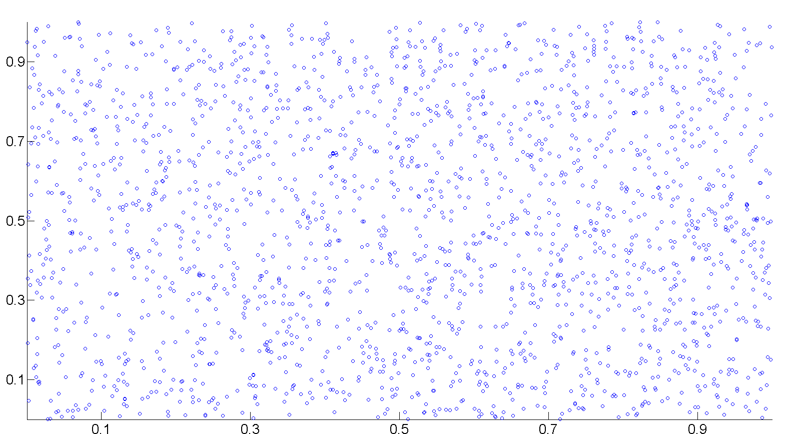
For the numerical example of the process described in Section 3, we consider the Brownian motion (θi1,θi2)=(wi1,wi2),i=1,,2000formulae-sequencesubscriptsuperscript𝜃1𝑖subscriptsuperscript𝜃2𝑖subscriptsuperscript𝑤1𝑖subscriptsuperscript𝑤2𝑖𝑖12000(\theta^{1}_{i},\theta^{2}_{i})=(w^{1}_{i},w^{2}_{i}),~{}i=1,\ldots,2000, in the unit square [0,1]×[0,1]0101[0,1]\times[0,1] with a normal reflection at the boundary. Furthermore, the interferences 𝝍i,li=1,,2000subscript𝝍𝑖𝑙𝑖12000{\boldsymbol{\psi}}_{i,l}~{}i=1,\ldots,2000, are Brownian motion in the interval [0,1]01[0,1] with a normal reflection at the boundary. The n=2000𝑛2000n=2000 data points are sampled uniformly from the unit square as depicted in Fig. 5.1. The intrinsic parameters 𝜽isubscript𝜽𝑖{\boldsymbol{\theta}}_{i} are measured via the set of ζ𝜁\zeta views where ζ=1,,10𝜁110\zeta=1,\ldots,10. Each view is a function of the consensus 𝜽isubscript𝜽𝑖{\boldsymbol{\theta}}_{i} and a function of an additional view-specific Itô process given by 𝝍i,lsubscript𝝍𝑖𝑙{\boldsymbol{\psi}}_{i,l}, 1lζ1𝑙𝜁1\leq l\leq\zeta, that are considered as interferences.
Refer to caption

θi2superscriptsubscript𝜃𝑖2\theta_{i}^{2} θi1superscriptsubscript𝜃𝑖1\theta_{i}^{1}

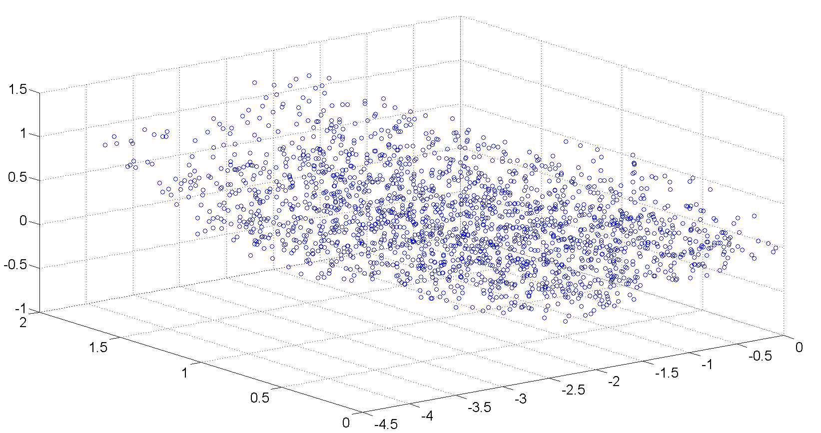
Figure 5.1: The intrinsic parameters 𝜽i,i=1,,2000formulae-sequencesubscript𝜽𝑖𝑖12000{\boldsymbol{\theta}}_{i},~{}i=1,\ldots,2000, of the data.
Refer to caption

x~i,l1superscriptsubscript~𝑥𝑖𝑙1\widetilde{x}_{i,l}^{1}~{}~{}~{}~{}~{}~{}~{}~{}~{}~{}~{}~{}~{}~{}~{}~{}~{}~{}~{}~{}~{}~{}~{}~{}~{}~{}~{}~{}~{}~{}~{}~{} x~i,l2superscriptsubscript~𝑥𝑖𝑙2\widetilde{x}_{i,l}^{2} x~i,l3superscriptsubscript~𝑥𝑖𝑙3\widetilde{x}_{i,l}^{3}

Figure 5.2: A transformed 𝜽isubscript𝜽𝑖{\boldsymbol{\theta}}_{i} from a specific view 𝐱~i,lsubscript~𝐱𝑖𝑙\widetilde{{\bf x}}_{i,l} according to Eq. 5.1

We measure each view 𝐱~i,l,i=1,,2000formulae-sequencesubscript~𝐱𝑖𝑙𝑖12000\widetilde{{\bf x}}_{i,l},~{}i=1,\ldots,2000, through a non-linear transformation by

x~i,l1=a1,1,l(θi1)b1,1,l+a1,2,l(θi2)b1,2,l+a1,3,l(ψi,l)b1,3,lsubscriptsuperscript~𝑥1𝑖𝑙subscript𝑎11𝑙superscriptsuperscriptsubscript𝜃𝑖1subscript𝑏11𝑙subscript𝑎12𝑙superscriptsuperscriptsubscript𝜃𝑖2subscript𝑏12𝑙subscript𝑎13𝑙superscriptsubscript𝜓𝑖𝑙subscript𝑏13𝑙\displaystyle\widetilde{x}^{1}_{i,l}=a_{1,1,l}(\theta_{i}^{1})^{b_{1,1,l}}+a_{1,2,l}(\theta_{i}^{2})^{b_{1,2,l}}+a_{1,3,l}(\psi_{i,l})^{b_{1,3,l}} (5.1)
x~i,l2=a2,1,l(θi1)b2,1,l+a2,2,l(θi2)b2,2,l+a2,3,l(ψi,l)b2,3,lsubscriptsuperscript~𝑥2𝑖𝑙subscript𝑎21𝑙superscriptsuperscriptsubscript𝜃𝑖1subscript𝑏21𝑙subscript𝑎22𝑙superscriptsuperscriptsubscript𝜃𝑖2subscript𝑏22𝑙subscript𝑎23𝑙superscriptsubscript𝜓𝑖𝑙subscript𝑏23𝑙\displaystyle\widetilde{x}^{2}_{i,l}=a_{2,1,l}(\theta_{i}^{1})^{b_{2,1,l}}+a_{2,2,l}(\theta_{i}^{2})^{b_{2,2,l}}+a_{2,3,l}(\psi_{i,l})^{b_{2,3,l}}
x~i,l3=a3,1,l(θi1)b3,1,l+a3,2,l(θi2)b3,2,l+a3,3,l(ψi,l)b3,3,l,subscriptsuperscript~𝑥3𝑖𝑙subscript𝑎31𝑙superscriptsuperscriptsubscript𝜃𝑖1subscript𝑏31𝑙subscript𝑎32𝑙superscriptsuperscriptsubscript𝜃𝑖2subscript𝑏32𝑙subscript𝑎33𝑙superscriptsubscript𝜓𝑖𝑙subscript𝑏33𝑙\displaystyle\widetilde{x}^{3}_{i,l}=a_{3,1,l}(\theta_{i}^{1})^{b_{3,1,l}}+a_{3,2,l}(\theta_{i}^{2})^{b_{3,2,l}}+a_{3,3,l}(\psi_{i,l})^{b_{3,3,l}},

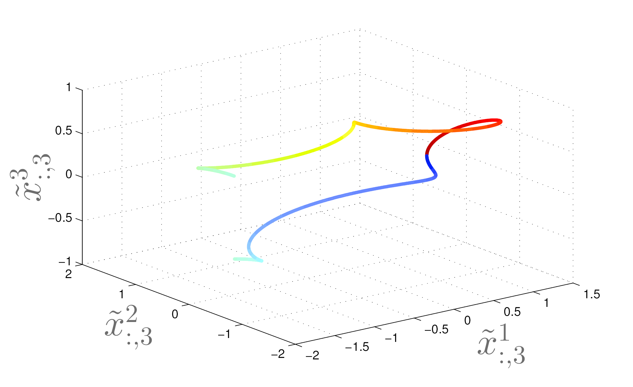
where l=1,,ζ𝑙1𝜁l=1,\ldots,\zeta and ak,q,l0subscript𝑎𝑘𝑞𝑙0a_{k,q,l}\neq 0 is random number chosen uniformly from the interval [2,2]22[-2,2], k,q=1,,3formulae-sequence𝑘𝑞13k,q=1,\ldots,3. Furthermore, bk,q,lsubscript𝑏𝑘𝑞𝑙b_{k,q,l} was fixed to 333. We call 𝐱~i,l=(x~i,l1,x~i,l2,x~i,l3)subscript~𝐱𝑖𝑙subscriptsuperscript~𝑥1𝑖𝑙subscriptsuperscript~𝑥2𝑖𝑙subscriptsuperscript~𝑥3𝑖𝑙\widetilde{{\bf x}}_{i,l}=(\widetilde{x}^{1}_{i,l},\widetilde{x}^{2}_{i,l},\widetilde{x}^{3}_{i,l}), 1i20001𝑖20001\leq i\leq 2000, the observable sample from the space of the l𝑙lth view. This sample is a function of the unknown controlling parameters θi1subscriptsuperscript𝜃1𝑖\theta^{1}_{i} and θi2subscriptsuperscript𝜃2𝑖\theta^{2}_{i} and the unknown interference ψi,lsubscript𝜓𝑖𝑙\psi_{i,l} where 𝐱~i,l=𝐟l(θi1,θi2,ψi,l)subscript~𝐱𝑖𝑙subscript𝐟𝑙subscriptsuperscript𝜃1𝑖subscriptsuperscript𝜃2𝑖subscript𝜓𝑖𝑙\widetilde{{\bf x}}_{i,l}={\bf f}_{l}(\theta^{1}_{i},\theta^{2}_{i},\psi_{i,l}). An illustration of 𝐱~i,lsubscript~𝐱𝑖𝑙\widetilde{{\bf x}}_{i,l} for a specific view is given in Fig. 5.2. The specific instances of the parameters of the transformation (Eq. 5.1), which are used in Fig. 5.2, are

x~i,l1subscriptsuperscript~𝑥1𝑖𝑙\displaystyle\widetilde{x}^{1}_{i,l} =1.94(θi1)3+0.24(θi2)30.62(ψi,l)3absent1.94superscriptsuperscriptsubscript𝜃𝑖130.24superscriptsuperscriptsubscript𝜃𝑖230.62superscriptsubscript𝜓𝑖𝑙3\displaystyle=-1.94(\theta_{i}^{1})^{3}+0.24(\theta_{i}^{2})^{3}-0.62(\psi_{i,l})^{3} (5.2)
x~i,l2subscriptsuperscript~𝑥2𝑖𝑙\displaystyle\widetilde{x}^{2}_{i,l} =1.59(θi1)3+1.39(θi2)3+0.53(ψi,l)3absent1.59superscriptsuperscriptsubscript𝜃𝑖131.39superscriptsuperscriptsubscript𝜃𝑖230.53superscriptsubscript𝜓𝑖𝑙3\displaystyle=-1.59(\theta_{i}^{1})^{3}+1.39(\theta_{i}^{2})^{3}+0.53(\psi_{i,l})^{3}
x~i,l3subscriptsuperscript~𝑥3𝑖𝑙\displaystyle\widetilde{x}^{3}_{i,l} =0.68(θi1)3+0.34(θi2)3+1.10(ψi,l)3.absent0.68superscriptsuperscriptsubscript𝜃𝑖130.34superscriptsuperscriptsubscript𝜃𝑖231.10superscriptsubscript𝜓𝑖𝑙3\displaystyle=-0.68(\theta_{i}^{1})^{3}+0.34(\theta_{i}^{2})^{3}+1.10(\psi_{i,l})^{3}.

Hence, the input data to Algorithm 3.1 is the concatenation of (x~i,l1,x~i,l2,x~i,l3)subscriptsuperscript~𝑥1𝑖𝑙subscriptsuperscript~𝑥2𝑖𝑙subscriptsuperscript~𝑥3𝑖𝑙(\widetilde{x}^{1}_{i,l},\widetilde{x}^{2}_{i,l},\widetilde{x}^{3}_{i,l}) ζ𝜁\zeta times such that 𝐱i=l=1ζ𝐱~i,lsubscript𝐱𝑖superscriptsubscript𝑙1𝜁subscript~𝐱𝑖𝑙{\bf x}_{i}=\cup_{l=1}^{\zeta}\widetilde{{\bf x}}_{i,l}. Algorithm 3.1 was applied to estimate the pairwise intrinsic distances between data points of the consensus. Initially, we run Nc=20000subscript𝑁𝑐20000N_{c}=20000 stochastic simulations for a short time period dt=0.005𝑑𝑡0.005dt=0.005 that were initiated at point 𝜽isubscript𝜽𝑖{\boldsymbol{\theta}}_{i}. The result of the Ncsubscript𝑁𝑐N_{c} stochastic simulations is a point-cloud in the neighborhood of 𝜽isubscript𝜽𝑖{\boldsymbol{\theta}}_{i}. Each point-cloud is mapped using the transformation in Eq. 5.1 to a point-cloud in the neighborhood of 𝐱~i,lsubscript~𝐱𝑖𝑙\widetilde{{\bf x}}_{i,l} in the measured space. Following Eq. 3.11, we calculate the 3×3333\times 3 sample covariance matrix for the point-cloud of each data point in each view. Then, the Mahalanobis distance from Eq. 3.23 is used to estimate the pairwise distances between intrinsic data points in the consensus plus an interference contributed factor. The minimal Mahalanobis distance (over the views) is used to estimate the pairwise distance between intrinsic data points of the consensus 𝜽isubscript𝜽𝑖{\boldsymbol{\theta}}_{i} and 𝜽jsubscript𝜽𝑗{\boldsymbol{\theta}}_{j} i,j=1,,nformulae-sequence𝑖𝑗1𝑛i,j=1,\ldots,n, by

K^ε(𝜽i,𝜽j)min1lζ{exp𝜽i𝜽j2𝝍i,l𝝍j,l2ε},subscript^𝐾𝜀subscript𝜽𝑖subscript𝜽𝑗subscript1𝑙𝜁superscriptnormsubscript𝜽𝑖subscript𝜽𝑗2superscriptnormsubscript𝝍𝑖𝑙subscript𝝍𝑗𝑙2𝜀\hat{K}_{\varepsilon}({\boldsymbol{\theta}}_{i},{\boldsymbol{\theta}}_{j})\approx\min_{1\leq l\leq\zeta}\left\{\exp{\frac{-||{\boldsymbol{\theta}}_{i}-{\boldsymbol{\theta}}_{j}||^{2}-||{\boldsymbol{\psi}}_{i,l}-{\boldsymbol{\psi}}_{j,l}||^{2}}{\varepsilon}}\right\}, (5.3)

for several ε𝜀\varepsilon values. According to Proposition 3.2, when more views are given, the accuracy of the estimated pair-wise affinities improves. Let Kε(𝜽i,𝜽j)=exp𝜽i𝜽j2εsubscript𝐾𝜀subscript𝜽𝑖subscript𝜽𝑗superscriptnormsubscript𝜽𝑖subscript𝜽𝑗2𝜀K_{\varepsilon}({\boldsymbol{\theta}}_{i},{\boldsymbol{\theta}}_{j})=\exp{\frac{-||{\boldsymbol{\theta}}_{i}-{\boldsymbol{\theta}}_{j}||^{2}}{\varepsilon}} be the inaccessible and anisotropic ground truth kernel. The quality factor Q𝑄Q of the Kεsubscript𝐾𝜀K_{\varepsilon} approximation of K^εsubscript^𝐾𝜀\hat{K}_{\varepsilon} is measured by the relative error in Frobenius norm

Q=KεK^εFK^εF.𝑄subscriptnormsubscript𝐾𝜀subscript^𝐾𝜀𝐹subscriptnormsubscript^𝐾𝜀𝐹Q=\frac{||K_{\varepsilon}-\hat{K}_{\varepsilon}||_{F}}{||\hat{K}_{\varepsilon}||_{F}}. (5.4)

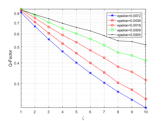
Figure 5.3 displays the relation between the number of views and the approximation quality factor Q𝑄Q of the kernel estimation for several ε𝜀\varepsilon values. The Q𝑄Q-Factor becomes smaller with increasing ε𝜀\varepsilon since KεFsubscriptnormsubscript𝐾𝜀𝐹||K_{\varepsilon}||_{F} grows faster than KεK^εFsubscriptnormsubscript𝐾𝜀subscript^𝐾𝜀𝐹||K_{\varepsilon}-\hat{K}_{\varepsilon}||_{F}. This is the result of a reduced noise contribution 𝝍i,l𝝍j,l2/εsuperscriptnormsubscript𝝍𝑖𝑙subscript𝝍𝑗𝑙2𝜀||{\boldsymbol{\psi}}_{i,l}-{\boldsymbol{\psi}}_{j,l}||^{2}/\varepsilon in Eq. 5.3 as ε𝜀\varepsilon grows while KεFsubscriptnormsubscript𝐾𝜀𝐹||K_{\varepsilon}||_{F} and K^εFsubscriptnormsubscript^𝐾𝜀𝐹||\hat{K}_{\varepsilon}||_{F} grow larger.

Refer to caption

Figure 5.3: Q-factor as a function of ζ𝜁\zeta. For each value of ζ𝜁\zeta, the average accuracy is computed over 202020 simulation repetitions for several ε𝜀\varepsilon values.

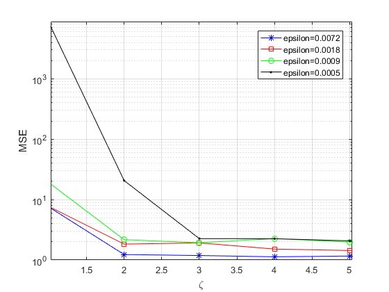
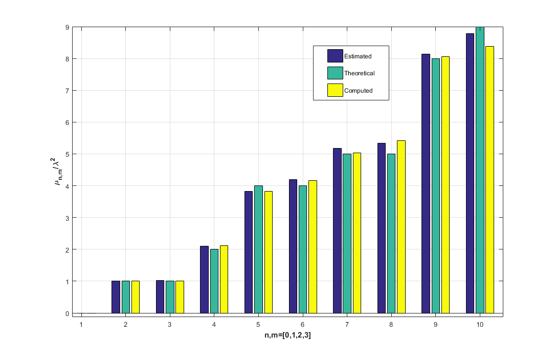
According to [41], the anisotropic kernel Kεsubscript𝐾𝜀K_{\varepsilon} converges to Fokker- Planck operator. Hence, D1Kεε2Lsuperscript𝐷1subscript𝐾𝜀𝜀2𝐿D^{-1}K_{\varepsilon}\approx-\frac{\varepsilon}{2}L, where D𝐷D is a diagonal matrix with [D]ii=j=1nKε(𝜽i,𝜽j)subscriptdelimited-[]𝐷𝑖𝑖superscriptsubscript𝑗1𝑛subscript𝐾𝜀subscript𝜽𝑖subscript𝜽𝑗\left[D\right]_{ii}=\sum_{j=1}^{n}{K}_{\varepsilon}({\boldsymbol{\theta}}_{i},{\boldsymbol{\theta}}_{j}) and L𝐿L is the Fokker -Planck operator of the parametric manifold θi1superscriptsubscript𝜃𝑖1\theta_{i}^{1} and θi2superscriptsubscript𝜃𝑖2\theta_{i}^{2} in Fig. 5.1. From the definition of 𝜽isubscript𝜽𝑖{\boldsymbol{\theta}}_{i}, in this example, the parametric manifold is the unit square with a uniform density, so that L𝐿L is the Laplacian of the unit square whose eigenvalues (for the Neumann boundary conditions) are μn,m=π2(n2+m2),n,m=0,1,formulae-sequencesubscript𝜇𝑛𝑚superscript𝜋2superscript𝑛2superscript𝑚2𝑛𝑚01\mu_{n,m}=\pi^{2}\left(n^{2}+m^{2}\right),~{}n,m=0,1,\ldots. Therefore, the eigenvalues λisubscript𝜆𝑖\lambda_{i} of the row stochastic matrix D1Kεsuperscript𝐷1subscript𝐾𝜀D^{-1}K_{\varepsilon} are given by λieε2μn,msubscript𝜆𝑖superscript𝑒𝜀2subscript𝜇𝑛𝑚\lambda_{i}\approx e^{-\frac{\varepsilon}{2}\mu_{n,m}}. Figure 5.5 shows the values of 2log(λi)/(π2ε),i=1,,10formulae-sequence2subscript𝜆𝑖superscript𝜋2𝜀𝑖110-2\log\left(\lambda_{i}\right)/\left(\pi^{2}\varepsilon\right),~{}i=1,\ldots,10, for the approximated D^1K^εsuperscript^𝐷1subscript^𝐾𝜀\hat{D}^{-1}\hat{K}_{\varepsilon}, where D^^𝐷\hat{D} is a diagonal matrix and [D^]ii=j=1nK^ε(𝜽i,𝜽j)subscriptdelimited-[]^𝐷𝑖𝑖superscriptsubscript𝑗1𝑛subscript^𝐾𝜀subscript𝜽𝑖subscript𝜽𝑗\left[\hat{D}\right]_{ii}=\sum_{j=1}^{n}\hat{K}_{\varepsilon}({\boldsymbol{\theta}}_{i},{\boldsymbol{\theta}}_{j}). The approximation accuracy of the spectral lines n2+m2=[0,1,1,2,4,4,5,5,8,9]superscript𝑛2superscript𝑚20112445589n^{2}+m^{2}=\left[0,1,1,2,4,4,5,5,8,9\right] are shown in Figs 5.4 and 5.5. Figure 5.4 presents the Minimum Squared Error (MSE) between the theoretical spectral lines and the approximated ones as a function of ζ𝜁\zeta, where the approximated λii=1,,10subscript𝜆𝑖𝑖110\lambda_{i}~{}i=1,\ldots,10, were computed using the multi-view scheme of Algorithm 3.1 for several ε𝜀\varepsilon values averaged over 202020 randomization of the transformation from Eq. 5.1. As seen in Fig. 5.4, the accuracy improves significantly when the number of views increases from 111 to 222 views and from 222 views to 333 views. Figure 5.5 compares the estimated spectral lines n2+m2superscript𝑛2superscript𝑚2n^{2}+m^{2} using 101010 views with the theoretical ones and the computed ones using Kεsubscript𝐾𝜀K_{\varepsilon} directly. Figure 5.5 shows that although the parametric manifold was sampled in the presence of noise and an unknown non-linear transformation, the approximation is done with relatively small MSE of 0.550.550.55 between the estimated spectral lines and the theoretical one when the first non-zero spectral line is normalized to 111.

Refer to caption
Figure 5.4: MSE of the Foker-Plank eigenvalues on the unit square in the presence of noisy multi-view process as a function of ε𝜀\varepsilon.
Refer to caption
Figure 5.5: Recovery of the Foker-Plank eigenvalues on the unit square in the presence of noisy multi-view process: theoretical spectral lines (green), the approximated spectral lines (blue) and the computed spectral lines using Kεsubscript𝐾𝜀K_{\varepsilon} (yellow), ε=0.0072𝜀0.0072\varepsilon=0.0072

5.2 Multi-views with an accessible covariance matrix: Example II

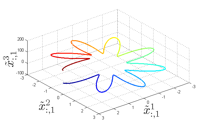
Prior to performance demonstration of Algorithm 4.1, we evaluate the approximation of the Mahalanobis distance in the inaccessible feature space using Eq. 4.2. First, we generate a 333-dimensional manifold using the following equation

Helix : 𝐱~i,1=[x~i,11x~i,12x~i,13]=[f11(θi)f12(θi)f13(θi)]=[(2+cos(8θi))cos(θi)(2+cos(8θi))sin(θi)(3θi2θi)],Helix : subscript~𝐱𝑖1matrixsubscriptsuperscript~𝑥1𝑖1subscriptsuperscript~𝑥2𝑖1subscriptsuperscript~𝑥3𝑖1matrixsubscriptsuperscript𝑓11subscript𝜃𝑖subscriptsuperscript𝑓21subscript𝜃𝑖subscriptsuperscript𝑓31subscript𝜃𝑖matrix28subscript𝜃𝑖subscript𝜃𝑖28subscript𝜃𝑖subscript𝜃𝑖3superscriptsubscript𝜃𝑖2subscript𝜃𝑖\text{Helix : }\widetilde{{\bf x}}_{i,1}=\begin{bmatrix}{\widetilde{x}^{1}_{i,1}}\\ {\widetilde{x}^{2}_{i,1}}\\ {\widetilde{x}^{3}_{i,1}}\\ \end{bmatrix}=\begin{bmatrix}{f^{1}_{1}}(\theta_{i})\\ {f^{2}_{1}}(\theta_{i})\\ {f^{3}_{1}}(\theta_{i})\\ \end{bmatrix}=\begin{bmatrix}{(2+\cos(8\theta_{i}))\cdot\cos(\theta_{i})}\\ {(2+\cos(8\theta_{i}))\cdot\sin(\theta_{i})}\\ {(3\theta_{i}^{2}-\theta_{i})}\\ \end{bmatrix}, (5.5)

where the intrinsic governing parameters θisubscript𝜃𝑖\theta_{i}, i=1,,n=20,000formulae-sequence𝑖1𝑛20000i=1,\ldots,n=20,000, are generated by θisubscript𝜃𝑖\theta_{i} that are uniformly drawn from [0,2π]02𝜋[0,2\pi]. The generated manifold is presented in Fig. 5.6.
Refer to caption
Figure 5.6: The sampled helix (Eq. 5.5)
Refer to caption
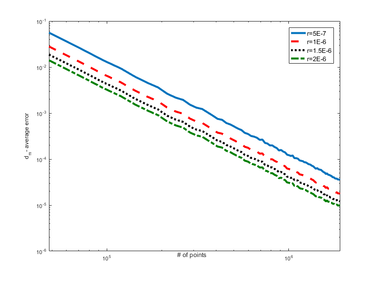
Figure 5.7: The average error between the Mahalanobis distances in the ambient space and the corresponding Mahalanobis distances in the parametric space as a function of the number of points per unit length generated in the parametric space. The value r𝑟r, represents the maximal distance that is used to find neighbors for the covariance matrix estimation.

The empirical covariance matrix in Eq. 4.1 depends on the neighbors of each data point. Denote by εr>0subscript𝜀𝑟0\varepsilon_{r}>0 the neighborhood radius used by the covariance matrix computation at each data point. The approximation average error in Eq. 4.1 is presented in Fig. 5.7, where the average is taken over 100100100 repeated simulations. It is evident that the errors for both datasets diminish as εrsubscript𝜀𝑟\varepsilon_{r} grows and the number of neighbors increases. As a result, the covariance matrix approximation improves and with it the similarity between both Mahalanobis distances in the ambient space. The corresponding Mahalanobis distances in the parametric space are improved.

In the rest of this section, the approximation of the affinity measure is evaluated. ζ=10𝜁10\zeta=10 views are generated to evaluate the performance of Algorithm 4.1. All the views are 333-dimensional that are based on one underlying angular parameter denoted by θi,i=1,,nformulae-sequencesubscript𝜃𝑖𝑖1𝑛\theta_{i}\in{\mathbbm{R}},~{}i=1,\ldots,n. The 101010 views are generated by the application of the following function

Helix III: 𝐱~i,l=[x~i,l1x~i,l2x~i,l3]=[fl1(𝜽i)fl2(𝜽i)fl3(𝜽i)]=[(4/3)cos(𝜽i+Zl1)(1/3)cos(4(𝜽i+Zl1))(4/3)sin(𝜽i+Zl2)(1/3)sin(4(𝜽i+Zl2))sin(0.8mod((𝜽i+Zl3),2π))],\text{Helix III: }\widetilde{{\bf x}}_{i,l}=\begin{bmatrix}{\widetilde{x}_{i,l}^{1}}\\ {\widetilde{x}_{i,l}^{2}}\\ {\widetilde{x}_{i,l}^{3}}\\ \end{bmatrix}=\begin{bmatrix}{f_{l}^{1}}({\boldsymbol{\theta}}_{i})\\ {f_{l}^{2}}({\boldsymbol{\theta}}_{i})\\ {f_{l}^{3}}({\boldsymbol{\theta}}_{i})\\ \end{bmatrix}=\begin{bmatrix}{(4/3)\cdot\cos({\boldsymbol{\theta}}_{i}+Z_{l}^{1})-(1/3)\cdot\cos(4({\boldsymbol{\theta}}_{i}+Z_{l}^{1}))}\\ {(4/3)\cdot\sin({\boldsymbol{\theta}}_{i}+Z_{l}^{2})-(1/3)\cdot\sin(4({\boldsymbol{\theta}}_{i}+Z_{l}^{2}))}\\ {\sin(0.8\cdot\mod(({\boldsymbol{\theta}}_{i}+Z_{l}^{3}),2\pi))}\\ \end{bmatrix}, (5.6)

where Zl1,Zl2,Zl3,1l10superscriptsubscript𝑍𝑙1superscriptsubscript𝑍𝑙2superscriptsubscript𝑍𝑙31𝑙10Z_{l}^{1},Z_{l}^{2},Z_{l}^{3},1\leq l\leq 10, are random variables drawn from a uniform distribution on the interval [0,2π]02𝜋[0,2\pi]. As demonstrated in Fig. 5.8, each view is a deformation of an open flower-shaped manifold. A similar deformation can occur in various real-life applications where the measured data is the output from some non-linear phenomena. In this experiment, we demonstrate the ability of a multi-view approach to overcome such deformations.
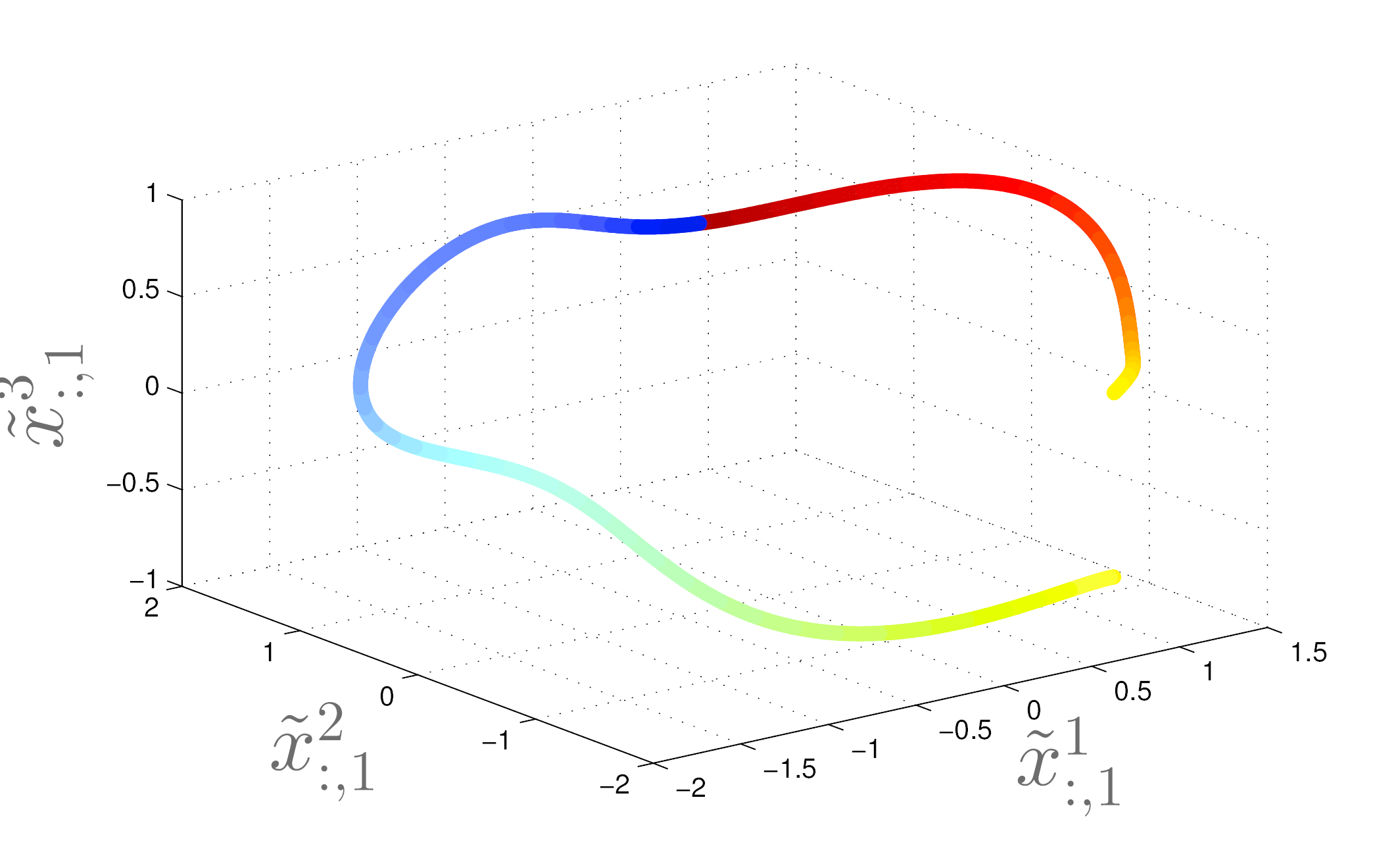
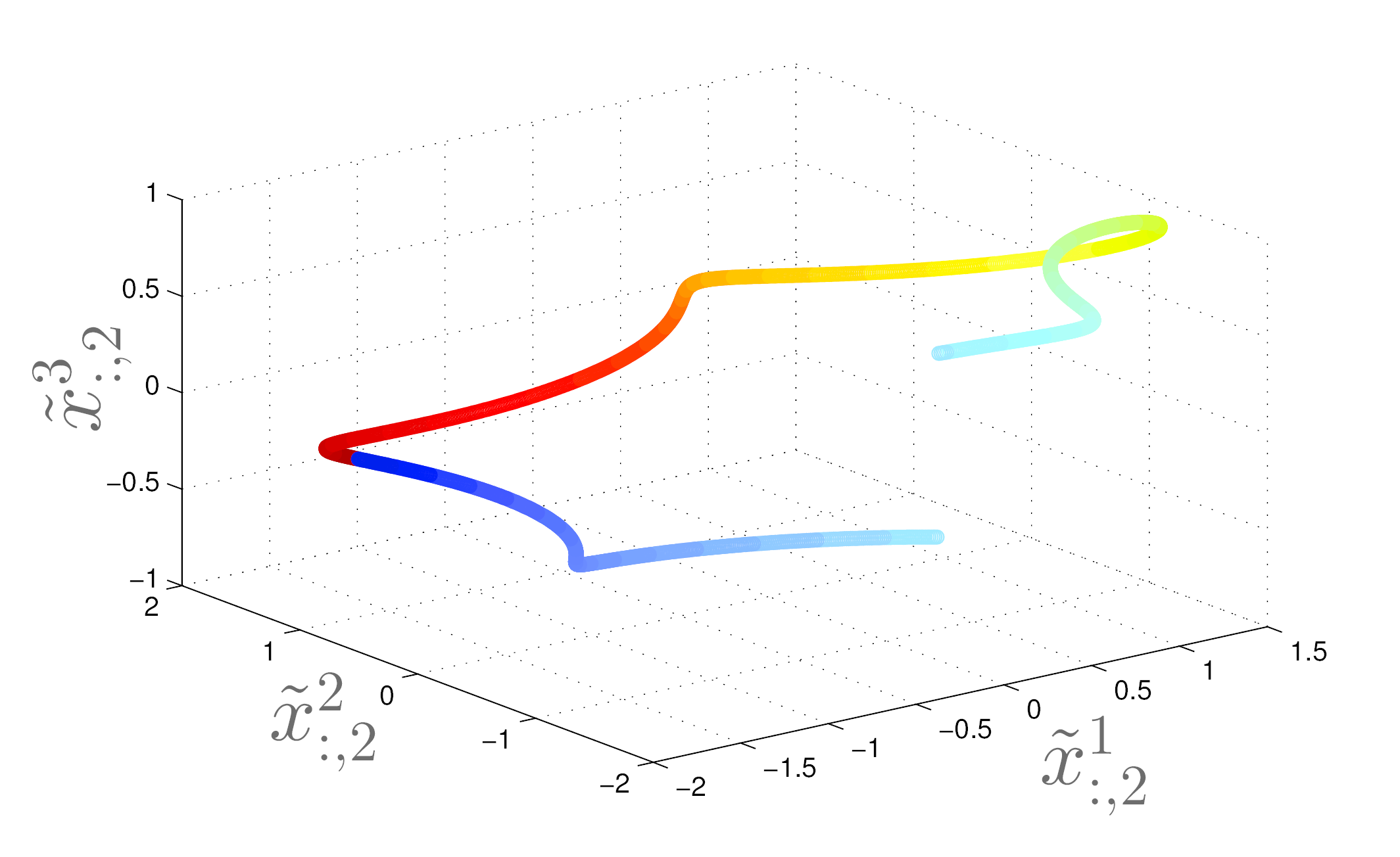
Refer to caption
(a) View I
Refer to caption
(b) View II
Refer to caption
(c) View III
Figure 5.8: The three manifolds generated by Eq. 5.6.

To extract the underlying parameter θisubscript𝜃𝑖\theta_{i}, we first apply the DM to each view. The two leading coordinates of the extracted embedding are denoted by ϕ1subscriptitalic-ϕ1\phi_{1} and ϕ2subscriptitalic-ϕ2\phi_{2}. They are presented in Fig. 5.9. All the extracted manifolds are horseshoe shapes that consist of a large gap created by the deformation (Eq. 5.6) in the third coordinate of the sampled data.
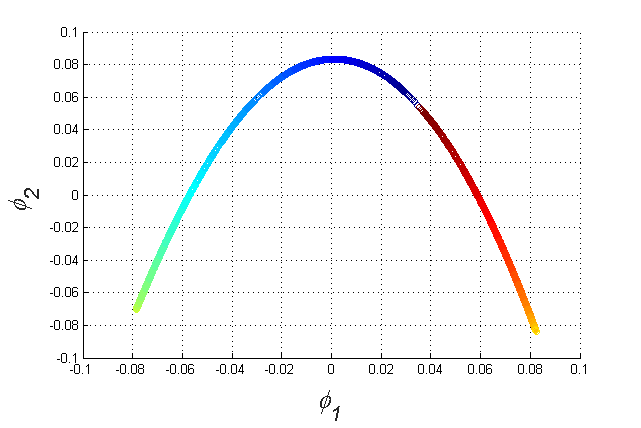
Refer to caption
(a) DM of View I
Refer to caption
(b) DM of View II
Refer to caption
(c) DM of View III
Figure 5.9: The DM embedding of each single view l=1,,3𝑙13l=1,\dots,3.

Next, the 101010 available views are concatenated to a single view 𝐱i=[𝐱~i,1,,𝐱~i,10],i=1,,2000formulae-sequencesubscript𝐱𝑖subscript~𝐱𝑖1subscript~𝐱𝑖10𝑖12000{\bf x}_{i}=\left[\widetilde{{\bf x}}_{i,1},\ldots,\widetilde{{\bf x}}_{i,10}\right],~{}i=1,\ldots,2000. The Mahalanobis distance is computed using Eq. 4.1 and DM is applied to the resulted kernel. The first two leading coordinates of the kernel-based DM are presented in Fig. 5.9. The large gap in each of the extracted manifolds is a deformation caused by the third coordinate of the transformation functions 𝐟l(𝜽i)=[fl1(𝜽i),fl2(𝜽i),fl3(𝜽i)]subscript𝐟𝑙subscript𝜽𝑖superscriptsubscript𝑓𝑙1subscript𝜽𝑖superscriptsubscript𝑓𝑙2subscript𝜽𝑖superscriptsubscript𝑓𝑙3subscript𝜽𝑖{\bf f}_{l}({\boldsymbol{\theta}}_{i})=[{f_{l}^{1}}({\boldsymbol{\theta}}_{i}),{f_{l}^{2}}({\boldsymbol{\theta}}_{i}),{f_{l}^{3}}({\boldsymbol{\theta}}_{i})] (Eq. 5.6). Furthermore, the output from the application of DM to the concatenation of the 101010 views is presented in Fig. 5.10(a). The embedded manifold is even more distorted as the gaps in the embedding suggests. Hence, the standard procedure, which concatenates the given set of features without considering the specific distortion each subset of features, may result in a distorted embedding.
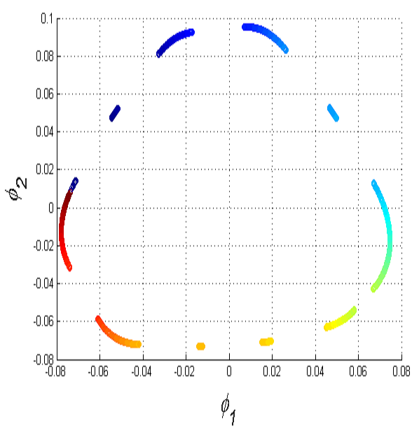
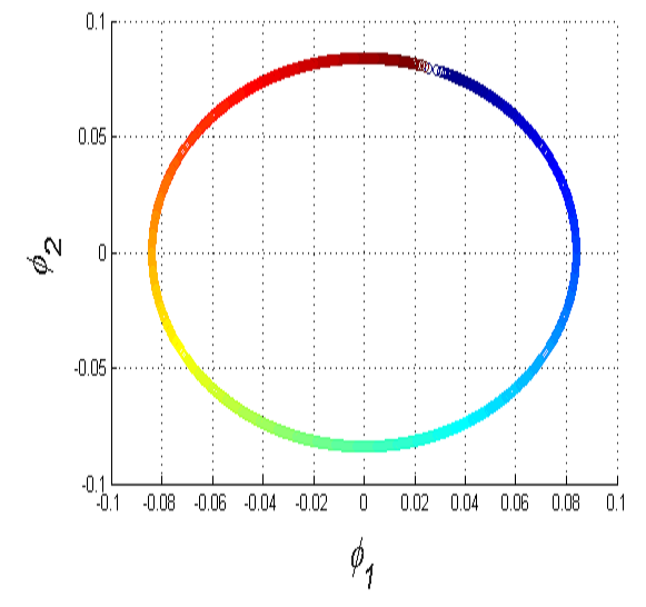
Refer to caption
(a) DM cooredinates of the concatenated views
Refer to caption
(b) DM coordinates of the multi-view-based kernel
Figure 5.10: Concatenation of DM coordinates 𝐱ii=1,,20,000subscript𝐱𝑖𝑖120000{\bf x}_{i}~{}i=1,\ldots,20,000 (a) compared to the DM application to the multi-view kernel approximated by Algorithm 4.1 that considers the views 𝐱~i,l,l=1,,10formulae-sequencesubscript~𝐱𝑖𝑙𝑙110\widetilde{{\bf x}}_{i,l},~{}l=1,\ldots,10 (b).

Finally, we apply Algorithm 4.1 to all 101010 views and compute the two leading DM coordinates. The outputs are presented in Fig. 5.10(b). The algorithm overcomes deformations, seen as gaps in the concatenated embedding, by considering only the non-deformed small distances as the outcome of the majority vote function in Algorithm 4.1. The result is the circle shaped manifold that completely agrees with the corresponding intrinsic controlling angle parameter θisubscript𝜃𝑖\theta_{i}.

5.3 Classification of Seismic Events: Example III

To demonstrate the method in Section 3 for analyzing a real data, we tackle the binary classification problem of seismic events. Discrimination between earthquakes and explosions is an essential component of nuclear test monitoring and it is also essential for creating reliable earthquake catalogs [37]. For this evaluation, we analyzed a dataset containing 464646 earthquakes and 626262 (non-nuclear) explosions recorded in Israel. The labels were annotated by a specialist from the Geophysical Institute of Israel (GII).

Seismic waveforms were recorded simultaneously using 333 channels in two seismic monitoring stations. Each measurement channel is considered as a view to have a total of ζ=6𝜁6\zeta=6 views. Since the seismic monitoring stations are far from each other, local noisy events such as constructions activities or vehicles movements are station specific. A Sonogram [20] is computed from each measurement channel for each seismic event. The Sonogram is a time-frequency representation equally tempered on a logarithmic scale. Each Sonogram spectral component is normalized to have a maximum value of 111. The detailed feature extraction process is given in [37]. An example of a normalized Sonogram representation of an explosion is presented in Fig. 5.11. Under the assumption of Section 3, we consider each of the 666 measurement channels as Itô process. To evaluate Algorithm 3.1 in extracting the consensus from the given measurements, we added a Gaussian noise with zero mean and a variance σNsubscript𝜎𝑁\sigma_{N} to 222 views out of 666. The added noise simulates an interference process that contaminates the two measurement channels. Since this noise is uncorrelated to the interesting seismic event it is not a part in the consensus.
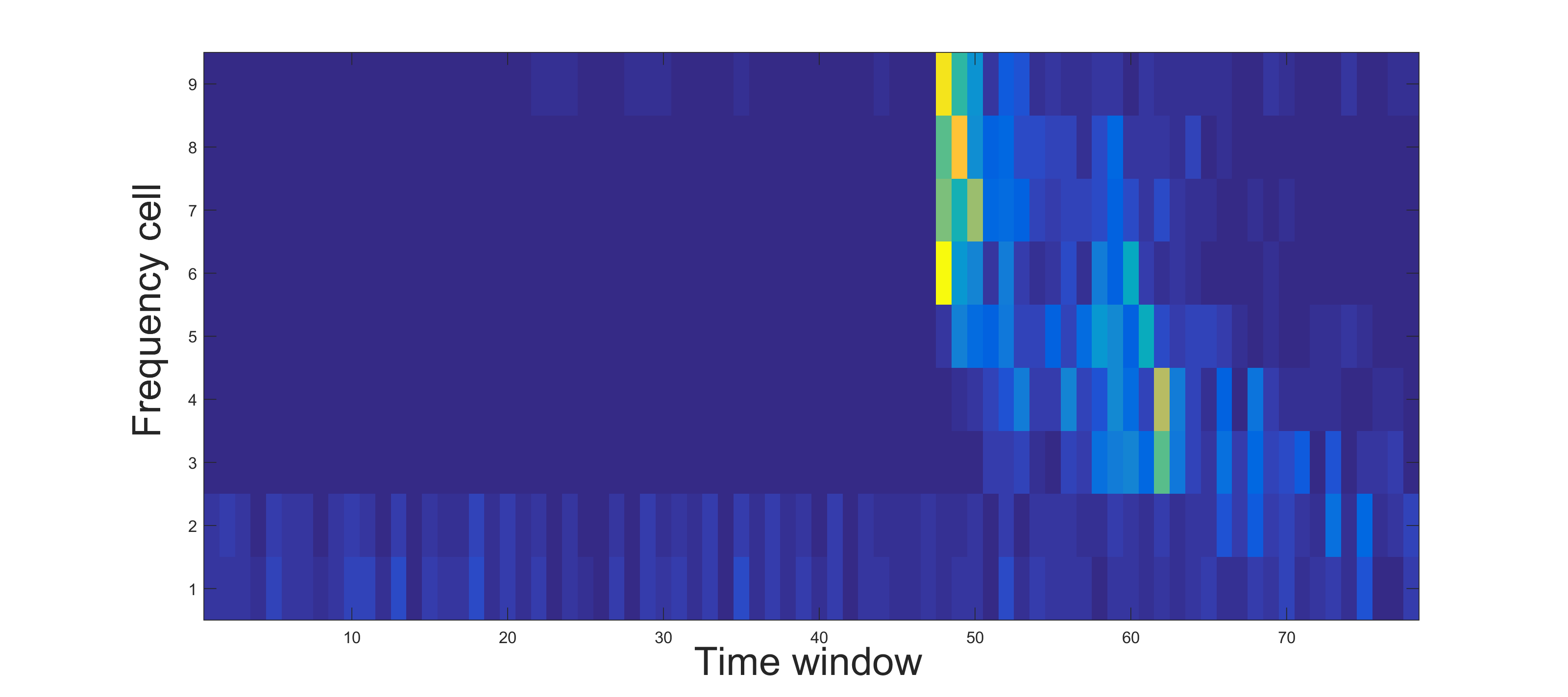
Refer to caption
Figure 5.11: A Sonogram example of an explosion.

Each feature vector 𝒙~i,lsubscript~𝒙𝑖𝑙\tilde{{\mbox{\boldmath$x$}}}_{i,l} represents the spectral properties of i=1,,78𝑖178i=1,...,78 time window for l=1,..,6l=1,..,6 view. Algorithm 3.1 is applied followed by a spectral decomposition of Kϵsubscript𝐾italic-ϵK_{\epsilon}. The first nontrivial eigenvector is used as the representation for each seismic event. A binary classification is performed using K-NN (K=5𝐾5K=5) in a leave-one-out fashion. Furthermore, we applied the multi-view-based DM from [33] and a naive method of DM applied to a concatenation of the feature vectors 𝒙~i,l,l=1,,6formulae-sequencesubscript~𝒙𝑖𝑙𝑙16\tilde{{\mbox{\boldmath$x$}}}_{i,l},l=1,...,6. The comparison between the resulted classification accuracies is presented in Fig. 5.12.
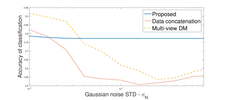
Refer to caption
Figure 5.12: Average classification accuracy of seismic events by Algorithm 3.1 (blue), naive DM (dashed red) and multi-view-based DM [33].

It is evident from Fig. 5.12 that for measurements with a low power noise, the multi-view-based DM from [33] has the best accuracy of 91%percent9191\%. Application of Algorithm 3.1 results in a moderate accuracy of 79%percent7979\%. However, when σNsubscript𝜎𝑁\sigma_{N} is significant, Algorithm 3.1 overcomes the noise and is able to maintain a moderate accuracy while both the naive method and the multi-view-based DM method are failing to less than 60%percent6060\% accuracy. The performance of the proposed method is stable over large spans of noise power due to the availability of at least one reliable view for each classified seismic event.

6 Conclusions

This paper presents a kernel construction scheme by approximating the similarity between intrinsic parameters that are common to multiple subset of features (also called views) in the presence of noise and non-linear transformation of the inaccessible controlling parameters. The presented method utilizes the relation between the Jacobian of each view and the corresponding Mahalanobis distance when a local covariance is approximated. This relation enables to approximate the affinities between intrinsic controlling parameters by considering the Mahalanobis distance of each view. The constructed kernel can be further normalized and decomposed to find an embedding of the data. In order to demonstrate the effectiveness of the proposed method, we analyzed several synthetic datasets. This analysis showed that the correct affinities can be approximated in the presence of significant noise and a unknown non-linear transformation. Furthermore, in cases where the features are the output of a transformed intrinsic parameters with an associated non-full rank Jacobian, then the concatenation of the entire set of features results in a deformed manifold. In this case, the proposed multi-view scheme overcomes the problematic Jacobian and outputs a non-deformed manifold. The proposed methodology involves a single spectral decomposition while increasing the number of (smaller Covariance-based) Mahalanobis distances computations per affinity. Hence, the growth in computation complexity is negligible.

Acknowledgment

This research was partially supported by Indo-Israel CollAborative for Infrastructure Security (Grant No. 1), Israel Science Foundation (Grant No. 1556/17), US-Israel Binational Science Foundation (BSF 2012282), Len Blavatnik and the Blavatnik Family Foundation, Blavatink ICRC Funds. The third author was partially supported by Fellowships from Jyväskylä University and the Clore Foundation. We also would like to thank Aviv Rotbart for assisting with the experimental results.

References

  • [1] S. Akaho. A kernel method for canonical correlation analysis. arXiv preprint cs/0609071, 2006.
  • [2] M. Belkin and P. Niyogi. Laplacian eigenmaps for dimensionality reduction and data representation. Neural Computation, 15(6):1373–1396, 2003.
  • [3] T. Berry and J. Harlim. Iterated diffusion maps for feature identification. In Press, Applied and Computational Harmonic Analysis, 2016.
  • [4] T. Berry and T. Sauer. Local kernels and the geometric structure of data. Applied and Computational Harmonic Analysis, 40(3):439 – 469, 2016.
  • [5] B. Boots and G. Gordon. Two-manifold problems with applications to nonlinear system identication. In Proc. 29th Intl. Conf. on Machine Learning (ICML), 2012.
  • [6] F. Camastra. Data dimensionality estimation methods: a survey. Pattern recognition, 36(12):2945–2954, 2003.
  • [7] C. Ceruti, S. Bassis, A. Rozza, G. Lombardi, E. Casiraghi, and P. Campadelli. Danco: An intrinsic dimensionality estimator exploiting angle and norm concentration. Pattern Recognition, 47(8):2569 – 2581, 2014.
  • [8] K. Chadhuri, S. M. Kakade, K. Livescu, and K. Sridharan. Multi-view clustering via canonical correlation analysis. In Proc. 26th Intl. Conf. on Machine Learning (ICML), pages 126–136, 2009.
  • [9] R. R. Coifman and M. J. Hirn. Diffusion maps for changing data. Applied and Computational Harmonic Analysis, 36(1):79 – 107, 2014.
  • [10] R.R. Coifman and S. Lafon. Diffusion maps. Applied and Computational Harmonic Analysis, 21(1):5–30, 2006.
  • [11] C. Cortes and V. Vapnik. Support-vector networks. Machine Learning, 20(3):273–297, 1995.
  • [12] T. Cox and M. Cox. Multidimensional Scaling. Chapman and Hall, London, UK, 1994.
  • [13] V. R. de Sa. Spectral clustering with two views. In ICML Workshop on Learning with Multiple Views, 2005.
  • [14] D.L. Donoho and C. Grimes. Hessian eigenmaps: New locally linear embedding techniques for high dimensional data. Proceedings of the National Academy of Sciences of the United States of America, 100:5591–5596, May 2003.
  • [15] W. T. Freeman and J. B. Tenenbaum. Learning bilinear models for two-factor problems in vision. In Computer Vision and Pattern Recognition (CVPR), volume 21, pages 554–560, 1997.
  • [16] K. Fukunaga and D. R. Olsen. An algorithm for finding intrinsic dimensionality of data. IEEE Transactions on Computers, 100(2):176–183, 1971.
  • [17] T. Hastie, R. Tibshirani, and J. Friedman. The Elements of Statistical Learning. Springer Series in Statistics. Springer New York Inc., New York, NY, USA, 2001.
  • [18] H. Hotelling. Analysis of a complex of statistical variables into principal components. Journal of Educational Psychology, 24, 1933.
  • [19] I.T. Jolliffe. Principal Component Analysis. Springer, New York, NY, 1986.
  • [20] M. Joswig. Pattern recognition for earthquake detection. Bulletin of the Seismological Society of America, 80(1):170–186, 1990.
  • [21] I. G. Kevrekidis, C. W. Gear, and G. Hummer. Equation-free: The computer-aided analysis of complex multiscale systems. AIChE J., 50(7):1346–1355, 2004.
  • [22] J.B. Kruskal. Multidimensional scaling by optimizing goodness of fit to a nonmetric hypothesis. Psychometrika, 29:1– 27, 1964.
  • [23] A. Kumar, P. Rai, and H. Daume. Co-regularized multi-view spectral clustering. In Advances in Neural Information Processing Systems, volume 24, 2011.
  • [24] D. Kushnir, A. Haddad, and R. R. Coifman. Anisotropic diffusion on sub-manifolds with application to earth structure classification. Applied and Computational Harmonic Analysis, 32(2):280 – 294, 2012.
  • [25] S. Lafon. Diffusion Maps and Geometric Harmonics. PhD thesis, Yale University, May 2004.
  • [26] P. L. Lai and C. Fyfe. Kernel and nonlinear canonical correlation analysis. International Journal of Neural Systems, 10(05):365–377, 2000.
  • [27] R. Lederman, R. Talmon, H.-T. Wu, Y.-L. Lo, and R. Coifman. Alternating diffusion for common manifold learning with application to sleep stage assessment. In 2015 IEEE International Conference on Acoustics, Speech and Signal Processing, ICASSP 2015, South Brisbane, Queensland, Australia, April 19-24, 2015, pages 5758–5762, 2015.
  • [28] R. R. Lederman and R. Talmon. Common manifold learning using alternating-diffusion. Technical report, submitted, Tech. Report YALEU/DCS/TR1497, 2014.
  • [29] R. R. Lederman and R. Talmon. Learning the geometry of common latent variables using alternating-diffusion. Applied and Computational Harmonic Analysis, pages –, 2015.
  • [30] R. T. Li, T.-P. Tian, and S. Sclaroff. Simultaneous learning of nonlinear manifold and dynamical models for high-dimensional time series. In ICCV, pages 1–8. IEEE, 2007.
  • [31] R.-S. Lin, C.-B. Liu, M.-H. Yang, N. Ahuja, and S. Levinson. Learning nonlinear manifolds from time series. In A. Leonardis, H. Bischof, and A. Pinz, editors, Computer Vision ECCV 2006, volume 3952 of Lecture Notes in Computer Science, pages 245–256. Springer Berlin Heidelberg, 2006.
  • [32] O. Lindenbaum, A. Yeredor, and M. Salhov. Learning coupled embedding using multiview diffusion maps. In International Conference on Latent Variable Analysis and Signal Separation, pages 127–134. Springer, 2015.
  • [33] O. Lindenbaum, A. Yeredor, M. Salhov, and A. Averbuch. Multiview diffusion maps. arXiv preprint arXiv:1508.05550, 2015.
  • [34] J. H. Mack, L. Buesing, J. P. Cunningham, B. M. Yu, V. S. Krishna, and M. Sahani. Empirical models of spiking in neural populations. In J. Shawe-Taylor, R.S. Zemel, P.L. Bartlett, F. Pereira, and K.Q. Weinberger, editors, Advances in Neural Information Processing Systems 24, pages 1350–1358. Curran Associates, Inc., 2011.
  • [35] P. C. Mahalanobis. On the generalised distance in statistics. In Proceedings National Institute of Science, India, volume 2, pages 49–55, April 1936.
  • [36] K. W. Pettis, T. A. Bailey, A. K. Jain, and R. C. Dubes. An intrinsic dimensionality estimator from near-neighbor information. IEEE Transactions on pattern analysis and machine intelligence, (1):25–37, 1979.
  • [37] N. Rabin, Y. Bregman, O. Lindenbaum, Y. Ben-Horin, and A. Averbuch. Earthquake-explosion discrimination using diffusion maps. Geophysical Journal International, 207(3):1484–1492, 2016.
  • [38] A. Rahimi, B. Recht, and T. Darrell. Learning appearance manifolds from video. In 2005 IEEE Computer Society Conference on Computer Vision and Pattern Recognition (CVPR 2005), 20-26 June 2005, San Diego, CA, USA, pages 868–875, 2005.
  • [39] S. T. Roweis and K. S. Lawrence. Nonlinear dimensionality reduction by local linear embedding. Science, 290:2323–2326, 2000.
  • [40] A. Singer. Spectral independent component analysis. Applied and Computational Harmonic Analysis, 21(1):135–144, 2006.
  • [41] A. Singer and R.R. Coifman. Non-linear independent component analysis with diffusion maps. Applied and Computational Harmonic Analysis, 25(2):226–239, 2008.
  • [42] A. Singer and H.-t. Wu. Orientability and diffusion maps. Applied and Computational Harmonic Analysis, 31(1):44–58, 2011.
  • [43] AJ. Smola and B. Schölkopf. Bayesian Kernel Methods, volume LNAI 2600, chapter 0, pages 65–117. Springer, Berlin, Germany, 2003.
  • [44] R. Talmon and R. R. Coifman. Intrinsic modeling of stochastic dynamical systems using empirical geometry. Applied and Computational Harmonic Analysis, 39(1):138–160, 2015.
  • [45] J. B. Tenenbaum, V. de Silva, and J. C. Langford. A global geometric framework for nonlinear dimensionality reduction. Science, 290(5500):2319–2323, 2000.
  • [46] G. V. Trunk. Stastical estimation of the intrinsic dimensionality of a noisy signal collection. IEEE Transactions on Computers, 100(2):165–171, 1976.
  • [47] P. J. Verveer and R. P. W. Duin. An evaluation of intrinsic dimensionality estimators. IEEE Transactions on pattern analysis and machine intelligence, 17(1):81–86, 1995.
  • [48] B. Wang, J. Jiang, W. Wang, Z. Zhou, and Z. Tu. Unsupervised metric fusion by cross diffusion. In Computer Vision and Pattern Recognition (CVPR), pages 2997–3004, 2012.
  • [49] G. Yang, X. Xu, and J. Zhang. Manifold alignment via local tangent space alignment. International Conference on Computer Science and Software Engineering, December 2008.
  • [50] Z. Zhang and H. Zha. Principal manifolds and nonlinear dimension reduction via local tangent space alignment. Technical Report CSE-02-019, Department of Computer Science and Engineering, Pennsylvania State University, 2002.
  • [51] D. Zhou and C. J. C. Burges. Spectral clustering and transductive learning with multiple views. Proceedings of the 24th international conference on Machine learning, pages 1159–1166, 2007.