Beyond Linear Fields: the Lie-Taylor Expansion

Abstract

The work extends the linear fields’ solution of compressible nonlinear magnetohydrodynamics (MHD) to the case where the magnetic field depends on superlinear powers of position vector, usually but not always, expressed in Cartesian components. Implications of the resulting Lie-Taylor series expansion for physical applicability of the Dolzhansky-Kirchhoff (D-K) equations are found to be positive. It is demonstrated how resistivity may be included in the D-K model. Arguments are put forward that the D-K equations may be regarded as illustrating properties of nonlinear MHD in the same sense that the Lorenz equations inform about the onset of convective turbulence. It is suggested that the Lie-Taylor series approach may lead to valuable insights into other fluid models.

Wayne Arter

1 Introduction

The recent work [1] showed how the equations of ideal, compressible magnetohydrodynamics may be elegantly formulated in terms of Lie derivatives, building on the work of Helmholtz, Walen and Arnold. The magnetic induction equation for compressible flow may be formulated in terms of a Lie derivative of a vector by introducing the field $\tilde{\bf B}$ defined as the magnetic field ${\bf B}$ divided by the mass density,

$$\frac{\partial\tilde{\bf B}}{\partial t}=\mathcal{L}_{\bf u}(\tilde{\bf B})$$ (1)

where $\mathcal{L}_{\bf u}$ is the Lie derivative with respect to the flow field ${\bf u}$, $\tilde{\bf B}={\bf B}/\rho$ and $\rho$ is mass density. The dynamical, potential vorticity equation [1] may also be put into the Lie derivative form

$$\frac{\partial\tilde{\bm{\omega}}}{\partial t}=\mathcal{R}+{\mathcal{L}}_{\bf u}(\tilde{\bm{\omega}})-{\mathcal{L}}_{\tilde{\bf B}}(\tilde{\bf J})$$ (2)

where the potential vorticity $\tilde{\bm{\omega}}=\nabla\times{\bf u}/\rho$ and the potential current $\tilde{\bf J}=\nabla\times{\bf B}/\rho$. The term $\mathcal{R}$ vanishes either upon making the barotropic assumption that pressure $p(\rho)$ or sometimes in the isentropic approximation. Observe that the vectors which are evolved by Eqs (1) and (2) satisfy $\nabla\cdot(\rho{\bf F})={\bf 0}$, provided there is mass conservation and $\rho{\bf F}$ is solenoidal initially.

Now it is known since Dungey [2] that if the velocity field depends linearly on Cartesian position vector, then compressible MHD is reducible exactly to a set of ordinary differential equations (ODEs) in the coefficients of the proportionality constants. (There is a much longer and complicated history regarding classical hydrodynamics which will not be discussed herein.) This “linear fields" theory has been developed further as described in Arnold & Khesin [3, § I.10.C] to 3-D. Dolzhansky [4] explains clearly how a special choice of 3-D vector basis for both velocity and magnetic field leads to the Kirchhoff equations, a sixth order ODE describing the motion of an ellipsoid immersed in fluid. The difficulty with the 3-D vector basis is that it requires initial current distributions corresponding to the linear magnetic field that are not easy to realise in practice. It is possible to conceive that an ellipsoidal blob of uniform vorticity might somehow appear, indeed an elliptical blob, embedded in a 2-D potential flow was proposed by Helmholtz in 1889 as a model for a tornado [5, § 159]. However, it strains the imagination as to how an isolated ellipsoidal current distribution might be spontaneously produced.

Arter [6] pointed out that the Cartesian linear fields could be regarded as the truncation of a Taylor series expansion solution in position to first order. Thus a problem with boundary conditions at a finite distance from the origin might be formulated, by allowing higher order Taylor terms to help say fix the current on a flat surface at distance $\lambda$ rather than on the problematic ellipsoidal surface. Substituting the higher order terms in the governing partial differential equations (PDEs) leads to complicated sets of ordinary differential equations (ODEs), but fortunately the use of the above Lie derivative form for MHD is especially convenient for such analysis, see the next Section 2. Subsection 3 first discusses implications of the results in Subsection 2.4 of Section 2 for Dolzhansky’s model and then explores important mathematical features of the Dolzhansky-Kirchhoff (D-K) equations. Section 4 discusses the introduction of resistivity into the D-K model and conclusions are drawn in Section 5.

2 Lie-Taylor Expansion and Implications

2.1 Lie Derivative Expansions

Suppose that the vectors ${\bf u}$ and ${\bf q}$ have components labelled $j$ and moreover that each component may be separately expressed as a Taylor series in coordinates $x^{i}$, i.e.

$$u^{j}=U^{j}+U^{j}_{m}x^{m}+U^{j}_{mn}x^{m}x^{n}+U^{j}_{mnq}x^{m}x^{n}x^{q}+\ldots$$ (3)

$$q^{j}=Q^{j}+Q^{j}_{m}x^{m}+Q^{j}_{mn}x^{m}x^{n}+Q^{j}_{mnq}x^{m}x^{n}x^{q}+\ldots$$ (4)

using the Einstein summation convention, and where for example

$$U^{j}_{mn}=\frac{1}{2!}\frac{\partial^{2}u^{j}}{\partial x^{m}\partial x^{n}}$$ (5)

so that the suffices denote normalised derivatives with respect to position coordinate. (More conventional notation would see a comma preceding the suffices and no factorial prefactor, but here would serve to make complicated expressions even longer.) When ${\bf q}$ is set equal to $\tilde{\bf B}$, the evolution of ${\bf q}$ from Eq. (1) may be written

$$\frac{\partial{\bf q}}{\partial t}=[{\bf u},{\bf q}]$$ (6)

since there is the textbook result, see ref [1], that

$${\mathcal{L}}_{\bf v}({\bf w})^{i}=w^{k}\frac{\partial v^{i}}{\partial x^{k}}-v^{k}\frac{\partial w^{i}}{\partial x^{k}}$$ (7)

which serves also to define the commutator $[{\bf v},{\bf w}]$ for general vectors. Hence in component form

$$\frac{\partial q^{j}}{\partial t}=q^{i}\frac{\partial u^{j}}{\partial x^{i}}-u^{i}\frac{\partial q^{j}}{\partial x^{i}}$$ (8)

It follows that it is necessary to calculate the derivative Taylor series:

$$\frac{\partial q^{j}}{\partial x^{k}} = Q^{j}_{m}\delta_{mk}+Q^{j}_{mn}\delta_{mk}x^{n}+Q^{j}_{mn}x^{m}\delta_{rnmk}+$$ (9)

$$+ Q^{j}_{mnq}\delta_{mk}x^{n}x^{q}+Q^{j}_{mnq}x^{m}\delta_{nk}x^{q}+Q^{j}_{mnq}x^{m}x^{n}\delta_{qk}+\ldots$$

which since partial derivatives commute, implying $Q^{j}_{kn}=Q^{j}_{nk}$, gives

$$\frac{\partial q^{j}}{\partial x^{k}}=Q^{j}_{k}+2Q^{j}_{kn}x^{n}+3Q^{j}_{knq}x^{n}x^{q}+\ldots$$ (10)

If the Taylor series representations Eq. (4), Eq. (10) and equivalents, are now substituted in Eq. (8), the term which is independent of position vector gives ODEs

$$\dot{Q}^{j}=Q^{i}U^{j}_{i}-U^{i}Q^{j}_{i}$$ (11)

Note that no truncation is needed i.e. that Eq. (11) is exact, regardless of the order of Taylor series truncation, but unless $U^{i}=0$ (implying a flow stagnation point), $Q^{j}$ depends on $Q^{j}_{i}$, for which an equation is needed. This new equation may be obtained as the next step in a procedure which forms successive positional derivatives of the Taylor series representations Eq. (3) and Eq. (4) which are then substituted in successive positional derivatives of Eq. (8), and at each order equates the constant terms.

Hence is formed first

$$\frac{\partial^{2}q^{j}}{\partial x^{l}\partial x^{k}}=2Q^{j}_{kl}+6Q^{j}_{kln}x^{n}+\ldots$$ (12)

which is then substituted together with Eq. (4), Eq. (10) and equivalents in

$$\frac{\partial}{\partial x^{k}}\frac{\partial q^{j}}{\partial t}=\left[\frac{\partial u}{\partial x^{k}},q\right]^{j}+\left[u,\frac{\partial q}{\partial x^{k}}\right]^{j}$$ (13)

giving equations

$$\dot{Q}^{j}_{k}=Q^{i}_{k}U^{j}_{i}-U^{i}_{k}Q^{j}_{i}+2(Q^{i}U^{j}_{ki}-U^{i}Q^{j}_{ki})$$ (14)

since for example

$$\left[\frac{\partial u}{\partial x^{k}},q\right]^{j}=\frac{\partial u_{i}}{\partial x^{k}}\frac{\partial q^{j}}{\partial x^{i}}-q_{i}\frac{\partial^{2}u^{j}}{\partial x^{i}\partial x^{k}}$$ (15)

At next order

$$\frac{\partial^{3}q^{j}}{\partial x^{s}\partial x^{l}\partial x^{k}}=6Q^{j}_{kls}+\ldots$$ (16)

hence after the indicated manipulations and upon division by $2$,

$$\dot{Q}^{j}_{kl}=Q^{i}_{l}U^{j}_{ki}-U^{i}_{k}Q^{j}_{il}+Q^{i}_{k}U^{j}_{il}-U^{i}_{l}Q^{j}_{ik}+Q^{j}_{i}U^{i}_{kl}-U^{j}_{i}Q^{i}_{kl}+3(Q^{i}U^{j}_{ikl}-U^{i}Q^{j}_{ikl})$$ (17)

and so on.

At $N^{th}$ order, it is apparent that coefficients with $N$ suffices evolve according to sums of nonlinear terms each containing a total of $N+1$ suffices. It follows that if $U^{i}=Q^{i}=0$, then there is no closure problem, each order varies in time depending only on itself and lower order contributions.

Equations for the evolution of $Q^{j}Q^{j}$, $Q^{l}_{i}Q^{j}_{k}$ (summation convention) are also of interest, viz.

$$Q^{j}\dot{Q}^{j}=Q^{i}Q^{j}U^{j}_{i}-U^{i}Q^{j}Q^{j}_{i}$$ (18)

and in the case where $U^{i}=Q^{i}=0$,

$$Q^{l}_{i}\dot{Q}^{j}_{k}+\dot{Q}^{l}_{i}Q^{j}_{k} = Q^{l}_{i}U^{j}_{i}Q^{i}_{k}-Q^{l}_{i}Q^{j}_{i}U^{i}_{k}$$ (19)

$$+ U^{l}_{i}Q^{i}_{i}Q^{j}_{k}-Q^{l}_{i}U^{i}_{i}Q^{j}_{k}$$

Strategically relabelling $i$ and $j$ shows that the terms in $QUQ$ cancel, and hence

$$d{Q^{2}}/dt=\dot{Q^{2}}=[U,Q^{2}]$$ (20)

where $[.,.]$ is the $3\times 3$ matrix commutator. This result could have been deduced directly from Eq. (14) as a commutator equation

$$\dot{Q}=[U,Q]$$ (21)

whence it follows that for all integer $L>0$

$$d{Q^{L}}/dt=\dot{Q^{L}}=[U,Q^{L}]$$ (22)

Since the trace of the matrix commutator vanishes, the trace of $Q^{2}$ (as well as $Q$) is constant in time (provided $U^{i}=Q^{i}=0$). The more powerful result would be that $tr(QQ^{T})$ is conserved, instead $tr(Q^{2})$ is the sum of squares of elements of $S$ less the sum of squares of elements of $A$, where $S$ and $A$ are the symmetric and skew-symmetric parts of $Q$ respectively. Considering the separate cases $Q=S$ and $Q=A$ together with need for the time evolution to maintain the (skew-)symmetry, Eq. (20) implies that solutions of Eq. (14) are bounded if $Q$ and $U$ are both skew-symmetric. When they are both symmetric, their commutator is skew-symmetric and there is no consistent dynamic. A stronger result can be deduced by contracting Eq. (14) with $Q^{j}_{k}$, giving

$$Q^{j}_{k}\dot{Q}^{j}_{k}=Q^{j}_{k}Q^{i}_{k}U^{j}_{i}-Q^{j}_{k}U^{i}_{k}Q^{j}_{i}$$ (23)

As $Q^{j}_{k}Q^{i}_{k}$ and $Q^{j}_{k}Q^{j}_{i}$ are both symmetric tensors, the sum of the squares of the matrix elements is conserved provided $U$ is skew-symmetric.

Since they are based purely on Taylor series’ manipulations, and the Lie derivative has the same form in any nondegenerate coordinate system if the vector components are ‘raised’, i.e. treated as contravariant, it should be clear that all the above results apply in an arbitrary coordinate system. The induction equation may also [7] be expressed as the vanishing of a 4-D Lie derivative, with implications for deriving solutions which are polynomial in time.

2.2 Scalar Transport Equation

Although not strictly needed in the current work, the compressible MHD equations are completed by scalar transport equations for quantities such as internal energy, and at minimum the mass density $\rho$. For consistency with the development in the previous section, it is necessary to introduce the point mass $\varrho=\sqrt{g}\rho$, for then (provided the volume element $\sqrt{g}$ is independent of time) $\varrho$ evolves as

$$\frac{\partial\varrho}{\partial t}+\frac{\partial(\varrho u^{i})}{\partial x^{i}}=0$$ (24)

which is again an equation true in any reasonable coordinate frame. It is worth remarking that the solenoidal constraint on $\rho{\bf F}$ is also frame independent in this same sense, becoming

$$\frac{\partial(\varrho F^{i})}{\partial x^{i}}=0$$ (25)

so that all the vector fields in the Lie formulation of MHD satisfy Eq. (25) in steady state.

Taylor expanding the point mass

$$\varrho=\varrho_{0}+\varrho_{m}x^{m}+\varrho_{mn}x^{m}x^{n}+\varrho_{mnq}x^{m}x^{n}x^{q}+\ldots$$ (26)

substituting in Eq. (24) and equating coefficients as before, gives the hierarchy

$$\dot{\varrho}_{0} = -\varrho_{0}U^{j}_{j}-\varrho_{j}U^{j}$$

$$\dot{\varrho}_{k} = -2\varrho_{0}U^{j}_{jk}-\varrho_{k}U^{j}_{j}-\varrho_{j}U^{j}_{k}-2\varrho^{j}_{k}U^{j}$$ (27)

$$\dot{\varrho}_{kl} = -3\varrho_{0}U^{j}_{jkl}-\varrho_{l}U^{j}_{jk}-\varrho_{k}U^{j}_{jl}-\varrho_{kl}U^{j}_{i}-3\varrho^{j}_{kl}U^{j}$$

$$\ldots = \ldots$$ (28)

Note again that for a consistent truncation it is necessary that $U^{j}=0$, or for all higher derivatives of $\varrho$ to vanish, and for higher order derivatives of $U$ also to be zero.

In the cases considered, $\sqrt{g}$ is both time and position independent so that Eq. (2.2) applies with density $\rho$ replacing $\varrho$. Moreover, the model mainly considered is inherently incompressible, so $\rho$ is also time and position independent.

2.3 Vorticity and Current

In a general non-orthogonal coordinate system with coordinates $x^{j}$, the curl operator relating velocity to vorticity, is such that

$$\omega^{i}=\frac{1}{\sqrt{g}}e^{ijk}\frac{\partial(g_{kl}u^{l})}{\partial x^{j}}$$ (29)

where $e^{ijk}=e_{ijk}$ is the permutation symbol ($e_{123}=-e_{132}=1$, $e_{112}=0$ etc.), $g_{ij}$ is the metric tensor and $\sqrt{g}$ is the volume element. Introducing the tensor $G_{ij}=g_{ij}/\sqrt{g}$, Eq. (29) becomes after relabelling

$$\omega^{j}=e^{jrs}G_{sq}\frac{\partial u^{q}}{\partial x^{r}}+e^{jrs}u^{q}\frac{\partial G_{sq}}{\partial x^{r}}+e^{jrs}G_{sq}u^{q}\frac{\partial(\ln\sqrt{g})}{\partial x^{j}}$$ (30)

Supposing $g_{sq}$ to be constant, equivalently assuming an affine transformation, the second two terms vanish, then if the linear fields’ assumption is made for the velocity

$$\omega^{j}=e^{jrs}G_{sq}U_{qr}$$ (31)

Similarly for the electric current

$$J^{j}=e^{jrs}G_{sq}B_{qr}$$ (32)

Assuming incompressibility, write $\omega^{j}$ for $Q^{j}$ in Eq. (11) so that this represents the vorticity evolution Eq. (2) without the forcing terms. It follows that the background flow is immaterial for a purely linear velocity field since then $Q^{j}_{i}=\omega^{j}_{i}=0$. The magnetic forcing term in Eq. (2) is also a Lie bracket hence it follows that the background magnetic field is not dynamically significant either.

There is a problem for the linear fields’ approach unless the momentum equation is explicitly introduced, because the vorticity equation Eq. (31) represents an evolution equation for the three components $\omega^{j}$, yet there $U^{q}_{r}$ represents $8$ or $9$ unknowns, according as to whether the velocity field is solenoidal or not. A good way to resolve this is to assume that $U^{q}_{r}$ is determined by a skew-symmetric matrix,

$$V_{qr}=e_{qrk}\varpi_{k}$$ (33)

for an arbitrary vector with components $\varpi_{k}$. If $\ell_{ij}$ is the transformation matrix of coordinates, then identifying $U^{q}_{r}$ with matrix entries $U_{qr}$, the definition is completed as

$$U=\ell V\ell^{-1}$$ (34)

assuming that the transformation matrix is nonsingular (and thus $\ell\ell^{T}=I$ the identity).

At this juncture, note that if analogously $B=\ell K\ell^{-1}$, then the matrix commutator

$$[U,B]=\ell[V,K]\ell^{-1}$$ (35)

thus if $Q=B$ evolves as the commutator Eq. (21), then $\dot{K}=[V,K]$ (and vice versa). This is of course expected from the aforementioned coordinate invariance properties of the Lie-Taylor expansion.

2.4 Finite Domain Considerations

The difficulty in physically interpreting the outcome of a “linear fields" model is that because the fields increase linearly in an unbounded domain, they have infinite energy at all times. (Beware that this also implies the Helmholtz decomposition of each field into gradient and curl is not unique.) Thus it is not unexpected that linear fields’ solutions in general have finite time singularities [8], particularly when the linear fields represent inflow boundary conditions. Imshennik and Syrovatskii [8] interpret these singularities as implying current sheet formation, and go on to discuss how they might occur in a more realistic situation where the fields are linear only in a bounded region, inferring that the singularities require input of significant external energy. Hence singular linear fields cannot be regarded as self-consistent local models, leading to the emphasis of the current work on ensuring bounded solutions. However, as discussed in the introduction, there are physical difficulties regarding the assumption of the existence of current blobs needed to ensure a bounded MHD problem in general.

The value of the Taylor series approach is that the higher order terms allow for a more realistic current distribution. The question is to what extent is their presence consistent with the simple “linear fields" model.

The first point to notice is that the equations for evolution of the hierarchy of derivatives in Subsection 2.1 of Section 2 may be formally, consistently ordered if the second and higher order derivatives are supposed to be smaller than first order derivatives by a factor of order $\epsilon\ll 1$. Inspection of Eq. (3) shows that the second order term rises up to equal the first when $\epsilon r=\mathcal{O}(1)$ where $r=\|x\|/a_{0}$ measures distance from the origin scaled by lengthscale $a_{0}$. Writing $\lambda=a_{0}/\epsilon$, $\lambda$ is the lengthscale over which the quadratic terms begin to equal the linear terms, and so, as pointed out by Arter [6], about or beyond a distance $\lambda$, more physically realistic boundary conditions ensuring bounded problem energy might be imposed, see Figure 1. At $x\approx a_{0}$, inflow or indeed outflow boundary conditions with $u\propto\pm x$ could be imposed.

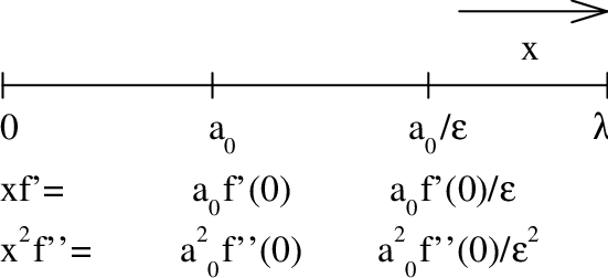
Figure 1: Schematic of domain $0<x<\lambda$, showing origin where there is a typically a stagnation point, and $x=a_{0}\ll a_{0}/\epsilon$, explained in the text. $r_{2}=0.25$.

The simplest example of a function $f$ satisfying $f^{\prime\prime}=\mathcal{O}(\epsilon)f^{\prime}$ (prime denotes spatial derivative) is unfortunate, namely the exponential $\exp(x/\lambda)$, because the rapid growth of the function with distance implies the linear region may be hard to observe in either numerical or laboratory experiments. Nonetheless, there will be other, less rapidly spatially increasing functions, and the linear fields’ model should be valid provided $\|x\|/a_{0}\leq\mathcal{O}(1)$. Evidently the lengthscale $a_{0}$ needs to be smaller than the domain size $\lambda$, and in practice it will be set by the initial ratio of function to first derivative $\|Q^{j}\|/\|Q^{j}_{i}\|$ if $B^{j}\neq 0$.

There remains the question as to whether the ordering remains consistent under time evolution, that is to say whether Eq. (17) implies that second order field derivatives also do not grow. In the case where $U^{i}=0$ contracting $Q^{j}_{kl}$ with $\dot{Q}^{j}_{kl}$ from Eq. (17) gives

$$Q^{j}_{kl}\dot{Q}^{j}_{kl}=Q^{j}_{kl}U^{i}_{l}Q^{j}_{ik}-Q^{j}_{kl}U^{i}_{k}Q^{j}_{il}-Q^{j}_{kl}U^{j}_{i}Q^{i}_{kl}$$ (36)

provided $U^{j}_{ki}=0$ is also assumed. In each of the three terms, the antisymmetric tensor $U$ is contracted with a symmetric tensor consisting of the product of $Q$ with itself, hence each vanishes separately. This statement does not depend on the coordinate system used hence taking $Q=B$, the sum of the squares of the $B^{i}_{jk}$ is shown to be conserved for flows of type Eq. (34) also (the Lie-Taylor series expansion of Subsection 2.1 of Section 2 could have been developed in the coordinates where $V$ was antisymmetric). Given the same result at the end of Subsection 2.1 of Section 2 for first order $Q$ derivatives, it should be evident that a similar analysis could be conducted at any higher order.

3 Case study: Dolzhansky-Kirchhoff Equations

3.1 Derivation

The Kirchhoff equations for incompressible MHD after Dolzhansky [4] follow upon assuming that the transformation of coordinates applied to an antisymmetric matrix representation of the velocity gradient matrix $U$ is a simple anisotropic scaling

$$x_{i}=a_{(i)}x^{i}$$ (37)

so that $\ell_{ij}$ introduced in Subsection 2.3 of Section 2 is diagonal. The convention is adopted that suffices on $x$, as distinct from on fields $u^{i}$ and $\varrho$, denote Cartesian coordinates.

Without the anisotropy induced by this scaling, it helps to note that Dolzhansky has introduced a basis for the fields which takes the form

$${\bf e}_{i}\propto\hat{\bf x}_{i}\times{\bf x}$$ (38)

where $\hat{\bf x}_{1},\hat{\bf x}_{2},\hat{\bf x}_{3}$ are the unit vectors in Cartesian coordinates. Hence for each $i$, ${\bf e}_{i}\cdot{\bf x}=0$ and the linear fields’ flow expressed in terms of this basis, viz.

$${\bf u}({\bf x},t)=\Sigma_{k=1}^{3}\varpi"_{k}{\bf e}_{k},$$ (39)

where the coefficients $\varpi"_{k}$ vary only with time, has streamlines and indeed streaklines which are confined to spherical surfaces. Under the transformation Eq. (37), and indeed any affine scaling, spheres become ellipsoids and the basis becomes non-orthogonal, but the same local confinement property applies. Rather less satisfactorily from the physical point-of-view as mentioned in Subsection 1, although justification was attempted in Subsection 2.4 of Section 2, the magnetic field has to have the same basis and therefore is forced to have this local confinement property, viz.

$${\bf B}({\bf x},t)=\iota"_{k}(t){\bf e}_{k},$$ (40)

The derivation of the Kirchhoff equations from the Lie-Taylor series approach of Section 2 proceeds by introducing the transformed vector $\mbox{\boldmath$\Omega$}=\ell^{-1}\mbox{\boldmath$\omega$}$, in components $\Omega^{i}=\ell_{ji}\omega^{j}$, so that Eq. (11) for $Q^{i}$ as the vorticity (i.e. with $Q^{i}=\omega^{i}$) becomes

$$\dot{\mbox{\boldmath$\Omega$}}=V\mbox{\boldmath$\Omega$}$$ (41)

The Kirchhoff ‘vorticity’ equation is completed when $\Omega_{i}$ is expressed in terms of the entries in $\varpi_{k}$ in $V$. Eq. (31) and Eq. (33) when combined give

$$\Omega^{i}=e_{ijk}G_{kl}V_{lj}=e_{ijk}G_{kl}e_{ljm}\varpi_{m}$$ (42)

which using Einstein’s identity becomes

$$\Omega^{i}=G_{ki}\varpi_{k}-G_{kk}\varpi_{i}$$ (43)

Taking $\ell_{ij}$ or equivalently $G_{ij}$ to be diagonal, Eq. (43) yields the relation

$$\Omega^{i}=I_{(i)}\varpi_{i}/\sqrt{g}$$ (44)

where $I_{i}=g^{\prime}_{ii}$ denotes e.g. that the term $g_{11}$ is omitted from the trace of $g$ in the definition of $\varpi_{1}$, etc.

Analogous to Eq. (33), write

$$K_{qr}=e_{qrk}\iota_{k}$$ (45)

and explicitly writing

$$I_{i}=a_{j}^{2}+a_{k}^{2},\;\;\;(ijk)\mbox{ a permutation of }(123)$$ (46)

the vector vorticity equation becomes

$$\dot{\varpi}_{1} = r_{1}(\varpi_{2}\varpi_{3}-\iota_{2}\iota_{3})$$

$$\dot{\varpi}_{2} = r_{2}(\varpi_{1}\varpi_{3}-\iota_{1}\iota_{3})$$ (47)

$$\dot{\varpi}_{3} = r_{3}(\varpi_{1}\varpi_{2}-\iota_{1}\iota_{2})$$

where

$$r_{1} = (I_{3}-I_{2})/I_{1}=(a^{2}_{2}-a^{2}_{3})/(a^{2}_{2}+a^{2}_{3})$$

$$r_{2} = (I_{1}-I_{3})/I_{2}=(a^{2}_{3}-a^{2}_{1})/(a^{2}_{1}+a^{2}_{3})$$ (48)

$$r_{3} = (I_{2}-I_{1})/I_{3}=(a^{2}_{1}-a^{2}_{2})/(a^{2}_{1}+a^{2}_{2})$$

Note that $|r_{i}|\leq 1$ each $i$, and that the $r_{i}$ are not independent, but related by

$$r_{1}+r_{2}+r_{3}+r_{1}r_{2}r_{3}=0$$ (49)

so that e.g. $r_{3}=-(r_{1}+r_{2})/(1+r_{1}r_{2})$, and the inverse relations are for example

$$\frac{I_{2}}{I_{1}} = \frac{1-r_{1}}{1+r_{2}}$$

$$\frac{I_{3}}{I_{1}} = \frac{1+r_{1}}{1-r_{3}}$$ (50)

$$\frac{I_{3}}{I_{2}} = \frac{1-r_{2}}{1+r_{3}}$$

The vector electric current equation, using Eq. (35) is simply

$$\dot{\iota}_{1} = \varpi_{2}\iota_{3}-\varpi_{3}\iota_{2}$$

$$\dot{\iota}_{2} = \varpi_{3}\iota_{1}-\varpi_{1}\iota_{3}$$ (51)

$$\dot{\iota}_{3} = \varpi_{1}\iota_{2}-\varpi_{2}\iota_{1}$$

Note that, as might have been anticipated, $\varpi"$ and $\varpi$, $\iota"$ and $\iota$ may respectively be identified. Further, although the above approach may seem to enable the generalisation of Dolzhansky’s approach to a non-orthogonal coordinate system, this does not in fact constitute a different physical situation because the affine transformation of an ellipsoid is another ellipsoid.

The Kirchhoff equations have a conserved Hamiltonian

$$H_{0}=I_{1}(\varpi^{2}_{1}+\iota^{2}_{1})+I_{2}(\varpi^{2}_{2}+\iota^{2}_{2})+I_{3}(\varpi^{2}_{3}+\iota^{2}_{3})$$ (52)

together with a cross-helicity

$$H_{1}=I_{1}(\varpi_{1}\iota_{1})+I_{2}(\varpi_{2}\iota_{2})+I_{3}(\varpi_{3}\iota_{3})$$ (53)

and Eq. (3.1) as discussed in Subsection 2.1 of Section 2 has a (Casimir) invariant $C_{0}=\iota^{2}_{1}+\iota^{2}_{2}+\iota^{2}_{3}$. The Kirchhoff equations may be transformed into the equations of motion of a charged particle on a sphere, see [9, § 1], although the transformation is not well explained, and not mentioned in [3]. However, the most efficient way to proceed is to note that the Dolzhansky variant of the Kirchhoff equations is the Clebsch case, see ref [10, § 2.4] and so is completely integrable with $3$ invariants

$$C_{1} = \iota^{2}_{1}+\varpi^{2}_{2}/r_{2}-\varpi^{2}_{3}/r_{3}$$

$$C_{2} = \iota^{2}_{2}-\varpi^{2}_{1}/r_{1}+\varpi^{2}_{3}/r_{3}$$ (54)

$$C_{3} = \iota^{2}_{3}+\varpi^{2}_{1}/r_{1}-\varpi^{2}_{2}/r_{2}$$

In fact there are two remaining degrees of freedom, since $H_{0}=I_{1}C_{1}+I_{2}C_{2}+I_{3}C_{3}$ and $C_{0}=C_{1}+C_{2}+C_{3}$.

3.2 Catastrophic Behaviour

It is of interest for comparison with ideal MHD to understand the transient behaviour of Dolzhansky’s equations. Supposing that the magnetic field has negligible dynamical effect, then it evolves kinematically in a flow, described by vorticity variables which obey Euler’s equations for the motion of a massless spinning top in classical mechanics. For such a body, it is a classical result that if the $I_{i}$, regarded now as moments of inertia of the top, satisfy $I_{3}>I_{1}>I_{2}$ then motion about the $1$-axis is unstable. Thus a significant transient is expected when a slow variation of $a_{i}$ is arranged such that $I_{3}$ approaches then drops below $I_{1}$, so that rotation about the $3$-axis is destabilised.

This transient corresponds to the near disappearance (see Appendix 6(b)) of the effective potential when $r_{2}=0$ so that the system moves ballistically on the timescale of $\omega_{3}\approx 1$ away from a now unstable equilibrium, i.e. the rate at which the instability threshold is crossed is of little importance. This is illustrated in Figure 2, where the initial conditions ensure in fact that $\iota_{i}=0$ for all time.

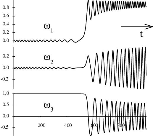
Figure 2: Euler’s equations, initial conditions $\omega_{1}=\omega_{2}=0.01$, $\omega_{3}=1$ $I_{1}=2.25$, $I_{2}=1.25$, $I_{3}(0)=2.5$, slowly varying $I_{3}$ satisfies $I_{3}=I_{3}(0)-0.001t/2$.

This behaviour may also be deduced from the properties of Jacobi elliptic functions under parameter variation.

Energy remains bounded in the case of top dynamics because the system ends in a different well with different rotation and translation direction. The implications for field kinematics is the possibility of a sudden transient which redirects not only the vortex but also the electric current direction. This is reminiscent of the ideal MHD kink where components of field and current in new directions appear. It has however to be established that this behaviour extends to the case of a dynamically active magnetic field.

Figures 3– 4 support this contention. All the field components now have initial conditions $0.01$, except $\omega_{3}=0.1$ and $\iota_{3}=1$, so that this is a study of the full Dolzhansky equations where the magnetic field is dominant. Figure 3 exhibits a similar transient to the ‘spinning top’ or field-free case when the stability boundary $r_{1}=0$ (see Appendix 6(a)) is again crossed at the rate $0.001$. The exact nature of this transient requires further examination, but it will be seen from Figure 4 that the timescale for say $\iota_{3}$ to reverse changes only by a factor of three (from approximately $40$ to $110$) when the crossing rate drops by a factor of $100$.

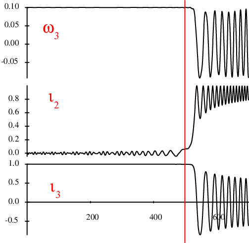
Figure 3: Dolzhansky-Kirchhoff equations with slowly varying $r_{1}=-0.5+0.001t$, $r_{2}=0.25$.

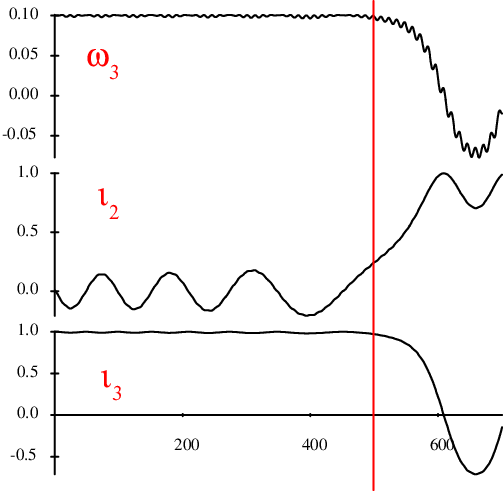
Figure 4: Dolzhansky-Kirchhoff equations with very slowly varying $r_{1}=-0.005+0.000\,01t$, $r_{2}=0.25$.

3.3 Lie Algebra

The scaling Eq. (37) applied to the basis functions Eq. (38) leads to Dolzhansky’s basis functions ${\bf e}_{i}$ (${\bf W}_{i}$ in the notation of ref [4])

$${\bf e}_{i}=-\frac{a_{j}}{a_{k}}x_{k}\hat{\bf x}_{j}+\frac{a_{k}}{a_{j}}x_{j}\hat{\bf x}_{k},\;\;\;(ijk)\mbox{ a permutation of }(123)$$ (55)

where $\hat{\bf x}_{j}$ are the usual Cartesian basis vectors, and the summation convention is not employed. These vectors are solenoidal $\nabla.{\bf e}_{i}=0$, hence the Lie derivative of one basis vector with another may be efficiently evaluated as

$$[{\bf e}_{i},{\bf e}_{j}]=\nabla\times({\bf e}_{i}\times{\bf e}_{j})$$ (56)

Direct substitution of Eq. (55), shows that

$$[{\bf e}_{i},{\bf e}_{j}]={\bf e}_{k},\;\;\;(ijk)\mbox{ even permutation of }(123)$$ (57)

This is a particularly simple definition of a Lie algebra, since in general the Lie bracket is allowed to be an arbitrary linear combination of the basis vectors with coefficients known as structure constants. The importance of Eq. (57) is that the current evolution equations Eq. (3.1) follow immediately from the corresponding PDE, Eq. (1). However, the vorticity evolution equation involves the Lie bracket of ${\bf e}_{i}$ and its curl.

The latter quantity is

$$\nabla\times{\bf e}_{i}=(\frac{a_{j}}{a_{k}}+\frac{a_{k}}{a_{j}})\hat{\bf x}_{i},\;\;\;(ijk)\mbox{ a permutation of }(123)$$ (58)

Choosing ${\bf c}_{i}=a_{(i)}\hat{\bf x}_{i}$, $\nabla\times{\bf e}_{i}=I_{(i)}{\bf c}_{i}/\sqrt{g}$ and

$$[{\bf e}_{i},{\bf c}_{j}]={\bf c}_{k},\;\;\;(ijk)\mbox{ even permutation of }(123)$$ (59)

and obviously $[{\bf c}_{i},{\bf c}_{j}]={\bf 0}$. Given these new Lie brackets, the ODE, Eq. (3.1), may be written down immediately from the PDE, Eq. (2).

4 Resistivity

Resistivity, either in the classical isotropic case, or possibly as the result of a renormalisation approach to turbulence, leads to an additional term in the induction equation, which assuming $\rho=\mbox{const.}$, becomes

$$\frac{\partial{\bf B}}{\partial t}=[{\bf u},{\bf B}]+\nabla\times\eta\nabla\times{\bf B},$$ (60)

If ${\bf B}$ has a linear field representation in Cartesian coordinates, then $\nabla\times\eta\nabla\times{\bf B}=\nabla\eta\times\nabla\times{\bf B}$. Considering first the spherical, or unscaled case as discussed at the start of Subsection 3.1 of Section 3, the resistive term contains contributions of the form $\nabla\eta\times\hat{\bf x}_{i}$. These new terms are simply expressible in Dolzhansky’s basis ${\bf e}_{i}$ if $\nabla\eta\propto{\bf x}$. It is then plausible, as may be verified by direct substitution, that in scaled coordinates, if the resistivity is written

$$\eta=\eta_{0}+\bm{\eta}_{1}\cdot{\bf x}+\eta_{2}\left(\frac{x^{2}_{1}}{a^{2}_{1}}+\frac{x^{2}_{2}}{a^{2}_{2}}+\frac{x^{2}_{3}}{a^{2}_{3}}\right)$$ (61)

then this simple relationship still applies ($\eta_{0}$ and $\eta_{1}$ do not directly affect the model evolution of linear field ${\bf B}$).

It follows that for quadratic spatial dependence of resistivity of the form Eq. (61), the equations for electric current variation acquire terms

$$\eta_{2}\left(\frac{1}{a_{j}^{2}}+\frac{1}{a_{k}^{2}}\right)\iota_{i},\;\;\;(ijk)\mbox{ permutation of }(123)$$ (62)

and become

$$\dot{\iota}_{1} = \varpi_{2}\iota_{3}-\varpi_{3}\iota_{2}+\eta_{2}\left(\frac{1}{a_{2}^{2}}+\frac{1}{a_{3}^{2}}\right)\iota_{1}$$

$$\dot{\iota}_{2} = \varpi_{3}\iota_{1}-\varpi_{1}\iota_{3}+\eta_{2}\left(\frac{1}{a_{1}^{2}}+\frac{1}{a_{3}^{2}}\right)\iota_{2}$$ (63)

$$\dot{\iota}_{3} = \varpi_{1}\iota_{2}-\varpi_{2}\iota_{1}+\eta_{2}\left(\frac{1}{a_{1}^{2}}+\frac{1}{a_{2}^{2}}\right)\iota_{3}$$

Note that $\eta$ must be maximal at the origin ($\eta_{2}<0$) otherwise the new resistivity terms imply exponential growth of the square current $(\iota^{2}_{1}+\iota^{2}_{2}+\iota^{2}_{3})$. Although this conclusion seems rather strange, it is in fact consistent with the conclusion drawn by Forbes at al [11], who find that only for locally maximum resistivity is the Petschek mechanism for reconnection structurally stable.

5 Conclusion

This work has reinforced the contentions of ref [4] that the Dolzhansky-Kirchhoff (D-K) equations exhibit mathematical properties important for understanding nonlinear magnetohydrodynamics (MHD) in the limit of small or vanishing resistivity. Section 2 illustrates the general mathematical framework into which the equations fit, then Subsection 3.1 of Section 3 shows how the D-K equations emerge when a solution for ideal MHD is sought as a Taylor series in Cartesian coordinates. Subsection 3.2 of Section 3 shows that catastrophism is natural in the system, in a consistent sense, namely that model variables remain bounded, despite the dynamic timescale.

The derivation of the model also illustrates important features of the Lie derivative, specifically its anti- or skew-symmetric nature as demonstrated by its replacement by the matrix-commutator in Section 2. In Section 2 also, important conservation relations, extending to arbitrary order of power of the unknowns, are illustrated. Continuing the mathematical note, Subsection 3.3 of Section 3 shows the importance of the concept of Lie algebra when seeking time-dependent solutions of nonlinear MHD. All these properties imply that the D-K equations should also be an aid to understanding the reduction of PDEs to non-canonical Hamiltonian systems and subsequent analysis [12, 3].

As already incidentally demonstrated by the catastrophic simulations, the sixth order D-K equations, with four invariants, are capable of exhibiting oscillation with two different timescales and amplitudes over a wide range of frequencies. The reduction of nonlinear MHD to a low order Hamiltonian system highlights the likely prevalence of oscillation in ideal MHD, since such Hamiltonian systems do not generically possess attracting steady solutions and their stability can only be established in a Lyapunov sense. It is plausible that these considerations extend to the case of small resistivity when current sheets do not form.

Other important physical behaviour, such as the existence and behaviour of nonlinear Alfvenic solutions, corresponding to $\iota_{k}=c_{(k)}\varpi_{k}$, for some constants $c_{k}$, may be deduced from known results for the Kirchhoff equations [10].

Section 4 shows how resistivity may be included in the model so that the physics of reconnection, believed important in many laboratory and astrophysical contexts, may be studied. In the context of laboratory plasmas, specifically the central region of tokamaks, the structural stability question raised by Forbes et al requires further analysis.

Dolzhansky [4] describes how other important physics such as rotation and gravity (with buoyancy force thanks to a density evolving due to a thermal evolution equation), may be included. Another application of linear fields, which will require development of the Lie-Taylor expansion for the momentum conservation equation along the lines of the mass conservation equation in Subsection 2.2 of Section 2, is to partially ionised plasma where mass and momentum sources allow outflow boundary conditions, e.g. in 1-D models of the tokamak edge.

Further mathematical and physical insights into these more complicated inviscid or almost-inviscid situations may be anticipated. As touched upon in ref [7], the vorticity evolution equation presents the problem that the algebra must involve not only basis functions but their curls. Progress may be made using Beltrami or ‘screw’ fields since these offer the potential to explore nonorthogonal geometries without the explicit appearance of the metric tensor, but this will be discussed elsewhere.

I have no competing interests. The ODE integrations were performed using Hindmarsh’s LSODE package. This work has been funded by the RCUK Energy Programme [grant number EP/I501045]. To obtain further information on the data and models underlying this paper please contact PublicationsManager@ccfe.ac.uk.

6 Appendices

6.1 Stability Analysis

Note that $\omega$ is used as a synonym for $\varpi$ in the following.

6.1.1 Aligned Vorticity and Current

Without loss of generality, assume that the vorticity and current are aligned in the direction of the $3$-axis, with $\omega_{3}=W$ and $\iota_{3}=J$ and all other components of $\mathcal{O}(\epsilon)$ at time $t=0$. With these assumptions Eq. (3.1) and Eq. (3.1) become respectively

$$\dot{\omega}_{1} = r_{1}(W\omega_{2}-J\iota_{2})$$ (64)

$$\dot{\omega}_{2} = r_{2}(W\omega_{1}-J\iota_{1})$$ (65)

$$\dot{\omega}_{3} = \mathcal{O}(\epsilon^{2})$$

$$\dot{\iota}_{1} = J\omega_{2}-W\iota_{2}$$ (66)

$$\dot{\iota}_{2} = W\iota_{1}-J\omega_{1}$$ (67)

$$\dot{\iota}_{3} = \mathcal{O}(\epsilon^{2})$$

Differentiating Eq. (65) with respect to time, and substituting for first derivatives using Eq. (64) and Eq. (66) gives

$$\ddot{\omega}_{2}=r_{2}\omega_{2}(r_{1}W^{2}-J^{2})+r_{2}JW(1-r_{1})\iota_{2}$$ (68)

Similarly differentiating Eq. (67) with respect to time, and substituting for first derivatives using Eq. (64) and Eq. (66) gives

$$\ddot{\iota}_{2}=(r_{1}J^{2}-W^{2})\iota_{2}+JW(1-r_{1})\omega_{2}$$ (69)

Seeking solutions varying in time $\propto\exp(st)$ to Eqs (68) and (69) gives the determinantal equation $\det(M)=0$ where

$$M=\begin{pmatrix}-s^{2}+m_{11}&m_{12}\\ r_{2}m_{12}&-s^{2}+m_{22}\end{pmatrix}$$ (70)

with $m_{11}=r_{1}J^{2}-W^{2}$, $m_{12}=JW(1-r_{1})$ and $m_{22}=r_{2}(r_{1}W^{2}-J^{2})$. The resulting stability polynomial is

$$s^{4}-\left(J^{2}(r_{1}-r_{2})+W^{2}(r_{1}r_{2}-1)\right)s^{2}-r_{1}(J^{2}-W^{2})^{2}=0$$ (71)

Instability may be avoided if both roots of the corresponding quadratic (with $x=s^{2}$) are negative, implying $\beta<0$ and $r_{1}<0$, where $\beta$ is the coefficient of $s^{2}$. The former means

$$r_{2}>\frac{(r_{1}J^{2}-W^{2})}{(J^{2}-r_{1}W^{2})}$$ (72)

Note that this stability analysis may be checked by differentiating Eqs (64) and (66) with respect to time and substituting using Eqs (65) and (67). Numerical solution in the text confirms that $r_{1}=0$ is indeed a stability boundary.

6.1.2 Orthogonal Vorticity and Current

Without loss of generality, assume that the vorticity and current are aligned in the directions of the $3$-axis and the $1$-axis respectively, with $\omega_{3}=X$ and $\iota_{1}=K$ and all other components of $\mathcal{O}(\epsilon)$ at time $t=0$. With these assumptions Eq. (3.1) and Eq. (3.1) become respectively

$$\dot{\omega}_{1} = r_{1}X\omega_{2}$$ (73)

$$\dot{\omega}_{2} = r_{2}(X\omega_{1}-K\iota_{3})$$ (74)

$$\dot{\omega}_{3} = -r_{3}K\iota_{2}$$

$$\dot{\iota}_{1} = -X\iota_{2}$$ (75)

$$\dot{\iota}_{2} = \iota_{1}\omega_{3}=XK$$ (76)

$$\dot{\iota}_{3} = -K\omega_{2}$$

Eq. (76) shows that $\iota_{2}$ grows on a $\mathcal{O}(1)$ timescale unless either $X=o(1)$ or $K=o(1)$.

In the former case $X=o(1)$, differentiating Eq. (74) gives

$$\ddot{\omega}_{2}=r_{2}K^{2}\omega_{2}$$ (77)

so there might be stability if $r_{2}<0$, but even so $\omega_{3}$ varies in time proportional to $\iota_{2}$. Similarly in the latter case $K=o(1)$

$$\ddot{\omega}_{2}=r_{1}r_{2}X^{2}\omega_{2}$$ (78)

and there is again an apparently secular variation, this time in $\iota_{1}$.

Thus it seems that there is no stable steady solution with orthogonal vorticity and current. This conclusion is supported by analysis with $K,\;X=\mathcal{O}(1)$ that follows if Eq. (76) is differentiated with respect to time without assuming that $\omega_{3}$ and $\iota_{1}$ are constant. For then

$$\ddot{\omega}_{3}=-r_{3}K^{2}\omega_{3}$$ (79)

implying that $\omega_{3}$ oscillates with frequency $\sqrt{r_{3}}K$ (provided $r_{3}>0$). It also follows that $\iota_{1}$ and $\iota_{2}$ oscillate with frequencies $X$ and $\sqrt{(X^{2}+r_{3}K^{2})}$ respectively provided the $\omega_{3}$ oscillation is slow.

For the $\omega_{1}$ and $\iota_{3}$ dynamic, there is a determinantal equation $\det(M^{\prime})=0$ where

$$M^{\prime}=\begin{pmatrix}-s^{2}+m^{\prime}_{11}&r_{1}m^{\prime}_{12}\\ m^{\prime}_{12}&-s^{2}+m^{\prime}_{22}\end{pmatrix}$$ (80)

with $m^{\prime}_{11}=r_{1}r_{2}X^{2}$, $m^{\prime}_{12}=r_{2}KX$ and $m^{\prime}_{22}=r_{2}K^{2}$. This leads to a quadratic in $x=s^{2}$ with roots $x=0$ and

$$x=r_{2}(K^{2}+r_{1}X^{2})$$ (81)

This may imply instability unless $r_{2}<0$ and $r_{1}<-K^{2}/X^{2}$ or $r_{2}>0$ and $r_{1}>-K^{2}/X^{2}$.

6.2 ‘Disappearance’ of the Potential

The surprising, at first hearing, remark that the potential almost disappears when $I_{3}=I_{1}$, is explained if each component of vorticity is treated as evolving in its own separate potential. The relevant equations may be derived by differentiating each of the equations for $\varpi_{i}=\omega_{i}$ in Eq. (3.1) separately with respect to time, then eliminating first derivatives in terms of the $\omega_{i}$. This gives equations specifiable, given

$$\ddot{\omega}_{3}=r_{3}\omega_{3}(r_{1}\omega_{2}^{2}+r_{2}\omega_{1}^{2}),$$ (82)

as even cyclic permutations of the equation’s suffices $(123)$. Substituting for $C_{1},\;C_{2},\;C_{3}$ in Eq. (82) and permutations then gives

$$\ddot{\omega}_{1} = r_{2}r_{3}\omega_{1}\left((C_{2}-C_{3})r_{1}+2\omega_{1}^{2}\right)$$

$$\ddot{\omega}_{2} = r_{1}r_{3}\omega_{2}\left((C_{3}-C_{1})r_{2}+2\omega_{2}^{2}\right)$$ (83)

$$\ddot{\omega}_{3} = r_{1}r_{2}\omega_{3}\left((C_{1}-C_{2})r_{3}+2\omega_{3}^{2}\right)$$

Each equation Eq. (83) represents the motion of a particle in a potential $V_{i}$, e.g. given by

$$2V_{3}(\omega_{3})=r_{1}r_{2}(C_{1}-C_{2})r_{3}\omega^{2}_{3}+r_{1}r_{2}\omega^{4}_{3}$$ (84)

in the case of $\omega_{3}$, and obvious permutations for the other $\omega_{i}$. When $I_{3}=I_{1}$, $r_{2}=0$ from Eq. (3.1), and it follows that the quadratic potential contributions to $V_{i}$ vanish for each $i$, and only the quartic term in $V_{2}$ survives. The corresponding variable is $\omega_{2}$ which is small at least initially, hence the particle representing vector $\omega$ is able to move ballistically, as though there were no potential forces present.

The table gives values to $2$ decimal places for the coefficients of $2V_{i}$ at the start of the simulation shown in Figure 2, all of which change sign at $r_{2}=0$ except the one marked with a dagger. The corresponding dependence of the potential $V_{i}$ on $\omega_{i}$ is denoted by ‘U’,‘W’ or ‘M’, with the letter corresponding to the approximate shape of the potential. Thus $\omega_{3}$ sits stably in the well at the bottom of the right-hand of the ‘W’ potential, which flips to become an ’M’ shape in $r_{2}>0$ whereupon $\omega_{3}$ oscillates in the well in the centre of the ‘M’.

Table 1: Coefficients of effective potentials for Euler’s equations at start of simulation.

Term	$2V_{1}$	$2V_{2}$	$2V_{3}$
$\omega^{2}$	$-0.11$	$-0.12$	$0.24$
$\omega^{4}$	$0.08$	$-0.24$†	$-0.12$
$r_{2}<0\mapsto>0$	$M\mapsto W$	$U\mapsto W$	$W\mapsto M$
	†does not change sign.

References

- [1] W. Arter. Potential Vorticity Formulation of Compressible Magnetohydrodynamics. Physical Review Letters, 110(1):015004, 2013. DOI:10.1103/PhysRevLett.110.015004.
- [2] J.W. Dungey. Cosmic Electrodynamics. CUP, 1958.
- [3] V.I. Arnol’d and B.A. Khesin. Topological methods in hydrodynamics. Springer, 1998.
- [4] F.V. Dolzhansky. On the mechanical prototypes of fundamental hydrodynamic invariants and slow manifolds. Physics-Uspekhi, 48:1205, 2005.
- [5] H. Lamb. Hydrodynamics. CUP, 1997.
- [6] W. Arter. Local models of magnetohydrodynamics. Physics Letters, 122A:253–256, 1987.
- [7] W. Arter. Geometric Results for Compressible Magnetohydrodynamics. arXiv preprint arXiv:1309.7172, 2013.
- [8] V.S. Imshennik and S.I. Syrovatskii. Two-dimensional flow of an ideally conducting gas in the vicinity of the zero line of a magnetic field. Sov. Phys.–JETP, 25(4):656–664, 1967.
- [9] V.I. Arnold and S.P. Novikov. Dynamical systems IV: Symplectic geometry and its Applications, 2nd Ed. Springer, 1990.
- [10] P. Holmes, J. Jenkins, and N.E. Leonard. Dynamics of the Kirchhoff equations I: Coincident centers of gravity and buoyancy. Physica D: Nonlinear Phenomena, 118(3-4):311–342, 1998.
- [11] T.G. Forbes, E.R. Priest, D.B. Seaton, and Y.E. Litvinenko. Indeterminacy and instability in Petschek reconnection. Physics of Plasmas, 20(5):052902, 2013.
- [12] D.D. Holm, J.E. Marsden, and T.S. Ratiu. The Euler Poincare Equations and Semidirect Products with Applications to Continuum Theories. Advances in Mathematics, 137:1–81, 1998.