Bayesian Analysis of Immune Response Dynamics
with Sparse Time Series Data

Abstract

In vaccine development, the temporal profiles of relative abundance of subtypes of immune cells (T-cells) is key to understanding vaccine efficacy. Complex and expensive experimental studies generate very sparse time series data on this immune response. Fitting multi-parameter dynamic models of the immune response dynamics– central to evaluating mechanisms underlying vaccine efficacy– is challenged by data sparsity. The research reported here addresses this challenge. For HIV/SIV vaccine studies in macaques, we: (a) introduce novel dynamic models of progression of cellular populations over time with relevant, time-delayed components reflecting the vaccine response; (b) define an effective Bayesian model fitting strategy that couples Markov chain Monte Carlo (MCMC) with Approximate Bayesian Computation (ABC)– building on the complementary strengths of the two approaches, neither of which is effective alone; (c) explore questions of information content in the sparse time series for each of the model parameters, linking into experimental design and model simplification for future experiments; and (d) develop, apply and compare the analysis with samples from a recent HIV/SIV experiment, with novel insights and conclusions about the progressive response to the vaccine, and how this varies across subjects.

AMS subject classifications: 62P10, 62M99

Keywords and Phrases: Approximate Bayesian Computation (ABC); Bayesian Inference; Dynamic Models; Immunology; Learnability of Parameters; Markov chain Monte Carlo (MCMC); ODE Models; Sparse Data; Time Delays; Vaccine Design

1 Introduction

In vaccine design and development, experiments in non-human primates (NHPs) are necessary preludes to human clinical trials. Our focus here is on a key case in point, that of new HIV/SIV immunization strategies. While becoming more prevalent, NHP vaccination experiments are expensive and complex, so typically generate small sample sizes and a limited number of longitudinal observations [9, 14, 11]. Mathematical modeling of the immune response dynamics to vaccination can provide insight into the mechanisms underlying vaccine efficacy and help predict the likely human response to the immunization strategy [8, 27, 5, 20]. To capture the complexity of the immune response, such mathematical models are often represented using coupled systems of nonlinear ordinary differential equations (ODEs). We are then faced with the challenges of model fitting with multiple model parameters on very sparse data. There is also a key interest in variability in these characterizing parameters across subjects, since NHPs come from outbred populations so that the immune response is likely to vary across individuals.

We address these general questions in a specific vaccine design study, involving evaluation of efficacy of a replicating Adenovirus Simian Immunodeficiency Virus (SIV) vector [17] introduced via different mucosal routes in a collection of macaques [16]. We summarize the context and experiment, and address questions of dynamic modeling of the vaccine response of each macaque. Beginning with coupled systems of ODEs for the vaccine response, we discretize to define a class of non-linear, discrete-time state-space models for the data defined by cell subtype frequencies. This model framework builds on prior models in the field, while going much further with innovations in time-delay modeling and discretization. We also describe a mapping of model parameters to dimensionless parameters for fundamental characterization and comparison across subjects.

Standard computational methods for model fitting– analytic approximations coupled with either Markov chain Monte Carlo [15, 25], or sequential Monte Carlo including Approximate Bayesian Computation (ABC) [e.g., 13, 21, 18, 2]– are fundamentally challenged due to non-linearities and data sparsity. After exploring such approaches, we have defined with a creative coupling of MCMC and ABC methods that builds on the complementary strengths of the two approaches.

In any modeling context where data is very sparse, questions should arise about which of the parameters are informed upon, at all, and the extent of the information content of the data for each parameter. We discuss and investigate this here, evaluating the prior-to-posterior mapping via entropy and variance to quantify “learnability” of parameters from the sparse time series data. This is useful in interpreting posterior summaries and comparing across experimental subjects, and aids thinking about potential model simplifications and design for future experiments.

Application to the macaque data is discussed and evaluated in the context of the goals of the experiment. The precision of inferences on temporal profiles in the immune response is highlighted along with these questions of model specification and potential parameter redundancy. We see real differences between some of the response-characterizing parameters across individuals, and strong evidence from the overall study that there is a significant time delay in memory T-cells responding to the vaccine interventions. These broad summaries alone represent novel and meaningful findings in the HIV/SIV vaccine response field. Moreover, the analyses suggest that the dynamics of the immune response depends on the vaccination route,(i.e., the way in which the individual is vaccinated). This is a result that is not obvious from inspection of the time series data alone, and is a novel and potential important finding in its own right, suggesting the need– and likely design principles– for further experiments.

2 Basics of Vaccine Biology and Experiment

We performed a longitudinal study to compare the mucosal immune response when a prime-boost vaccine using replication-competent viral vector was given via different routes. Replication-competent Adenovirus (Ad5) with recombinant Simian Immunodeficiency Virus (SIV) Gag genes (Ad5hr-SIVgag) and a GFP marker for tracking was administered to Indian Rhesus macaques via intra-nasal/intra-tracheal, intra-vaginal and intra-rectal routes. The macaques were vaccinated twice with the replicating Ad recombinants (encoding SIV env/rev and gag, plus Ad-GFP) at weeks 0 and 12, and boosted with SIV envelope protein plus adjuvant at weeks 24 and 36 of the study. Relative abundance of functionally and maturationaly different T-cell subtypes were estimated from flow cytometric assays [e.g., 3, 4, 12] on samples from gut mucosa and peripheral blood. A small number of the macaques also had 2-4 measurments of GFP-labelled Adnovirus infected macrophages in the gut mucosa. The summary estimates of cell subtype proportions at each time point assayed provide the raw time series for each subject macaque. The key cellular subtype of interest here is the antigen-specific memory T-cells, and models will address its relation to the level of abundance of the adenovirus-infected macrophages over time.

Replication-competent vectors continue to propagate themselves after vaccination and can sustain a long-term immune response against the SIV genes encoded by the vector. Hence, we expect that the population size of the antigen-specific memory T-cell population is driven by the size of the replicating vector population. Laboratory experiments suggested that the Adenovirus vector resided in host macrophages in the gut mucosa. Our development of nonlinear models of the dynamics of the Ad5-infected macrophage cells (using GFP-expression as a marker for Ad5 infection) in the rectal mucosa, coupled with the antigen-specific memory T-cell response in the blood, aim at evaluating the effects of different vaccination routes on the host response to a replication-competent Ad5 vector.

3 Conceptual/Qualitative Dynamic Modeling Framework

We begin with stylized thinking in terms of coupled ordinary differential equations (ODEs) to describe the qualitative temporal changes in antigen and cellular concentrations in the immune system [e.g., 6]. This is then extended in practicable statistical model development that involves discrete-time representations of the conceptual differential equations systems, and time-delays in the immune response to vaccine intervention. The discretized system of model equations is overlaid with stochastic components to realistically reflect measurement error and unmodeled structure. The model includes noise and mechanistic rate parameters, initial conditions, and– critically– missing (latent) elements of the data time series on subsets of cell frequencies.

3.1 Basic ODE Model

The motivating ODE model describes evolution in continuous time $t$ of Adenovirus ($V_{t}$) and T-cell memory ($M_{t}$) populations, following immunization of a subject with the adenovirus Ad5hr-SIVgag. With subject-specific parameters, take

$$\begin{array}[]{lcl}{\displaystyle\frac{dV_{t}}{dt}}&=&\beta V_{t}\left(1-{\displaystyle\frac{V_{t}}{K_{V}}}\right),\vspace{0.35cm}\\ {\displaystyle\frac{dM_{t}}{dt}}&=&\alpha V_{t}+\rho V_{t}M_{t}\left(1-{\displaystyle\frac{M_{t}}{K_{M}}}\right).\end{array}$$ (1)

The viral population is described by the first equation, a logistic growth form. In the second equation, the first term has $\alpha=\phi N$ where $N$ represents naïve T-cells; the rate of generation of new naïve cells that recognize viral epitopes in the presence of a persistent Ad5 infection is fixed at $\alpha=\phi N$, and the virus drives their differentiation into into memory cells. The second term reflects density-dependent proliferation of pre-existing memory cells. Finally, $V_{t}$ and $M_{t}$ have natural carrying capacities $K_{V}$ and $K_{M}$, respectively.

3.2 Non-dimensionalization

The essential structure of the model, and a reduced number of parameters, arises via a map to the non-dimensional version of the model. As will be seen later, this has a critical practical role in quantifying learnability of model parameters. Let $\mu$, $\nu$ and $\lambda$ be scaling variables– positive, but otherwise arbitrary and to be chosen– that define

$$v_{t}=V_{t}/\mu,\quad m_{t}=M_{t}/\nu\quad\textrm{and}\quad s=t/\lambda.$$

Then, via the chain rule,

$$\frac{dv_{s}}{ds}=\frac{\lambda}{\mu}\frac{dV_{t}}{dt}\quad\textrm{and}\quad\frac{dm_{s}}{ds}=\frac{\lambda}{\nu}\frac{dM_{t}}{dt}.$$

Substituting in equation (1) gives, after some algebra,

$$\frac{dv_{s}}{ds} =\lambda\beta v_{s}\left(1-\frac{v_{s}}{K_{V}/\mu}\right),$$

$$\frac{dm_{s}}{ds} =\frac{\lambda\alpha\mu}{\nu}v_{s}+\lambda\rho\mu v_{s}m_{s}\left(1-\frac{m_{s}}{K_{M}/\nu}\right).$$

Now choose to set $\mu=K_{V}$, $\nu=K_{M}$ and $\lambda=1/\beta$, so that equation (1) maps to the dimensionless model

$$\begin{array}[]{lcl}{\displaystyle\frac{dv_{s}}{ds}}&=&v_{s}(1-v_{s}),\vspace{0.35cm}\\ {\displaystyle\frac{dm_{s}}{ds}}&=&\eta v_{s}+\psi v_{s}m_{s}(1-m_{s})\end{array}$$ (2)

with $\eta=\lambda\alpha\mu/\nu$ and $\psi=\lambda\rho\mu.$ These dimensionless parameters $(\eta,\psi)$ characterize the model; they aid in exploring essential questions of information content of observed data, and in comparisons across subjects in our later analyses.

4 Initial Discrete-time Stochastic Model

We have sparse observations on $V_{t},M_{t}$ at a small number of time points, and of course these are subject to measurement errors, the nature of these errors being partly quantified in the flow cytometry assays. There is also a need for stochastic elements in the time evolution of $V_{t},M_{t}$ to account for model misspecification, i.e., structure not captured by the model. We now move to the practicable discretized form of the ODE conceptual model and overlay these extensions.

Let $\mathbf{x}_{t}=(V_{t},M_{t})^{\prime}$ be the latent state vector of virus and memory frequencies representing the true underlying population densities for one individual at time $t$. We use reparametrizations $\delta=\beta/K_{V}$ and $\gamma=\rho/K_{M}$ to replace $K_{V},K_{M}$ by new rate constants $\delta,\gamma.$ Note from equation (1) that this yields linear forms in $\beta,\delta,\alpha,\rho,\gamma$ and this simplifies analysis; we can then recover $K_{V}=\beta/\delta,K_{M}=\gamma/\rho$ as desired.

Discretize to time scale $t=h,2h,\ldots,T$ with increment $h>0,$ and suppose observations are made only at times $t_{1}<t_{2}<\cdots<t_{n}.$ Directly via Euler discretization of equation (1), and allowing for measurement errors and state evolution noise, we have

$$\begin{array}[]{lcl}V_{t}=V_{t-h}+h(\beta-\delta V_{t-h})V_{t-h}+\omega_{Vht}\vspace{0.3cm}\\ M_{t}=M_{t-h}+h\alpha V_{t-h}+h(\rho V_{t-h}-\gamma V_{t-h}M_{t-h})M_{t-h}+\omega_{Mht}\end{array}$$ (3)

over all $t=h,\ldots,T.$ The evolution noise $\mbox{\boldmath$\omega$}_{ht}=(\omega_{Vht},\omega_{Mht})^{\prime}$ represents stochastic noise in the state evolution as well as the model misfit. We take this as zero-mean Gaussian with diagonal variance matrix having variances $(\kappa^{2}_{V},\kappa^{2}_{M})$ that are now additional parameters.

Measurements are made at a set of times $t_{1},\ldots,t_{n}.$ So we observe

$$\mathbf{y}_{j}=\mathbf{x}_{t_{j}}+\mbox{\boldmath$\nu$}_{j},\qquad j=1,\ldots,n,$$ (4)

where measurement errors $\mbox{\boldmath$\nu$}_{j}$ are zero-mean Gaussian with diagonal variance matrix having entries $(\sigma^{2}_{V},\sigma^{2}_{M}),$ additional parameters subject to prior information from flow cytometry assays. Sometimes only one of $V_{t},M_{t}$ is measured at a particular $t_{j}$. Let $t\in O_{V}$ and $t\in O_{M}$ be times measurements are made on $V_{t},M_{t}$, respectively. The time sets may or may not intersect. Theoretically, we can reflect this using measurement error variances $(\sigma^{2}_{V}/c_{Vt},\sigma^{2}_{M}/c_{Mt}),$ where $c_{Vt}=1$ but $c_{Mt}\to 0$ when $t\in O_{V}$ but $t\notin O_{M},$ and so forth. This results in minor technical changes to the analysis below.

4.1 Extended Model: Incorporating Time Delays

The initial model form turns out to be unable to reflect a key feature of the data that relates to what in retrospect is anticipated additional complexity in the immune response– that of time delays in the driving of cellular differentiation following vaccine introduction. This is reflected in delay before appearance of Ad5-infected macrophages in the gut mucosa. The basic model above is therefore extended to allow for subject-specific time delays in the effects of the viral population level on the memory cells. Specifically, equation (3) is extended to

$$\begin{array}[]{lcl}V_{t}&=&\begin{cases}V_{t-h}+\omega_{Vht},&\text{if $t\leq\tau_{V}$},\\ V_{t-h}+h\partial\!V_{t-h}+\omega_{Vht},&\text{otherwise;}\end{cases}\vspace{0.1cm}\\ M_{t}&=&\begin{cases}M_{t-h}+\omega_{Mht},&\text{if $t\leq\tau_{V}+\tau_{M}$,}\\ M_{t-h}+h\partial\!M_{t-h}+\omega_{Mht},\phantom{........}&\text{otherwise.}\end{cases}\end{array}$$ (5)

where

$$\begin{array}[]{lcl}\partial\!V_{t-h}&=&(\beta-\delta V_{t-h})V_{t-h},\\ \partial\!M_{t-h}&=&\alpha V_{t-h}+(\rho V_{t-h}-\gamma V_{t-h}M_{t-h})M_{t-h}.\end{array}$$

Here $\tau_{V}$ is the time delay on the direct impact of vaccination on $V_{t},$ and $\tau_{M}$ is the additional delay before $V_{t}$ impacts on memory cells. The parameters are now

$$\Theta=\{\beta,\delta,\alpha,\rho,\gamma,V_{0},\tau_{V},\tau_{M},\sigma^{2}_{V},\sigma^{2}_{M},\kappa^{2}_{V},\kappa^{2}_{M}\}$$ (6)

including the unknown, initial viral level $V_{0}$, all noise, rate and delay parameters. We also note the implied parameters of the dimensionless model are just $\lambda_{V}=\beta\tau_{V}$ and $\lambda_{M}=\beta\tau_{M}.$

5 Bayesian Computation for Model Fitting

With observed data $\mathbf{Y}=\{\mathbf{y}_{t_{j}},\ j=1,\ldots n\},$ we aim to explore the posterior $p(\Theta,\mathbf{X}|\mathbf{Y})$ where $\mathbf{X}=\{\mathbf{x}_{t},\ t=h,2h,\ldots,T\}$ is the trajectory of latent states $V_{t},M_{t}$ over the time period. The model is a complicated, non-linear dynamic model and standard computational methods of MCMC and sequential Monte Carlo, including ABC, are notoriously challenged by the needs to define relevant proposal mechanisms, and high rejection rates associated with long series of latent states. Recent approaches representing current research frontiers focus heavily on biological systems applications [e.g., 15, 2, 7, 10, 26]. The sparsity of data in our studies exacerbates the difficulties. MCMC is challenged by the nonlinearities and truncation to positive states in the model. ABC methods are challenged by the high-dimensionality of the latent states and the interest in relatively diffuse priors for model parameters, so that it is difficult to generate prior:model simulations in the region of the sparse observed data. After detailed experimentation with these and other approaches, including other sequential methods, we have identified a strategy of coupling MCMC with adaptive ABC that draws on their complementary strengths. The two stages are:

• Use MCMC coupled with traditional analytic approximation (local linearization) of the model to define an approximate posterior sample. Knowing that this will be biased in ways that are difficult to assess,

• Use this MCMC sample to define a proposal distribution for an efficient, adaptive ABC.

Step (i) is easy to implement and run to define a “ballpark” approximation to the posterior; step (ii) is then ideal for ABC accept/reject methods, as approximate posterior samples are far more likely than prior:model simulations to generate synthetic data close to the observed data. Reweighting corrects ABC accepted samples to define the refined posterior approximation.

5.1 First stage analysis: MCMC

At each MCMC step, model parameters are resampled from complete conditional posteriors given a current set of latent states $\mathbf{X}.$ The conditional linearity of the model in rate parameters $\beta,\delta,\alpha,\rho,\gamma$ and initial $V_{0}$; this means that uniform or normal priors yield truncated normal conditional posteriors. Then, inverse gamma priors are conditionally conjugate for the variances $\sigma_{V}^{2},\sigma_{M}^{2},\kappa_{V}^{2},\kappa_{M}^{2}.$ The resampling of delay parameters $\tau_{V},\tau_{M}$ uses a Metropolis-Hastings random walk step.

Conditional on latest parameter samples, the full trajectory $\mathbf{X}$ is resampled from an approximation to its posterior conditional on parameters. We use local linearization (extended Kalman filtering) for forward filtering of the states, followed by backward sampling to generate $\mathbf{X}.$ The extended Kalman filter approach [25, Section 13.2] sequentially updates conditional Gaussian distributions for the states over time, and at each time uses the current mean of that Gaussian as a point of local linearization of the non-linear model at that time. This maps to an approximating sequence of linear models, and standard forward filtering, backward sampling (FFBS) [18, 25] to generate the full state trajectory applies.

Start with the exact non-linear model of evolution of the state $\mathbf{x}_{t}=(V_{t},M_{t})^{\prime}$ in equation (5). This can be cast as

$$\mathbf{z}_{t}=\mathbf{H}_{t}(\mathbf{z}_{t-h})\ \mathbf{z}_{t-h}+\mbox{\boldmath$\xi$}_{t}$$ (7)

with extended state vector $\mathbf{z}_{t}$, noise $\mbox{\boldmath$\xi$}_{t}$ and matrix $\mathbf{H}_{t}(\mathbf{z}_{t-h})$ given by

$$\begin{array}[]{rcl}\mathbf{z}_{t}&=&(V_{t},M_{t},V_{t-1},V_{t-2},\ldots,V_{t-\tau_{M}+1})^{\prime},\vspace{0.1cm}\\ \mbox{\boldmath$\xi$}_{t}&=&(\omega_{Vt},\omega_{Mt},0,\ldots,0)^{\prime},\vspace{0.1cm}\\ \mathbf{H}_{t}(\mathbf{z}_{t-h})&=&\begin{pmatrix}a_{t}&0&0&0&\cdots&0&0\\ 0&b_{t}&0&0&\cdots&0&c_{t}\\ 1&0&0&0&\cdots&0&0\\ 0&0&1&0&\cdots&0&0\\ 0&0&0&1&\cdots&0&0\\ \vdots&\vdots&\vdots&\vdots&\ddots&\vdots&\vdots\\ 0&0&0&0&\cdots&1&0\\ \end{pmatrix}\end{array}$$

where

$$\begin{array}[]{rcl}a_{t}&=&\begin{cases}1,&\text{if $t\leq\tau_{V}$,}\\ 1+\beta-\delta\mathbf{z}_{t-h,1},&\text{if $t>\tau_{V}$;}\end{cases}\vspace{0.1cm}\\ \{c_{t},b_{t}\}&=&\begin{cases}\{0,1\},&\text{if $t\leq\tau_{V}+\tau_{M}$,}\\ \{\alpha,1+\rho\mathbf{z}_{t-h,\tau_{M}+1}-\gamma\mathbf{z}_{t-h,2}\ \mathbf{z}_{t-h,\tau_{M}+1}\},&\text{if $t>\tau_{V}+\tau_{M}$.}\end{cases}\end{array}$$

In linearized forward filtering, write $\mathbf{m}_{t-h}$ for the current estimate of $\mathbf{z}_{t-h}$; this is the approximate posterior mean conditional on data up to time $t-h$. Linearization adopts the model at time $t$ as the dynamic linear model obtained by replacing $\mathbf{H}_{t}(\mathbf{z}_{t-h})$ in equation (7) with $\mathbf{H}_{t}(\mathbf{m}_{t-h}).$ This is performed sequentially over $t=h,2h,\ldots,T,$ saving relevant summaries at each step in order to then apply FFBS-based backward sampling generate/resample the full trajectory $\mathbf{X}=\{\mathbf{x}_{h},\mathbf{x}_{2h},\ldots,\mathbf{x}_{T}\}.$

5.2 Second stage analysis: ABC

MCMC is easily implemented but it is difficult to understand errors and biases induced by the approximations. The linearized model analysis does not impose positivity constraints on $V_{t},M_{t}$, and other biases are due to the inherent non-linearities. This motivates adjustments based on a second stage ABC approach. The set of MCMC-based posterior samples for $\Theta,\mathbf{X}$ are used to generate a proposal distribution for candidate draws in an ABC method. The ABC step refines the initial MCMC-based approximation, aiming to correct biases; in complement, this drives ABC analysis with an already useful posterior approximation.

Denote the observed data by $\mathbf{Y}_{o}$, and choose a discrepancy function $\delta(\mathbf{Y},\mathbf{Y}_{o})$ measuring distance from any candidate/synthetic observation set $\mathbf{Y}$ from $\mathbf{Y}_{o}.$ Weighted ABC using a proposal distribution with p.d.f. $g(\Theta)$ on the model parameters proceeds as follows:

• Sample a candidate parameter set $\Theta\sim g(\Theta);$

• forward simulate the latent state $\mathbf{X}|\Theta$ from the exact dynamic model and, given this $\mathbf{X},$

• generate synthetic data $\mathbf{Y}$ at the observation times $t_{1},\ldots,t_{n};$

• if $d(\mathbf{Y},\mathbf{Y}_{o})<\epsilon$ for some small threshold $\epsilon>0$, accept the candidate $\Theta$; otherwise, try again.

• Once a large sample of accepted draws is achieved, resample with weights proportional to $\pi(\Theta)/g(\Theta)$ where $\pi(\Theta)$ is the prior p.d.f.

The result is a resampled set of parameters approximating $p(\Theta|\mathbf{Y}_{o}).$

We define $g(\theta)$ as follows. For the rate parameters $\Lambda=(\beta,\delta,\alpha,\rho,\gamma)$– for which the posterior:prior contrast is expected to be greatest– we use a truncated $5-$dimensional Gaussian mixture distribution of the form $g(\Lambda)\propto\sum_{j}N(\Lambda_{j},h_{\Lambda}^{2}S_{\Lambda})I_{(\Lambda\in A)},$ where the $\Lambda_{j}$ are the MCMC-based samples, $h_{\Lambda}$ is a bandwidth multiplier, $S_{\Lambda}$ is the sample covariance matrix of MCMC draws, and $A$ is the hypercube region formed by the marginal ranges of each parameter in the MCMC sample. This follows [2] and [22, 23, 24], with details there including bandwidth specification. The proposal distribution is completed as $g(\Theta)=g(\Lambda)g(\Sigma)$ where $g(\Sigma)$ is the product of the univariate priors on each element of $\Sigma=\{V_{0},\tau_{V},\tau_{M},\sigma^{2}_{V},\sigma^{2}_{M},\kappa^{2}_{V},\kappa^{2}_{M}\}.$

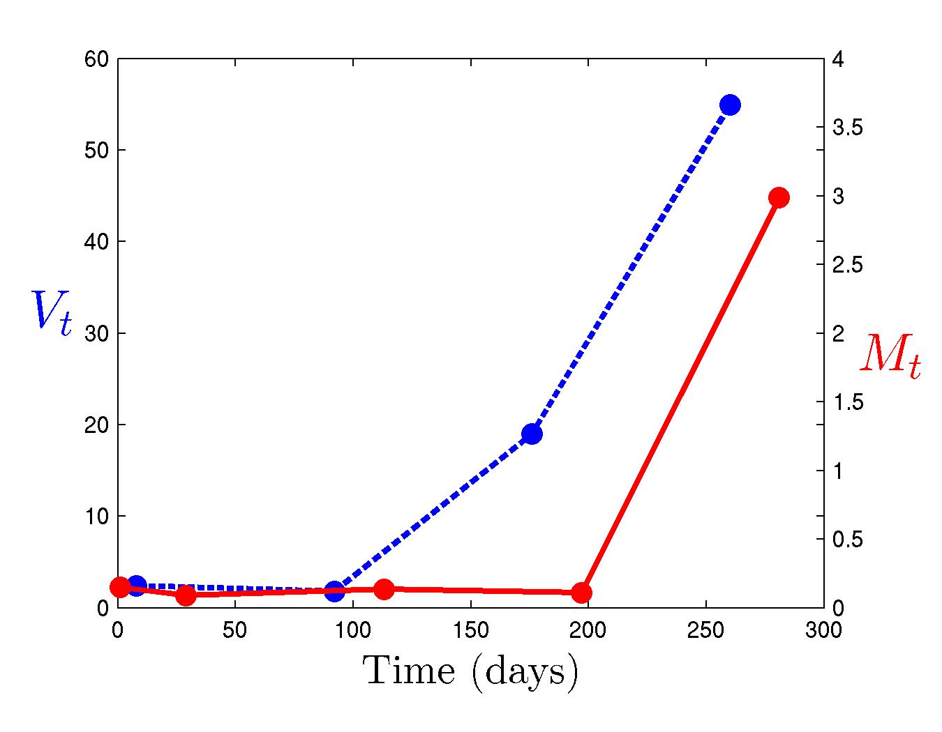
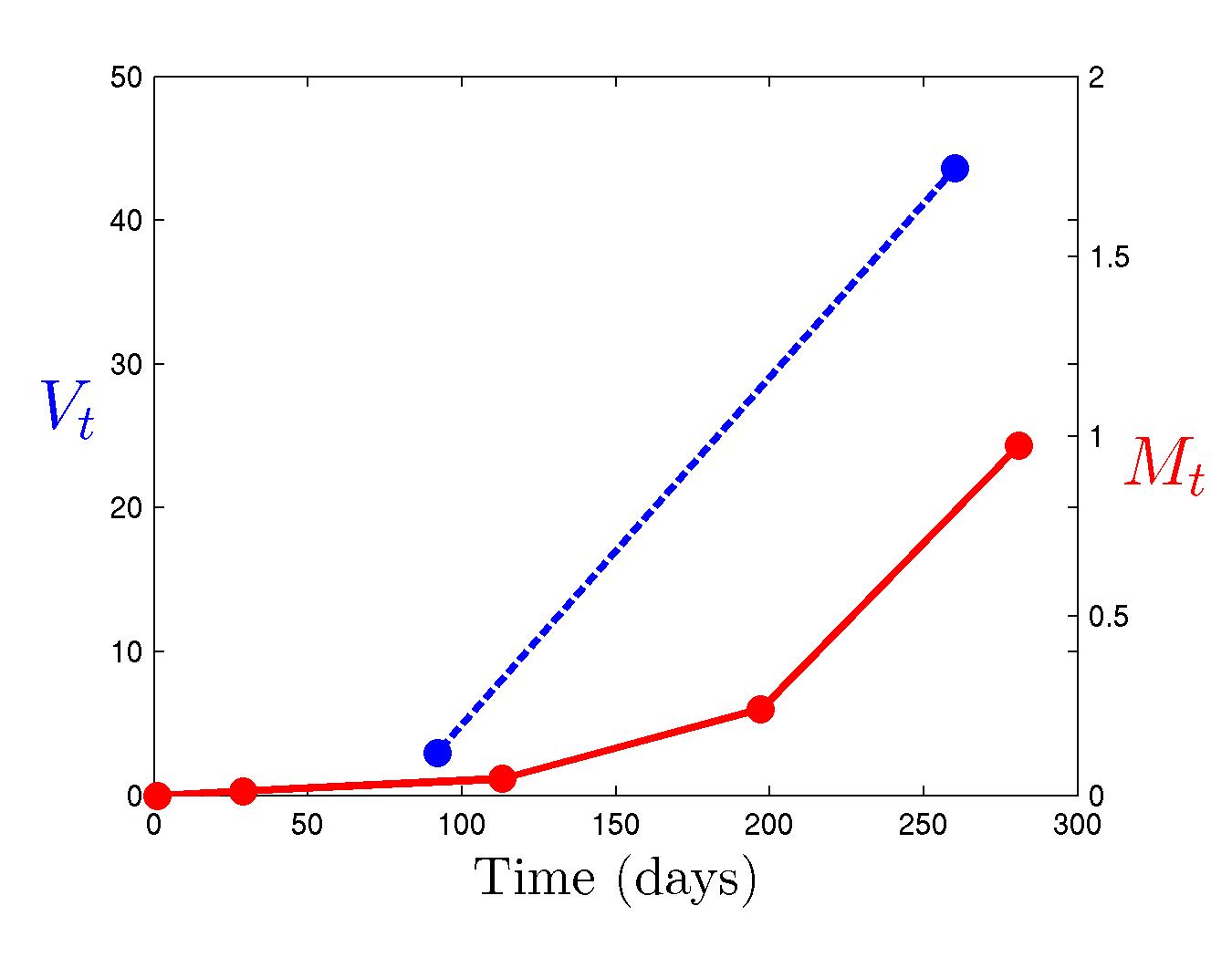
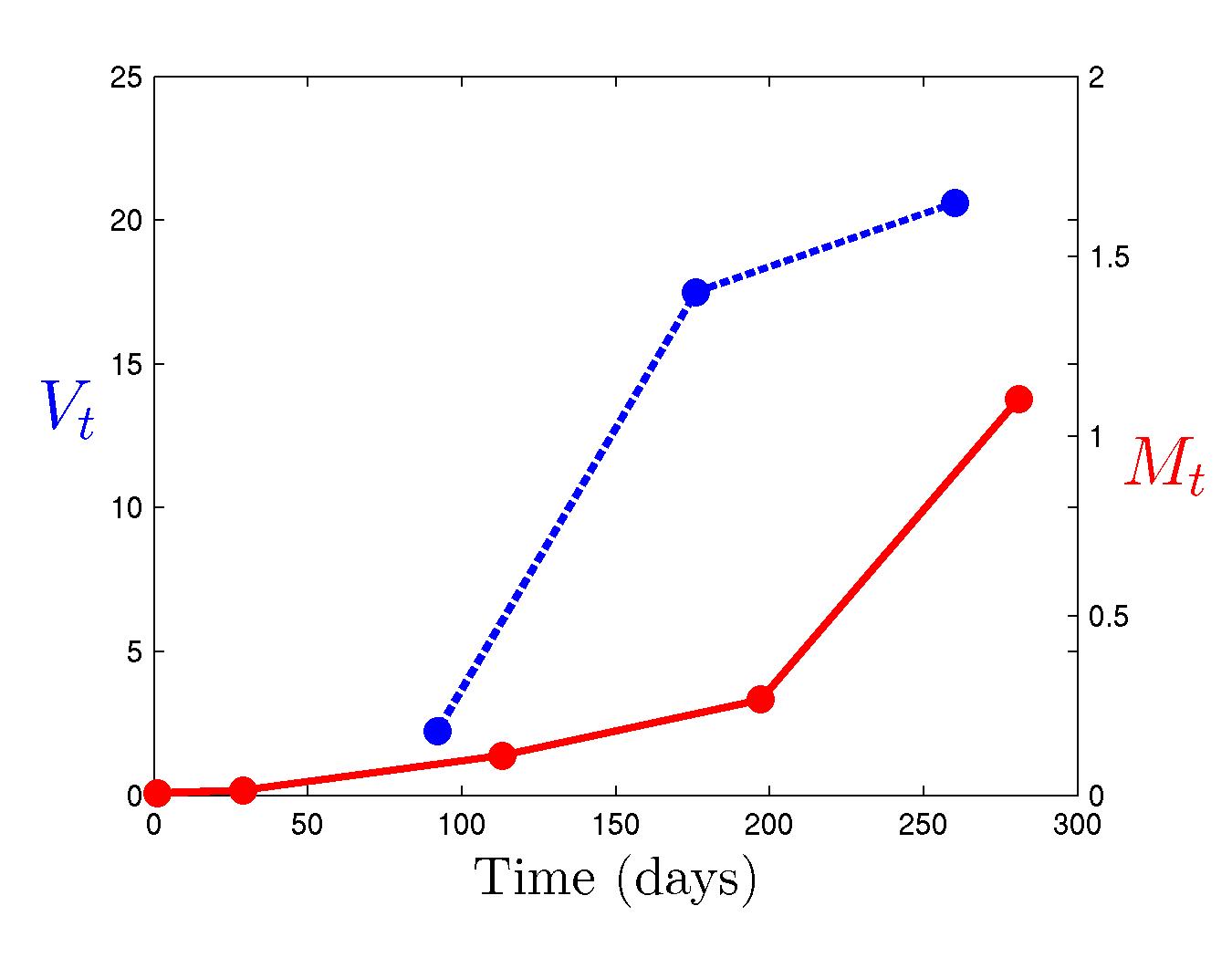
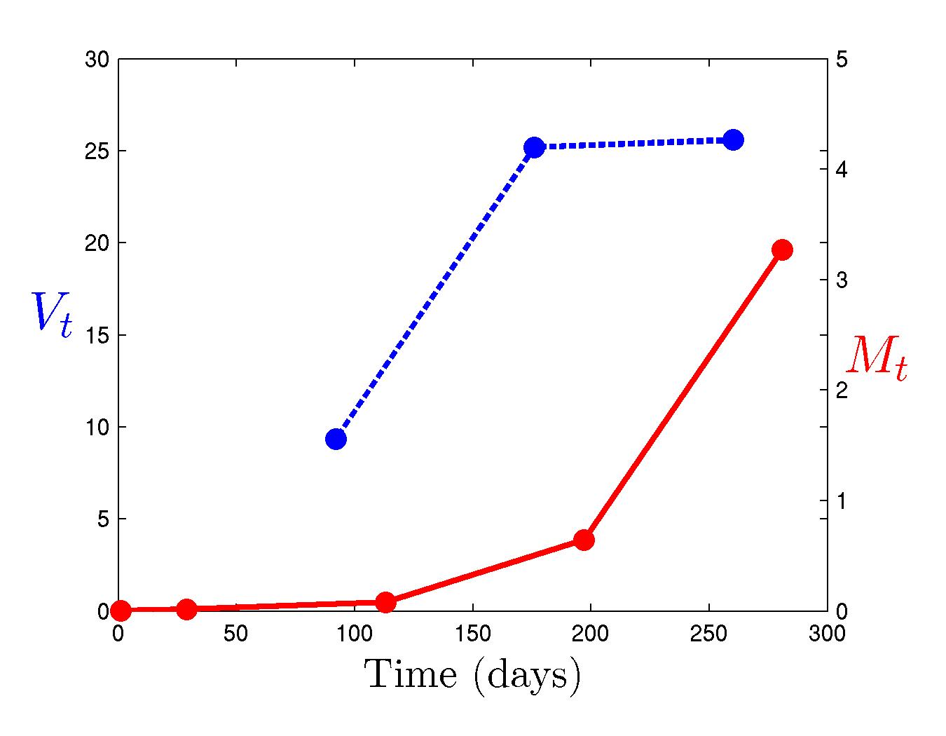
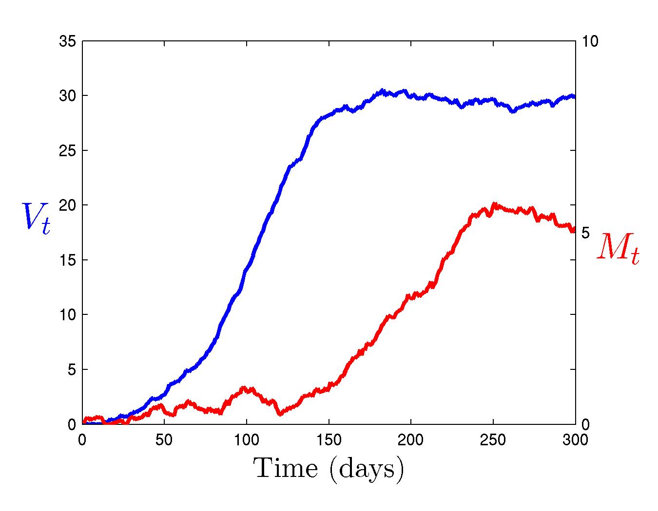
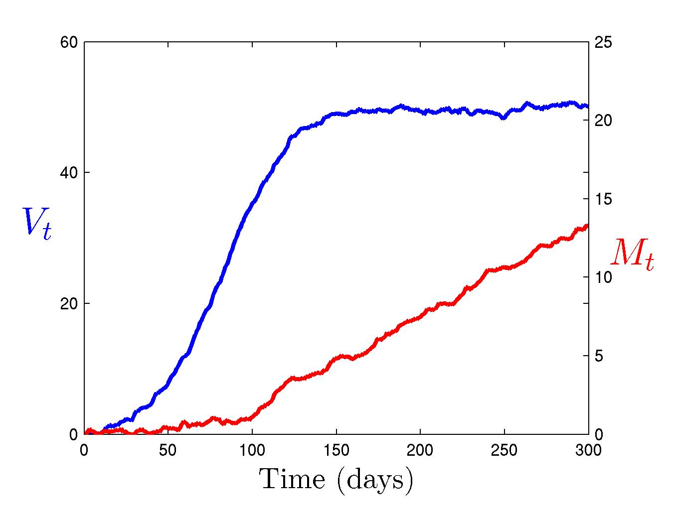
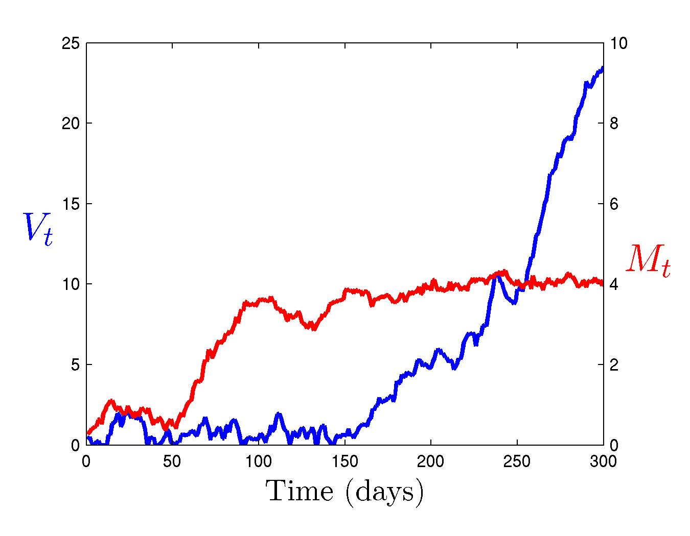
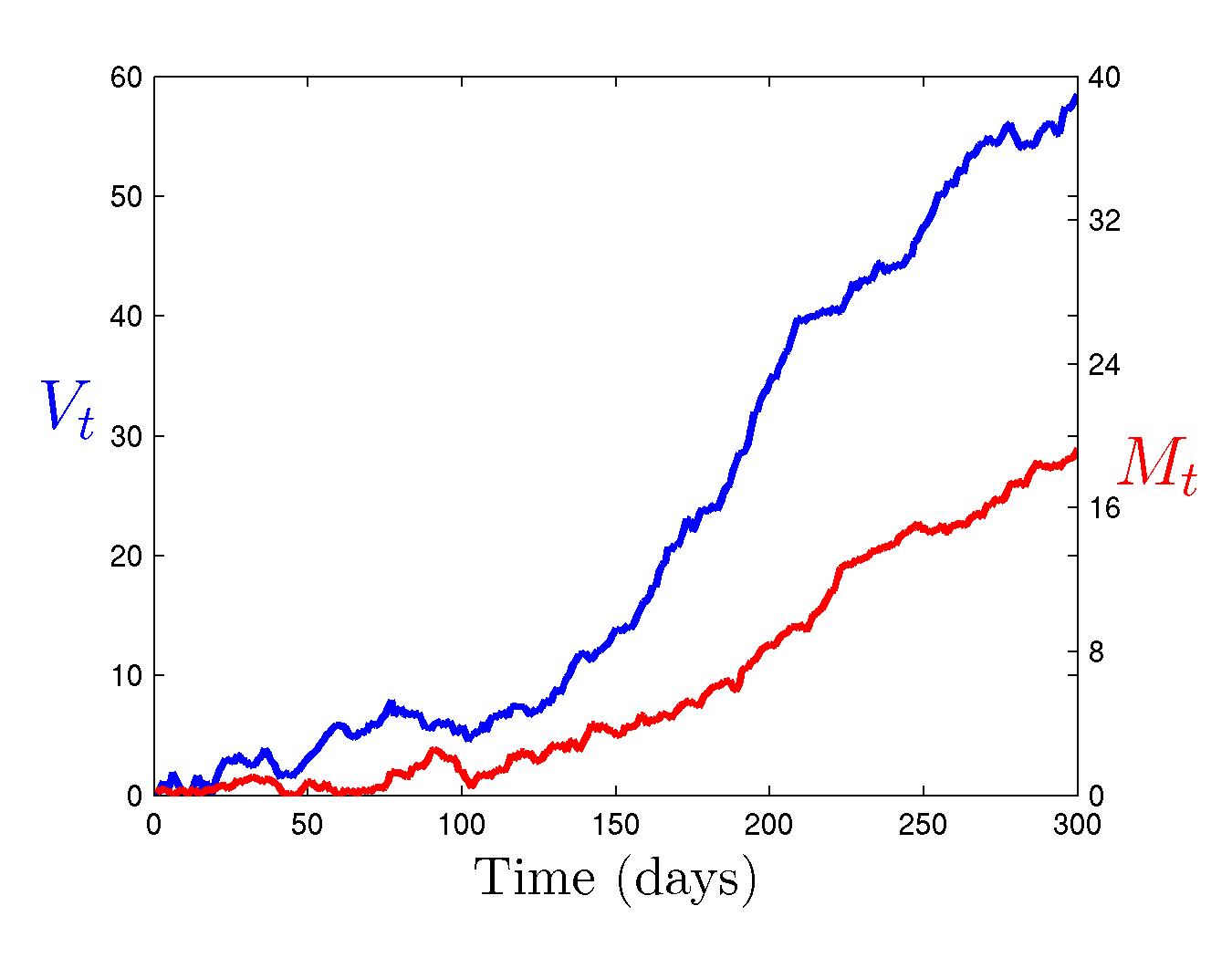
Figure 1: Observed data $V_{t}$ (blue) and $M_{t}$ (red) for 4 of the 8 macaques (subject IDs 400, 401, 404, 405, respectively).

Figure 2: Synthetic trajectories of $V_{t}$ (blue) and $M_{t}$ (red) from $(V_{0},M_{0})=(0.5,0.5)$, using model parameters chosen to be consistent with posteriors from the macaque study.

6 Analysis: HIV/SIV Study on Indian Rhesus Macaques

Data on 8 subject macaques was generated from flow cytometric analysis of GFP-labeled macrophages (i.e., Ad5 infected) from rectal mucosa sampled at weeks 1, 13, 25 and 37, together with the concentrations of gag-specific memory T-cells sampled at weeks 0, 4, 16, 28 and 40. Figure 2 shows the sparse time series of concentrations of viral population ($V_{t}$) and memory cells ($M_{t}$) on 4 macaques. The remaining 4 data sets are shown in the Supplementary Material. We perform separate analyses for each subject (macaque) and explore comparisons of inferences across subjects.

6.1 Model Predictions of Trajectories

To appreciate the relevance of the discrete-time, stochastic model with delay effects, we show representative trajectories in Figure 2. These are simply model simulations of $V_{t},M_{t}$ using plug-in parameter values that reflect the ranges we see in posteriors for some of the macaques, and is displayed here just to communicate that the model generates trajectories whose forms evidently match those of the data sets.

6.2 Priors

For the rate parameters $(\beta,\delta,\alpha,\rho,\gamma)$ we start with independent $U(0,1)$ priors, then impose constraints so that the carrying capacities $K_{v}=\beta/\delta$ and $K_{M}=\rho/\gamma$ are each less than 100%. Note that these are very diffuse priors. Priors for the variance parameters are independent, scaled inverse chi-squared on 5 degrees of freedom; their scale parameter are determined from analysis of data from other studies: $s_{\sigma^{2}_{V}}=0.4$, $s_{\sigma^{2}_{M}}=0.08$, $s_{\kappa^{2}_{V}}=0.05$, $s_{\kappa^{2}_{M}}=0.01$. For the time discretization, we take $h=1$day and the priors for time delays $\tau_{V},\tau_{M}$ are independent discrete uniforms on $\{1,\ldots,50\}$. The initial viral level $V_{0}$ has a $U(0,0.5)$ prior, and $M_{0}$ is fixed at a value based on initial measurements for each macaque.

6.3 Bayesian Computations

The two stage analysis ran MCMC chains 10,000 iterations with a burn-in of 3,000. The weighted ABC analysis generated 10,000 accepted particles. Following standard practice [e.g., 19, 1, 2], the threshold level $\epsilon$ was set based on the discrepancy value that separated the closest 5% of synthetic data sets to $\mathbf{Y}_{o},$ using $d(\mathbf{Y},\mathbf{Y}_{o})=\sum_{t\in O_{V}}(y_{Vt}-y_{oVt})^{2}/s_{V}^{2}+\sum_{t\in O_{M}}(y_{Mt}-y_{oMt})^{2}/s_{M}^{2}$, where $s_{V}$ and $s_{M}$ are the standard deviations of the observed values $y_{oV},y_{oM}$, respectively.

6.4 Some Posterior Summaries for Parameters

Figure 3 summarizes marginal posteriors from analysis of data on one macaque; these are typical of all 8 analyses. Evidently, some concentrated heavily in small regions relative to the diffuse initial $U(0,1)$ priors; e.g., see rate parameters $\beta,\alpha,\rho,\delta$ and $\gamma$. Margins for the carrying capacity parameters, $K_{V}$ and $K_{M}$ are also quite informative, while those for $V_{0}$ and the delays $\tau_{V},\tau_{M}$ are more diffuse while still contrasting somewhat with their uniform priors. Figure 4 shows summaries for selected bivariate margins, evidencing some posterior dependencies between rate parameters in the posterior distribution.

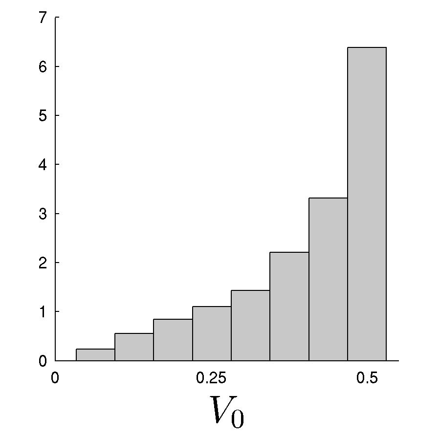
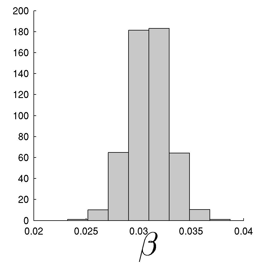
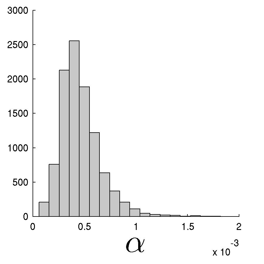
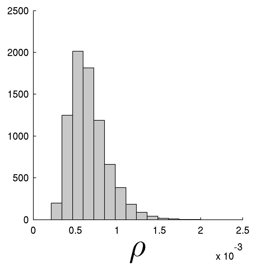
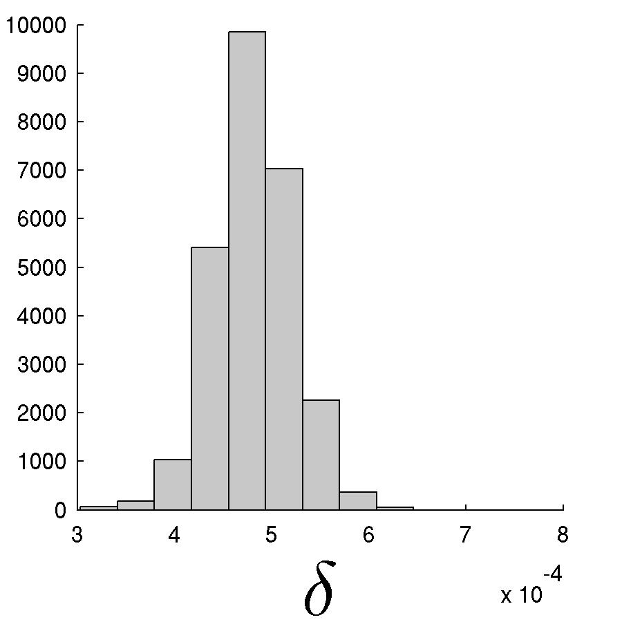
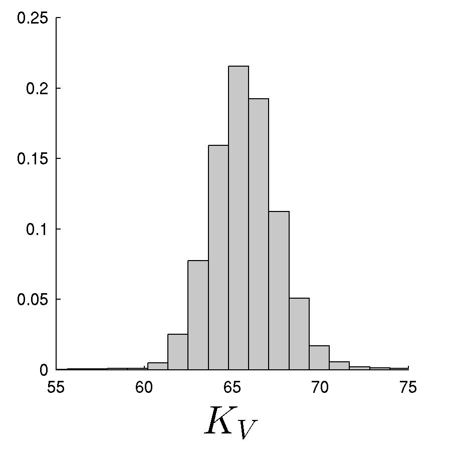
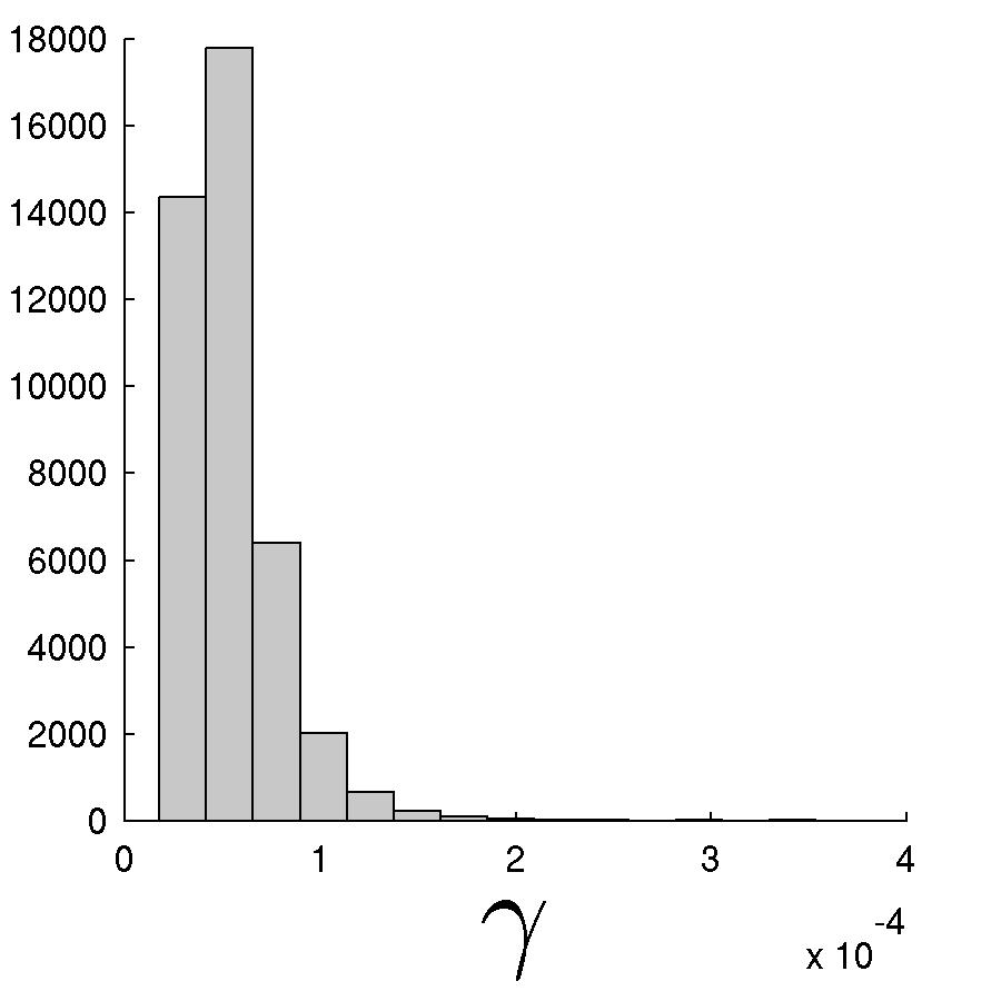
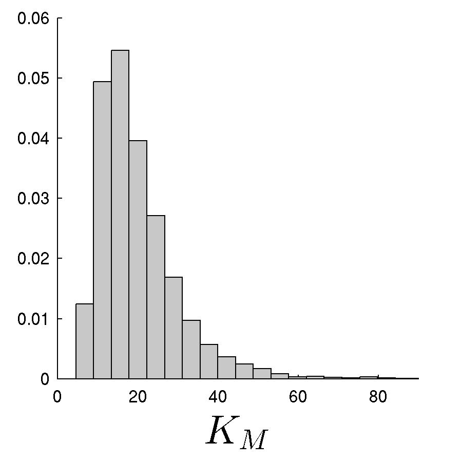
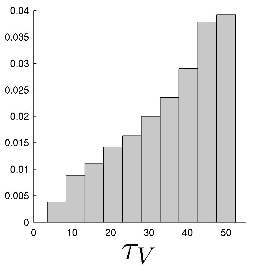
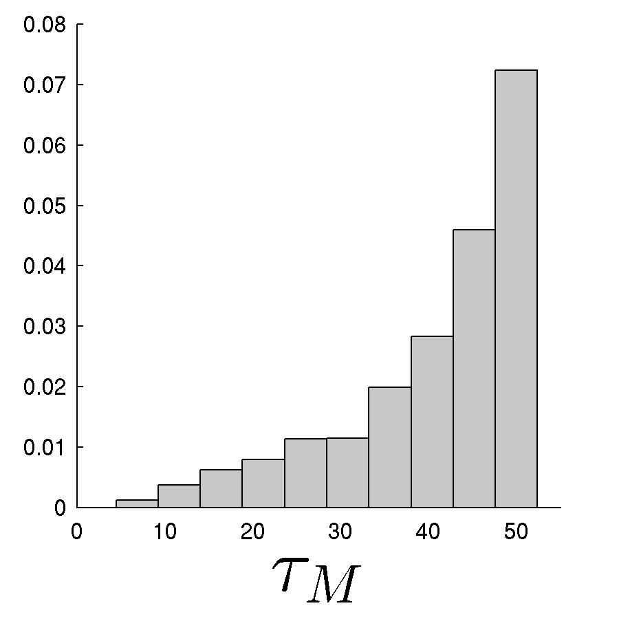
Figure 3: Macaque 400: posterior margins for the 10 parameters as annotated.

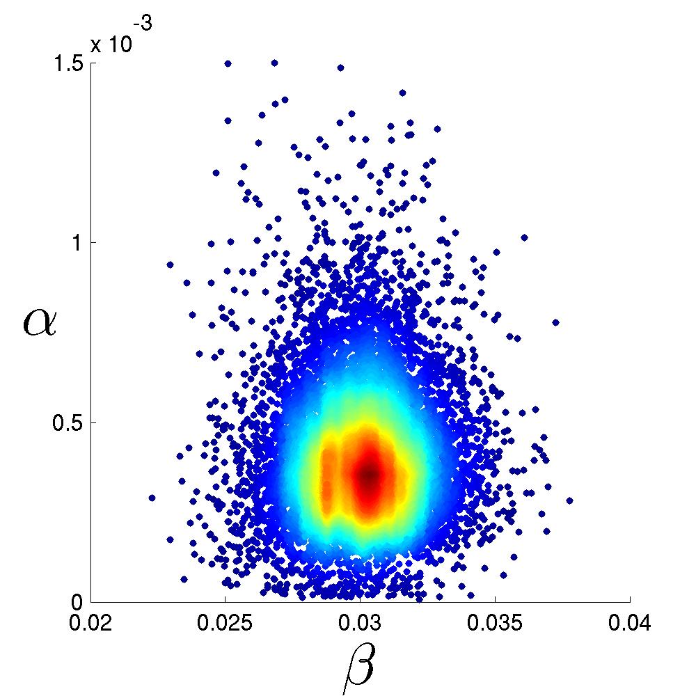
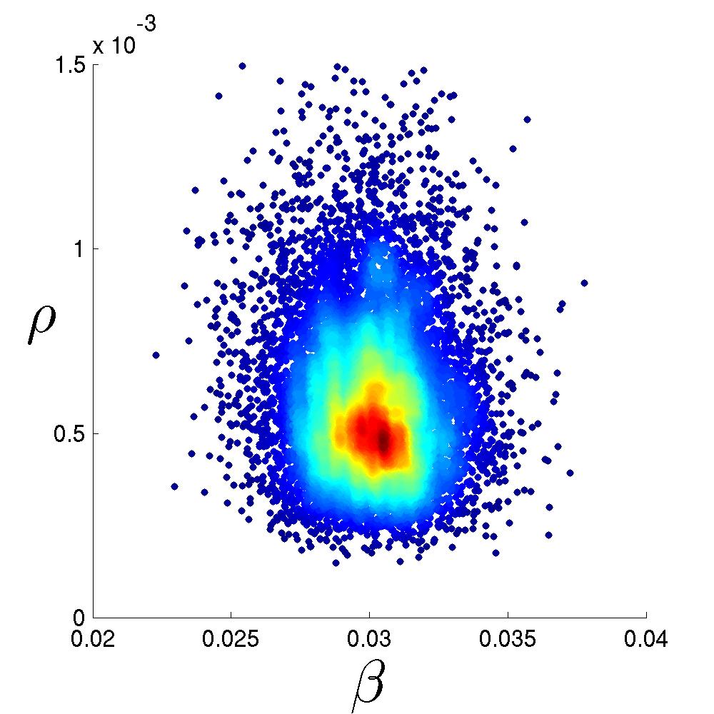
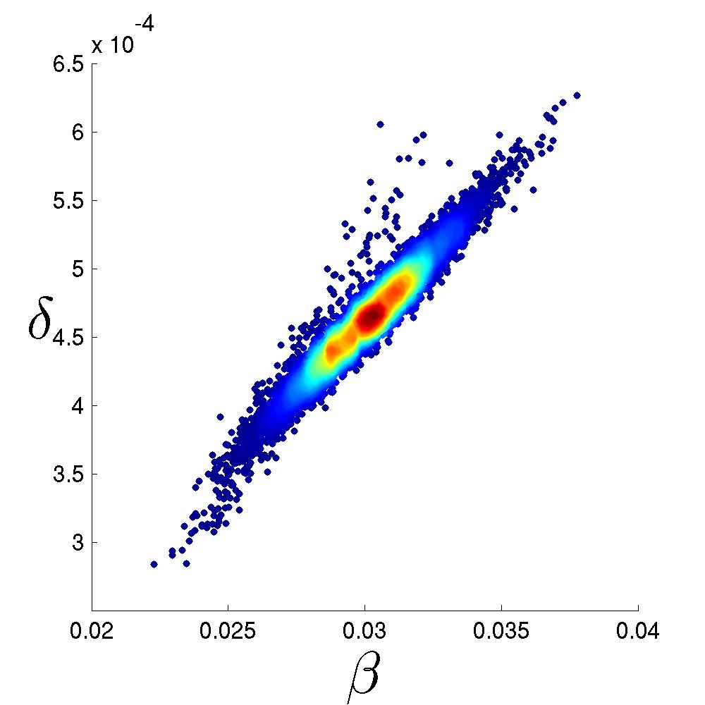
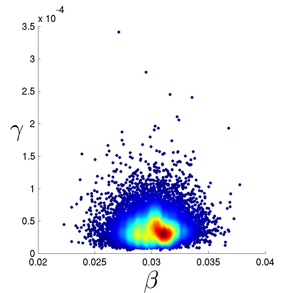
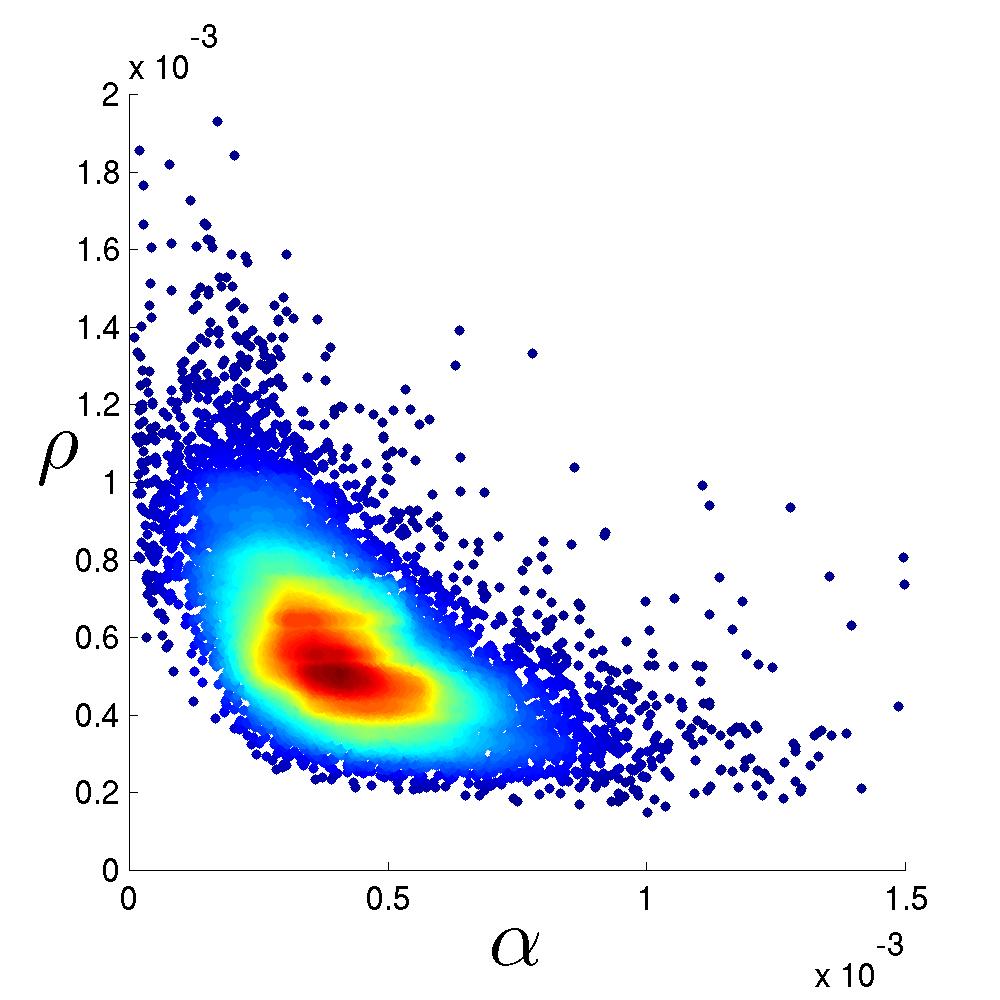
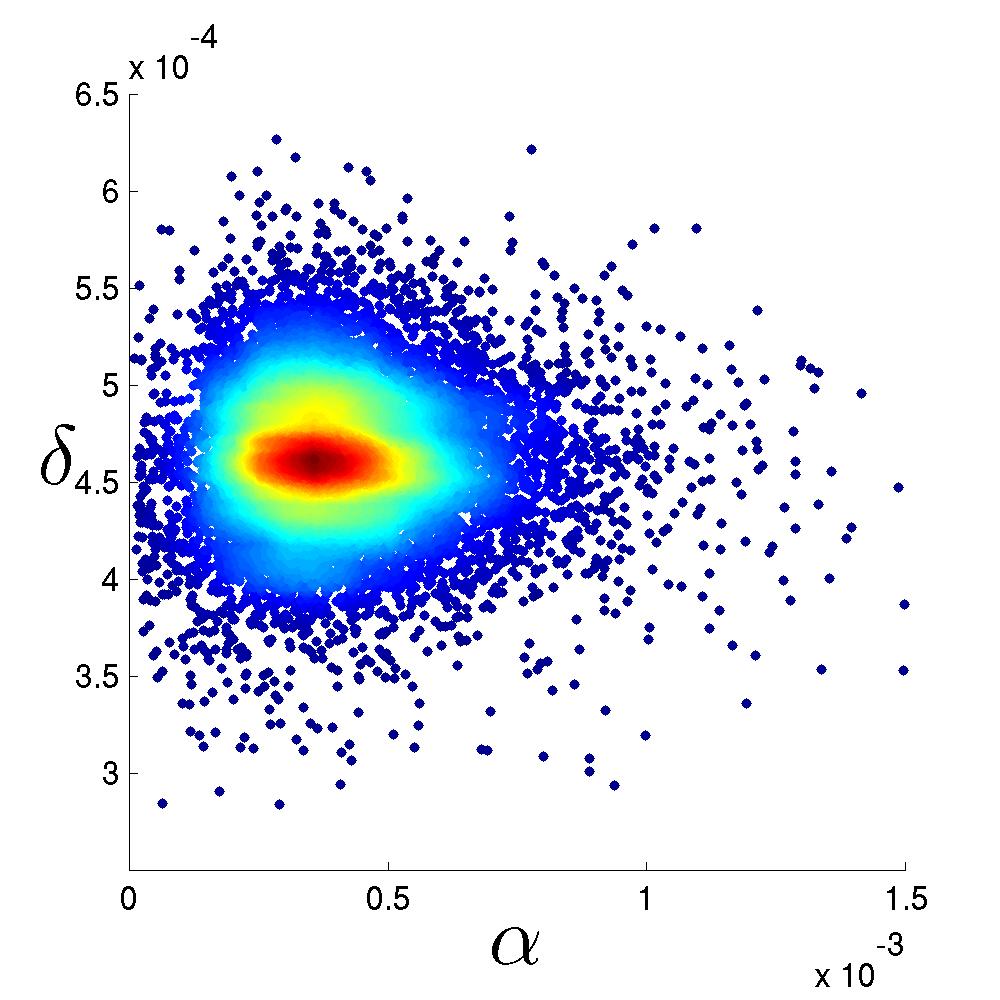
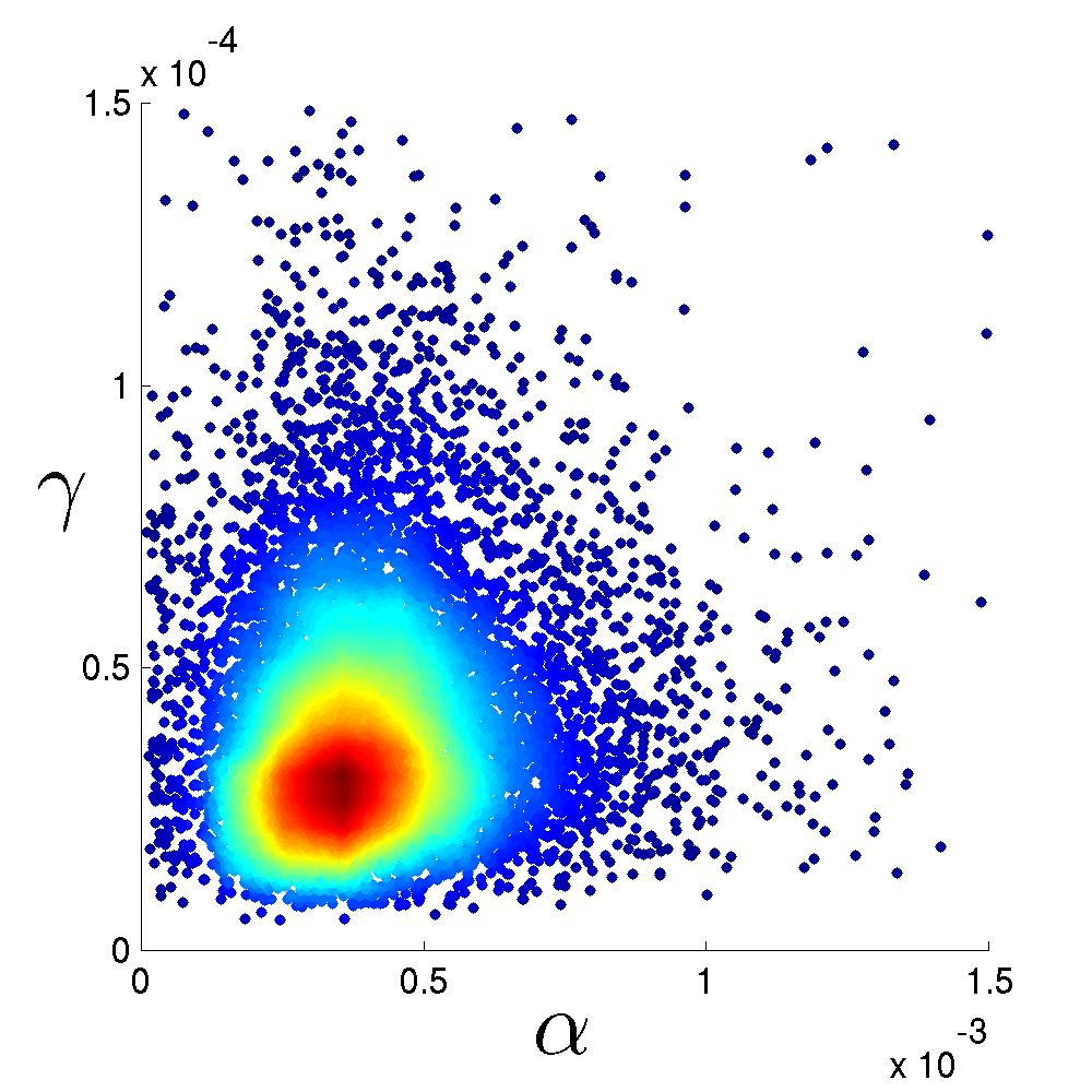
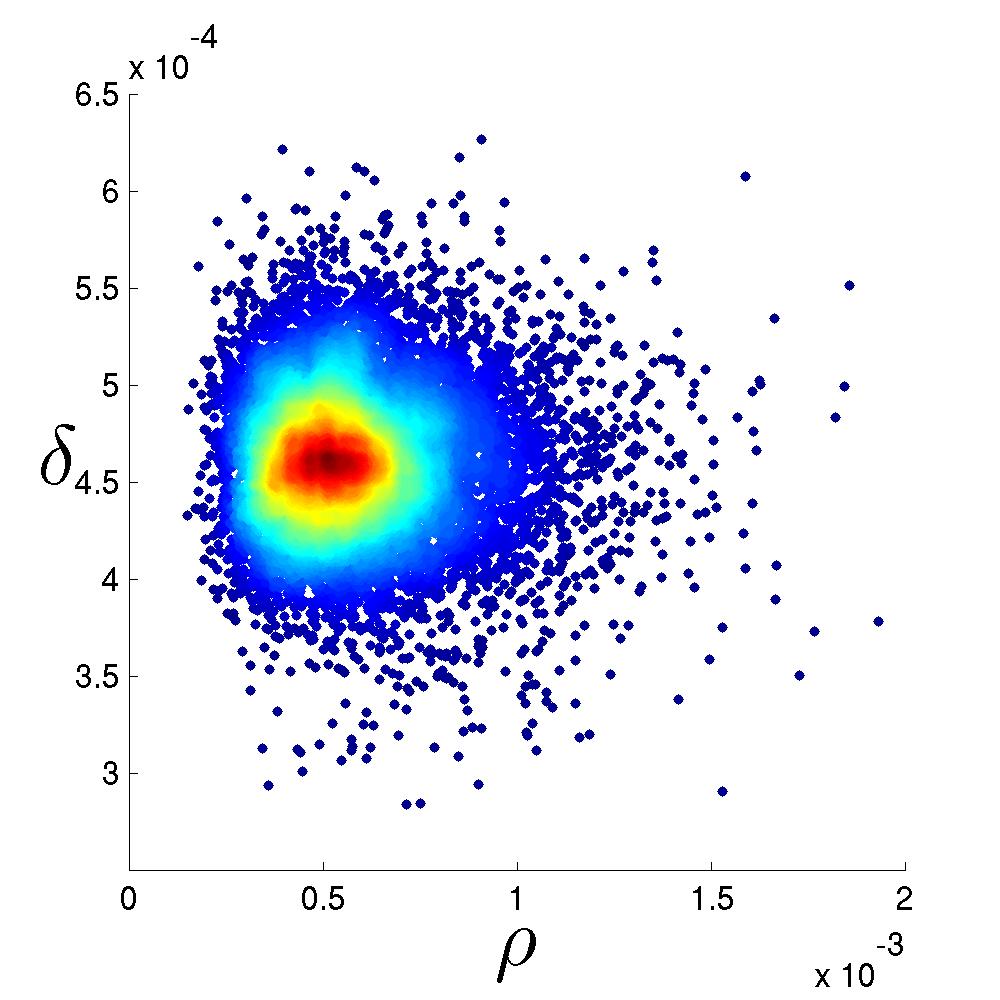
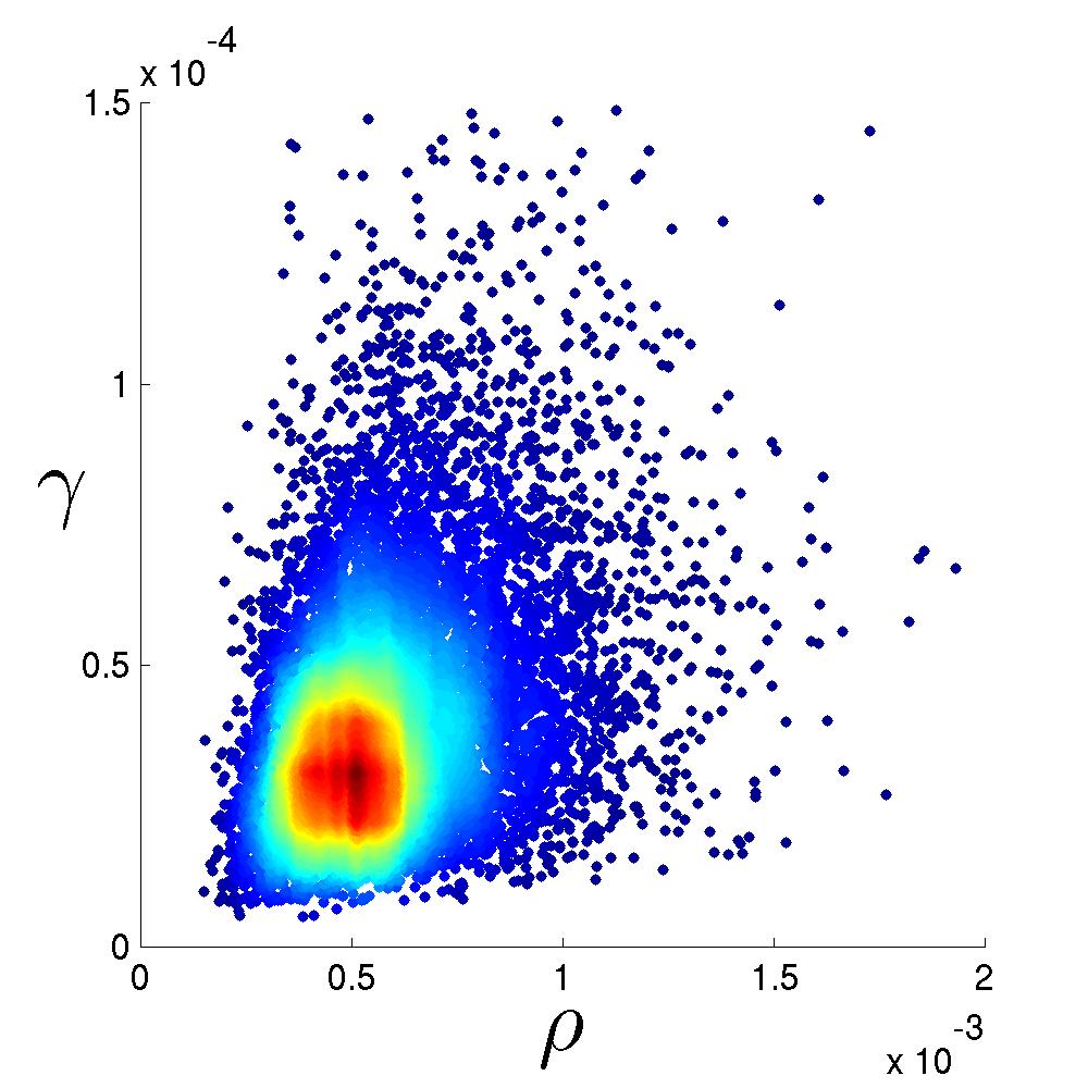
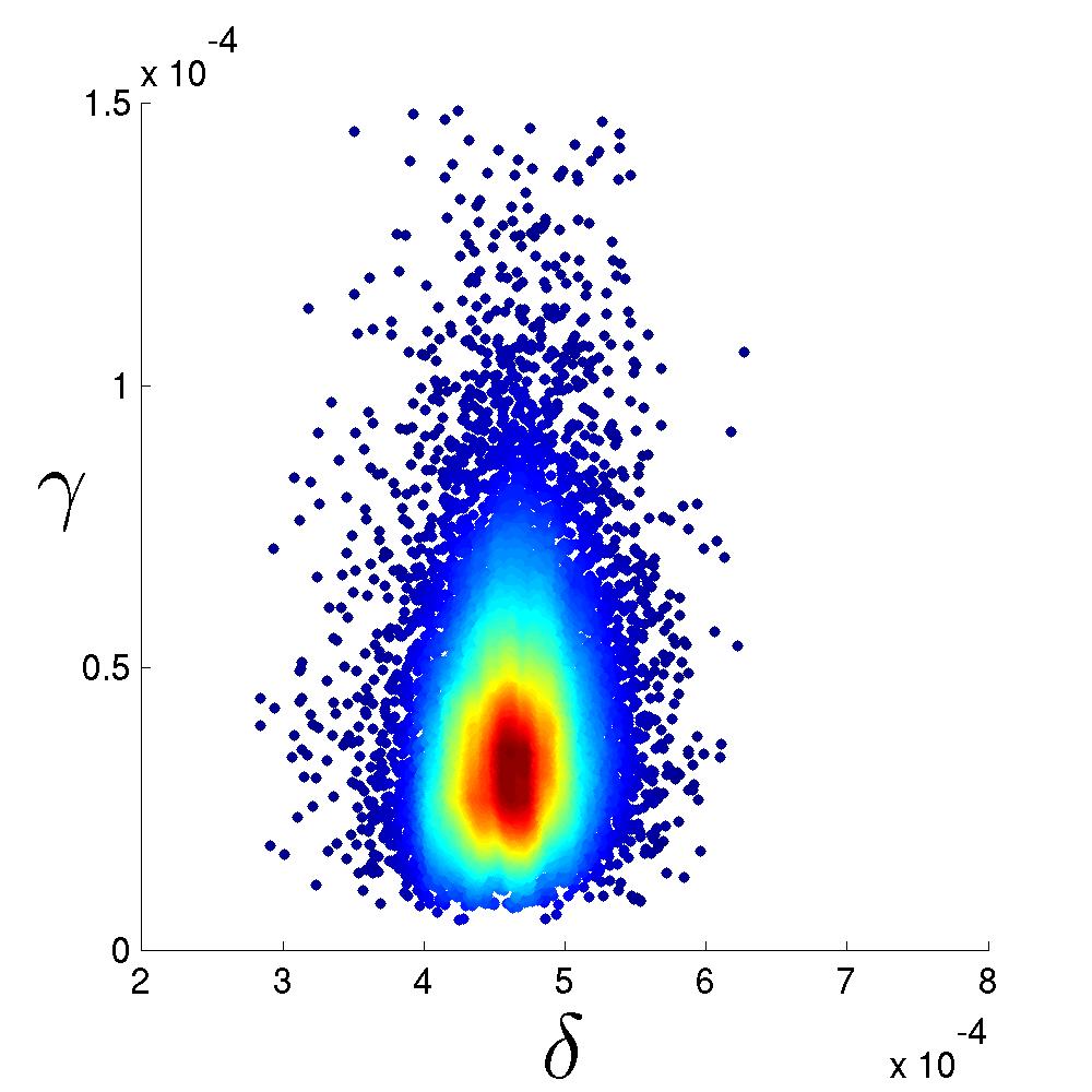
Figure 4: Macaque 400: bivariate posterior margins for the 10 parameters as annotated.

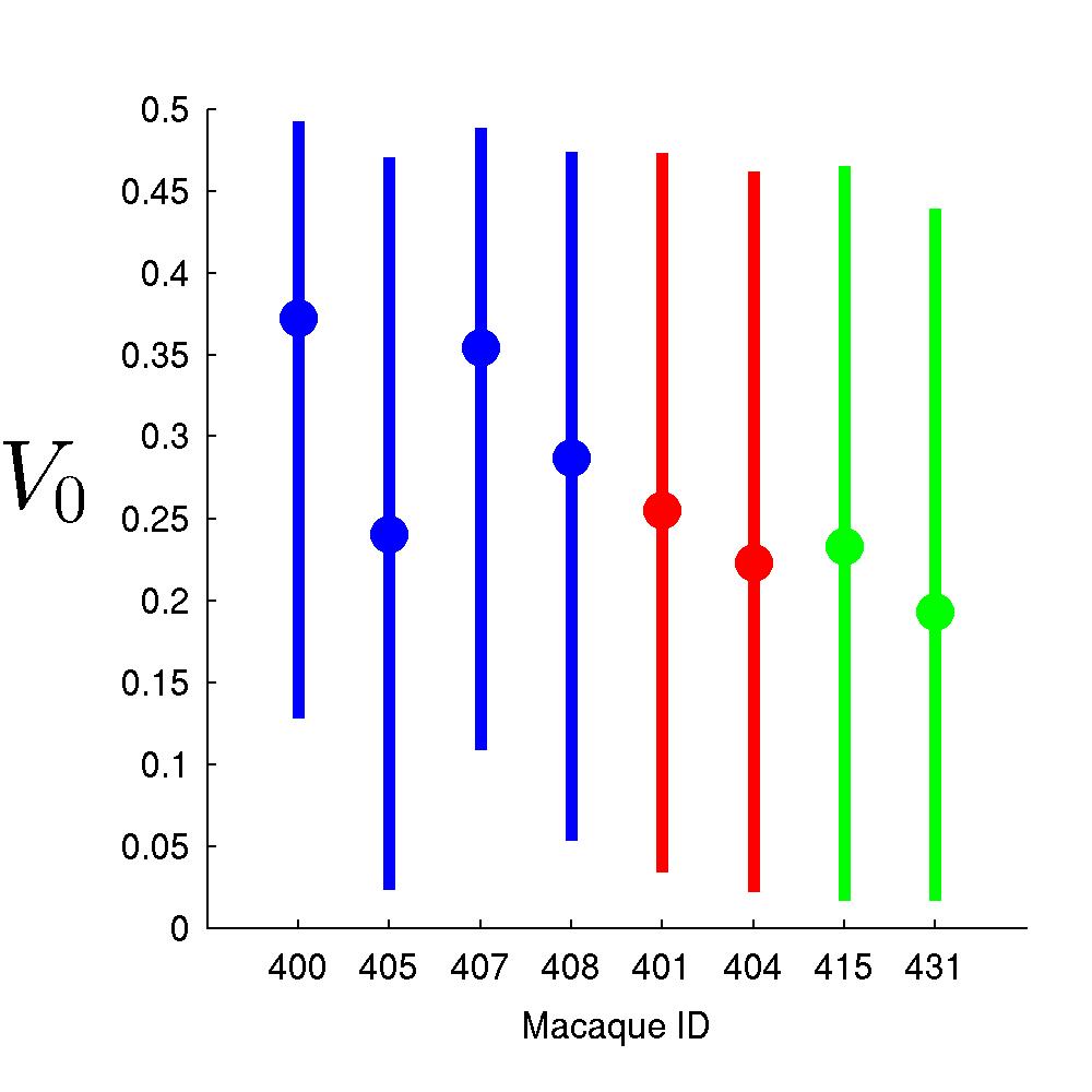
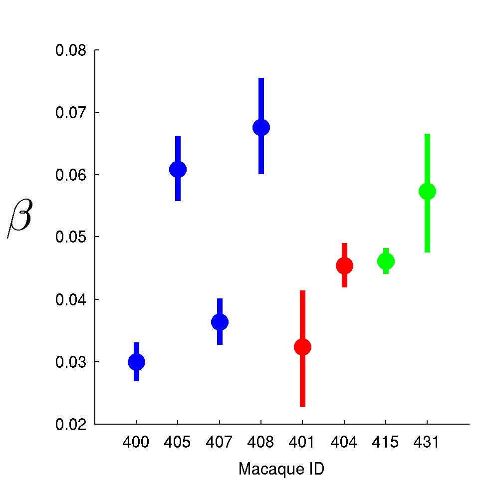
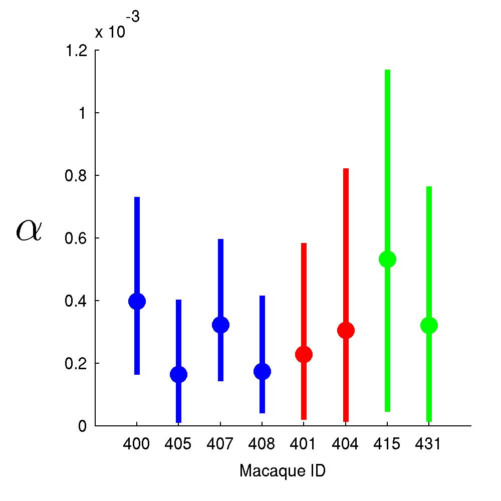
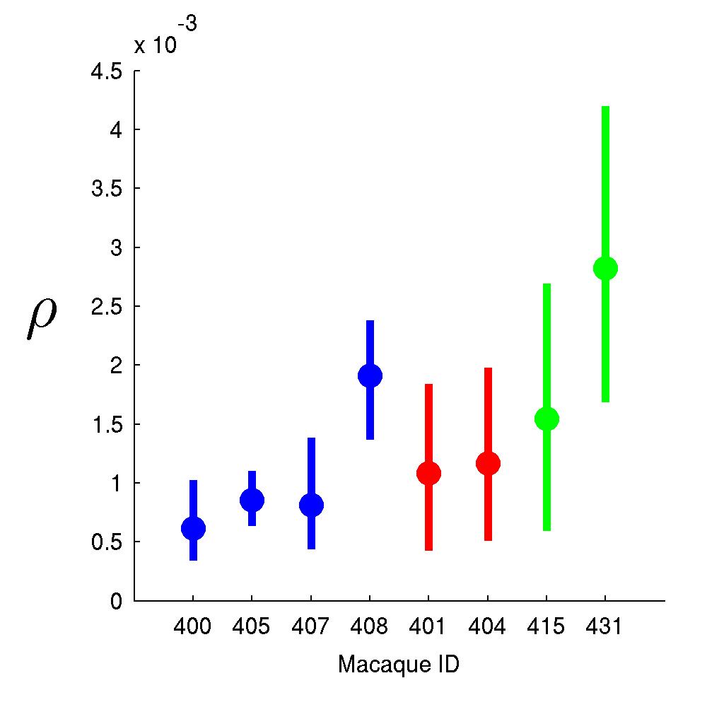
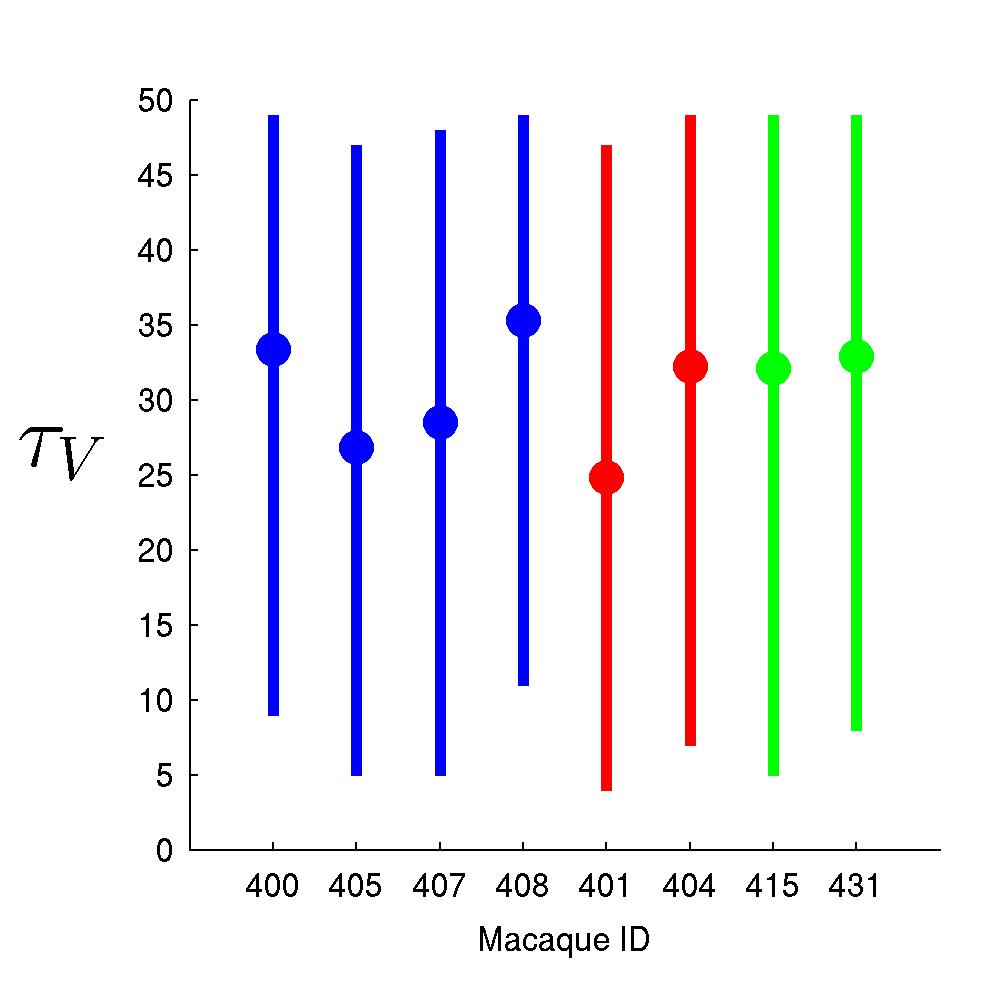
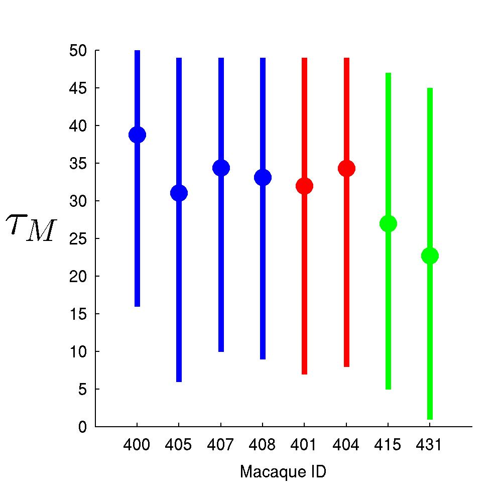
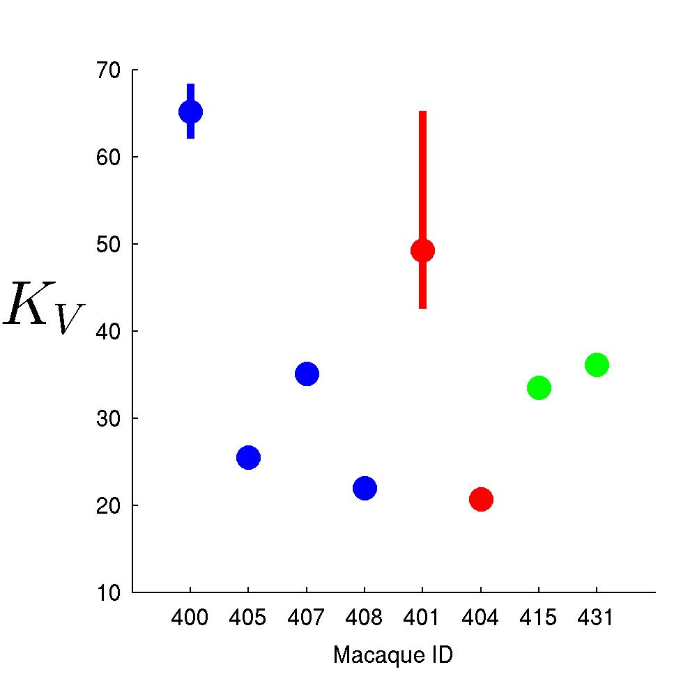
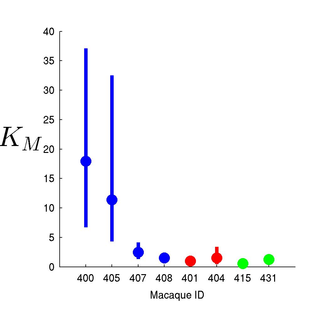
Figure 5: Marginal posterior means and 90% credible intervals for key parameters on all 8 macaques. Color reflects vaccine immunization route: intra-nasal/intra-tracheal (blue), intra-rectal (red), intra-vagina (green).

6.5 Comparisons of Subjects and Vaccination Routes

Figure 5 provides marginal posterior summaries to compare across the 8 macaques. In general, there is substantial learning for the rate parameters $\beta,\alpha$, and $\rho$, and for the carrying capacity parameters, $K_{V}$ and $K_{M}$. The extent of learning is dependent on the conditions of the experiment, evidenced by the varying widths of credible intervals. For three parameter – the initial viral level $V_{0}$ and delays $\tau_{V},\tau_{M}$– such sparse time series data is generally relatively uninformative: posteriors resemble priors on these quantities.

Color coding relates to immunization route of the vaccine administered– intra-nasal/intra-tracheal, intra-rectal, or intra-vaginal. For $\rho,K_{M},$ there is some indication of differences by immunization route, which was unanticipated. Additional experiments directed towards comparing finer-scale immune responses across immunization route are suggested as a result.

6.6 MCMC+ABC Improves Predictive Model Fit

Posterior predictions assess and compare model fits; these demonstrate the positive benefit of the ABC procedure in refining the first stage MCMC analysis. For each data set, final posterior parameter samples were used to generate synthetic latent state trajectories. Figures 6 shows aspects of these predictions for macaque #400. These posterior predictive trajectories were simulated (i) based on the first stage MCMC alone, and (ii) from the full MCMC+ABC analysis. This shows that the MCMC analysis results in a relatively good concordance with the data; however, systematic bias in overestimating the latent states is clear– likely a result of linearization and lack of truncation in the MCMC analysis. The figure shows how the ABC step is able to “correct” this, resulting in clear improvements in predictive fit.

Repeating this comparative analysis for the other 6 data sets leads to similar conclusions; see graphs in the Supplementary Material. For some cases, very clear improvements are evident. For a few, such as macaque #401, there is less evidence of systematic bias in the MCMC analysis, and then the ABC step results in minimal adjustment.

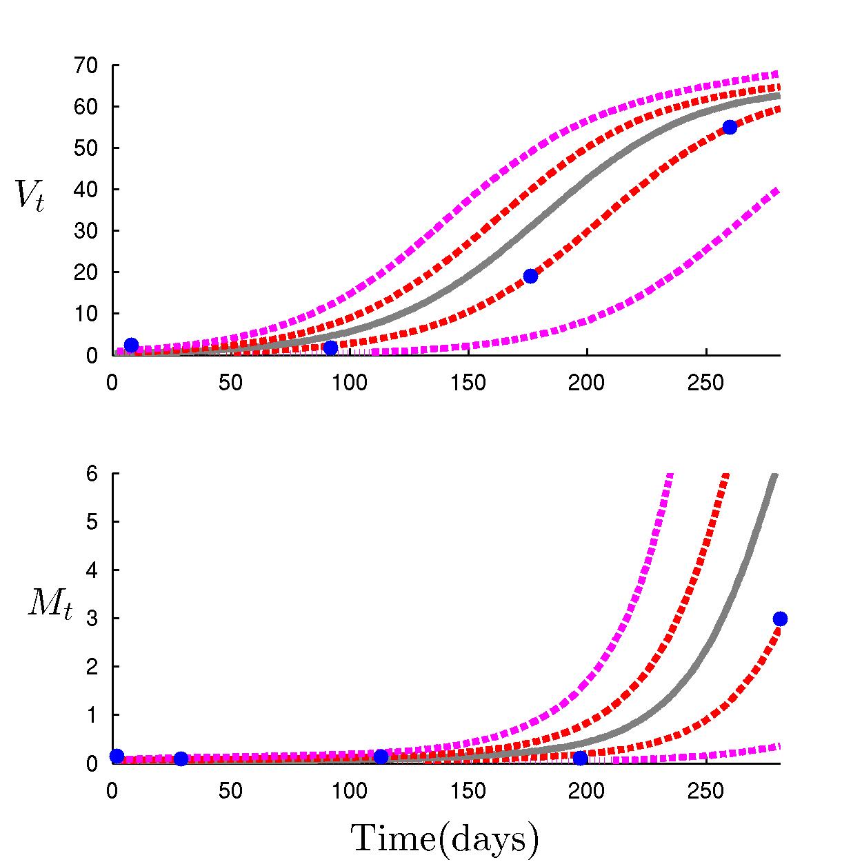
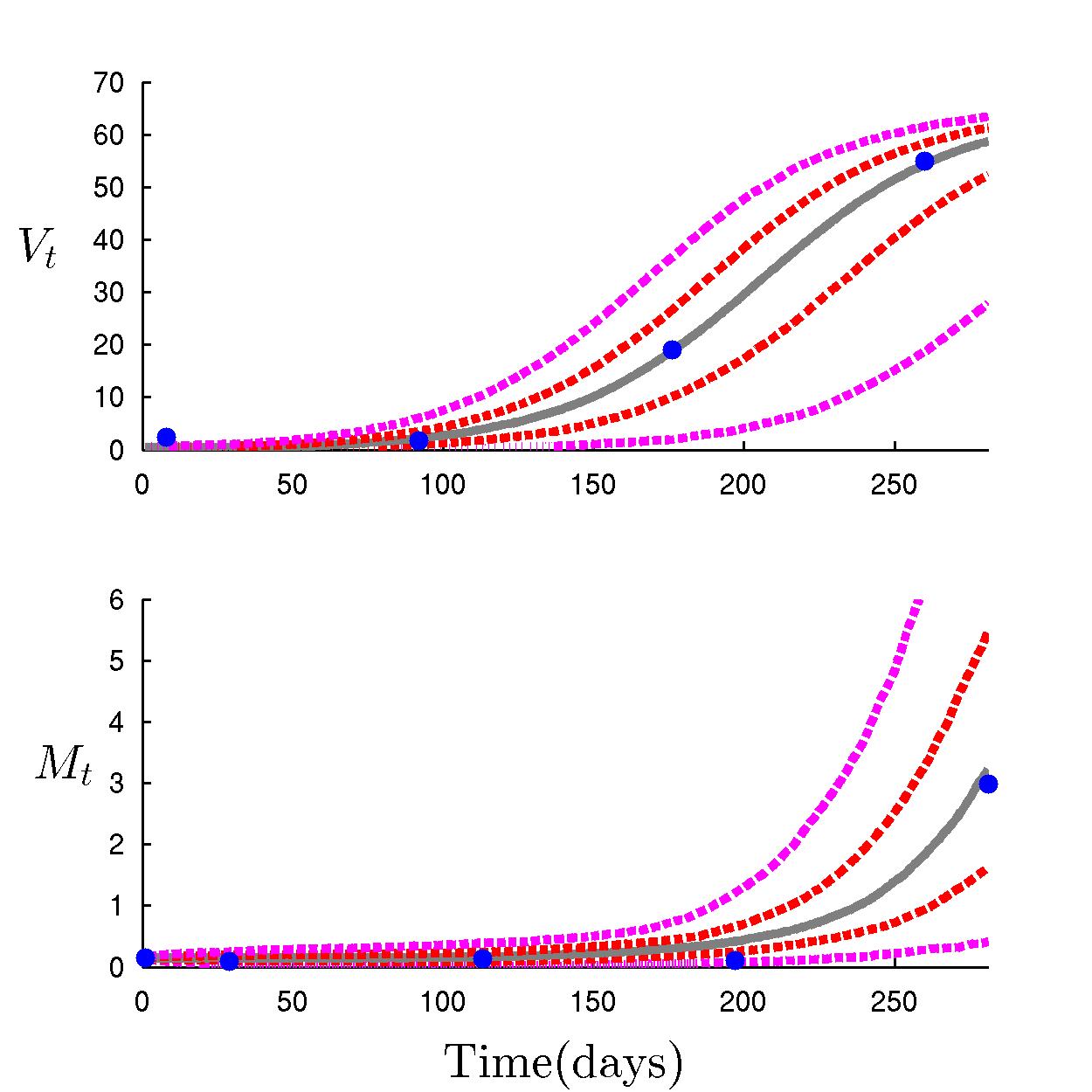
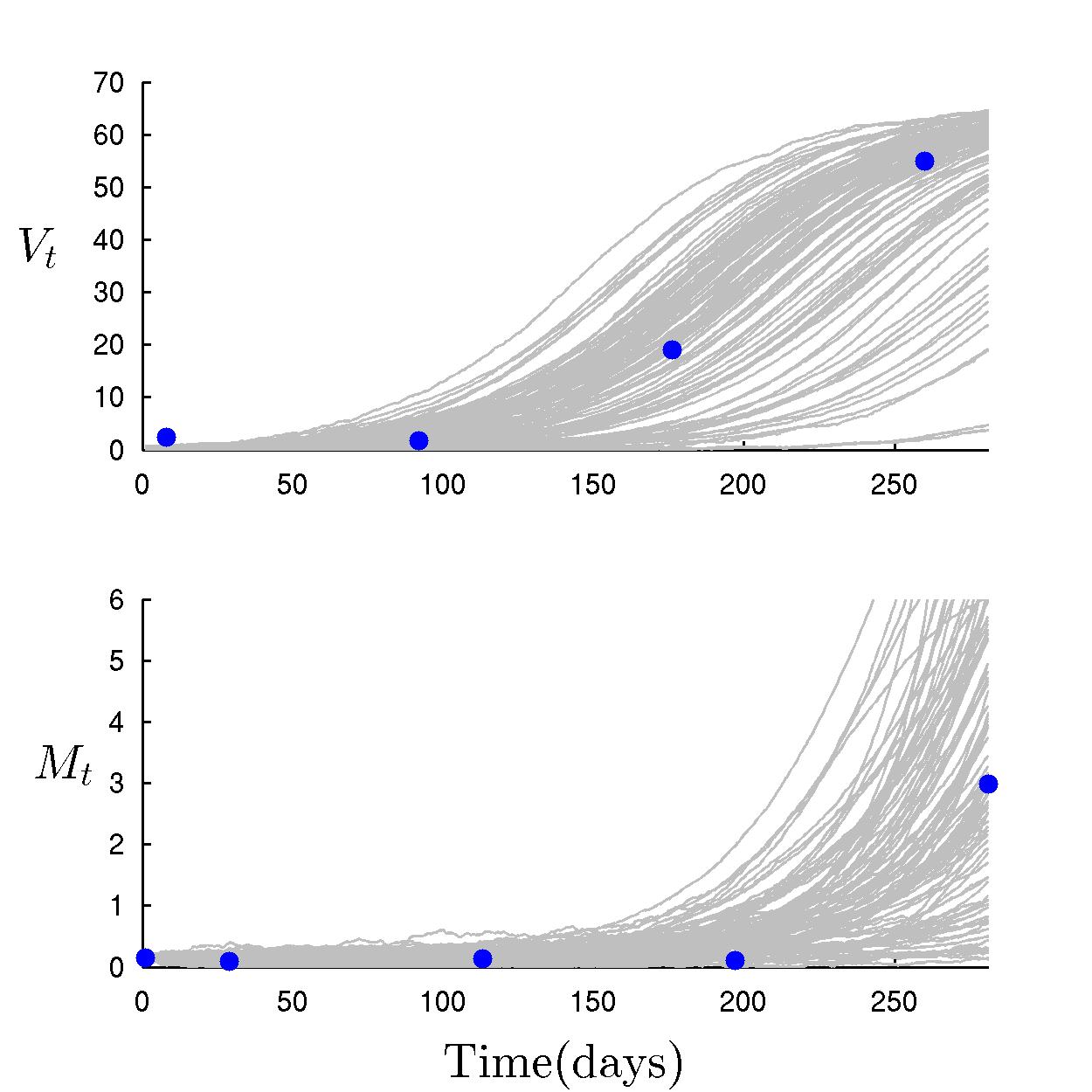
Figure 6: Posterior predictions for macaque #400: Top left: Observed data (blue); 50% (red), 95% (magenta) credible bands and median (gray) of posterior predictions for the latent states using only MCMC analysis. Top right: Same format, but based on MCMC+ABC analysis. Lower center: 100 sample trajectories from the posterior predictive distribution of the latent states from MCMC+ABC analysis.

6.7 Comparisons via Dimensionless Model Parameters

The dimensionless form of equation (2) is a “canonical skeleton” of the non-linear model. We can compare across experiments in terms of (i) the dimensionless parameters $\eta=\alpha\beta/(K_{V}K_{M})$ and $\psi=\rho K_{V}/\beta$, and (ii) the transformed time scale $s=\beta t.$ Also, from Section 4.1, the implied transformed time delays are $\lambda_{V}=\beta\tau_{V}$ and $\lambda_{M}=\beta\tau_{M}.$ Figure 5 already shows major differences across macaques in the posteriors for $\beta$, indicating substantial differences in effective time scales of immune responses across subjects. For the other dimensionless parameters, we simply transform the MCMC+ABC posterior samples to approximate posteriors for $(\eta,\psi,\lambda_{V},\lambda_{M})$ to study what has been learned about these “canonical” parameters and how they compare across subjects. Figures 7,8,9 show marginal and bivariate posteriors for macaque #400, and credible interval summaries for these 4 quantities on all 8 macaques; the latter shows up evident differences across macaques, especially for $\eta,\psi.$

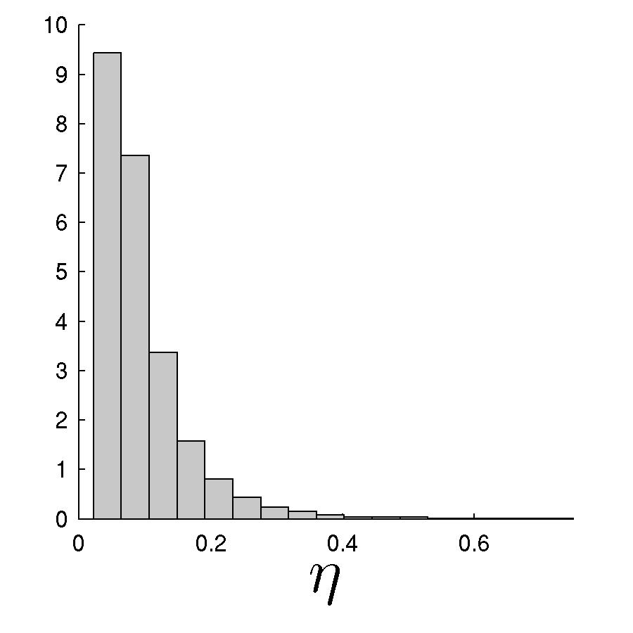
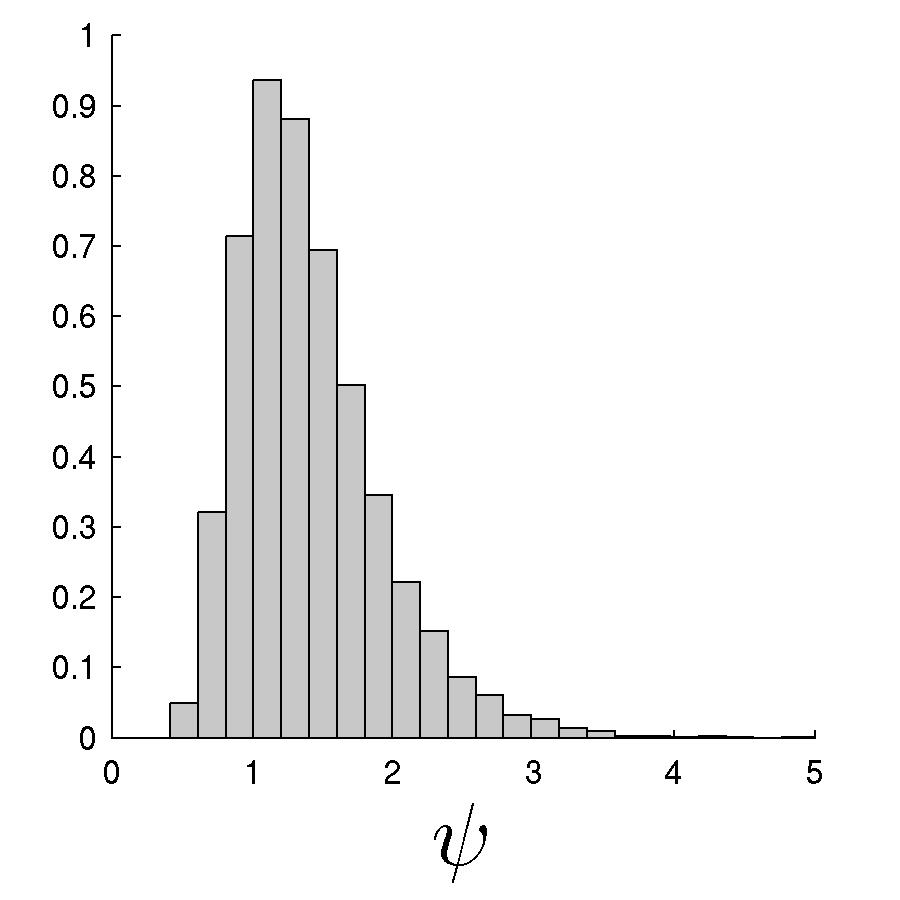
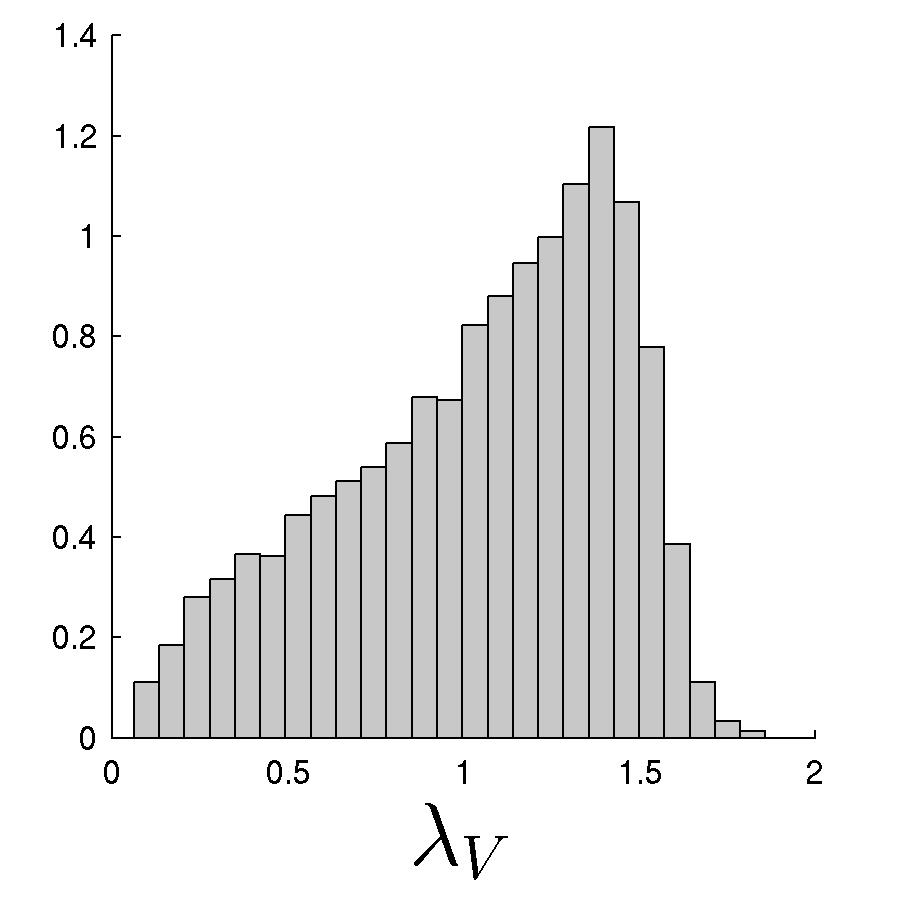
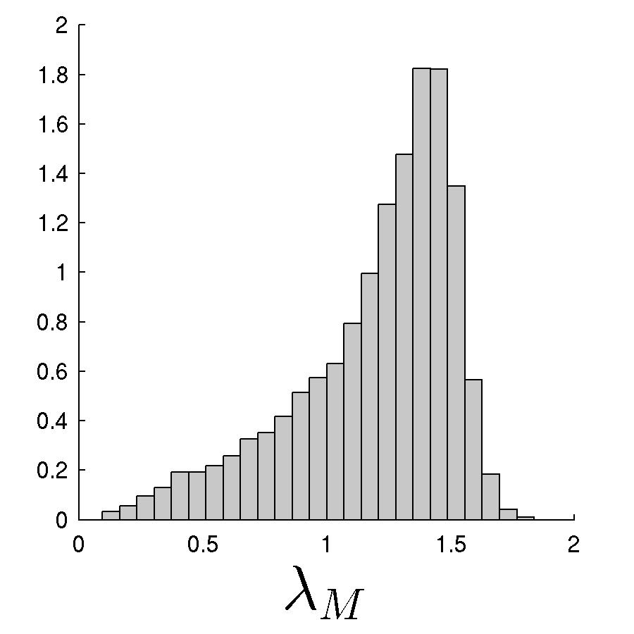
Figure 7: Macaque 400: posterior margins for the for the dimensionless model parameters as annotated.

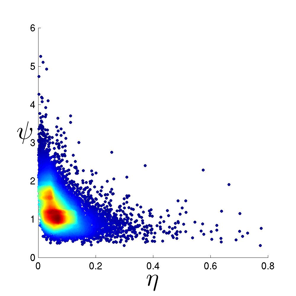
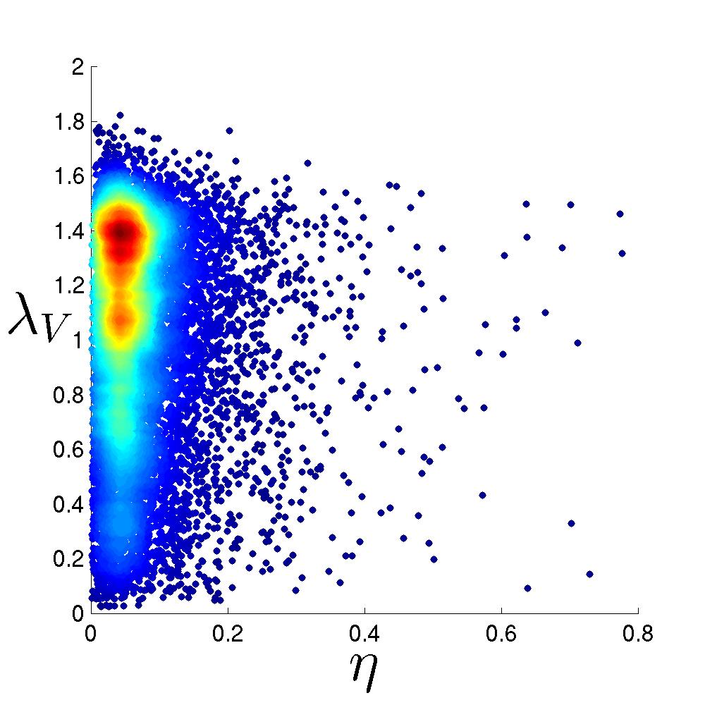
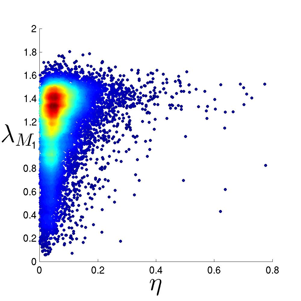
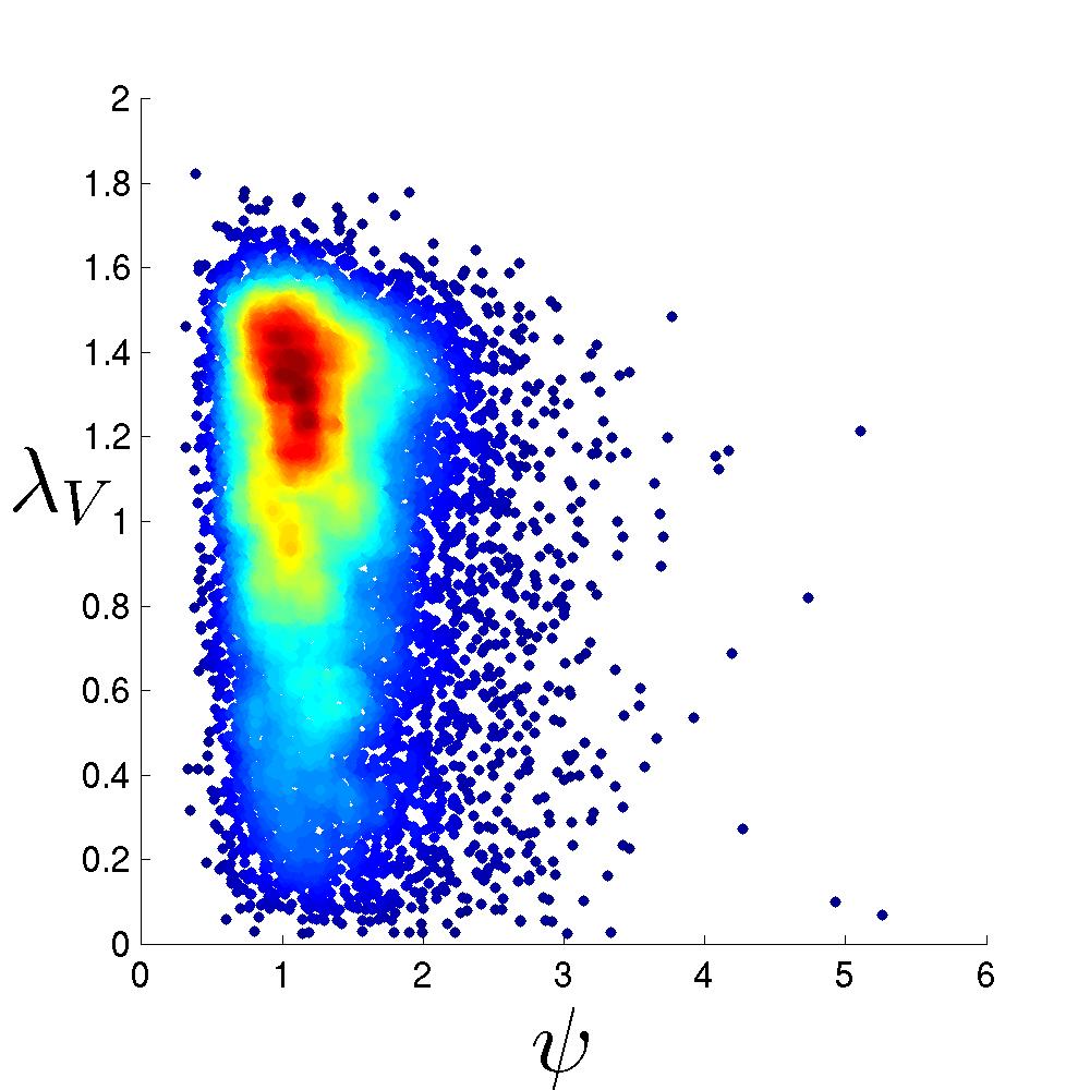
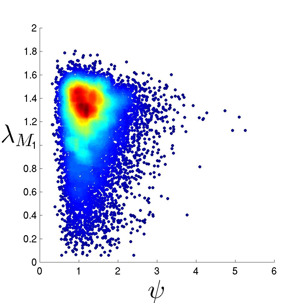
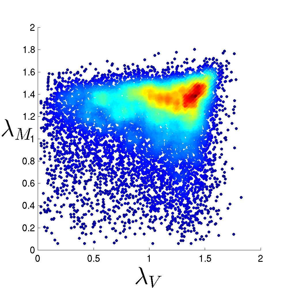
Figure 8: Macaque 400: bivariate posterior margins for the dimensionless model parameters as annotated.

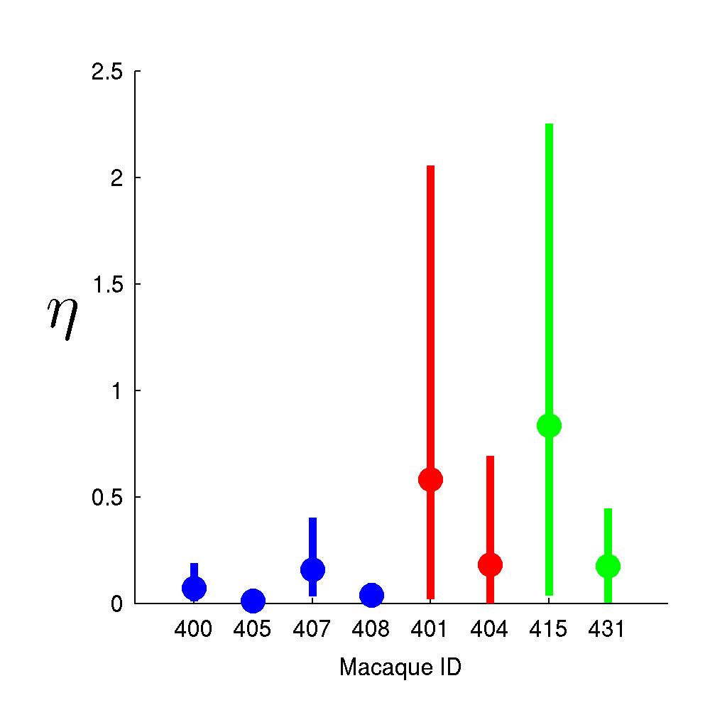
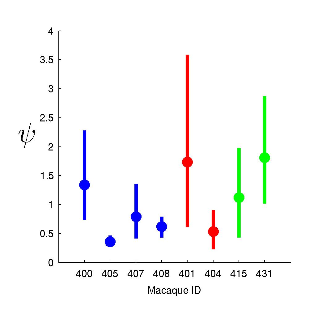
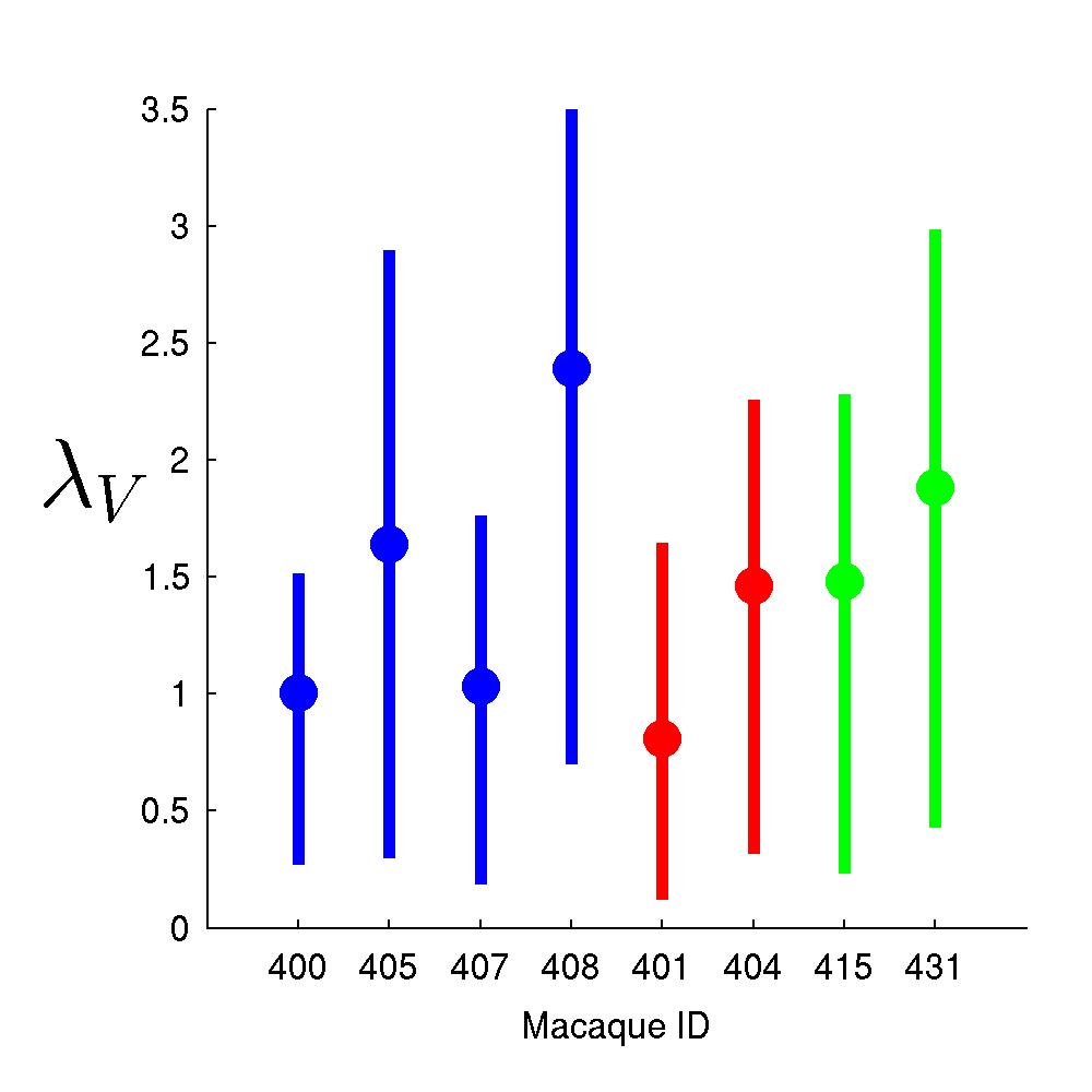
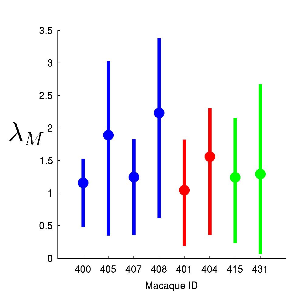
Figure 9: Marginal posterior means and 90% credible intervals for dimensionless model parameters on all 8 macaques. Color reflects vaccine immunization route: intra-nasal/intra-tracheal (blue), intra-rectal (red), intra-vagina (green).

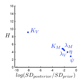
Figure 10: Macaque 400: Learnability summaries. Posterior:prior relative entropy $H$ against log of posterior to prior standard deviation, in some cases implicitly based on parameters following inverse c.d.f. transform to uniform priors as relevant.

6.8 Learnability of Model Parameters

To quantify and analyze the extent of learning about each parameter, we evaluate two indices based on the marginal posterior samples for each. The first index is the entropy ($H$) of the posterior relative to the prior, computed based on a binned representation of the posterior and prior distributions. The second index is the log ratio of marginal posterior to prior standard deviations. We transformed parameters having non-uniform priors (i.e., parameters $K_{V},K_{M},\eta,\psi,\lambda_{V},\lambda_{M})$ before computing these indices; the transformations were based on inverse prior cdfs so that the indices compare posteriors to uniform priors.

Figure 10 shows an illustrative example of these “learnability indices” for macaque #400; those for other macaques are comparable and can be found in the Supplementary material. There is limited data-based information about the three parameters $(V_{0},\tau_{M},\tau_{V}),$ very much more significant information about parameters $(\gamma,\delta,K_{V},\alpha,\rho),$ with the others in-between. There is similarly variation in the degrees of “learnability” of the dimensionless parameters, evident in Figure 10. While $\eta,\psi$ appear less learnable than others for macaque #400, their posterior SDs are smaller than prior SDs by at least a factor of 2, and in the case of $\eta$ it is almost a factor of 5, so that data information on these two parameters– earlier noted as reflecting substantial differences across macaques– is appreciable.

7 Additional Comments

The HIV/SIV immune vaccine study exemplifies emerging studies that aim to evaluate and compare efficacies of candidate vaccine designs in terms of resulting dynamic immune responses. As experimental techniques develop, we will see larger such experiments– in human subjects as well as NHPs– with time series data at a higher level of time resolution. The models developed here represent key aspects of progression of viral and memory cells, with time delays and stochastic elements that are evidently relevant. The constrained model form allows us to identify information in even this very sparse data about some of the model parameters, including differences across subjects in key rate $(\beta)$ and maximum level ($K_{V},K_{M})$ parameters that relate to critical aspects of the response profile. We also capture meaningful levels of between-subject variability that are likely to be even more relevant in future human studies.

Fitting non-linear dynamic models– with inherently long series of latent states to be inferred, along with multiple parameters– based on sparse time series data is an outstanding research challenge in computational statistics. After detailed development and evaluation of a range of MCMC and sequential Monte Carlo techniques, we have defined a direct coupling of analytic approximation-based MCMC with an ABC strategy that appears quite effective in Bayesian calibration of our model. Biases inherent in the MCMC analysis based on analytic approximations can be corrected by a second stage ABC processing of MCMC outputs, while cases with little or no bias remain relatively unchanged. Bayesian analysis naturally and gracefully handles the sparsity of data relative to a high-dimensional latent state and model parameters: posterior distributions appear similar to priors for parameters that are not learnable, while uncertainties in posteriors for other parameters and latent states capture and quantify the extent of information relevant to those aspects. Evidently, the overall strategy– though developed for this applied study– could be generalized in various ways as well as used directly in other applications of non-linear dynamic models.

The HIV/SIV vaccination study exhibits this selective learning about model parameters. Marginal posteriors for some parameters are highly concentrated relative to the priors, whereas for others the posterior is relatively similar to the prior. The inclusion of a time delay is a key model component, and all non-dimensional parameters are learnable. Interestingly, the results raise suggestions that the dynamics of the immune response depends on the vaccination route. This is not obvious from inspection of the time series data alone, and suggests follow-on experiments. With additional experimental data coming on stream, we are now in a position to address future analyses with perhaps more informative priors that build on the results here. One other area for further development is to consider hierarchical models that link parameters of models in a given immunization route group via a second stage prior, and even, perhaps, then add a further hierarchical component to link hyper-parameters across route groups. This would enable and encourage– when relevant– information sharing that could be beneficial, especially in contexts like this where data on each subject is sparse. Such developments, while beyond the scope of this paper, are under study.

Supplementary Material: Additional Figures

This supplement includes the additional graphical summaries of posteriors from the analysis of all 8 macaques, together with the raw time series data.

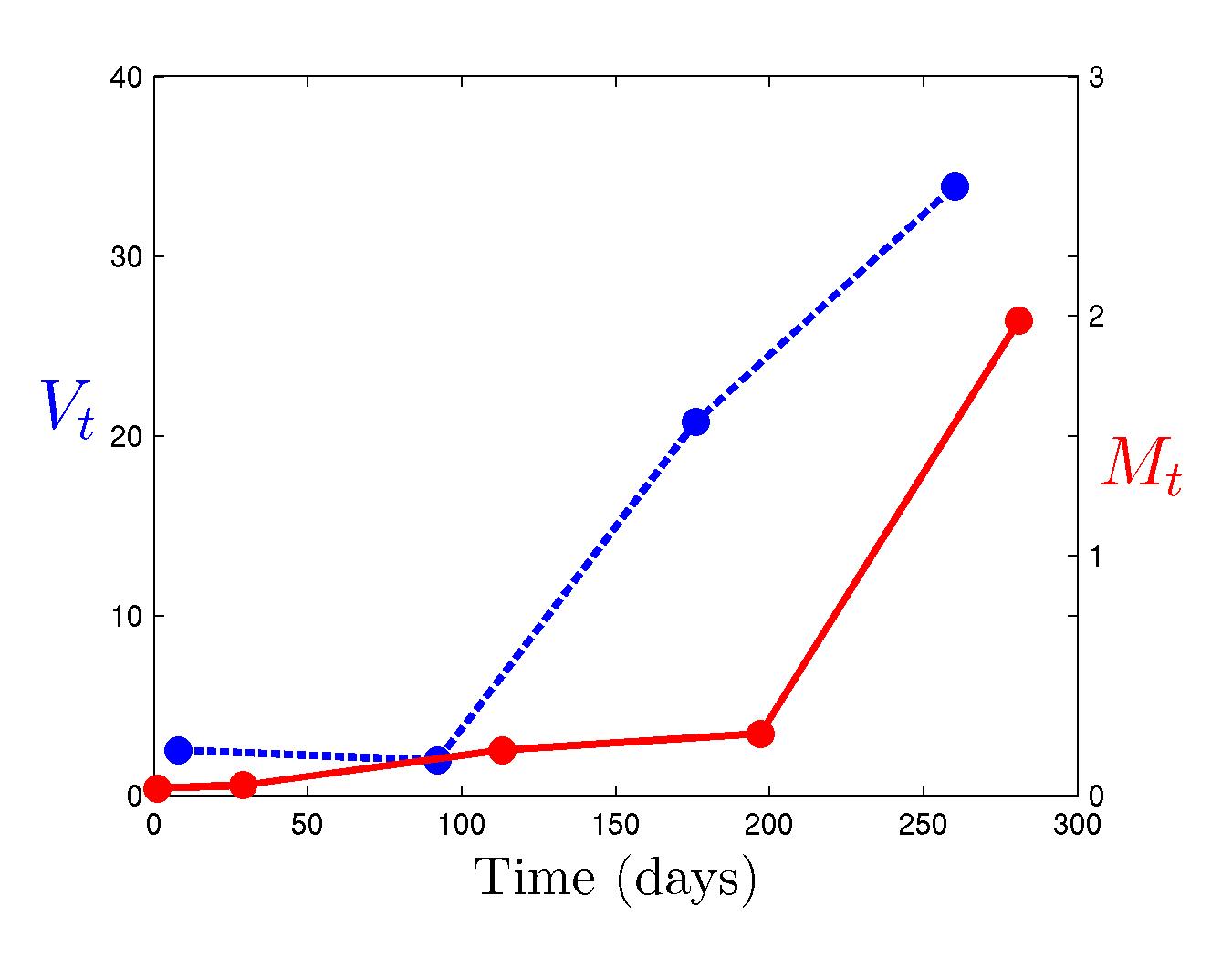
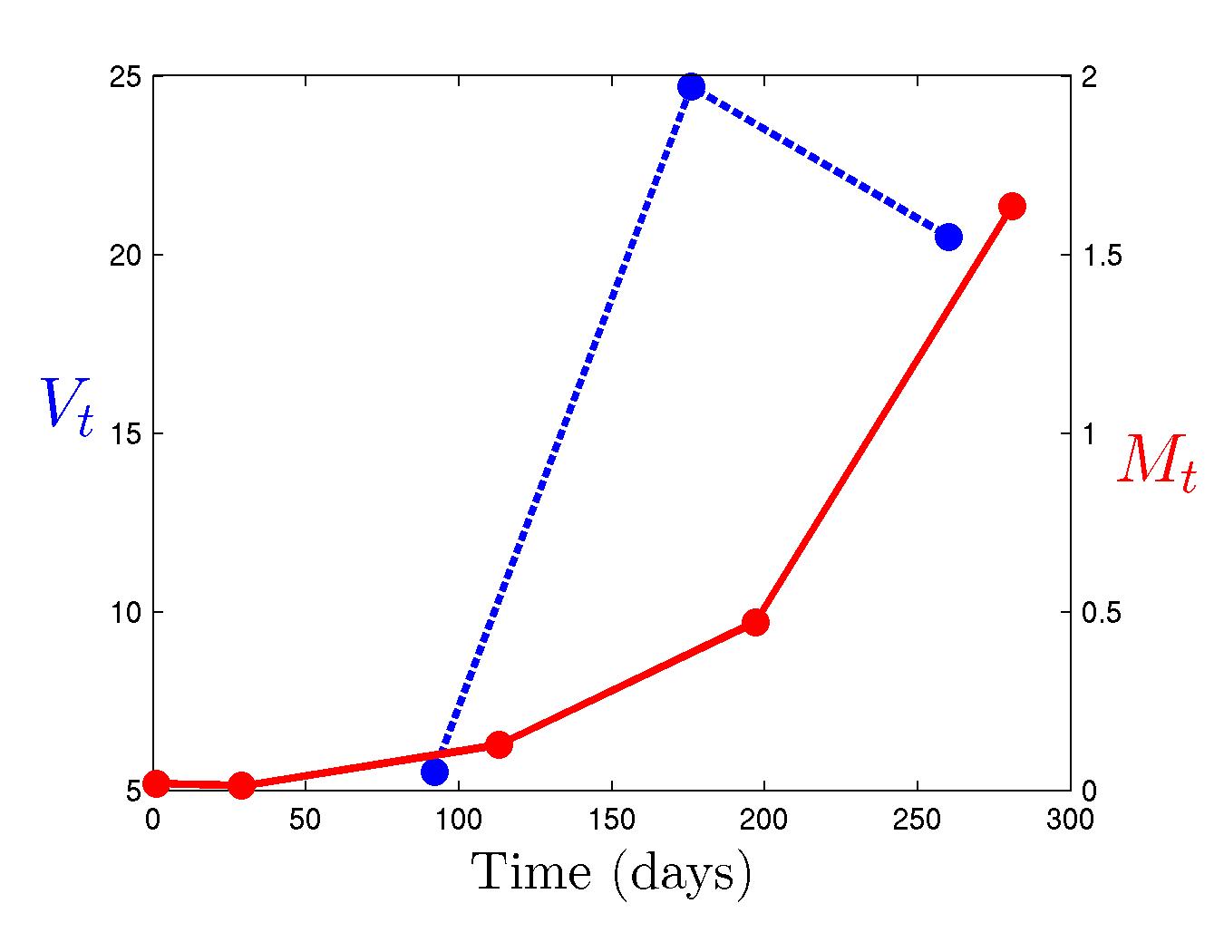
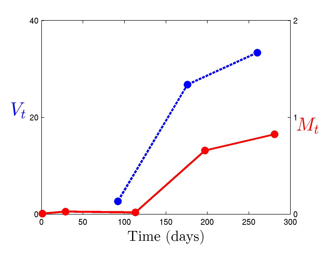
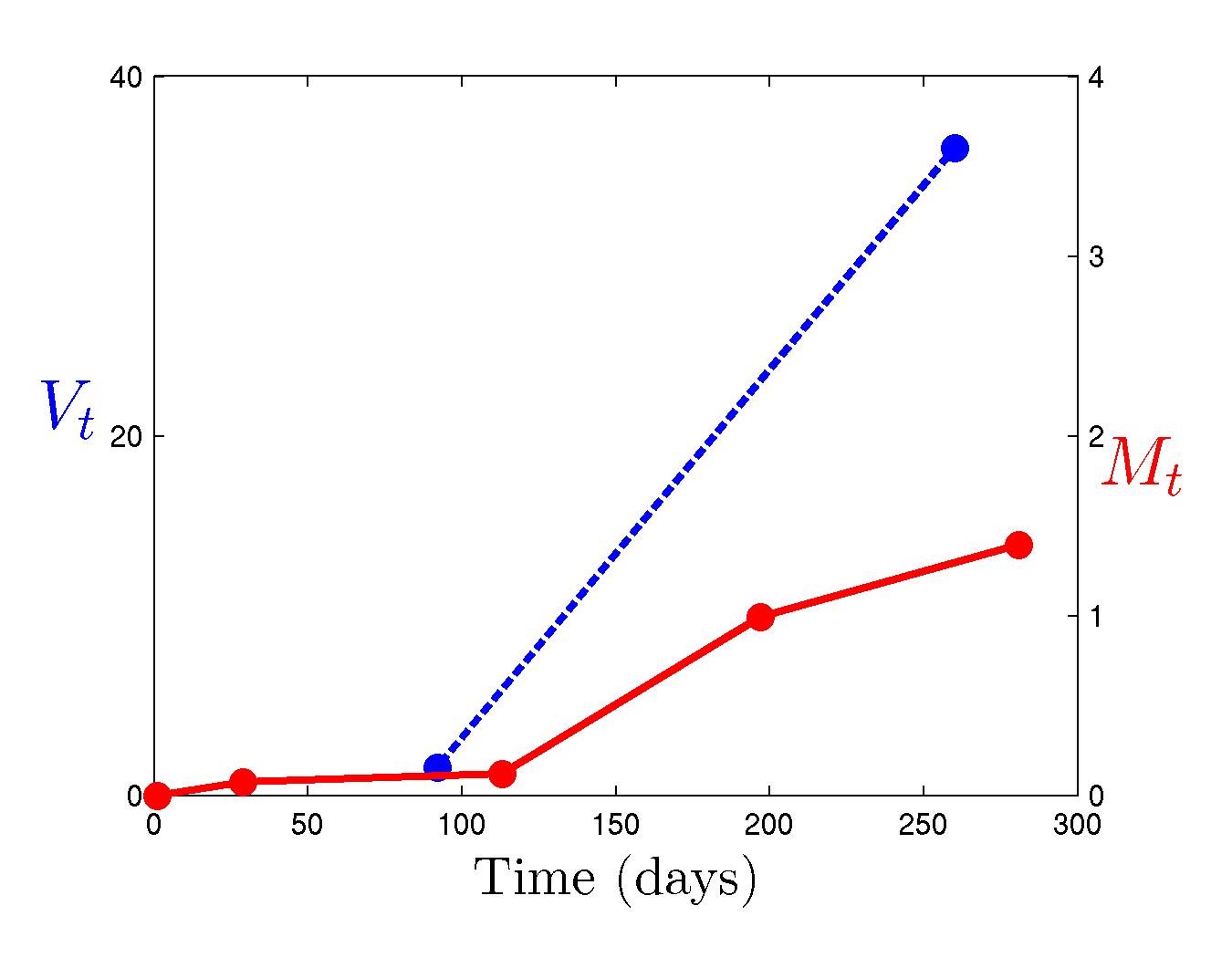
Figure 11: Observed data $V_{t}$ (blue) and $M_{t}$ (red) for all 8 macaques (subject IDs 400, 401, 404, 405, 407, 408, 415 and 431, respectively, from top left running left-to-right then down the rows).

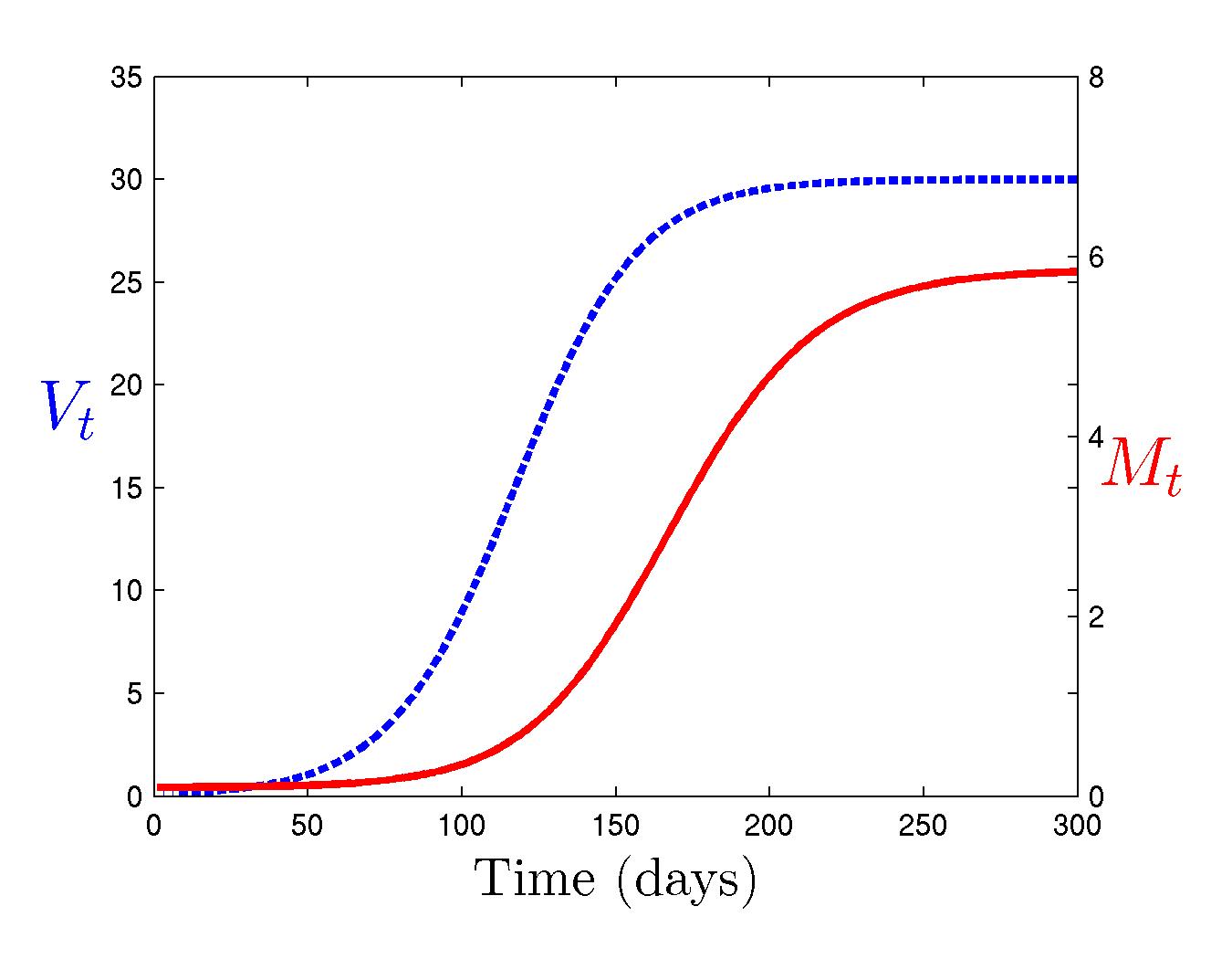
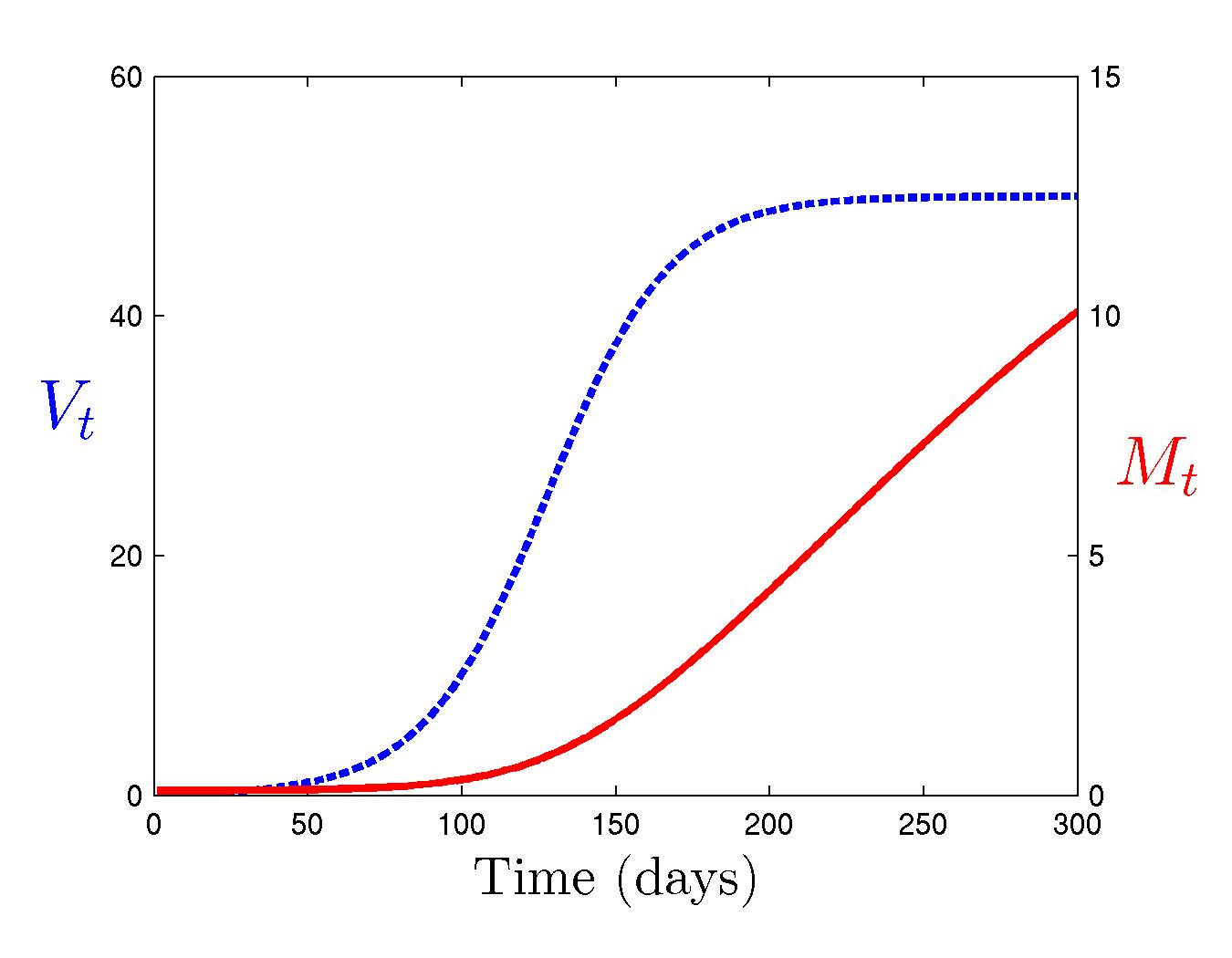
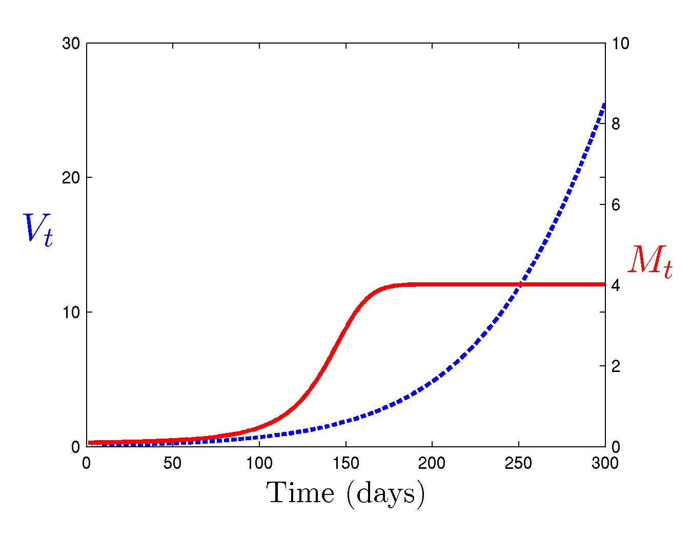
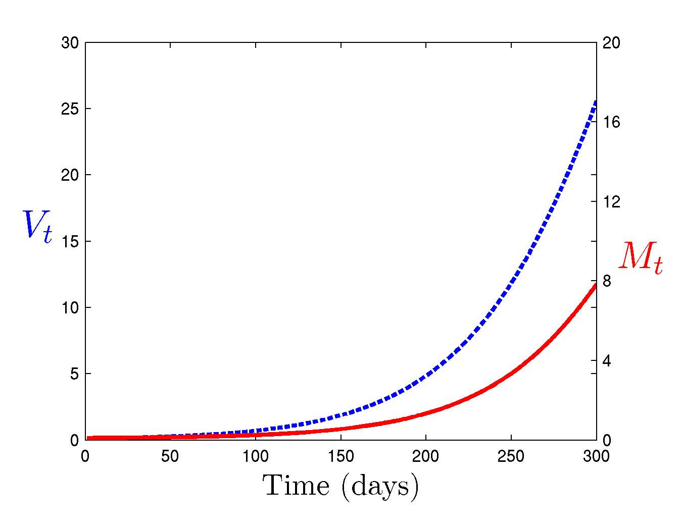
Figure 12: Synthetic trajectories of of $V_{t}$ (blue) and $M_{t}$ (red) from the initial ODE model based on forward integration, using $(V_{0},M_{0})=(0.5,0.5)$ as initial values. The four outcomes of the model are based on the parameters$\{\beta,K_{V},\alpha,\rho,K_{M}\}$ given by (0.05, 30, 0.001, 0.001, 5), (0.05, 50, 0.001, 0.0001, 10), (0.02, 80, 0.001, 0.05, 4), and (0.02, 80, 0.005, 0.0001, 6).

Figure 13: Synthetic trajectories of $V_{t}$ (blue) and $M_{t}$ (red) from the discrete-time, non-linear stochastic model with time delays. These start at $(V_{0},M_{0})=(0.5,0.5)$ and use model parameters chosen to be consistent with posteriors from the macaque study. The four outcomes (left to right, top down) are based on the parameters $\{\beta,\delta,\alpha,\rho,\gamma,\tau_{V},\tau_{M},\kappa^{2}_{V},\kappa^{2}_{M}\}$ given by (0.05, 0.05/30, 0.001, 0.001, 0.001/5, 5, 30, 0.025, 0.005), (0.05, 0.05/50, 0.001, 0.0001, 0.0001/10, 20, 5, 0.05, 0.01), (0.02, 0.02/80, 0.001, 0.05, 0.05/4, 10, 30, 0.1, 0.01), and (0.02, 0.02/80, 0.005, 0.0001, 0.0001/6, 20, 20, 0.2, 0.05).

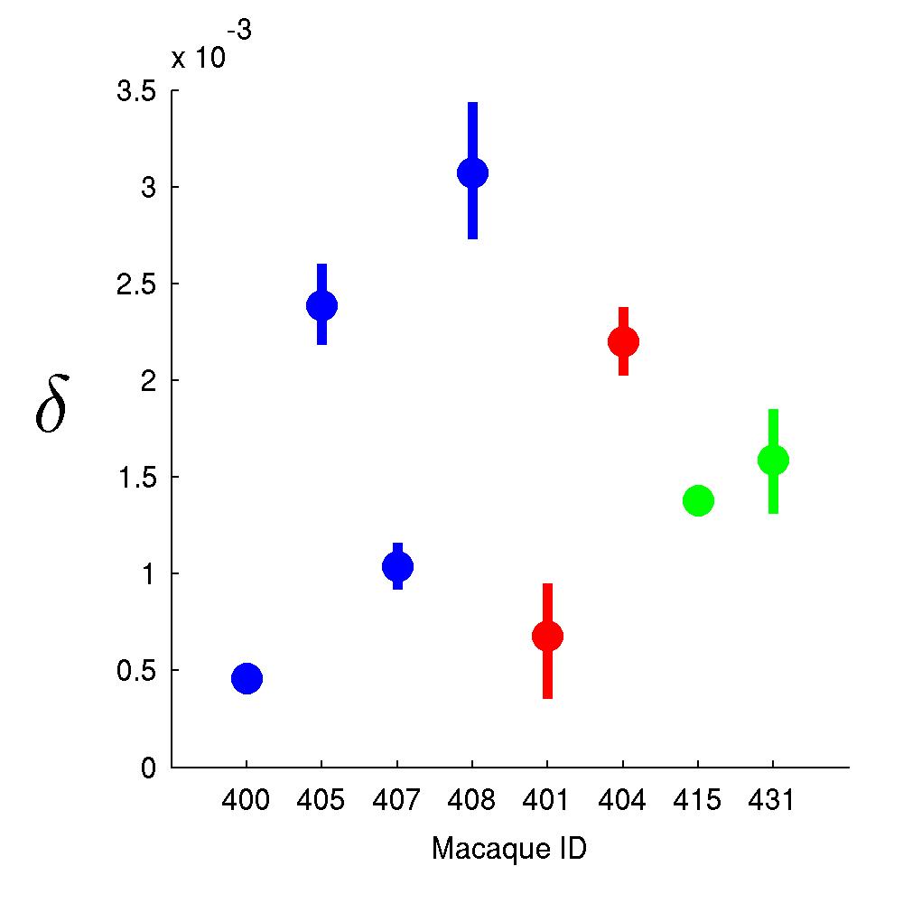
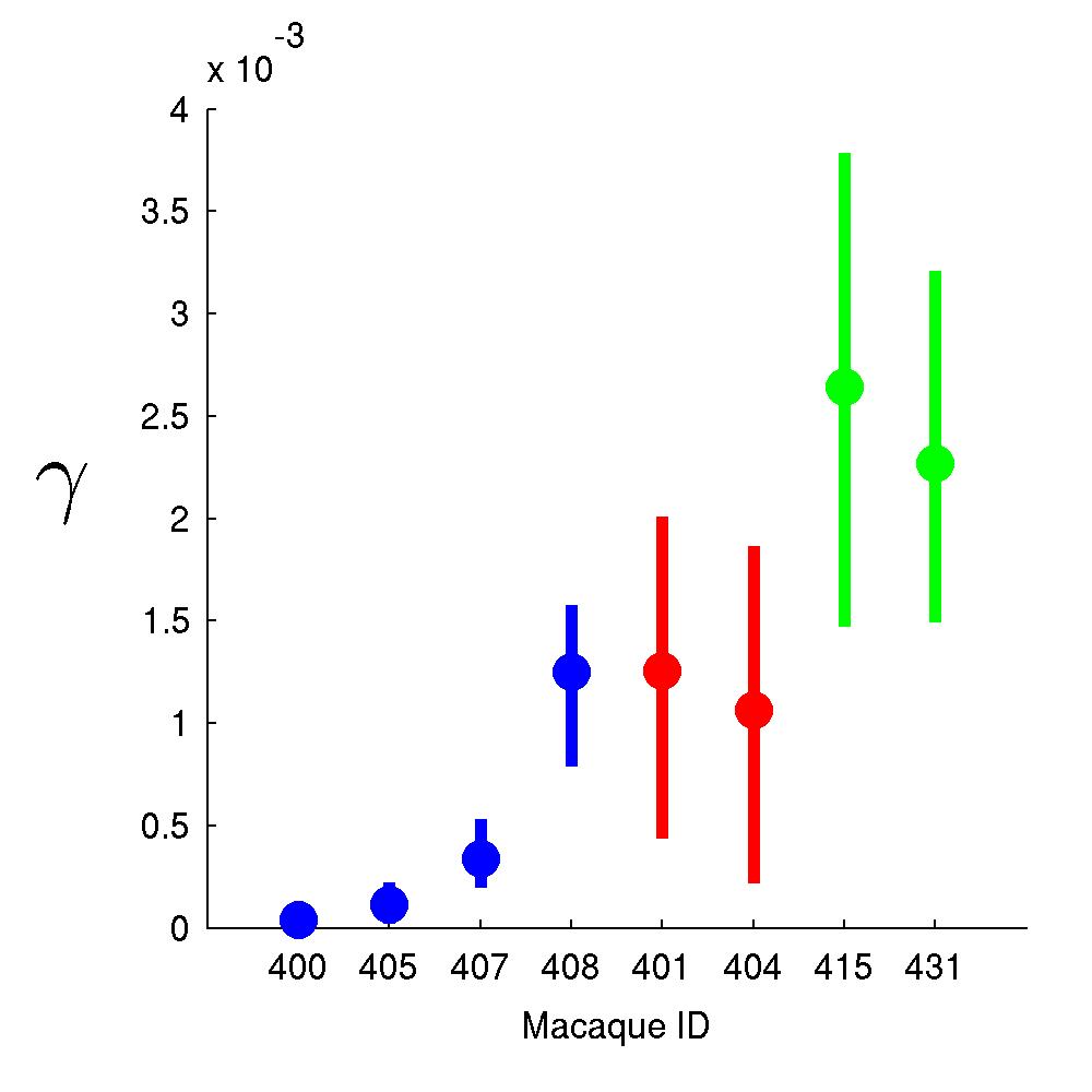
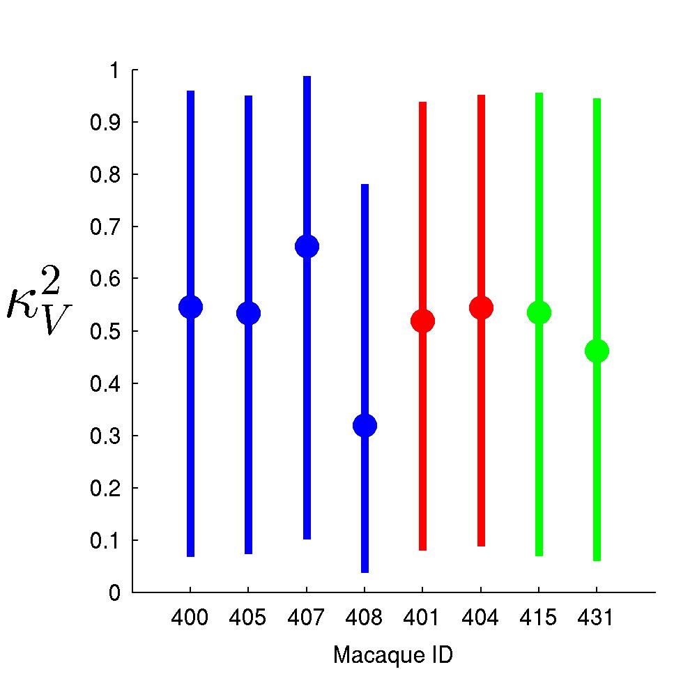
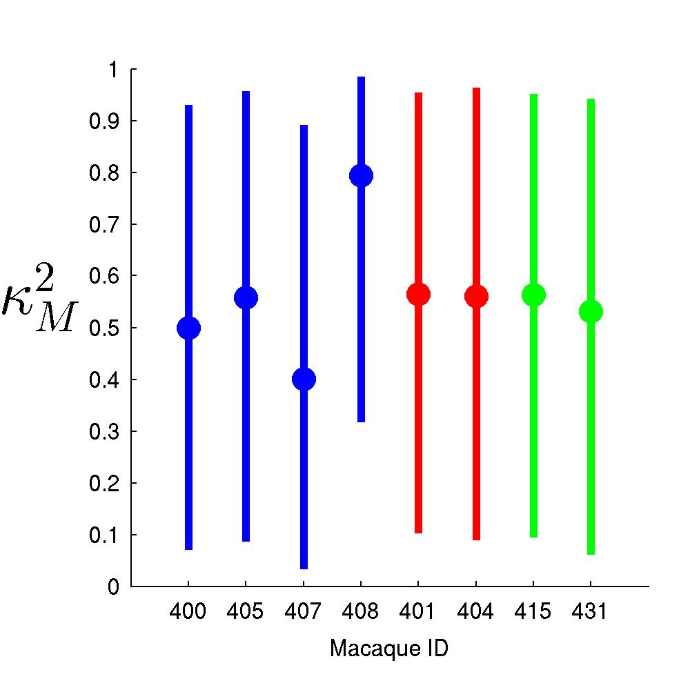
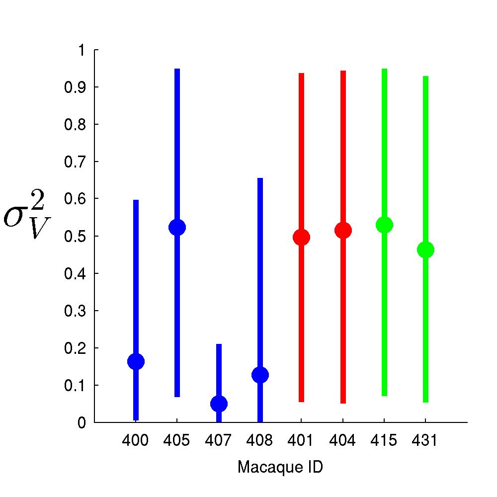
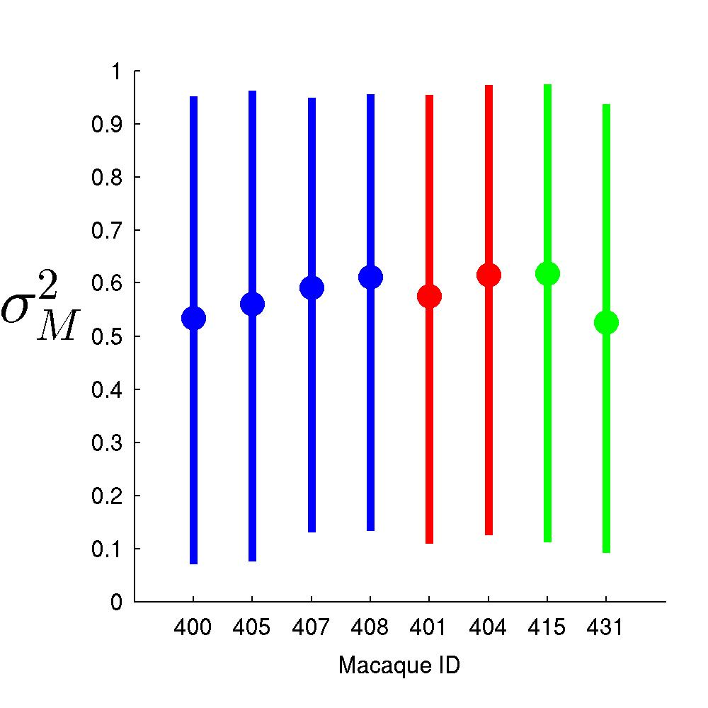
Figure 14: Marginal posterior means and 90% credible intervals for the full set of model parameters on all 8 macaques. Color reflects vaccine immunization route: intra-nasal/intra-tracheal (blue), intra-rectal (red), intra-vagina (green).

Figure 15: Posterior predictions for macaque #400: Top left: Observed data (blue); 50% (red), 95% (magenta) credible bands and median (gray) of posterior predictions for the latent states using only MCMC analysis. Top right: Same format, but based on MCMC+ABC analysis. Lower center: 100 sample trajectories from the posterior predictive distribution of the latent states from MCMC+ABC analysis.

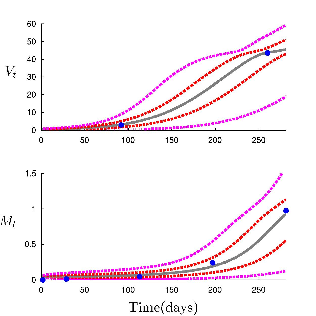
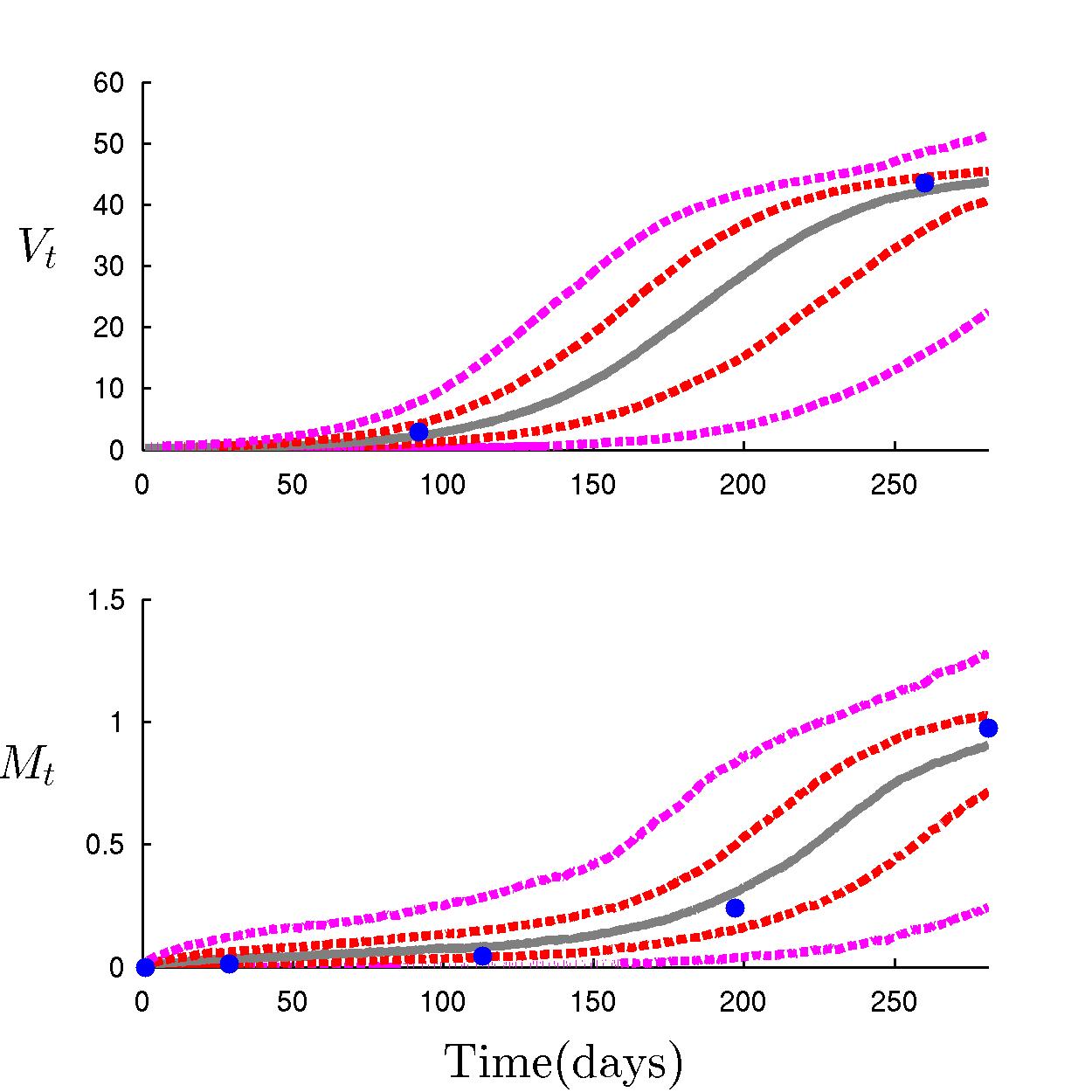
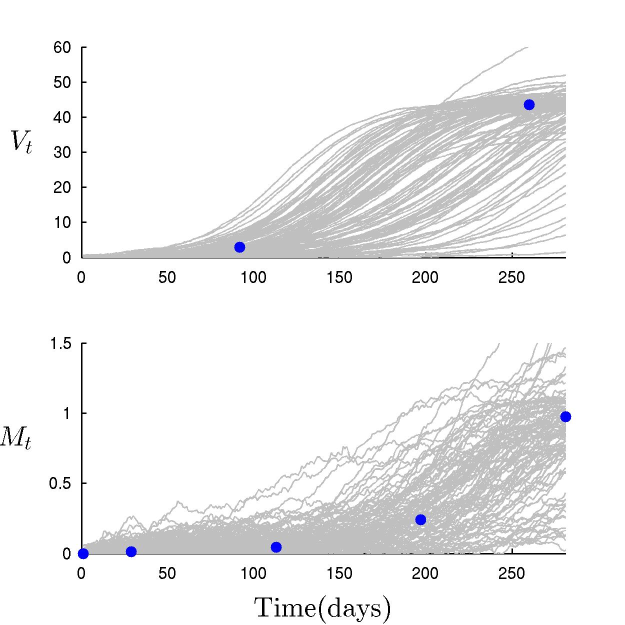
Figure 16: Posterior predictions for macaque #401: Top left: Observed data (blue); 50% (red), 95% (magenta) credible bands and median (gray) of posterior predictions for the latent states using only MCMC analysis. Top right: Same format, but based on MCMC+ABC analysis. Lower center: 100 sample trajectories from the posterior predictive distribution of the latent states from MCMC+ABC analysis.

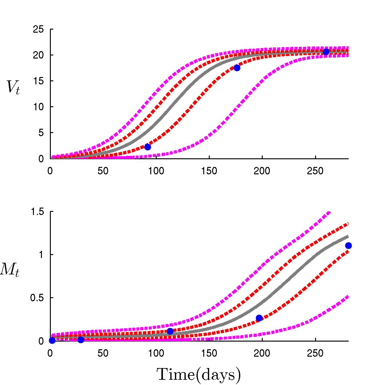
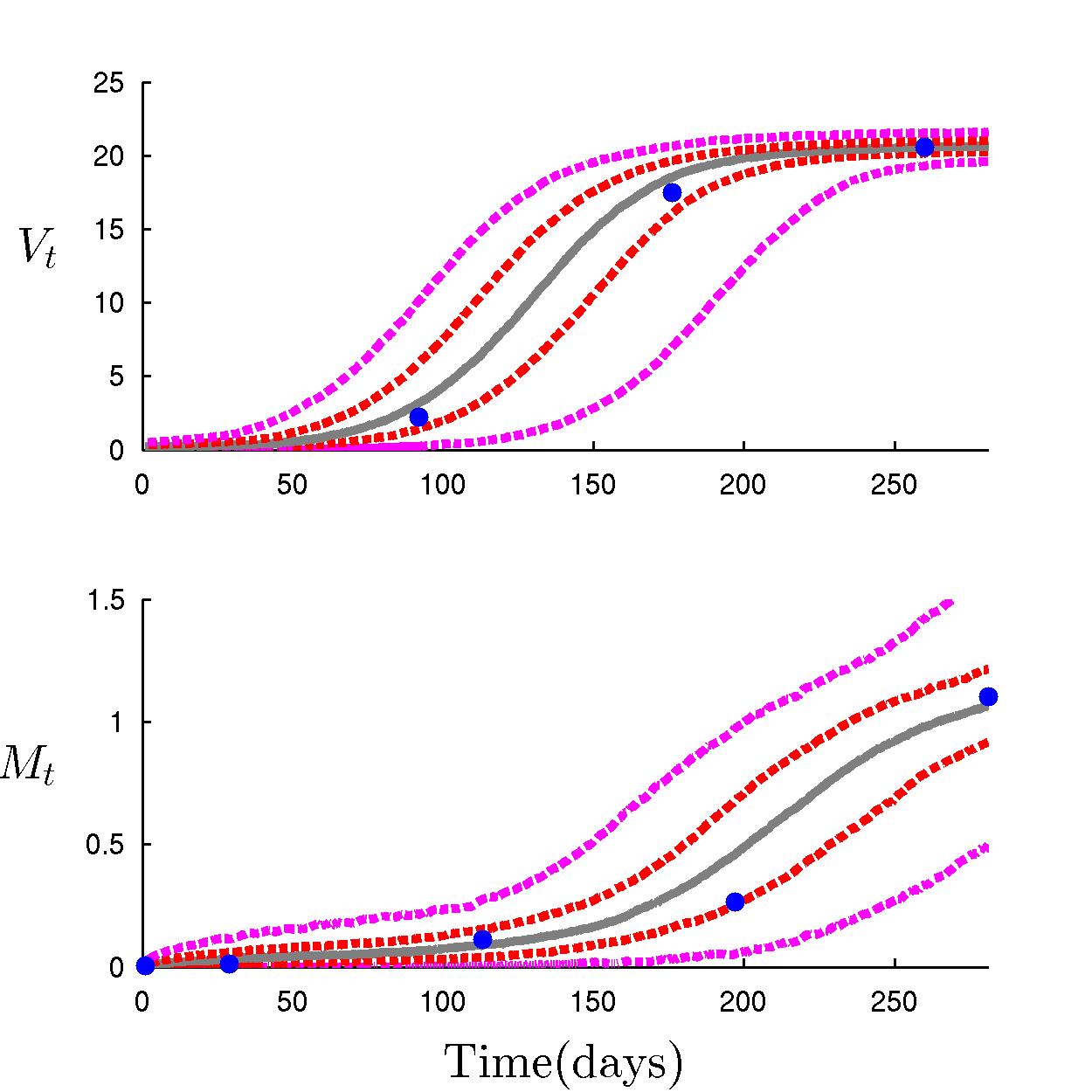
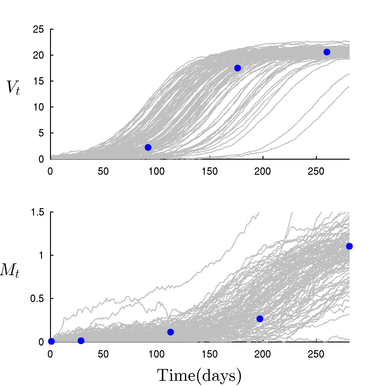
Figure 17: Posterior predictions for macaque #404: Top left: Observed data (blue); 50% (red), 95% (magenta) credible bands and median (gray) of posterior predictions for the latent states using only MCMC analysis. Top right: Same format, but based on MCMC+ABC analysis. Lower center: 100 sample trajectories from the posterior predictive distribution of the latent states from MCMC+ABC analysis.

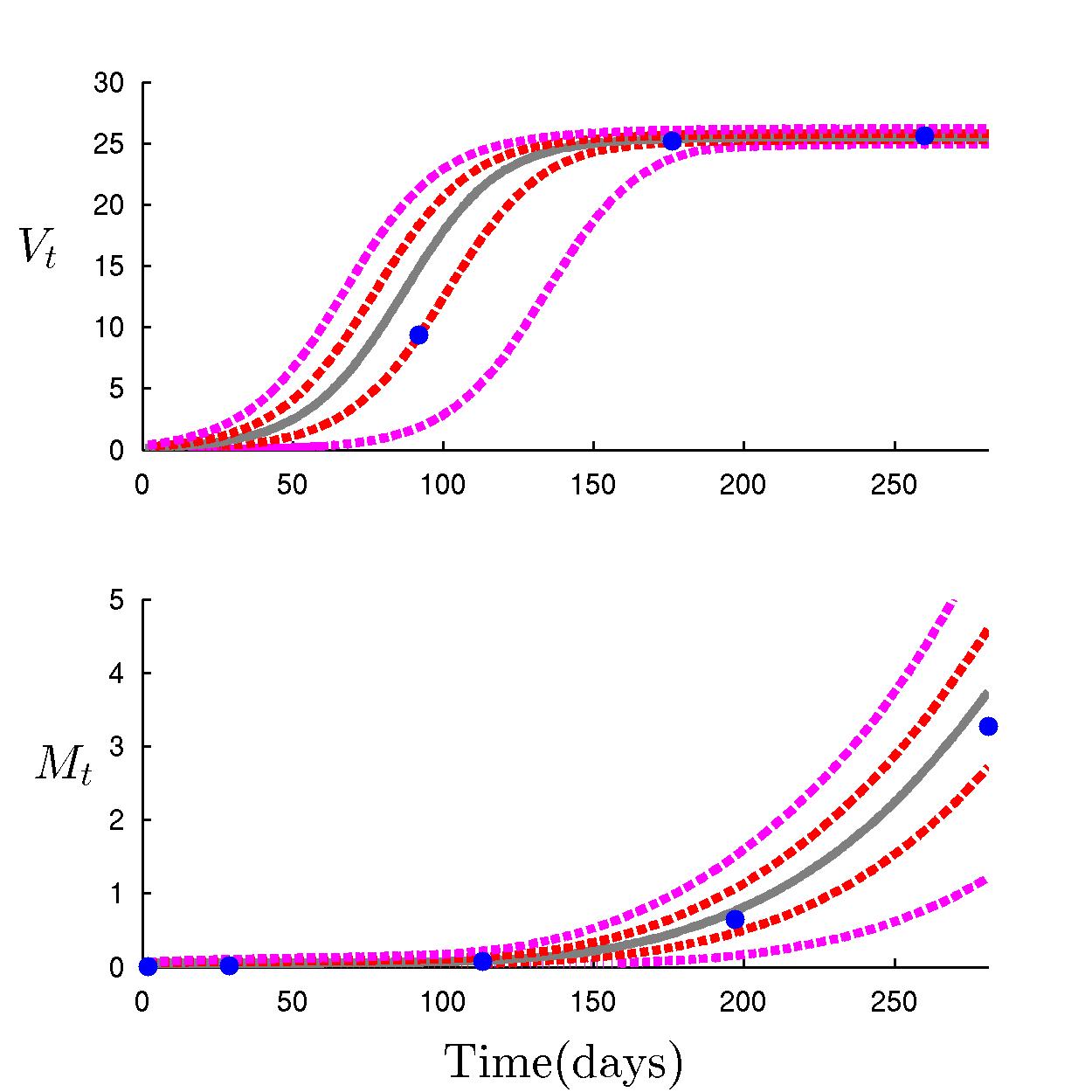
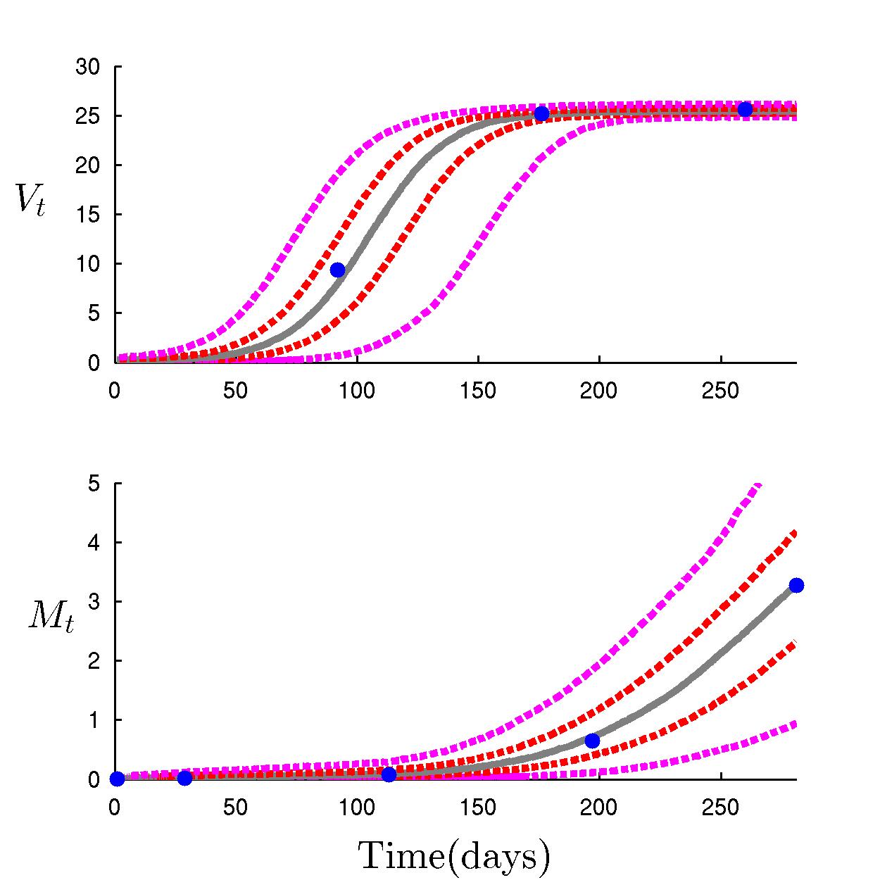
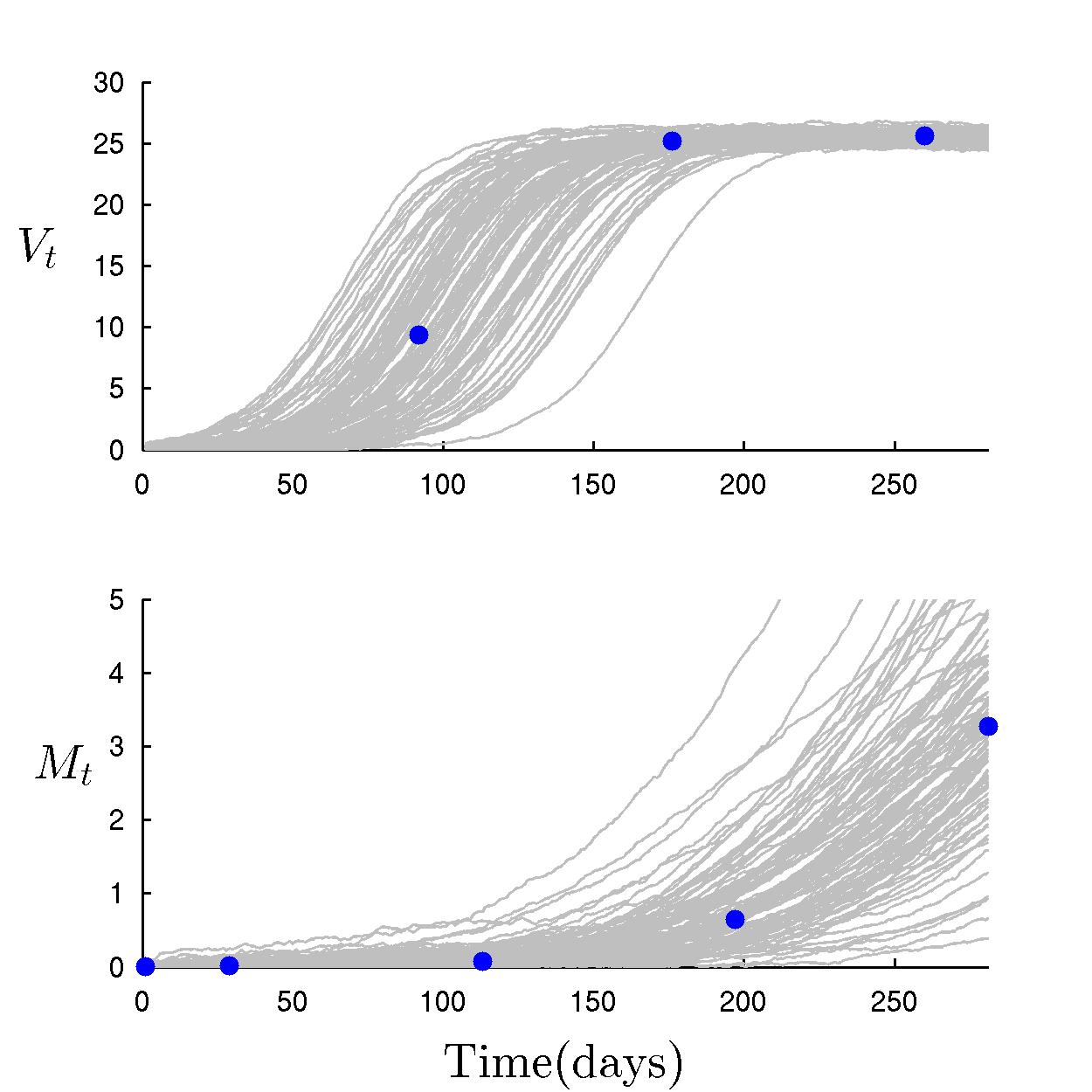
Figure 18: Posterior predictions for macaque #405: Top left: Observed data (blue); 50% (red), 95% (magenta) credible bands and median (gray) of posterior predictions for the latent states using only MCMC analysis. Top right: Same format, but based on MCMC+ABC analysis. Lower center: 100 sample trajectories from the posterior predictive distribution of the latent states from MCMC+ABC analysis.

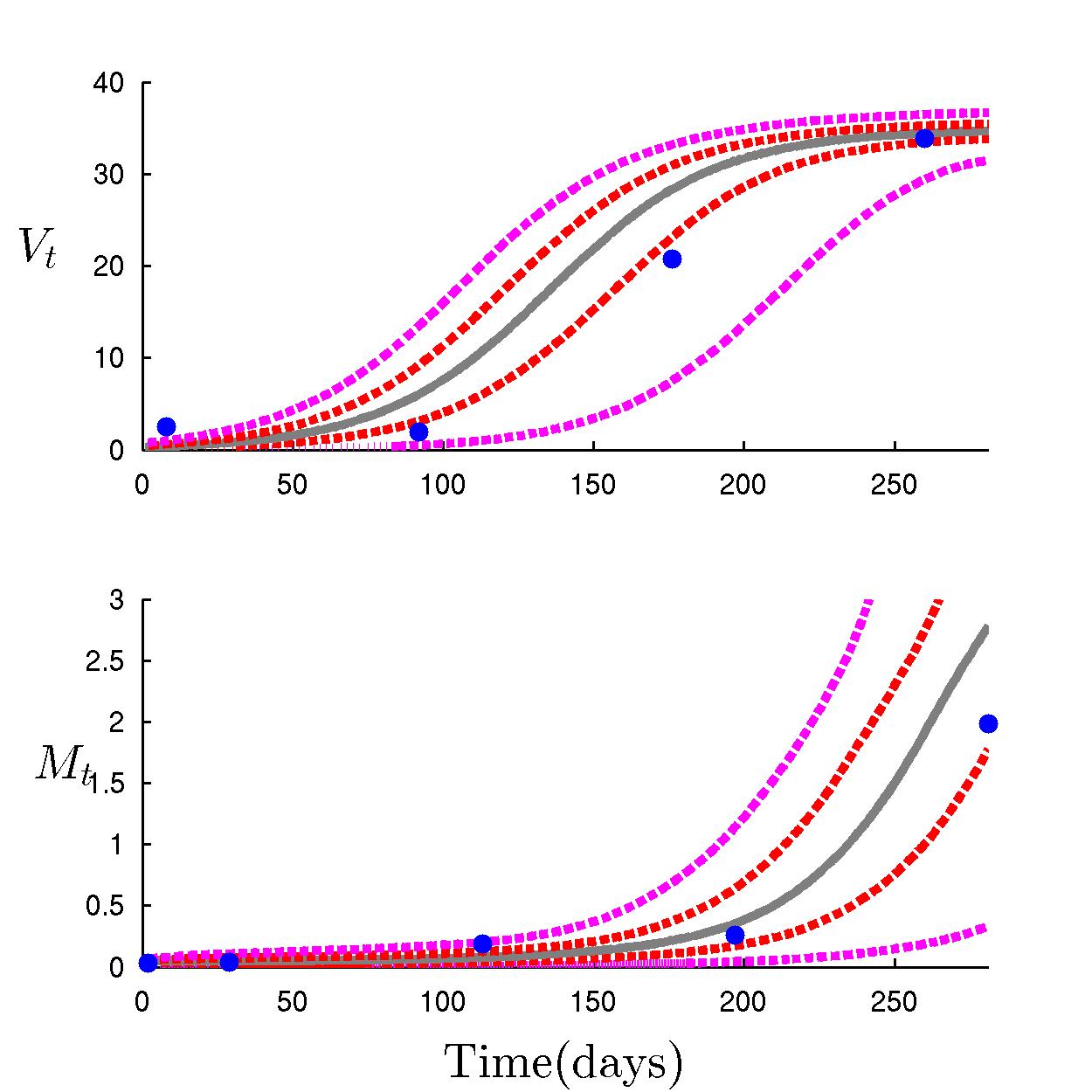
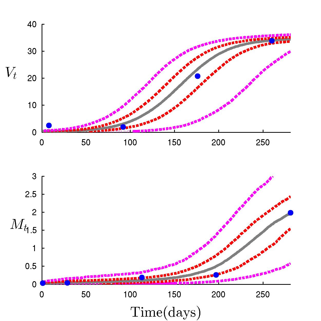
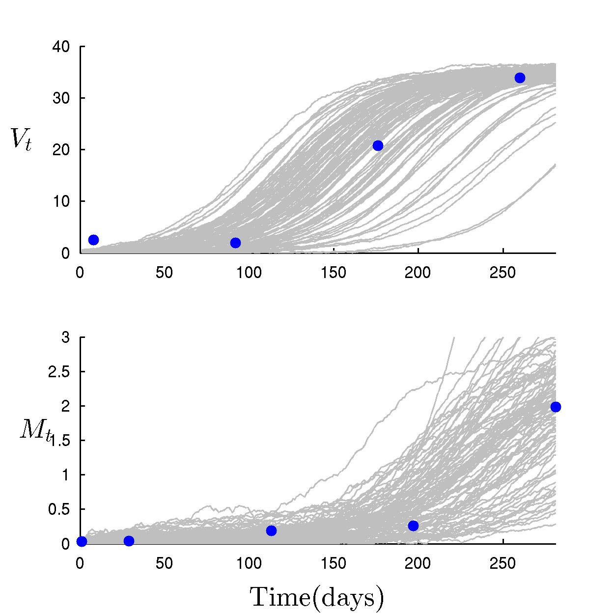
Figure 19: Posterior predictions for macaque #407: Top left: Observed data (blue); 50% (red), 95% (magenta) credible bands and median (gray) of posterior predictions for the latent states using only MCMC analysis. Top right: Same format, but based on MCMC+ABC analysis. Lower center: 100 sample trajectories from the posterior predictive distribution of the latent states from MCMC+ABC analysis.

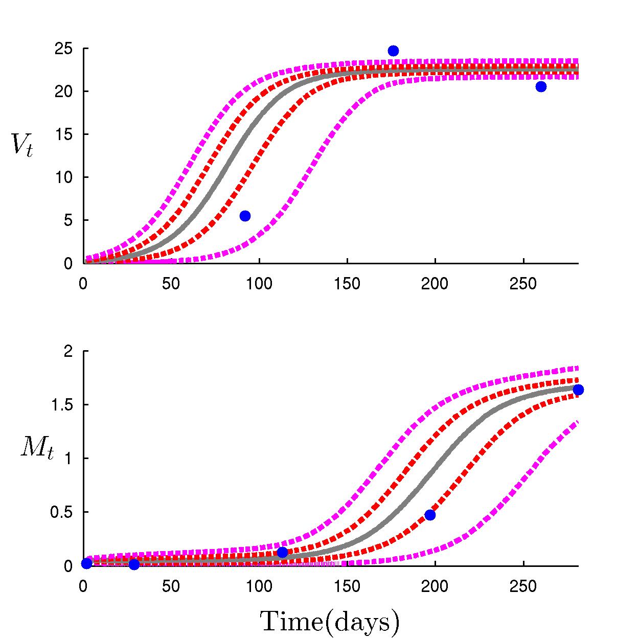
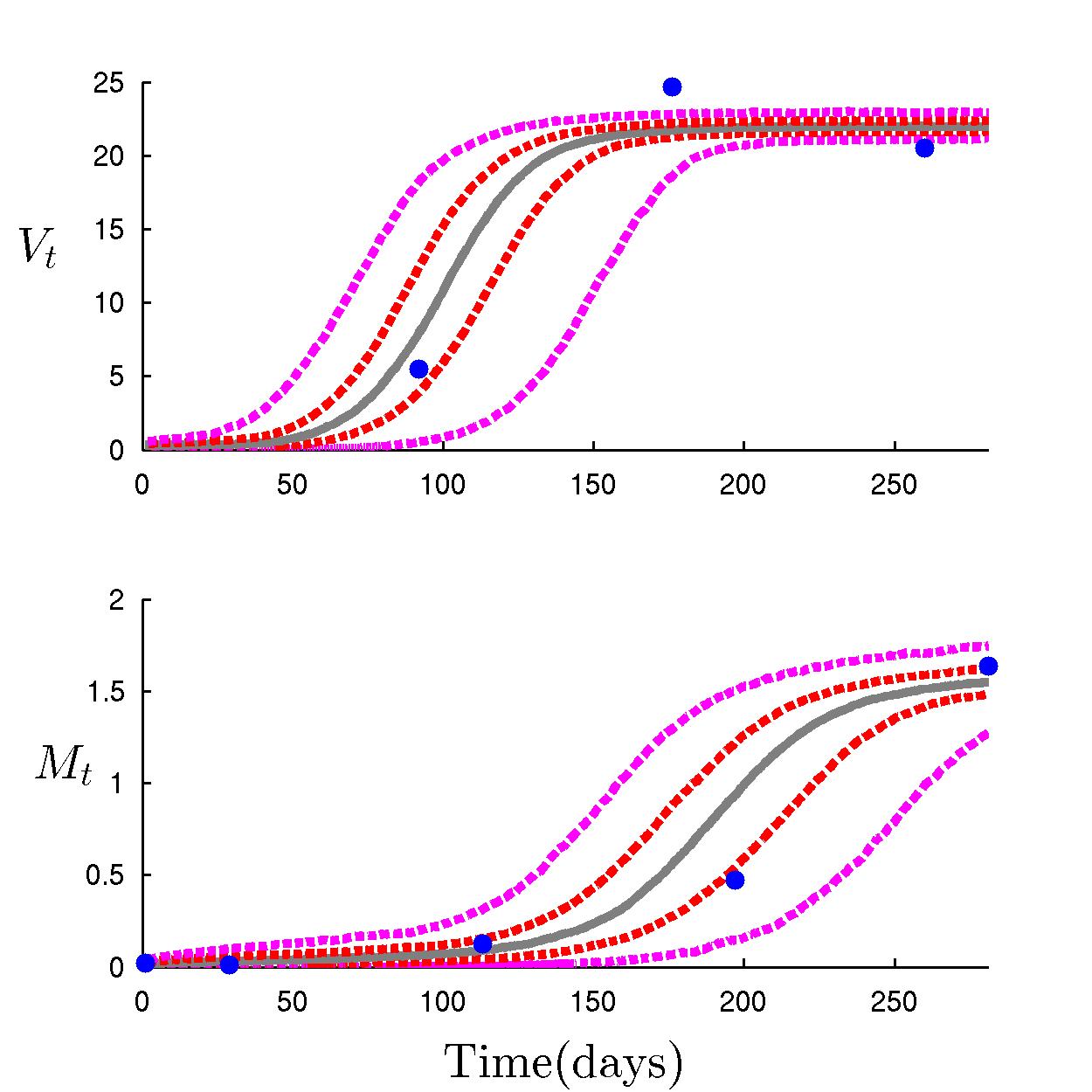
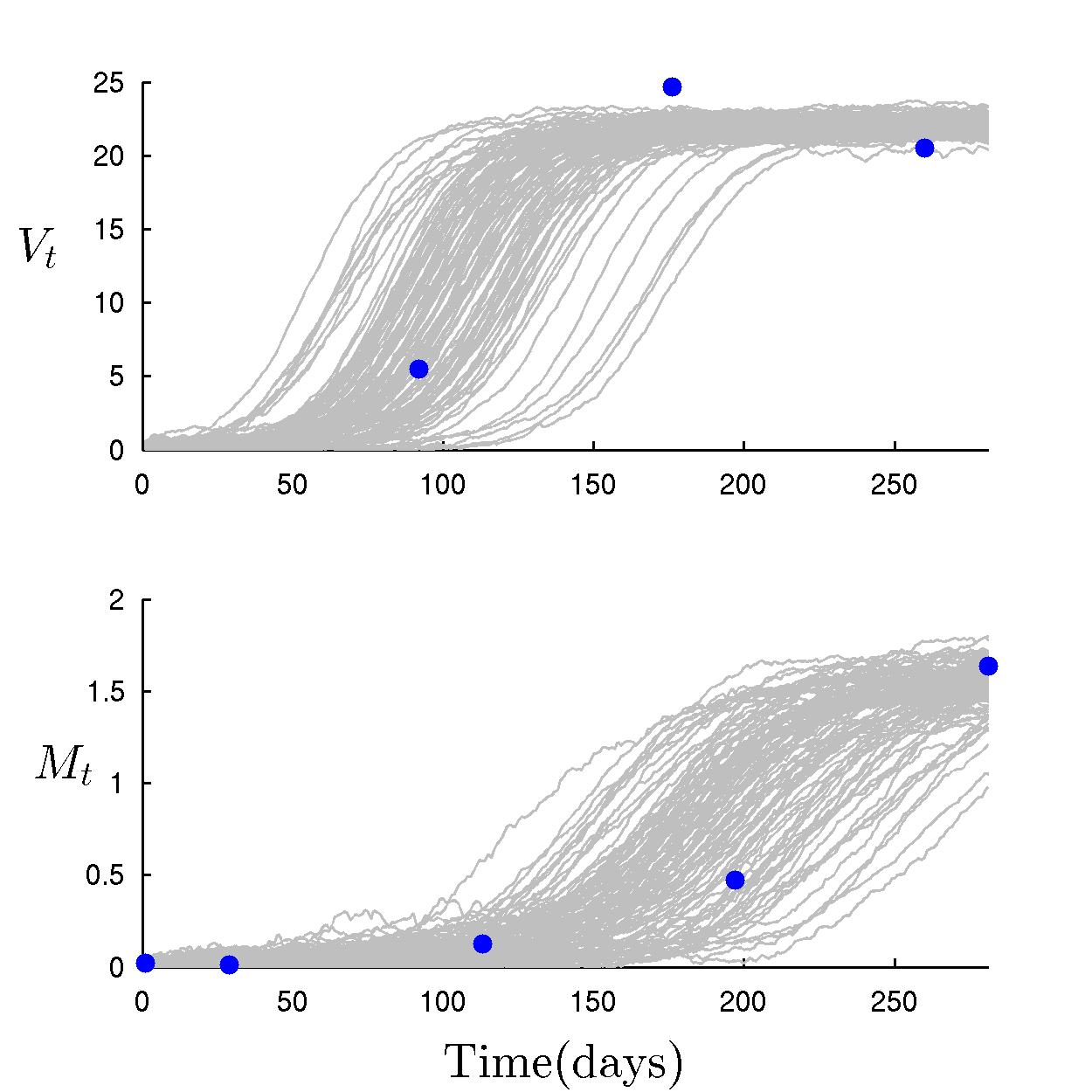
Figure 20: Posterior predictions for macaque #408: Top left: Observed data (blue); 50% (red), 95% (magenta) credible bands and median (gray) of posterior predictions for the latent states using only MCMC analysis. Top right: Same format, but based on MCMC+ABC analysis. Lower center: 100 sample trajectories from the posterior predictive distribution of the latent states from MCMC+ABC analysis.

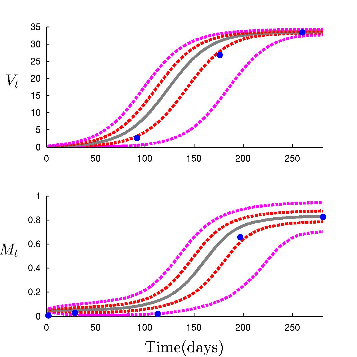
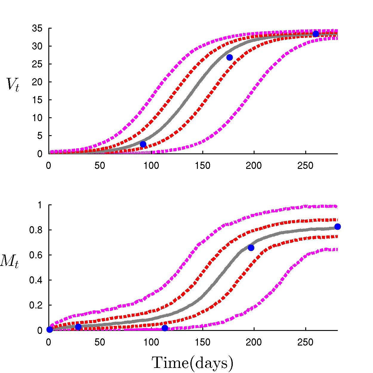
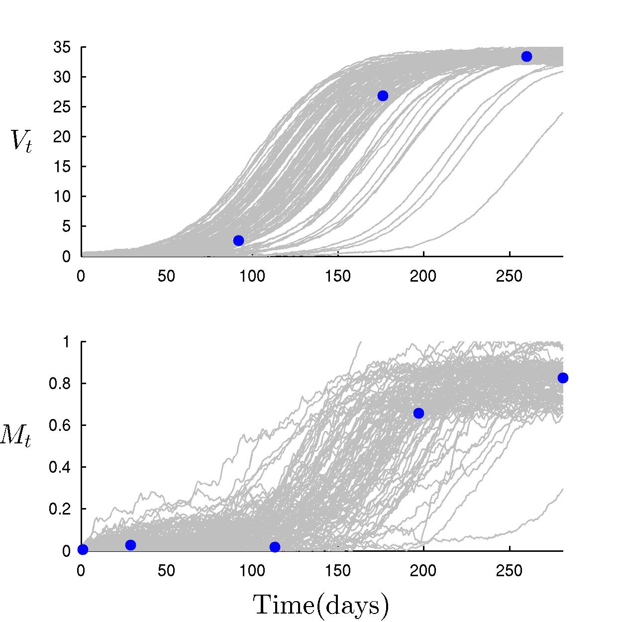
Figure 21: Posterior predictions for macaque #415: Top left: Observed data (blue); 50% (red), 95% (magenta) credible bands and median (gray) of posterior predictions for the latent states using only MCMC analysis. Top right: Same format, but based on MCMC+ABC analysis. Lower center: 100 sample trajectories from the posterior predictive distribution of the latent states from MCMC+ABC analysis.

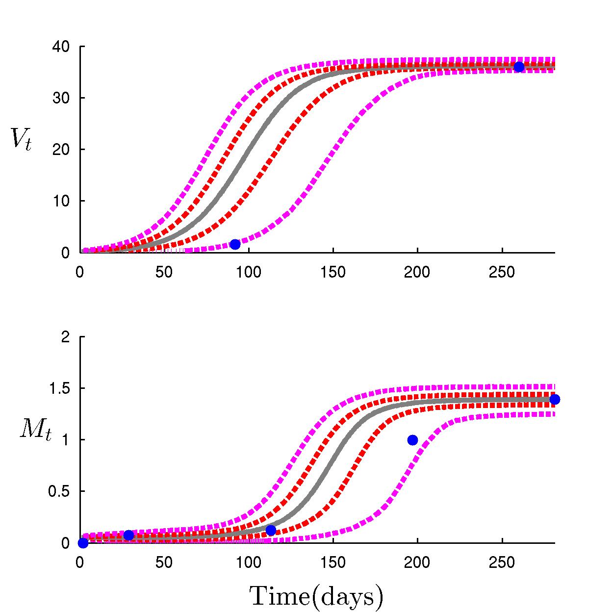
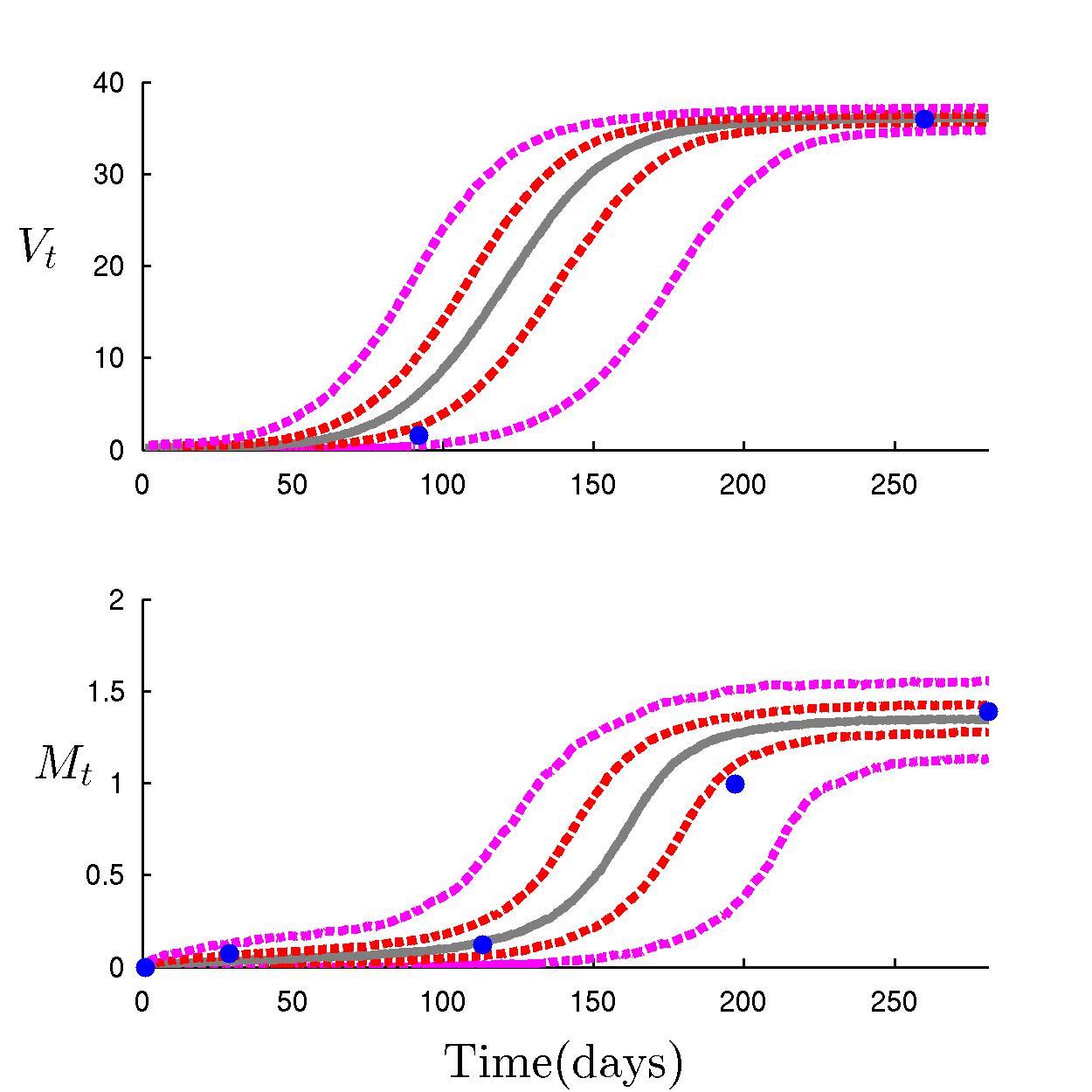
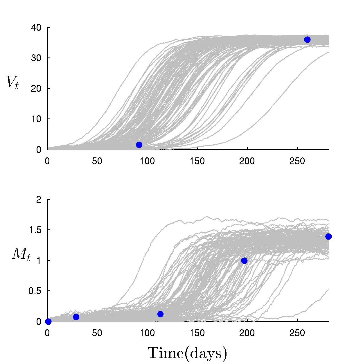
Figure 22: Posterior predictions for macaque #431: Top left: Observed data (blue); 50% (red), 95% (magenta) credible bands and median (gray) of posterior predictions for the latent states using only MCMC analysis. Top right: Same format, but based on MCMC+ABC analysis. Lower center: 100 sample trajectories from the posterior predictive distribution of the latent states from MCMC+ABC analysis.

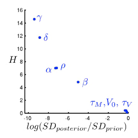
Figure 23: Macaque 400: Learnability summaries. Posterior:prior relative entropy $H$ against log of posterior to prior standard deviation, in some cases implicitly based on parameters following inverse c.d.f. transform to uniform priors as relevant.

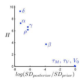
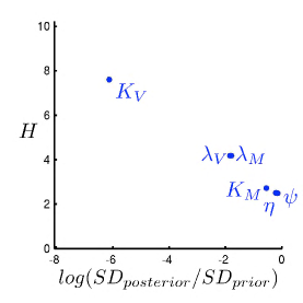
Figure 24: Macaque 400: Learnability summaries. Posterior:prior relative entropy $H$ against log of posterior to prior standard deviation, in some cases implicitly based on parameters following inverse c.d.f. transform to uniform priors as relevant.

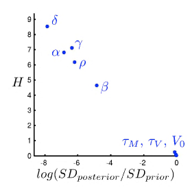
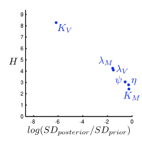
Figure 25: Macaque 404: Learnability summaries. Posterior:prior relative entropy $H$ against log of posterior to prior standard deviation, in some cases implicitly based on parameters following inverse c.d.f. transform to uniform priors as relevant.

Figure 26: Macaque 405: Learnability summaries. Posterior:prior relative entropy $H$ against log of posterior to prior standard deviation, in some cases implicitly based on parameters following inverse c.d.f. transform to uniform priors as relevant.

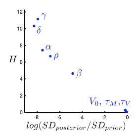
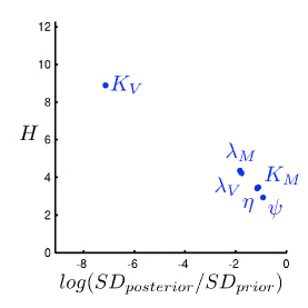
Figure 27: Macaque 407: Learnability summaries. Posterior:prior relative entropy $H$ against log of posterior to prior standard deviation, in some cases implicitly based on parameters following inverse c.d.f. transform to uniform priors as relevant.

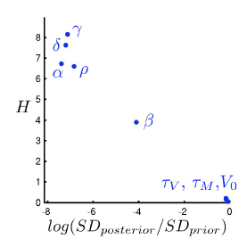
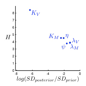
Figure 28: Macaque 408: Learnability summaries. Posterior:prior relative entropy $H$ against log of posterior to prior standard deviation, in some cases implicitly based on parameters following inverse c.d.f. transform to uniform priors as relevant.

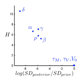
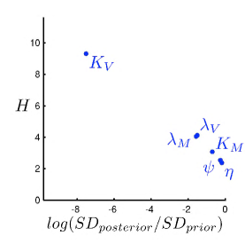
Figure 29: Macaque 415: Learnability summaries. Posterior:prior relative entropy $H$ against log of posterior to prior standard deviation, in some cases implicitly based on parameters following inverse c.d.f. transform to uniform priors as relevant.

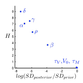
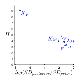
Figure 30: Macaque 431: Learnability summaries. Posterior:prior relative entropy $H$ against log of posterior to prior standard deviation, in some cases implicitly based on parameters following inverse c.d.f. transform to uniform priors as relevant.

References

- Beaumont et al. [2002] Beaumont, M., W. Zhang, and D. Balding (2002). Approximate Bayesian computation in population genetics. Genetics 162(4), 2025.
- Bonassi et al. [2011] Bonassi, F. V., L. You, and M. West (2011). Bayesian learning from marginal data in bionetwork models. Statistical Applications in Genetics & Molecular Biology 10, Art 49.
- Chan et al. [2008] Chan, C., F. Feng, J. Ottinger, D. Foster, M. West, and T. B. Kepler (2008). Statistical mixture modelling for cell subtype identification in flow cytometry. Cytometry, A 73(693-701), 693–701.
- Chan et al. [2010] Chan, C., L. Lin, J. Frelinger, V. Hebert, D. Gagnon, C. Landry, R. P. Sékaly, J. Enzor, J. Staats, K. J. Weinhold, M. Jaimes, and M. West (2010). Optimization of a highly standardized carboxyfluorescein succinimidyl ester flow cytometry panel and gating strategy design with discriminative information measure evaluation. Cytometry A 77, 1126–1136.
- De Boer [2007] De Boer, R. J. (2007, Mar). Understanding the failure of CD8+ T-cell vaccination against simian/human immunodeficiency virus. J. Virol. 81(6), 2838–2848.
- De Boer et al. [2003] De Boer, R. J., D. Homann, and A. S. Perelson (2003). Different dynamics of CD4+ and CD8+ T cell responses during and after acute lymphocytic choriomeningitis virus infection. The Journal of Immunology 171(8), 3928–3935.
- Drovandi and Pettitt [2011] Drovandi, C. C. and A. N. Pettitt (2011). Estimation of parameters for macroparasite population evolution using approximate bayesian computation. Biometrics 67(1), 225–233.
- Elemans et al. [2011] Elemans, M., N.-K. S. al Basatena, N. R. Klatt, C. Gkekas, G. Silvestri, and B. Asquith (2011). Why don’t cd8+ t cells reduce the lifespan of siv-infected cells in vivo? PLoS computational biology 7(9), e1002200.
- Evans and Silvestri [2013] Evans, D. T. and G. Silvestri (2013, Jul). Nonhuman primate models in AIDS research. Curr Opin HIV AIDS 8(4), 255–261.
- Golightly and Wilkinson [2011] Golightly, A. and D. J. Wilkinson (2011). Bayesian parameter inference for stochastic biochemical network models using particle Markov chain Monte Carlo. Interface Focus 1(6), 807–820.
- Johnston [2000] Johnston, M. I. (2000). The role of nonhuman primate models in aids vaccine development. Molecular Medicine Today 6(7), 267–270.
- Lin et al. [2013] Lin, L., C. Chan, S. R. Hadrup, T. M. Froesig, Q. Wang, and M. West (2013). Hierarchical Bayesian mixture modelling for antigen-specific T-cell subtyping in combinatorially encoded flow cytometry studies. Statistical Applications in Genetics and Molecular Biology 12, 309–331.
- Liu and West [2001] Liu, J. and M. West (2001). Combined parameter and state estimation in simulation-based filtering. In A. Doucet, J. D. Freitas, and N. Gordon (Eds.), Sequential Monte Carlo Methods in Practice, pp. 197–217. New York: Springer-Verlag.
- Morgan et al. [2008] Morgan, C., M. Marthas, C. Miller, A. Duerr, C. Cheng-Mayer, R. Desrosiers, J. Flores, N. Haigwood, S.-L. Hu, R. P. Johnson, et al. (2008). The use of nonhuman primate models in hiv vaccine development. PLoS medicine 5(8), e173.
- Niemi and West [2010] Niemi, J. B. and M. West (2010). Adaptive mixture modelling metropolis methods for Bayesian analysis of non-linear state-space models. Journal of Computational and Graphical Statistics 19, 260–280. PMC2887612.
- Patterson et al. [2012] Patterson, L. J., S. Kuate, M. Daltabuit-Test, Q. Li, P. Xiao, K. McKinnon, J. DiPasquale, A. Cristillo, D. Venzon, A. Haase, and M. Robert-Guroff (2012, May). Replicating adenovirus-simian immunodeficiency virus (SIV) vectors efficiently prime SIV-specific systemic and mucosal immune responses by targeting myeloid dendritic cells and persisting in rectal macrophages, regardless of immunization route. Clin. Vaccine Immunol. 19(5), 629–637.
- Patterson and Robert-Guroff [2008] Patterson, L. J. and M. Robert-Guroff (2008, Sep). Replicating adenovirus vector prime/protein boost strategies for HIV vaccine development. Expert Opin Biol Ther 8(9), 1347–1363.
- Prado and West [2010] Prado, R. and M. West (2010). Time Series: Modelling, Computation & Inference. Chapman & Hall/CRC Press.
- Pritchard et al. [1999] Pritchard, J., M. Seielstad, A. Perez-Lezaun, and M. Feldman (1999). Population growth of human Y chromosomes: a study of Y chromosome microsatellites. Molecular Biology and Evolution 16(12), 1791.
- Scherer and McLean [2002] Scherer, A. and A. McLean (2002). Mathematical models of vaccination. British Medical Bulletin 62(1), 187–199.
- Toni et al. [2009] Toni, T., D. Welch, N. Strelkowa, A. Ipsen, and M. Stumpf (2009). Approximate Bayesian computation scheme for parameter inference and model selection in dynamical systems. Journal of the Royal Society Interface 6(31), 187–202.
- West [1992] West, M. (1992). Modelling with mixtures (with discussion). In J. M. Bernardo, J. O. Berger, A. P. Dawid, and A. F. M. Smith (Eds.), Bayesian Statistics 4, pp. 503–524. Oxford University Press.
- West [1993a] West, M. (1993a). Approximating posterior distributions by mixtures. Journal of the Royal Statistical Society: Series B (Statistical Methology) 54, 553–568.
- West [1993b] West, M. (1993b). Mixture models, Monte Carlo, Bayesian updating and dynamic models. Computing Science and Statistics 24, 325–333.
- West and Harrison [1997] West, M. and P. J. Harrison (1997). Bayesian Forecasting & Dynamic Models (2nd ed.). Springer Verlag.
- Wilkinson [2006] Wilkinson, D. (2006). Stochastic Modelling for Systems Biology. London: Chapman & Hall/CRC.
- Wodarz [2008] Wodarz, D. (2008, Sep). Immunity and protection by live attenuated HIV/SIV vaccines. Virology 378(2), 299–305.