Reweighting QCD matrix-element and parton-shower calculations

Abstract

We present the implementation and validation of the techniques used to efficiently evaluate parametric and perturbative theoretical uncertainties in matrix-element plus parton-shower simulations within the Sherpa event-generator framework. By tracing the full $\alpha_{s}$ and PDF dependences, including the parton-shower component, as well as the fixed-order scale uncertainties, we compute variational event weights on-the-fly, thereby greatly reducing the computational costs to obtain theoretical-uncertainty estimates.
Keywords: QCD, NLO, Monte Carlo generators, Matrix Elements, Parton Showers

1 Introduction

The first operational run of the LHC collider during the years 2009-2013 was a tremendous success, clearly culminating in the announcement of the discovery of a Higgs-boson candidate by the ATLAS and CMS collaborations in July 2012 [1, 2]. Through a large number of experimental analyses, focusing on a variety of final states and observables, the LHC experiments (re)established and underpinned to an unprecedented level of accuracy the validity of the Standard Model of particle physics (SM) [3].

When comparing theoretical predictions with actual collider data, Monte-Carlo event generators prove to be an indispensable tool. In particular parton-shower Monte-Carlo programmes like Herwig [4, 5], Pythia [6] and Sherpa [7, 8] provide simulations at the level of exclusive particle-level final states [9]. The cornerstones of these generators are their implementations of QCD parton-shower algorithms and their modelling of the non-perturbative parton-to-hadron fragmentation process. With the advent of sophisticated techniques to combine parton-shower simulations with exact higher-order QCD calculations at leading [10, 11], next-to-leading [12, 13] and even next-to-next-to-leading order [14, 15, 16, 17], Monte-Carlo simulations have developed into high-precision tools, encapsulating the best of our current knowledge of perturbative QCD.

With these simulations being widely used for making SM predictions, e.g. of the background expectation in searches for New Physics or the detailed properties of Higgs-boson production final states, a comprehensive and efficient evaluation of associated theoretical uncertainties is of utmost importance. A comprehensive list of sources for generator uncertainties has been quoted in [18]. Following the categories identified there, when focusing on systematics related to the perturbative phases of event evolution, the following uncertainties might be distinguished:

• Parametric uncertainties reflecting the dependence of the prediction on input parameters such as couplings, particle masses or the parton-density functions (PDFs).

• Perturbative uncertainties originating from the fact that perturbation theory is used in making predictions, to fixed-order in the matrix elements and resummed to all-orders with a certain logarithmic accuracy in the showers, thereby, however, neglecting higher-order contributions. Similarly, the use of the large-$N_{c}$ approximation in the showers belongs in this category.

• Algorithmic uncertainties corresponding to the actual choices made in the implementation of the shower algorithm, i.e. for the evolution variable, the inclusion of non-singular terms in the splitting functions, or the employed matching/merging prescription. Per construction, for sensible choices, these systematics also correspond to higher-order perturbative corrections, but might be addressed separately.

In addition to the listed categories, generically non-perturbative effects such as hadronisation or the underlying event are described through phenomenological models that feature various generator-specific choices and parameters, typically subject to tuning against experimental data, see for instance [19, 20].

This publication focuses on the efficient evaluation of parametric and (some) perturbative uncertainties in matrix-element plus parton-shower simulations within the Sherpa event-generator framework. We present a comprehensive approach to fully trace the $\alpha_{s}$ and PDF dependences in the matrix-element and parton-shower components of particle-level Sherpa simulations in leading- [21] and next-to-leading [22] order merged calculations based on the Sherpa dipole-shower implementation [23]. Furthermore, we provide the means to quickly evaluate the renormalisation- and factorisation-scale dependence of the fixed-order matrix-element contributions. Our approach is based on event-wise reweighting and allows us to provide with a single generator run a set of variational event weights corresponding to the predefined parameter and scale variations, that would otherwise have to be determined through dedicated re-evaluations. The alternative event weights can either be accessed through the output of a HepMC event record [24], or directly passed via the internal interface of Sherpa to the Rivet analysis framework [25].

The systematics of leading-order parton-shower simulations with Herwig 7 have recently been discussed in [18], a corresponding reweighting procedure has been presented in [26]. A similar reweighting implementation for the Pythia 8 parton shower has also appeared recently [27]. A discussion of uncertainty estimates for the Vincia shower model can be found in [28, 29, 30]. A comprehensive comparison of various generators is presented in [31]. The impact of PDFs in parton-shower simulations has been discussed in [32, 33].

Our paper is organised as follows. In Sec. 2 we review the dependence structure of leading-order (LO) and next-to-leading-order QCD calculations on $\alpha_{s}$, the PDFs and the renormalisation and factorisation scales, and introduce the reweighting approach. In Sec. 3 we extend this to parton-shower simulations and in particular the algorithm employed in the Sherpa framework. In Sec. 4 we present the generalisation of the reweighting approach to multijet-merged calculations, based on leading and next-to-leading-order matrix elements matched to the parton shower. Our conclusions are summarised in Sec. 6. In App. A we present CPU time measurements that assess the reduction in computational time when the reweighting is used. The technical details on enabling and accessing the variations considered in Sherpa runs are listed in App. B.

Note, while fixed-order reweighting is already available with Sherpa-2.2, the general reweighting implementation described here, including parton showers and multijet merging, will be part of the next release, i.e. Sherpa-2.3.

2 Reweighting fixed-order calculations

In order to re-evaluate a QCD cross-section calculation for a new choice of input parameters, i.e. $\alpha_{\text{s}}$, PDFs or renormalisation and factorisation scales, it is necessary to understand and trace-out its respective dependences. This is a rather easy task at leading-order (LO) but is already more involved when considering next-to-leading order (NLO) calculations in a given subtraction scheme. However, these decompositions have been presented for Catani–Seymour dipole subtraction and the FKS subtraction formalism in [34, 35].

In this section, we briefly review the dependence structure and discuss the corresponding reweighting equations for LO and Catani–Seymour subtracted NLO calculations within the Sherpa framework. With this paragraph we also introduce the notation used in the later sections, which explore the reweighting of more intricate QCD calculations, involving QCD parton showers and merging different final-state multiplicity processes.

2.1 The leading-order case

A LO parton-level calculation of some observable or measurement function of the final-state momenta $O$ is based on Born matrix elements $\mathrm{B}$ of $\mathcal{O}\left(\alpha_{\text{s}}^{n}\right)$. It exhibits explicit dependences on the PDFs $f=f_{a}(x,\mu_{F}^{2})$, the running strong coupling $\alpha_{\text{s}}=\alpha_{\text{s}}(\mu_{R}^{2})$, the renormalisation scale $\mu_{R}$ and the factorisation scale $\mu_{F}$:

$$\langle O\rangle^{\text{{LO}}}=\int\text{d}\Phi_{B}\;\mathrm{B}(\Phi_{B})\;O(\Phi_{B})=\lim\limits_{N\to\infty}\,\frac{1}{N_{\text{trial}}}\;\sum\limits_{i=1}^{N}\mathrm{B}(\Phi_{B,i})\;O(\Phi_{B,i})$$ (2.1)

with $N_{\text{trial}}=\sum_{i=1}^{N}\left.n_{\text{trial}}\right._{\!,i}$, $n_{\text{trial}}$ denoting the number of attempts to generate an accepted event configuration, and

$$\mathrm{B}(\Phi_{B})\equiv\mathrm{B}(\Phi_{B};\alpha_{\text{s}},f;\mu_{R},\mu_{F})=\alpha_{\text{s}}^{n}(\mu_{R}^{2})\;f_{a}(x_{a},\mu_{F}^{2})\;f_{b}(x_{b},\mu_{F}^{2})\;\mathrm{B}^{\prime}(\Phi_{B})\,.$$ (2.2)

Therein, the $\mathrm{B}$ contains all couplings, symmetry and flux factors, and PDFs, whereas $\mathrm{B}^{\prime}$ has the PDFs, here for assumed two incoming parton flavours $a$ and $b$, and the strong coupling stripped off. Note that we have suppressed the event index $i$ here. It is understood that $\mathrm{B}$ depends on the event kinematics and that $\mu_{R}$ and $\mu_{F}$ can be chosen dynamically, i.e. in a momentum (and flavour) dependent way. Changing the input parameters $\mu_{R}\to\tilde{\mu}_{R}$, $\mu_{F}\to\tilde{\mu}_{F}$, and the input functions $f\to\tilde{f}$, $\alpha_{\text{s}}\to\tilde{\alpha}_{\text{s}}$ results in

$$\begin{split}\mathrm{B}(\Phi_{B};\tilde{\alpha}_{\text{s}},\tilde{f};\tilde{\mu}_{R},\tilde{\mu}_{F})\,=&\;\tilde{\alpha}_{\text{s}}^{n}(\tilde{\mu}_{R}^{2})\;\tilde{f}_{a}(x_{a},\tilde{\mu}_{F}^{2})\;\tilde{f}_{b}(x_{b},\tilde{\mu}_{F}^{2})\;\mathrm{B}^{\prime}(\Phi_{B})\,.\end{split}$$ (2.3)

From eq. (2.3) we conclude that for PDF reweighting it is necessary to know the $x_{a,b}$ values of the event.

For an unweighted event generation, the event weights are uniform initially, i.e. $\mathrm{B}(\Phi_{B};\alpha_{\text{s}},f;\mu_{R},\mu_{F})=w_{\text{norm}}$, eq. (2.1) thus simplifies to

$$\langle O\rangle^{\text{{LO}}}=\lim\limits_{N\to\infty}\,\frac{w_{\text{norm}}}{N_{\text{trial}}}\;\sum\limits_{i=1}^{N}O(\Phi_{B,i})\;.$$ (2.4)

Scale and parameter variations then work the very same way as for weighted events. Applying eq. (2.3) then, however, leads to a broader weight distribution and eq. (2.1) has to be used again. Partially unweighted events can be treated on the same footing. These conclusions hold irrespective of the type of event generation whenever (partially) unweighted event generation is possible, i.e. when the weight distribution is bounded from above and below. We therefore will not comment further on it.

2.2 The next-to-leading-order case

A full NLO parton-level calculation including real-emission and one-loop corrections of $\mathcal{O}\left(\alpha_{\text{s}}^{n+1}\right)$ based in Catani–Seymour dipole subtraction [36, 37] has the following structure

$$\begin{split}\langle O\rangle^{\text{{NLO}}}=&\int\text{d}\Phi_{B}\,\left[\vphantom{\sum_{j}}\mathrm{B}(\Phi_{B})+\mathrm{VI}(\Phi_{B})+\int\text{d}x_{a/b}^{\prime}\,\mathrm{KP}(\Phi_{B},x_{a/b}^{\prime})\right]\,O(\Phi_{B})\\ &{}+\int\text{d}\Phi_{R}\;\left[\vphantom{\sum_{j}}\mathrm{R}(\Phi_{R})\,O(\Phi_{R})-\sum\limits_{j}\mathrm{D}_{S,j}(\Phi_{B,j}\cdot\Phi_{1}^{j})\,O(\Phi_{B,j})\right]\\ =&\lim_{N\to\infty}\frac{1}{N_{\text{trial}}}\left\{\sum\limits_{i=1}^{N_{B}}\left[\vphantom{\sum_{j}}\mathrm{B}(\Phi_{B,i})+\mathrm{VI}(\Phi_{B,i})+\mathrm{KP}(\Phi_{B,i},x_{a/b}^{\prime})\right]\,O(\Phi_{B,i})\right.\\ &\left.{}+\sum\limits_{i=1}^{N_{R}}\left[\mathrm{R}(\Phi_{R,i})\,O(\Phi_{R,i})-\sum\limits_{j}\mathrm{D}_{S,j}(\Phi_{B,j,i}\cdot\Phi_{1,i}^{j})\,O(\Phi_{B,j,i})\right]\right\}\,,\end{split}$$ (2.5)

where the new parts have the following dependences

$$\begin{split}\mathrm{VI}(\Phi_{B})&\equiv\mathrm{VI}(\Phi_{B};\alpha_{\text{s}},f;\mu_{R},\mu_{F})\,,\\ \mathrm{KP}(\Phi_{B},x_{a/b}^{\prime})&\equiv\mathrm{KP}(\Phi_{B},x_{a/b}^{\prime};\alpha_{\text{s}},f;\mu_{R},\mu_{F})\,,\\ \mathrm{R}(\Phi_{R})&\equiv\mathrm{R}(\Phi_{R};\alpha_{\text{s}},f;\mu_{R},\mu_{F})\,,\\ \mathrm{D}_{S,j}(\Phi_{B,j}\cdot\Phi_{1}^{j})&\equiv\mathrm{D}_{S,j}(\Phi_{B,j}\cdot\Phi_{1}^{j};\alpha_{\text{s}},f;\mu_{R,j},\mu_{F,j})\,.\end{split}$$ (2.6)

Therein, $\mathrm{VI}$ combines the renormalised one-loop matrix element with the $\mathrm{I}$-operator of the Catani-Seymour subtraction scheme. This operator gives the flavour-diagonal endpoint contribution of the integrated subtraction terms. $\mathrm{VI}$ is thus separately infrared finite and exhibits a common transformation behaviour. Thus, for $\alpha\to\tilde{\alpha}_{\text{s}}$, $f\to\tilde{f}$, $\mu_{R}\to\tilde{\mu}_{R}$ and $\mu_{F}\to\tilde{\mu}_{F}$

$$\begin{split}\@ADDCLASS{ltx_eqn_lefteqn}$\displaystyle\mathrm{VI}(\Phi_{B};\tilde{\alpha}_{\text{s}},\tilde{f};\tilde{\mu}_{R},\tilde{\mu}_{F})$\mbox{}\hfil\\ \,=\;&\tilde{\alpha}_{\text{s}}^{n+1}(\tilde{\mu}_{R}^{2})\;\tilde{f}_{a}(x_{a},\tilde{\mu}_{F}^{2})\;\tilde{f}_{b}(x_{b},\tilde{\mu}_{F}^{2})\;\bigg{[}\mathrm{VI}^{\prime}(\Phi_{B})+c_{R}^{\,\prime\,(0)}l_{R}+\tfrac{1}{2}\,c_{R}^{\,\prime\,(1)}l_{R}^{2}\bigg{]}\;,\end{split}$$ (2.7)

with $\alpha_{\text{s}}$- and PDF-independent coefficients $c_{R}^{\,\prime\,(i)}$ and $l_{R}=\log(\tilde{\mu}_{R}^{2}/\mu_{R}^{2})$. Again, $\mathrm{VI}^{\prime}$ is stripped of all coupling and PDF factors.

The $\mathrm{KP}$-terms are defined as the remainders of the integrated dipole subtraction terms, containing all flavour changing and $x_{a/b}^{\prime}$-dependent pieces, combined with the collinear counterterms. Here, $x_{a/b}^{\prime}$ are the ratios of the partonic momentum fractions in the respective dipole before and after radiation. Again, this combination is separately infrared finite and transforms as one unit. When evaluated for the modified set of input parameters, they read

$$\begin{split}\@ADDCLASS{ltx_eqn_lefteqn}$\displaystyle\mathrm{KP}(\Phi_{B},x_{a/b}^{\prime};\tilde{\alpha}_{\text{s}},\tilde{f};\tilde{\mu}_{R},\tilde{\mu}_{F})$\mbox{}\hfil\\ \,=\;&\tilde{\alpha}_{\text{s}}^{n+1}(\tilde{\mu}_{R}^{2})\,\tilde{f}_{a}(x_{a},\tilde{\mu}_{F}^{2})\;\tilde{f}_{b}(x_{b},\tilde{\mu}_{F}^{2})\;\mathrm{KP}^{\prime}(\Phi_{B},x_{a/b}^{\prime};\tilde{f};\tilde{\mu}_{F})\\ \,=\;&\tilde{\alpha}_{\text{s}}^{n+1}(\tilde{\mu}_{R}^{2})\,\bigg{[}\left(\tilde{f}_{a}^{q}c_{F,a}^{\,\prime\,(0)}+\tilde{f}_{a}^{q}(x_{a}^{\prime})\,c_{F,a}^{\,\prime\,(1)}+\tilde{f}_{a}^{g}c_{F,a}^{\,\prime\,(2)}+\tilde{f}_{a}^{g}(x_{a}^{\prime})\,c_{F,a}^{\,\prime\,(3)}\right)\tilde{f}_{b}(x_{b},\tilde{\mu}_{F}^{2})\\ &\hskip 56.9055pt{}+\tilde{f}_{a}(x_{a},\tilde{\mu}_{F}^{2})\left(\tilde{f}_{b}^{q}c_{F,b}^{\,\prime\,(0)}+\tilde{f}_{b}^{q}(x_{b}^{\prime})\,c_{F,b}^{\,\prime\,(1)}+\tilde{f}_{b}^{g}c_{F,b}^{\,\prime\,(2)}+\tilde{f}_{b}^{g}(x_{b}^{\prime})\,c_{F,b}^{\,\prime\,(3)}\right)\bigg{]}\end{split}$$ (2.8)

with the coefficients $c_{F,a/b}^{\,\prime\,(i)}=\tilde{c}_{F,a/b}^{\,(i)}+\bar{c}_{F,a/b}^{\,(i)}\,l_{F}$ for $i\in\{0,\ldots,3\}$, $l_{F}=\log(\tilde{\mu}_{F}^{2}/\mu_{F}^{2})$, and

$$\tilde{f}_{q}^{q}\,=\; \tilde{f}_{q}(x_{q},\tilde{\mu}_{F}^{2})\,,\hskip 56.9055pt\vphantom{\sum_{q}} \tilde{f}_{g}^{q}\,=\; \sum_{q}\tilde{f}_{q}(x_{g},\tilde{\mu}_{F}^{2})\,,$$

$$\tilde{f}_{q}^{q}(x_{q}^{\prime})\,=\; x_{q}^{\prime}\tilde{f}_{q}(\tfrac{x_{q}}{x_{q}^{\prime}},\tilde{\mu}_{F}^{2})\vphantom{\sum_{q}}\,, \tilde{f}_{g}^{q}(x_{g}^{\prime})\,=\; x_{g}^{\prime}\sum_{q}\tilde{f}_{q}(\tfrac{x_{g}}{x_{g}^{\prime}},\tilde{\mu}_{F}^{2})\,,$$

$$\tilde{f}_{q}^{g}\,=\; \tilde{f}_{g}(x_{q},\tilde{\mu}_{F}^{2})\vphantom{\sum_{q}}\,, \tilde{f}_{g}^{g}\,=\; \tilde{f}_{g}(x_{g},\tilde{\mu}_{F}^{2})\,,$$

$$\tilde{f}_{q}^{g}(x_{q}^{\prime})\,=\; x_{q}^{\prime}\tilde{f}_{g}(\tfrac{x_{q}}{x_{q}^{\prime}},\tilde{\mu}_{F}^{2})\vphantom{\sum_{q}}\,, \tilde{f}_{g}^{g}(x_{g}^{\prime})\,=\; x_{g}^{\prime}\tilde{f}_{g}(\tfrac{x_{g}}{x_{g}^{\prime}},\tilde{\mu}_{F}^{2})\,,$$

for $a,b=\{q,\,g\}$, respectively. Thereby, the sum over $q$ includes all light-quark flavours, corresponding to all potential quarks emitting a gluon. We note that in order to obtain the reweighted expressions for the $\mathrm{VI}$ and $\mathrm{KP}$ contributions the additional book-keeping of the $c_{R}^{\,\prime\,(i)}$, $\tilde{c}_{F,a/b}^{\,(i)}$ and $\bar{c}_{F,a/b}^{\,(i)}$ (altogether 18) coefficients is required [34]. Due to its composite structure, the $\mathrm{KP}$-terms do not possess a coupling- and PDF-stripped version $\mathrm{KP}^{\prime}$. Nonetheless, we formally introduce a still PDF-dependent version $\mathrm{KP}^{\prime}$ in eq. (2.8) for reference in later sections.

The remaining pieces of eq. (2.5) are the Born matrix element $\mathrm{B}$, the real emission contribution $\mathrm{R}$ and the differential dipole subtraction terms $\mathrm{D}_{S,j}$. The latter defines an underlying Born configuration $\Phi_{B,j}$ through its dipole-dependent phase-space map, employing the phase-space factorisation $\Phi_{R}=\Phi_{B,j}\cdot\Phi_{1}^{j}$. While the transformation of $\mathrm{B}$ under the exchange of input parameters was detailed in eq. (2.3), the transformation of $\mathrm{R}$ and the $\mathrm{D}_{S,j}$ contributions works identically, merely having to adjust the power of the strong-coupling factor.

2.3 Validation

The reweighting approach outlined above has been implemented in the Sherpa framework for the two matrix-element generators Amegic [38] and Comix [39, 40] in conjunction with the corresponding Catani–Seymour dipole-subtraction implementation [41]. The required decomposition of virtual amplitudes is generic and can be used for matrix elements from BlackHat [42, 34], OpenLoops [43], GoSam [44], Njet [45], the internal library of simple $2\to 2$ processes, or, via the BLHA interface [46].

Here we shall present the validation of the reweighting approach in particular of NLO QCD event samples. For that purpose we consider $\mathup{{{W}}}$-boson production in $13\text{\,}\mathrm{TeV}$ proton-proton collisions at NLO QCD, and focus on the transverse-momentum distribution for the $\mathup{{{W}}}$ and the lepton it decays to. In Fig. 1, the scale, $\alpha_{\text{s}}$ and PDF uncertainty bands for the $\mathup{{{W}}}$ $p_{\perp}$ and the lepton $p_{\perp}$ distributions are presented. All three bands have been produced for both observables using the internal reweighting of Sherpa from a single event generation run using $\mu_{F}=\mu_{R}=H_{T}^{\prime}$ with

$$H_{T}^{\prime}\equiv m_{\perp}^{\mathup{{{e}}}\mathit{{\nu}{}_{\mspace{-3.0mu}\scriptstyle{}}^{\mspace{-1.0mu}\scriptstyle{}}}}+\sum_{j}p_{\perp}^{j}\,,$$ (2.9)

a scale choice that has been motivated in [47]. For the PDFs the NNPDF 3.0 NLO set [48] has been used with $\alpha_{\text{s}}(m_{\mathup{{{Z}}}}^{2})=0.118$. The running of $\alpha_{\text{s}}(\mu_{R}^{2})$ is calculated within Sherpa using its renormalisation group equation at NLO with parton thresholds as given by the PDF.

The treatment of partonic thresholds deserves a short discussion. While any flavour thresholds in the running of $\alpha_{s}$ do not present any challenges to the reweighting algorithm as $\alpha_{s}(\mu^{2})>0$ for all $\mu^{2}>0$ and any loop order, this is different for the PDFs, where crossing a parton threshold results in a vanishing PDF for that flavour. Hence, the cross section component of the given partonic channel may be zero if no other non-zero contribution exists. Such an event will be discarded and, thus, cannot be reweighted. If now the respective parton threshold of the target PDF is smaller than the target factorisation scale while the one of the nominal PDF is larger than the nominal factorisation scale we are in a region of phase space where the reweighting must fail to reproduce a dedicated calculation. This could be remedied by storing events as well which vanish solely due to crossing PDF thresholds. However, as only observables sensitive to on-threshold production of light quarks (typically bottom quarks) are susceptible to these effects, they are of little relevance to the vast majority of LHC observables.

Figure 1: The gauge-boson and lepton transverse momenta in off-shell $\mathup{{{W}}}$ production at the LHC with independent variations of $\mu_{F,R}$ (green), $\alpha_{\text{s}}$ (red) and the PDF (blue). In the right-hand panels, the individual uncertainty bands, calculated via an on-the-fly reweighting, are compared to uncertainty bands from dedicated calculations (yellow). They are found to be equal.

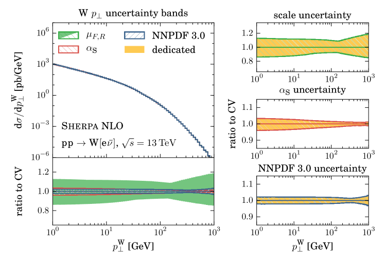
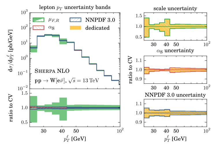
For the scale uncertainty band we employ a 7-point scale variation for $\mu_{R}$ and $\mu_{F}$: Both scales are varied independently by factors of $\nicefrac{{1}}{{2}}$ and 2, omitting the variations with ratios of 4 between the two scales. The uncertainty is then taken as the envelope of all variations. The $\alpha_{\text{s}}$ uncertainty band is generated by varying the numerical value of the starting point of the running coupling, $\alpha_{\text{s}}(m_{\mathup{{{Z}}}}^{2})$, to the following five values: $0.115$, $0.117$, $0.118$, $0.119$ and $0.121$. Note that this variation of $\alpha_{\text{s}}$ should also enter the PDF fit, and hence the PDFs are varied consistently. This is expected to extenuate the effect of the $\alpha_{\text{s}}$ variation in most cases, as the PDF of the varied $\alpha_{\text{s}}$ is still fitted to describe the same data as the PDF of the nominal $\alpha_{\text{s}}$. This consistent $\alpha_{\text{s}}$+PDF variation is also part of the PDF4LHC recommendations for LHC Run II [49]. The envelope of these $\alpha_{\text{s}}$+PDF variations is taken as the respective uncertainty. The pure PDF uncertainty estimate is generated using the average and the standard deviation over the $100$ PDF replicas provided by the NNPDF3.0 set (at a fixed value of $\alpha_{\text{s}}=0.118$). This corresponds to the $68\text{\,}\mathrm{\char 37\relax}$ confidence level. This set-up is repeated for later reference in Table 1, along with a CT14 PDF variant, which is used in later studies.

	nominal	variations	error band
PDF sets	CT14	56 Hessian error sets with a $90\text{\,}\mathrm{\char 37\relax}$ CL	Hessian
	NNPDF3.0	100 statistical replicas with a $68\text{\,}\mathrm{\char 37\relax}$ CL	statistical
$\alpha_{\text{s}}(m_{Z}^{2})$ value	0.118	0.115, 0.117, 0.119, 0.121	envelope
$\mu_{R}$/$\mu_{F}$ factors	$\left(\vphantom{\frac{1}{2}}1,1\right)$	$\left(\frac{1}{2},\frac{1}{2}\right)$, $\left(1,\frac{1}{2}\right)$, $\left(\frac{1}{2},1\right)$, $\left(\vphantom{\frac{1}{2}}2,1\right)$, $\left(\vphantom{\frac{1}{2}}1,2\right)$, $\left(\vphantom{\frac{1}{2}}2,2\right)$	envelope

Table 1: Variations, which are used for studies in this publication, with two variants depending on the PDF choice. Note that each $\alpha_{\text{s}}(m_{Z}^{2})$ value is used with its associated PDF set variant in the context of hadronic collisions.

Comparing the uncertainties for the $\mathup{{{W}}}$ $p_{\perp}$, we observe that the scale uncertainties are the largest, with relative deviations of $\mathcal{O}\left($10\text{\,}\mathrm{\char 37\relax}$\right)$. The relative deviations related to the PDF and the strong coupling do not exceed $\sim$3\text{\,}\mathrm{\char 37\relax}$$. The scale uncertainty exhibits a minimum for $$100\text{\,}\mathrm{GeV}$<p_{\perp}^{\mathup{{{W}}}}<$200\text{\,}\mathrm{GeV}$$. The reason is that the variations of $\mu_{F}$ alone cross the central value prediction in this range, such that only the $\mu_{R}$ variation contributes to the overall scale uncertainty here.

Note that $p_{\perp}^{\mathup{{{W}}}}=0$ at $\mathcal{O}\left(\alpha_{\text{s}}^{0}\right)$, and therefore only real-emission events contribute to the distribution. Hence, the observable is only described to leading-order. We introduce it here as a reference for our later validations including the parton-shower, which use this observable. For the current validation, we complement the discussion of the $\mathup{{{W}}}$ transverse momentum with the one of the lepton it decays to, as the region below $m_{\mathup{{{W}}}}/2$ is already filled at $\mathcal{O}\left(\alpha_{\text{s}}^{0}\right)$, and therefore we have in part a true next-to-leading description for this observable. In fact, the scale uncertainties are much larger in that region, especially towards the $m_{\mathup{{{W}}}}/2$ threshold, and at the lepton $p_{\perp}$ cut at $25\text{\,}\mathrm{GeV}$. This gives a more realistic picture of the perturbative uncertainties than in the leading-order region above the threshold.

The small panels on the right of Fig. 1 compare the uncertainty bands calculated using the reweighting approach to uncertainty bands where dedicated calculations have been done for each variation. We observe that all bands overlap perfectly for both observables. This is because the reweighting as presented above is exact and for all runs the same phase-space points could be used: The reweighted and the dedicated predictions for each variation are therefore equal, and so are the uncertainty bands.

3 Reweighting parton-shower calculations

If parton-showering is added to a LO calculation, the value of the observable is not evaluated at $\Phi_{B}$ any longer, but at $\mathrm{PS}(\Phi_{B})$, which denotes the phase-space point after showering. Applying this modification to eq. (2.1) yields

$$\langle O\rangle^{\text{{LoPs}}}=\int\text{d}\Phi_{B}\;\mathrm{B}(\Phi_{B})\;\mathrm{PS}(O,\Phi_{B})=\lim\limits_{N\to\infty}\,\frac{1}{N_{\text{trial}}}\;\sum\limits_{i=1}^{N}\mathrm{B}(\Phi_{B,i})\;\mathrm{PS}(O,\Phi_{B,i})\,.$$ (3.1)

Therefore the reweighting for $\mathrm{B}$ does not need to be altered, but the parton-shower emissions depend on the PDF, the strong coupling, their respective scale prefactors $k_{\alpha_{\text{s}}}$ and $k_{\scalebox{0.6}{$f$}}$ (detailed below) and the starting scale $\mu_{Q}$, i.e.

$$\mathrm{PS}(O,\Phi_{B})\equiv\mathrm{PS}(O,\Phi_{B};\mu_{Q}^{2})\equiv\mathrm{PS}(O,\Phi_{B};k_{\alpha_{\text{s}}},k_{\scalebox{0.6}{$f$}};\alpha_{\text{s}},f;\mu_{Q}^{2})\;.$$ (3.2)

In order to reweight the parton-shower emissions, we first need to identify its exact dependence structure. Schematically, it acts on the phase-space element in the following way

$$\mathrm{PS}(O,\Phi_{n};t^{\prime})=\;\Delta_{n}(t_{\text{IR}},t^{\prime})\,O(\Phi_{n})\vphantom{\int_{t}^{t}}+\int_{t_{\text{IR}}}^{t^{\prime}}\text{d}\Phi_{1}\;\mathrm{K}_{n}(\Phi_{1})\,\Delta_{n}(t,t^{\prime})\,\mathrm{PS}(O,\Phi_{n+1};t)\,,$$ (3.3)

where the Sudakov form factor of the $n$-parton state, $\Delta_{n}$, and its splitting kernel $\mathrm{K}_{n}$ have been introduced. While the first term describes the no-emission probability between the starting scale $t^{\prime}$ and the infrared cut-off $t_{\text{IR}}$ and therefore does not change the phase-space element, the second term describes the emission of a parton at scale $t$ in the configuration $\text{d}\Phi_{1}=\text{d}t\,\text{d}z\,\text{d}\phi\;J(t,z)$ (the integration boundaries are to be understood in this decomposition), leading to a configuration $\text{d}\Phi_{n+1}=\text{d}\Phi_{n}\cdot\text{d}\Phi_{1}$. The Jacobian $J$ is not relevant to the discussion here and is subsequently absorbed in the splitting kernel $\mathrm{K}_{n}$. As the emissions are ordered in $t$, the Sudakov form factor in the second term ensures that the current emission is the hardest after starting the evolution at $t^{\prime}$. Additional emissions may occur at smaller $t$ and are not resolved at this stage – they are described by the parton shower acting on the newly produced state $\Phi_{n+1}$ with the new starting scale $t$. In eq. (3.3) the dependences on $\alpha_{\text{s}}$, the PDFs, and their respective scale prefactors $k_{\alpha_{\text{s}}}$ and $k_{\scalebox{0.6}{$f$}}$ have been omitted for brevity. They directly carry over to the splitting kernel and the Sudakov form factor, according to

$$\begin{split}\Delta_{n}(t_{2},t_{1};k_{\alpha_{\text{s}}},k_{\scalebox{0.6}{$f$}};\alpha_{\text{s}},f)\,=\;\exp\left(-\int_{t_{2}}^{t_{1}}\text{d}\Phi_{1}\;\mathrm{K}_{n}(\Phi_{1};k_{\alpha_{\text{s}}},k_{\scalebox{0.6}{$f$}};\alpha_{\text{s}},f)\right)\,.\end{split}$$ (3.4)

When considering parton-shower emissions off NLO QCD matrix elements special emphasis has to be given to the first emission as described in Sec. 3.3 below.

3.1 Parton-shower dependence structure

$\displaystyle\int$Type	$\displaystyle z$	$\displaystyle y$	$\displaystyle x$	$\displaystyle(ij,k)\to(i,j,k)$	$\displaystyle c,c^{\prime}$
FF$\displaystyle\int\limits_{A}^{B}$	$\displaystyle\tilde{z}_{i}$	$\displaystyle y_{ij,k}$	$\displaystyle 1$	$(ij,k)\to(i,j,k)$	$\displaystyle a,a$
FI$\displaystyle\int\limits_{A}^{B}$	$\displaystyle\tilde{z}_{i}$	$\displaystyle\frac{1-x_{ij,a}}{x_{ij,a}}$	$\displaystyle x_{ij,a}$	$(ij,a)\to(i,j,a)$	$\displaystyle a,a$
IF$\displaystyle\int\limits_{A}^{B}$	$\displaystyle x_{jk,a}$	$\displaystyle\frac{u_{j}}{x_{jk,a}}$	$\displaystyle x_{jk,a}$	$(aj,k)\to(a,j,k)$	$\displaystyle aj,a$
II$\displaystyle\int\limits_{A}^{B}$	$\displaystyle x_{j,ab}$	$\displaystyle\frac{\tilde{v}_{j}}{x_{j,ab}}$	$\displaystyle x_{j,ab}$	$(aj,b)\to(a,j,b)$	$\displaystyle aj,a$

Table 2: Definition of the evolution and splitting variables for each dipole type. The fifth column lists the splitting process as seen from the Born process, $c$ and $c^{\prime}$ refer to the flavour of the initial state before and after the splitting process, respectively. The variables $y_{ij,k}$, $\tilde{z}_{i}$, $x_{ij,a}$, $x_{jk,a}$, $x_{j,ab}$, $u_{j}$ and $v_{j}$ are defined in [36, 37, 23].

The default parton shower of Sherpa, dubbed CSShower [23], is based on Catani–Seymour dipole factorisation [36, 37]. Each branching of an emitter parton into two daughters is witnessed by a spectator parton, which takes the recoil, and ensures that on-shell states are transferred into on-shell states and energy-momentum conservation is respected simultaneously. The emitter and spectator partons reside either in the initial-state (I) or final-state (F), such that four dipole types need to be distinguished: II, IF, FI and FF. In this notation, the first letter refers to emitter, and the second to the spectator parton. The no-branching probabilities are given by the four corresponding Sudakov form factors

$$\begin{split}\Delta_{n}(t_{2},t_{1};k_{\alpha_{\text{s}}},k_{\scalebox{0.6}{$f$}};\alpha_{\text{s}},f)\,=\;\prod\limits_{\text{type}\,\in\,\{\text{FF},\text{FI},\text{IF},\text{II}\}}\Delta_{n}^{\text{type}}(t_{2},t_{1};k_{\alpha_{\text{s}}},k_{\scalebox{0.6}{$f$}};\alpha_{\text{s}},f)\,.\end{split}$$ (3.5)

They share the common form

$$\begin{split}&\Delta_{n}^{\text{type}}(t_{2},t_{1};k_{\alpha_{\text{s}}},k_{\scalebox{0.6}{$f$}};\alpha_{\text{s}},f)\\ &\;=\exp\left(-\sum_{ij}\sum_{k}\int_{t_{2}}^{t_{1}}\text{d}t\int_{z_{-}}^{z_{+}}\text{d}z\;\alpha_{\text{s}}(k_{\alpha_{\text{s}}}t)\,\mathrm{K}^{\prime}_{ij,k}(t,z)\,\frac{f_{c^{\prime}}(\tfrac{\eta_{c}}{x},k_{\scalebox{0.6}{$f$}}t)}{f_{c}(\eta_{c},k_{\scalebox{0.6}{$f$}}t)}\right)\,,\end{split}$$ (3.6)

wherein the kinematics of the splitting are given by the default choice for $t=Q^{2}\,y\,z(1-z)$ in the massless case while the $\mathrm{K}^{\prime}_{ij,k}(t,z)$ denote the coupling and PDF stripped splitting kernels incorporating the remaining pieces of the $\mathrm{K}_{ij,k}$ and the Jacobian $J$ of the phase-space parametrisation. The precise definitions of the variables for each dipole type are given in Table 2. It directly follows that for FF-type dipole splittings the ratio of PDFs is simply unity. Eq. (3.6) further details the dependence on the $\alpha_{\text{s}}$ and PDF scale factors $k_{\alpha_{\text{s}}}$ and $k_{\scalebox{0.6}{$f$}}$. These multiplicative factors as well as their variations are assumed to be of order one, such that they do not induce spurious large logarithms. The generalisation to the massive case is straightforward and only involves generalised definitions of $t$, $x$, $y$ and $z$, cf. [23].

3.2 Reweighting trial emissions

To numerically integrate Sudakov form factors typically the Sudakov Veto Algorithm is used [50, 51, 52, 53, 54, 55]. Therein the integrands $\mathrm{K}$ found in the Sudakov form factors are replaced with integrable overestimates $\hat{\mathrm{K}}$. This is balanced by only accepting a proposed emission with probability $P_{\mathrm{acc}}=\mathrm{K}/\hat{\mathrm{K}}$. A multiplicative factor in $\mathrm{K}$ is therefore equivalent to a multiplicative factor in $P_{\mathrm{acc}}$ [52]. This observation is for example used to apply matrix-element corrections [54], where the splitting kernels are replaced with a real-emission-like kernel $\mathrm{R}/\mathrm{B}$. This is done a-posteriori, i.e. the event weight is multiplied by $(\mathrm{R}/\mathrm{B})/\mathrm{K}$, the emission itself is unchanged. The same method is also used in the Vincia parton shower to calculate uncertainty variations for different scales, finite terms of the antenna functions, ordering parameters and sub-leading colour corrections [28]. Here we employ this technique to account for variations of the strong-coupling parameter and the PDFs in the shower evolution of LO and NLO QCD matrix elements.

As has been laid out in the previous section, the emission kernels $\mathrm{K}$ depend linearly on $\alpha_{\text{s}}$ and on a ratio of parton densities $f_{c^{\prime}}(\eta_{c}/x,k_{\scalebox{0.6}{$f$}}t)/f_{c}(\eta_{c},k_{\scalebox{0.6}{$f$}}t)$. A change of PDFs $f\rightarrow\tilde{f}$, the strong coupling $\alpha_{\text{s}}\rightarrow\tilde{\alpha}_{\text{s}}$ and the scale prefactors entering both, i.e. $k_{\alpha_{\text{s}}}\to\tilde{k}_{\alpha_{\text{s}}}$ and $k_{\scalebox{0.6}{$f$}}\to\tilde{k}_{\scalebox{0.6}{$f$}}$, is equivalent to modifying the emission probability accordingly:

$$P_{\mathrm{acc}}\rightarrow q_{\mathrm{acc}}\,P_{\mathrm{acc}}\,,\qquad q_{\mathrm{acc}}\equiv\frac{\tilde{\alpha}_{\text{s}}(\tilde{k}_{\alpha_{\text{s}}}t)}{\alpha_{\text{s}}(k_{\alpha_{\text{s}}}t)}\;\frac{\tilde{f}_{c^{\prime}}(\tfrac{\eta_{c}}{x},\tilde{k}_{\scalebox{0.6}{$f$}}t)}{f_{c^{\prime}}(\tfrac{\eta_{c}}{x},k_{\scalebox{0.6}{$f$}}t)}\;\frac{f_{c}(\eta_{c},k_{\scalebox{0.6}{$f$}}t)}{\tilde{f}_{c}(\eta_{c},\tilde{k}_{\scalebox{0.6}{$f$}}t)}\,,$$ (3.7)

where the scale dependence and the definition of $\eta_{c}$ and $x$ can be read off the Sudakov form factors given in eq. (3.6) and Table 2. In case of FF dipoles eq. (3.7) simplifies significantly as the ratios of PDF factors reduces to unity. It further follows, that the event weight for each accepted emission needs to be multiplied by the corresponding factor $q_{\mathrm{acc}}$ in order to incorporate the new choice of $\alpha_{\text{s}}$, PDFs and the scales they are evaluated at. Accordingly, the probability to reject an emission is changed to

$$P_{\mathrm{rej}}=1-P_{\mathrm{acc}}\rightarrow 1-q_{\mathrm{acc}}P_{\mathrm{acc}}=\left[1+\left(1-q_{\mathrm{acc}}\right)\frac{P_{\mathrm{acc}}}{1-P_{\mathrm{acc}}}\right]\,P_{\mathrm{rej}}\equiv q_{\mathrm{rej}}\,P_{\mathrm{rej}}\,.$$ (3.8)

Consequently, for each rejected emission the event weight receives a corrective weight of $q_{\mathrm{rej}}$. Proofs that this treatment indeed results in the correct Sudakov form factors can be found in [52, 27, 26].

3.3 Next-to-leading-order matching

To match NLO QCD parton-level calculations with subsequent parton-shower evolution Sherpa employs a variant of the original Mc@Nlo algorithm presented in [12], referred to as S-Mc@Nlo [54]. Schematically, such a S-Mc@Nlo calculation has the following structure:

$$\begin{split}\langle O\rangle^{\text{{NloPs}}}\,=\;&\int\text{d}\Phi_{B}\;\left[\,\mathrm{B}(\Phi_{B})+\mathrm{VI}(\Phi_{B})+\int\text{d}x_{a/b}^{\prime}\,\mathrm{KP}(\Phi_{B},x_{a/b}^{\prime})\right.\\ &{}\qquad\qquad\left.+\sum_{j}\int\text{d}\Phi_{1}^{j}\,\left(\mathrm{D}_{A,j}-\mathrm{D}_{S,j}\right)(\Phi_{B}\cdot\Phi_{1}^{j})\right.\bigg{]}\,\mathrm{PS}_{\text{{NloPs}}}(O,\Phi_{B})\\ &{}+\int\text{d}\Phi_{R}\;\left[\vphantom{\sum_{j}}\,\mathrm{R}(\Phi_{R})-\sum_{j}\mathrm{D}_{A,j}(\Phi_{B,j}\cdot\Phi_{1}^{j})\right]\,\mathrm{PS}(O,\Phi_{R})\\ \,=\;&\int\text{d}\Phi_{B}\;\overline{\mathrm{B}}(\Phi_{B})\;\mathrm{PS}_{\text{{NloPs}}}(O,\Phi_{B})+\int\text{d}\Phi_{R}\;\mathrm{H}_{A}(\Phi_{R})\;\mathrm{PS}(O,\Phi_{R})\;.\end{split}$$ (3.9)

Here the real-emission contribution $\mathrm{R}$ of the NLO calculation has effectively been split into an infrared-singular (soft) and an infrared-regular (hard) part, the resummation kernel $\mathrm{D}_{A}$ and the finite hard remainder $\mathrm{H}_{A}$, respectively, such that $\mathrm{R}=\mathrm{D}_{A}+\mathrm{H}_{A}$  [57, 54]. The $\overline{\mathrm{B}}$-function has the following explicit parameter dependences

$$\begin{split}\overline{\mathrm{B}}(\Phi_{B})\,\equiv&\;\overline{\mathrm{B}}(\Phi_{B};\alpha_{\text{s}},f;\mu_{R},\mu_{F})\vphantom{\int}\\ \,=&\;\mathrm{B}(\Phi_{B};\alpha_{\text{s}},f;\mu_{R},\mu_{F})+\mathrm{VI}(\Phi_{B};\alpha_{\text{s}},f;\mu_{R},\mu_{F})\\ &{}+\int\text{d}x_{a/b}^{\prime}\,\mathrm{KP}(\Phi_{B},x_{a/b}^{\prime};\alpha_{\text{s}},f;\mu_{R},\mu_{F})\\ &{}+\sum_{j}\int\text{d}\Phi_{1}^{j}\;\left(\mathrm{D}_{A,j}-\mathrm{D}_{S,j}\right)(\Phi_{B}\cdot\Phi_{1}^{j};\alpha_{\text{s}},f;\mu_{R},\mu_{F})\;.\end{split}$$ (3.10)

From the perspective of parameter reweighting, the resummation kernel $\mathrm{D}_{A}$ behaves the same way as the subtraction term $\mathrm{D}_{S}$. In fact, in our reweighting implementation the $(\mathrm{D}_{A}-\mathrm{D}_{S})$ contribution is treated as a single term, as indicated. It is only to note that their PDFs are evaluated at the partonic momentum fraction $x_{a/b,j}$ and external flavours $a_{j}$ and $b_{j}$ of their $\Phi_{B}\cdot\Phi_{1}^{j}$ phase-space configuration rather than those of $\Phi_{B}$. The other parts of the $\overline{\mathrm{B}}$-function can then be reweighted as described in Sec. 2.2, leading to

$$\begin{split}\@ADDCLASS{ltx_eqn_lefteqn}$\displaystyle\overline{\mathrm{B}}(\Phi_{B};\tilde{\alpha}_{\text{s}},\tilde{f};\tilde{\mu}_{R},\tilde{\mu}_{F})\vphantom{\int}$\mbox{}\hfil\\ \,=\;&\tilde{\alpha}_{\text{s}}^{n}(\tilde{\mu}_{R}^{2})\;\tilde{f}_{a}(x_{a},\tilde{\mu}_{F}^{2})\;\tilde{f}_{b}(x_{b},\tilde{\mu}_{F}^{2})\;\\ &\times\;\left[\vphantom{\int}\mathrm{B}^{\prime}(\Phi_{B})+\tilde{\alpha}_{\text{s}}(\tilde{\mu}_{R}^{2})\left(\mathrm{VI}^{\prime}(\Phi_{B})+c_{R}^{\,\prime\,(0)}l_{R}+\tfrac{1}{2}\,c_{R}^{\,\prime\,(1)}l_{R}^{2}\right)\right.\\ &\left.\hskip 59.75078pt{}+\tilde{\alpha}_{\text{s}}(\tilde{\mu}_{R}^{2})\int\text{d}x_{a/b}^{\prime}\,\mathrm{KP}^{\prime}_{j}(\Phi_{j},x_{a/b}^{\prime};\tilde{f};\tilde{\mu}_{F,\text{core}})\right]\\ &{}+\sum_{j}\int\text{d}\Phi_{1}^{j}\;\tilde{f}_{a_{j}}(x_{a,j},\tilde{\mu}_{F}^{2})\;\tilde{f}_{b_{j}}(x_{b,j},\tilde{\mu}_{F}^{2})\;\tilde{\alpha}_{\text{s}}^{n+1}(\tilde{\mu}_{R}^{2})\;\left[\mathrm{D}_{A,j}^{\prime}-\mathrm{D}_{S,j}^{\prime}\right](\Phi_{B}\cdot\Phi_{1}^{j})\;.\end{split}$$ (3.11)

The $\mathrm{H}_{A}$-function then transforms as

$$\begin{split}\@ADDCLASS{ltx_eqn_lefteqn}$\displaystyle\mathrm{H}_{A}(\Phi_{R};\tilde{\alpha}_{\text{s}},\tilde{f};\tilde{\mu}_{R},\tilde{\mu}_{F})$\mbox{}\hfil\\ =\;&\mathrm{R}(\Phi_{R};\tilde{\alpha}_{\text{s}},\tilde{f};\tilde{\mu}_{R},\tilde{\mu}_{F})-\sum_{j}\mathrm{D}_{A,j}(\Phi_{B,j}\cdot\Phi_{1,j}^{j};\tilde{\alpha}_{\text{s}},\tilde{f};\tilde{\mu}_{R,j},\tilde{\mu}_{F,j})\\ =\;&\tilde{\alpha}_{\text{s}}^{n+1}(\tilde{\mu}_{R}^{2})\;\tilde{f}_{a}(x_{a},\tilde{\mu}_{F}^{2})\;\tilde{f}_{b}(x_{b},\tilde{\mu}_{F}^{2})\;\mathrm{R}^{\prime}(\Phi_{R})\\ &{}-\sum_{j}\tilde{\alpha}_{\text{s}}^{n+1}(\tilde{\mu}_{R,j}^{2})\;\tilde{f}_{a}(x_{a},\tilde{\mu}_{F,j}^{2})\;\tilde{f}_{b}(x_{b},\tilde{\mu}_{F,j}^{2})\;\mathrm{D}_{A,j}^{\prime}(\Phi_{B,j}\cdot\Phi_{1,j}^{j})\;,\end{split}$$ (3.12)

wherein each subtraction term $\mathrm{D}_{A,j}$ has its own scales $\mu_{R,j}$, $\mu_{F,j}$ defined on its underlying Born configuration $\Phi_{B,j}$. Writing eq. (3.9) as a Monte-Carlo sum over events with B-like and R-like structure, which are conventionally called $\mathds{S}$ and $\mathds{H}$ events in Mc@Nlo calculations, and with $N=N_{\mathds{S}}+N_{\mathds{H}}$, we obtain

$$\begin{split}\langle O\rangle^{\text{{NloPs}}}\,=&\;\lim\limits_{N\to\infty}\frac{1}{N_{\text{trial}}}\left\{\sum\limits_{i=1}^{N_{\mathds{S}}}\;\overline{\mathrm{B}}(\Phi_{B,i})\;\mathrm{PS}_{\text{{NloPs}}}(O,\Phi_{B,i})\right.\\ &\;\left.\hskip 65.44133pt{}+\sum\limits_{i=1}^{N_{\mathds{H}}}\;\mathrm{H}_{A}(\Phi_{R,i})\;\mathrm{PS}(O,\Phi_{R,i})\right\}\,.\end{split}$$ (3.13)

Thus, under $\mu_{R}\to\tilde{\mu}_{R}$, $\mu_{F}\to\tilde{\mu}_{F}$, $\alpha_{\text{s}}\to\tilde{\alpha}_{\text{s}}$ and $f\to\tilde{f}$ both $\overline{\mathrm{B}}$ of the $\mathds{S}$-events and $\mathrm{H}_{A}$ of the $\mathds{H}$-events transform as composite objects in terms of their constituents, as defined above. This leaves the S-Mc@Nlo parton shower, $\mathrm{PS}_{\text{{NloPs}}}$, defined through

$$\begin{split}\mathrm{PS}_{\text{{NloPs}}}(O,\Phi_{B})\equiv&\;\mathrm{PS}_{\text{{NloPs}}}(O,\Phi_{B};k_{\alpha_{\text{s}}},k_{\scalebox{0.6}{$f$}};\alpha_{\text{s}},f;\mu_{Q}^{2})\\ =&\;\overline{\Delta}_{n}(t_{\text{IR}},t^{\prime})\,O(\Phi_{n})\vphantom{\int_{t}^{t}}\\ &{}+\int_{t_{\text{IR}}}^{t^{\prime}}\text{d}\Phi_{1}\;\frac{\mathrm{D}_{A}(\Phi_{B}\cdot\Phi_{1})}{\mathrm{B}(\Phi_{B})}\;\overline{\Delta}_{n}(t,t^{\prime})\,\mathrm{PS}(O,\Phi_{n+1};t)\,.\end{split}$$ (3.14)

It differs from the usual $\mathrm{PS}$ of eq. (3.3) with respect to the splitting kernel for the first emission and the associated definition of the Sudakov form factor, cf. [54, 58]. However, for the purpose of reweighting, all trial emissions can be treated in the same way as in the standard parton shower as the parameter dependences are identical.

3.4 Validation

To validate the reweighting of scale and parameter dependences in CSShower and S-Mc@Nlo calculations within the Sherpa framework we perform closure tests between reweighting results and dedicated simulations.

Our implementation allows to constrain the maximum number of reweighted shower emissions per event. For a pure leading-order parton-shower run or $\mathds{H}$-like events in S-Mc@Nlo calculations this amounts to setting $n_{\text{PS}}\in\{0,1,2,\ldots,\infty\}$. When considering S-Mc@Nlo simulations in addition the parameter $n_{\textsc{NloPs}}\in\{0,1\}$ can be used to disable the reweighting of the $\cal{O}(\alpha_{\text{s}})$ emission for $\mathds{S}$-events.

Of course the reweighting result will only coincide with a dedicated calculation if all emissions are reweighted, i.e. $n_{\textsc{NloPs}}=1$ and $n_{\text{PS}}=\infty$. However, by subsequently enabling the reweighting of more and more emissions the relevance of their dependences for the determination of the full uncertainty can be studied. A finite value of $n_{\text{PS}}$ can also be useful in production, if the effect of reweighting higher-order emissions becomes negligible. The reduced amount of reweighting per event then allows for a faster event generation. An additional benefit would be that rare high-multiplicity shower histories do not spoil the statistical convergence of the reweighted result, even if their exact kinematics might be irrelevant for the studied observable.

The final-state only case: Thrust in $\mathup{{{e}}^{\scriptstyle{+}}}\mathup{{{e}}^{\scriptstyle{-}}}\mspace{1.0mu}\to\mspace{1.0mu}\mathit{{q}{}_{\mspace{-3.0mu}\scriptstyle{}}^{\mspace{-1.0mu}\scriptstyle{}}}\mathit{{\mkern 4.0mu\overline{\mkern-4.0mu{q}}}{}_{\mspace{-2.0mu}\scriptstyle{}}^{\mspace{0.0mu}\scriptstyle{}}}$ events

To validate LoPs reweighting, we consider two observables, which are complementary in their sensitivity to parton-shower emissions. At first, we consider the event-shape variable thrust $T$ [59] in hadronic events in $e^{+}e^{-}$-collisions at ${\sqrt{s}=$91.2\text{\,}\mathrm{G}\mathrm{e}\mathrm{V}$}$. In this case QCD emissions are restricted to the final-state. Accordingly, there appear no PDF factors in the shower reweighting, cf. eq. (3.7), and thus no factorisation scale dependence. Moreover, as we consider the leading-order matrix element for $e^{+}e^{-}\to q\bar{q}$ only, the renormalisation scale is also absent in the hard-process component. Therefore, we can concentrate on the pure $\alpha_{\text{s}}$ uncertainty in the parton shower here. Leaving the perturbative order of its running invariant it is defined by its value at the input scale $m_{Z}$.

Figure 2: Uncertainty band for the Thrust event shape in dijet production in $\mathup{{{e}}^{\scriptstyle{-}}}\mathup{{{e}}^{\scriptstyle{+}}}$ annihilation for a variation of $\alpha_{\text{s}}$. The left panel shows the nominal distribution and the ratio to the central value. The uncertainty band calculated using reweighting (including all emissions, i.e. $n_{\text{PS}}=\infty$) is compared to the one obtained from dedicated calculations. The comparison is repeated in the three panels on the right for different maximum number of reweighted emission $n_{\text{PS}}$.

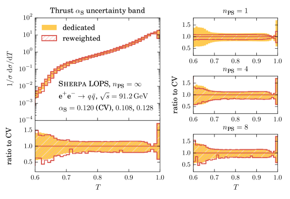
In Fig. 2, we compare $\alpha_{\text{s}}$ uncertainty bands generated by reweighting the nominal prediction with the one generated by dedicated predictions for each variation. As in Fig. 1, the uncertainty band is defined as the envelope over the distributions with different $\alpha_{\text{s}}(m_{Z}^{2})$ input values. The nominal value is taken as $\alpha_{\text{s}}(m_{Z}^{2})=0.120$, and its up/down variations are $0.128$ and $0.108$, respectively. Reweighting bands are presented for $n_{\text{PS}}=1,4,8,\infty$. The $n_{\text{PS}}=1$ band underestimates the uncertainty, especially for $T\leq 2/3$, where multiple hard emissions are required, and for $T\approx 1$, the region sensitive to multiple soft emissions. For $n_{\text{PS}}=4$, the uncertainty is underestimated only for bins with $T\leq 2/3$, and less so than for the $n_{\text{PS}}=1$ case. The difference between the two choices of $n_{\text{PS}}=8$ and $\infty$ is merely statistical and both reproduce the dedicated result very accurately.

Figure 3: The same as in Fig. 1, but for LO + parton-shower (PS) generation. The uncertainty bands are calculated by reweighting the ME and up to $n_{\text{PS}}$ shower emissions. In the upper four plots, $n_{\text{PS}}=3$. In the lower plots, $n_{\text{PS}}$ is varied for comparison. The scale uncertainties do not change with $n_{\text{PS}}$ and are therefore not repeated.

However, for low values of $T$, the statistical fluctuations of the reweighting results with higher $n_{\text{PS}}$ grow larger, corresponding to a widening of the distribution of reweighting factors. Low values of the thrust observable correspond to the emission of several hard partons, which is less probable in the parton-shower approximation, and more appropriately modelled in multijet-merged calculations, cf. Sec. 4. In this phase-space region it is difficult for the reweighting to compensate the multitude of accepted soft emissions off these hard legs, that turn unstable for $P_{\text{acc}}\to 1$, with rejected ones, cf. eq. (3.8). This issue can be addressed by introducing a prefactor for the over-estimator function $\hat{\mathrm{K}}$ in the reweighting runs, to ensure that $P_{\text{acc}}$ does not approach $1$, cf. [52, 27, 26]. This renders the Sudakov Veto Algorithm somewhat less efficient, but is shown to reduce statistical fluctuations in the reweighting.

The initial-state dominated case: $p_{\perp}^{\mathup{{{W}}}}$ in $\mathup{{{p}}}\mathup{{{p}}}\mspace{1.0mu}\to\mspace{1.0mu}\mathup{{{W}}}[\mathup{{{e}}}\mathit{{\nu}{}_{\mspace{-3.0mu}\scriptstyle{}}^{\mspace{-1.0mu}\scriptstyle{}}}]$ events

The second observable considered to validate our CSShower and S-Mc@Nlo reweighting implementation is the $\mathup{{{W}}}$-boson transverse-momentum distribution $p_{\perp}^{\mathup{{{W}}}}$ in $13\text{\,}\mathrm{TeV}$ proton-proton collisions, that has already been used in Sec. 2.3 in the NLO case. The definitions for constructing the uncertainty bands used there are kept the same, and are stated in Table 1. We now use the CT14nlo PDF set, which uses a Hessian error representation at a $90\text{\,}\mathrm{\char 37\relax}$ confidence level [60]. Therefore the PDF error band will be larger than before, as it now corresponds to nearly two standard deviations instead of only one.

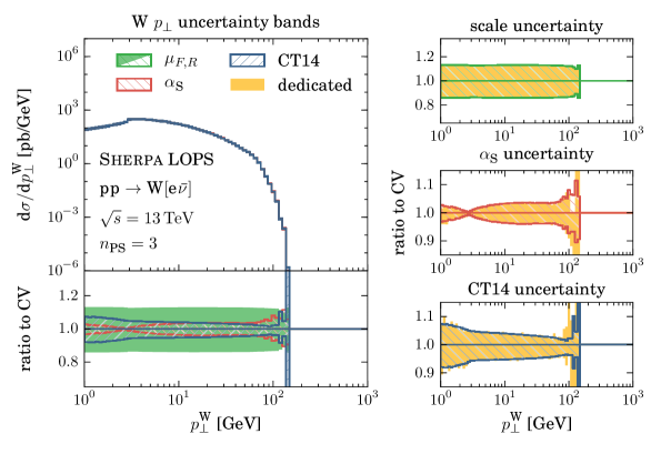
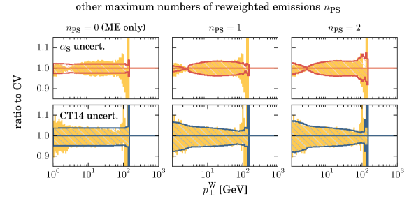
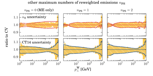
Considering a hadronic environment, initial-state emissions are present, which means that our reweighting factors now include PDF double ratios. In Fig. 3, we compare LoPs uncertainty bands for scale, $\alpha_{\text{s}}$ and PDF variations, including comparisons between reweighted and dedicated predictions for a varying maximum number of reweighted shower emissions $n_{\text{PS}}$. Before discussing the bands, we observe that the tail of the $p_{\perp}^{W}$ spectrum is not populated, in particular in comparison to Fig. 1. This is expected, as the LO configuration is restricted to $p_{\perp}^{W}=0$, such that all other bins are filled through recoils against parton-shower emissions only. However, the phase space of parton-shower emissions is restricted to the soft region, and therefore the $\mathup{{{W}}}$ boson can not build up a large recoil.

We now turn to the scale uncertainty band—which is entirely due to factorisation scale variations, because the LO matrix element is independent of $\alpha_{\text{s}}$ , and therefore the band underestimates the perturbative uncertainty. We also observe that the band is nearly flat. As we vary only the scales of the matrix-element calculation, the constant spread corresponds to the factorisation-scale uncertainty of the Born configuration at $p_{\perp}^{W}=0$, merely propagating to higher $p_{\perp}^{W}$ bins through the parton shower, which is unaware of the scale variations. In the matrix-element reweighting, we can guarantee the same phase-space points as in the dedicated run, such that we see perfect agreement between dedicated and reweighted predictions. We therefore omit comparisons for different $n_{\text{PS}}$ for the scale-uncertainty band.

Looking at the $\alpha_{\text{s}}$ uncertainty band, we can see that the envelope constricts at the position of the peak of the distributions. This reflects that the variation of $\alpha_{\text{s}}$ shifts the position of the peak, such that variations that are below the nominal distribution on the left side of the peak, are exceeding the nominal distribution on the right side, and vice versa. Comparing the reweighted prediction to the dedicated one, we find a flat band for $n_{\text{PS}}=0$, corresponding to restricting the reweighting to the fixed-order matrix element. As the LO calculation is independent of $\alpha_{\text{s}}$, this only reflects the change of the PDFs, which are fitted to $\alpha_{\text{s}}(m_{\mathup{{{Z}}}})$. The reproduction of the shape of the $\alpha_{\text{s}}$ uncertainty improves a lot when reweighting up to one emission ($n_{\text{PS}}=1$), and slightly more when adding another emission on top ($n_{\text{PS}}=2$).

For the PDF uncertainty, we see that the reweighting with $n_{\text{PS}}=0$ underestimates it by at least 1–$5\text{\,}\mathrm{\char 37\relax}$ for small transverse momenta, and overestimate it around the $\mathup{{{W}}}$ mass. As for the $\alpha_{\text{s}}$ uncertainty, this improves for $n_{\text{PS}}=1,2$.

The last depicted step, i.e. $n_{\text{PS}}=3$, on the other hand, does not contribute further to the reproduction of the $\alpha_{\text{s}}$ and PDF uncertainties. No significant differences with respect to the $n_{\text{PS}}=2$ case is observed. It can be concluded that it is sufficient to include up to two emissions to reproduce the uncertainty bands for this observable.

This is to be expected, as the gauge boson recoils against the shower emissions and is therefore mostly affected by the few hardest branchings. These mainly originate from the incoming hard virtual partons, so the generally softer final-state emissions barely contribute. Although we do not reproduce this here, we confirmed this by entirely disabling final-state emissions, which showed no effect on the results.

Figure 4: The same as in Fig. 3, but for NLO + parton-shower (PS) generation. The uncertainty bands are calculated by reweighting the ME and a maximum number of emissions from the Mc@Nlo ($n_{\textsc{NloPs}}$) and the ordinary PS ($n_{\text{PS}}$). $n_{\textsc{NloPs}}$ is constrained to 0 or 1, as the Mc@Nlo prescription only affects the first emission. In the upper four plots we consider $n_{\textsc{NloPs}}=1$ and $n_{\text{PS}}=2$, thus up to three emissions get reweighted. In the lower plots, we consider variations of $n_{\textsc{NloPs}}$ and $n_{\text{PS}}$.

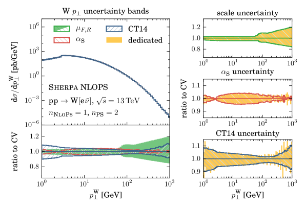
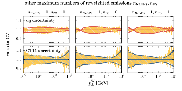
In Fig. 4 we present the validation of NloPs predictions for the $\mathup{{{W}}}$-boson transverse-momentum distribution. Overall, we get a similar picture as in the LoPs case. The main differences are the increased high-$p_{\perp}^{\mathup{{{W}}}}$ reach and the significantly smaller scale uncertainties in the low $p_{\perp}^{\mathup{{{W}}}}$ range, a consequence of including the complete set of $\cal{O}(\alpha_{\text{s}})$ corrections to the production process. For large $p_{\perp}^{\mathup{{{W}}}}$, the uncertainty increases again, because we fall back to a LO description again: Only the $2\to 3$ matrix element still contributes.

To assess the quality of the reweighting, we consider again different settings for the parameters $n_{\textsc{NloPs}}$ and $n_{\text{PS}}$. Assuming $n_{\textsc{NloPs}}=n_{\text{PS}}=0$, only the scale variations of the hard process are considered and the parton-shower contribution to the $\cal{O}(\alpha_{\text{s}})$ correction is not reweighted. Furthermore, we present results for $n_{\textsc{NloPs}}=1$ and $n_{\text{PS}}=0,1,2$. With these settings, the $\cal{O}(\alpha_{\text{s}})$ corrections get properly reweighted, but the number of subsequent shower emissions off the $\mathds{S}$- and $\mathds{H}$-like events treated correctly is varied. We observe a saturation for reproducing the dedicated calculations at $n_{\textsc{NloPs}}+n_{\text{PS}}\geq 2$, with no further improvement when $n_{\text{PS}}$ is increased from $1$ to $2$. This confirms the findings made when considering the LoPs setup in Fig. 3: The gauge-boson transverse-momentum distribution is dominated by the few hardest emissions.

4 Reweighting multijet-merged calculations

In this section we address the reweighting of multijet-merged event generation runs. These approaches allow to combine LO or NLO QCD matrix elements of different multiplicity dressed with parton showers into inclusive samples. Accordingly, the production of jets associating a given core process can be modelled through exact matrix elements rather than relying on the logarithmic approximation of the parton shower only. In particular, when considering hard jet kinematics or angular correlations such techniques prove to be indispensable to properly describe experimental observations, see for instance [61, 62, 63, 64].

To first approximation the reweighting as described in the previous sections can be used without change, only that the perturbative order $p$ is no longer a constant across the sample, but varies for each event, corresponding to the considered matrix-element parton multiplicity. However, there are also new algorithm-specific intricacies which complicate the dependence on the input parameters and need to be dealt with to allow for a consistent reweighting. The LO and NLO merging techniques employed within the Sherpa framework are presented in [21] and [65, 66], respectively. They rely on the reconstruction of parton-shower histories for multi-parton amplitudes that set the parton-shower initial conditions for their subsequent evolution. This is achieved by running a backward-clustering algorithm that identifies a corresponding core process and calculates hard-parton splitting scales that serve as predetermined shower branchings. In the Sherpa approach the actual parton shower then starts off the reconstructed core process and implements the predetermined hard splittings based on a truncated shower. Furthermore, it is the purpose of the truncated-shower evolution to implement possible Sudakov vetoes for shower emissions above the phase-space separation or merging scale $Q_{\text{cut}}$. It should be emphasised here, parton-shower reweighting is vital when using modified input parameters in order to cancel the $Q_{\text{cut}}$ dependence to the accuracy of the parton shower. In case only the hard-process matrix element parameters get reweighted, the dependence on $Q_{\text{cut}}$ is cancelled to leading-logarithmic accuracy only, however, residual subleading contributions from the running coupling or the PDF evolution remain [65].

For the reweighting of the truncated-shower Sudakov veto probability the methods described in Sec. 3 can be applied. In what follows we will detail the specifics of the reweighting procedure for LO and NLO multijet-merging runs with Sherpa supplemented by an extensive validation of the implementation.

4.1 Preliminaries

Figure 5: Possible parton-shower histories of a $qg\to Zgqq^{\prime}\bar{q}^{\prime}$ matrix element allowing only QCD splittings (left) and also including electroweak splittings (right).

Common to the LO and NLO merging techniques used in Sherpa, cf. [21, 22, 65, 66, 67], is the separation of the emission phase space into a soft and a hard region, defined through a suitable $m$-parton measure $Q_{m}$ and a separation criterion $Q_{\text{cut}}$. For each parton configuration $\Phi_{m}$ with $Q_{m}>Q_{\text{cut}}$ a shower history that represents the event as a core process with subsequent $1\to 2$ shower splittings is probabilistically build through backward clustering. The resulting sequence of cluster steps is characterised by tuples $\{a_{i},b_{i},x_{a,i},x_{b,i},t_{i}\}$, recording the (possibly changing) initial-state flavours and momentum fractions as well as the evolution variable of each splitting. We allow for both QCD and EW splitting functions [21, 68] to identify such splitting processes and veto recombinations that would lead to the reduction of configurations which are not present in the matrix elements. Figure 5 details possible cluster histories for a given $\mathup{{{p}}}\mathup{{{p}}}\mspace{1.0mu}\to\mspace{1.0mu}\mathup{{{Z}}}+4\,\text{jets}$ configuration, depending on its kinematics, allowing for QCD splittings only (left) or both QCD and EW splittings (right).

The sequence $\{t_{i}\}$ of reconstructed branching scales then may be either ordered or unordered, with an ordered history satisfying $t_{j}<t_{j-1}<\ldots<t_{1}<t_{0}=\mu_{F,\text{core}}^{2}$. The recombination probabilities in each clustering step are determined by the forward-splitting probabilities and are therefore dependent on the parton shower and its parameters and choices. This is reflected, step-by-step, in the addition of one factor of $\alpha_{\text{s}}$ (when appropriate) at the reconstructed splitting scale, a ratio of PDFs at the reconstructed initial flavours and their momentum fractions, and a Sudakov form factor describing the evolution of each step.

In the Sherpa implementations the $\alpha_{\text{s}}$ and PDF factors are added explicitly onto the respective matrix elements and can therefore be reweighted directly. The Sudakov form factor, on the other hand, is implemented through a vetoed truncated parton shower [21, 22]. The truncated shower itself, accounting for the possibility of soft parton-shower emissions between subsequent reconstructed hard emissions, i.e. with $t_{m}<t<t_{m-1}$ but $Q<Q_{\text{cut}}$, can be reweighted with the methods described in Sec. 3. If, however, an emission with $Q>Q_{\text{cut}}$ occurs the event is vetoed. Practically, this is accounted for through increasing $n_{\text{trial}}$ of the next accepted event by $n_{\text{trial}}$ of the vetoed event. Thus, $n_{\text{trial}}$ becomes dependent on the parton-shower parameters.

A special remark concerning unordered histories, i.e. histories whose sequence of $\{t_{i}\}$ has at least one pair $t_{k}\geq t_{k-1}$, is in order. Such histories can be encountered in various configurations, e.g. when the last clustering step produces a splitting scale larger than the nominal starting scale of the core process or the flavour structure only allows further clusterings at scales $t_{k-1}$ lower than the last identified one $t_{k}$. As such configurations cannot be generated by a strictly ordered parton shower, for each unordered step neither the accompanying PDF ratio nor Sudakov factor is therefore present in the calculation. More than one unordering in a cluster history of a given event is possible and in fact likely at high multiplicities. PDF ratios and Sudakov factors then of course only occur in the ordered subhistories in between the unorderings. For the sake of clarity and brevity we will omit this case from the discussion of the following subsections. Its implications to the algorithm, and therefore to the reweighting, are straightforward. If ordered histories are enforced, core configurations beyond the standard $2\to 2$ processes occur. Independent of the presence and number of unorderings, the renormalisation and factorisation scales $\mu_{R}$ and $\mu_{F}$ are always set in the way, as will be detailed below.

4.2 The leading-order case

We start the discussion with the simplest case, where all matrix elements used in the merging are given at leading order. A LO multijet-merged calculation, with Born matrix elements at $\mathcal{O}\left(\alpha_{\text{s}}^{n+j}\right)$, containing $j$ additional partons relative to the core process, has the following structure

$$\begin{split}\langle O\rangle^{\text{{MePs@Lo}}}\,=&\;\sum_{j=0}^{j_{\text{max}}}\int\text{d}\Phi_{j}\;\mathrm{B}^{\text{merge}}_{j}(\Phi_{j})\;\Theta(Q_{j}-Q_{\text{cut}})\;\mathrm{PS}^{\text{vt}}(O,\Phi_{j})\\ \,=&\;\lim\limits_{N\to\infty}\,\frac{1}{N_{\text{trial}}}\sum_{i=1}^{N}\sum_{j=0}^{j_{\text{max}}}\mathrm{B}^{\text{merge}}_{j}(\Phi_{j,i})\;\Theta(Q_{j}-Q_{\text{cut}})\;\mathrm{PS}^{\text{vt}}(O,\Phi_{j,i})\;.\end{split}$$ (4.1)

Note that $\Phi_{j}$ here denotes the entire final-state phase space of the process, including all particles of the core process. As before, $Q_{j}$ is a suitable infrared-safe distance measure of $\Phi_{j}$. The $\Theta$-function thus realises a minimum separation of $Q_{\text{cut}}$ and acts as an infrared regulator. $\mathrm{PS}^{\text{vt}}$ is the vetoed truncated parton shower derived from eq. (3.3). As the limit in the second line is well defined, it can be transposed with the summation over parton multiplicities. As the ingredient leading-order matrix elements need to incorporate the soft-collinear resummation properties of the parton shower, they have the following parameter dependences:

$$\begin{split}\mathrm{B}^{\text{merge}}_{j}(\Phi_{j})\,\equiv&\;\mathrm{B}^{\text{merge}}_{j}(\Phi_{j};\alpha_{\text{s}},f;\mu_{R,\text{core}},\mu_{F,\text{core}},k_{\alpha_{\text{s}}},k_{\scalebox{0.6}{$f$}};\{a_{i},b_{i},x_{a,i},x_{b,i},t_{i}\})\,.\end{split}$$ (4.2)

The cluster steps $\{a_{i},b_{i},x_{a,i},x_{b,i},t_{i}\}$ denote the identified cluster history of the configuration $\Phi_{j}$, as discussed above. Therein, the $a_{i},\,b_{i}$ are the possibly changing initial-state flavours, the $x_{a,i},\,x_{b,i}$ their momentum fractions, and the $t_{i}$ are the reconstructed values of the parton-shower evolution variable at each splitting. Together with the $\alpha_{\text{s}}$ and PDF scale prefactors $k_{\alpha_{\text{s}}}$, $k_{\scalebox{0.6}{$f$}}$ of the parton shower, the cluster steps relate $\mathrm{B}^{\text{merge}}_{j}$ to the scale and PDF stripped Born matrix element $\mathrm{B}^{\prime}_{j}$ encountered in Sec. 2.1,

$$\begin{split}\@ADDCLASS{ltx_eqn_lefteqn}$\displaystyle\mathrm{B}^{\text{merge}}_{j}(\Phi_{j};\alpha_{\text{s}},f;\mu_{R,\text{core}},\mu_{F,\text{core}},k_{\alpha_{\text{s}}},k_{\scalebox{0.6}{$f$}};\{a_{i},b_{i},x_{a,i},x_{b,i},t_{i}\})$\mbox{}\hfil\\ \,=\;&\prod\limits_{i=1}^{j}\frac{f_{a_{i}}(x_{a,i},k_{\scalebox{0.6}{$f$}}t_{i})}{f_{a_{i-1}}(x_{a,i-1},k_{\scalebox{0.6}{$f$}}t_{i})}\;f_{a_{0}}(x_{a,0},\mu_{F,\text{core}}^{2})\prod\limits_{i=1}^{j}\frac{f_{b_{i}}(x_{b,i},k_{\scalebox{0.6}{$f$}}t_{i})}{f_{b_{i-1}}(x_{b,i-1},k_{\scalebox{0.6}{$f$}}t_{i})}\;f_{b_{0}}(x_{b,0},\mu_{F,\text{core}}^{2})\\ &\times\;\alpha_{\text{s}}^{n+j}(\mu_{R}^{2})\;\mathrm{B}^{\prime}_{j}(\Phi_{j})\,.\end{split}$$ (4.3)

In this notation, the core scale is $t_{0}=\mu_{F,\text{core}}^{2}$, it is therefore not multiplied by the prefactors of the parton shower. The partonic momentum fractions of the core process are $x_{a,0},\,x_{b,0}$.

The scales of each single $\alpha_{\text{s}}$ within the cluster history vary, but an effective global renormalisation scale can be defined through

$$\begin{split}\alpha_{\text{s}}^{n+j}(\mu_{R}^{2})=\alpha_{\text{s}}^{n+e}(\mu_{R,\text{core}}^{2})\;\prod_{i=1}^{j}\alpha_{\text{s}}^{1-\epsilon_{i}}(k_{\alpha_{\text{s}}}t_{i})\,,\end{split}$$ (4.4)

where $\epsilon_{i}=0$ if the identified splitting process at branching $i$ is of QCD-type, and $1$ otherwise, $e=\sum_{i=1}^{j}\epsilon_{i}$. To consistently vary the $\mu_{R}$ scale, we consider variations of the splitting scales $t_{i}$ and the core scale $\mu_{R,\text{core}}$ on the right-hand side by a common factor, solving for the prefactor of the effective $\mu_{R}$ to be used in the matrix-element calculation. Thus, while up to NLO accuracy $\mu_{R}$ is varied by the same common factor, the full solution of this procedure results in slightly larger variations of the effective renormalisation scale.

Apart from the Sudakov form factors the soft-collinear structure of the $\mathrm{B}^{\text{merge}}_{j}$ is now identical to the emission of $j$ partons off a $\mathrm{B}_{0}$ configuration with the parton shower described in section 3. In case of final-state splittings the ratio of parton distribution functions is simply unity as neither the partonic $x_{a/b,i}$ and $x_{a/b,i-1}$ nor the initial-state flavours $a_{i},\,b_{i}$ and $a_{i-1},\,b_{i-1}$ differ. In principle, with every ratio of PDFs there is also a ratio of flux factors. However, all such factors cancel except for the outermost ones, corresponding to $\Phi_{j}$ and, hence, are regarded as part of $\mathrm{B}^{\prime}_{j}$.

Changing the scales $\mu_{R,\text{core}}\to\tilde{\mu}_{R,\text{core}}$, $\mu_{F,\text{core}}\to\tilde{\mu}_{F,\text{core}}$, $k_{\alpha_{\text{s}}}\to\tilde{k}_{\alpha_{\text{s}}}$, $k_{\scalebox{0.6}{$f$}}\to\tilde{k}_{\scalebox{0.6}{$f$}}$ as well as $\alpha_{\text{s}}\to\tilde{\alpha}_{\text{s}}$ and $f\to\tilde{f}$ results in

$$\begin{split}\@ADDCLASS{ltx_eqn_lefteqn}$\displaystyle\mathrm{B}^{\text{merge}}_{j}(\Phi_{j};\tilde{\alpha}_{\text{s}},\tilde{f};\tilde{\mu}_{R,\text{core}},\tilde{\mu}_{F,\text{core}},\tilde{k}_{\alpha_{\text{s}}},\tilde{k}_{\scalebox{0.6}{$f$}};\{a_{i},b_{i},x_{a,i},x_{b,i},t_{i}\})$\mbox{}\hfil\\ \,=\;&\prod\limits_{i=1}^{j}\frac{\tilde{f}_{a_{i}}(x_{a,i},\tilde{k}_{\scalebox{0.6}{$f$}}t_{i})}{\tilde{f}_{a_{i-1}}(x_{a,i-1},\tilde{k}_{\scalebox{0.6}{$f$}}t_{i})}\;\tilde{f}_{a_{0}}(x_{a,0},\tilde{\mu}_{F,\text{core}}^{2})\prod\limits_{i=1}^{j}\frac{\tilde{f}_{b_{i}}(x_{b,i},\tilde{k}_{\scalebox{0.6}{$f$}}t_{i})}{\tilde{f}_{b_{i-1}}(x_{b,i-1},\tilde{k}_{\scalebox{0.6}{$f$}}t_{i})}\;\tilde{f}_{b_{0}}(x_{b,0},\tilde{\mu}_{F,\text{core}}^{2})\\ &\times\;\tilde{\alpha}_{\text{s}}^{n+j}(\tilde{\mu}_{R}^{2})\;\mathrm{B}^{\prime}_{j}(\Phi_{j})\,.\end{split}$$ (4.5)

The scale $\tilde{\mu}_{R}^{2}$ is now calculated from eq. (4.4) using $\tilde{\mu}_{R,\text{core}}^{2}$ and $\tilde{k}_{\alpha_{\text{s}}}$ as input.

Eq. (4.5) describes what happens to the matrix-element part of a multijet-merged calculation. This leaves the vetoed truncated shower $\mathrm{PS}^{\text{vt}}$. While the truncated and standard shower part is described in section 3, the vetoed shower leads to vetoed events. As vetoed events correspond to events whose weights have been set to zero, their description is equivalent to increasing the number of trials, $n_{\text{trial}}$, by one. Thus, when varying the parameters of the parton shower, also the probabilities of vetoing events are changed. Consequently, $n_{\text{trial}}$ acquires a dependence on the parameters of the variation. Thus, now explicitly stating the dependence on the shower’s starting scale $\mu_{Q}^{2}$ and the merging scale $Q_{\text{cut}}$,

$$\begin{split}\@ADDCLASS{ltx_eqn_lefteqn}$\displaystyle n_{\text{trial}}(\mu_{Q}^{2};Q_{\text{cut}}^{2};\{a_{i},b_{i},x_{a,i},x_{b,i},t_{i}\})$\mbox{}\hfil\\ \,\equiv&\;n_{\text{trial}}(\mu_{Q}^{2};Q_{\text{cut}}^{2};\{a_{i},b_{i},x_{a,i},x_{b,i},t_{i}\};\alpha_{\text{s}},f;k_{\alpha_{\text{s}}},k_{\scalebox{0.6}{$f$}})\\ \,=&\;\frac{1-\Delta_{n+j}(t_{\text{IR}},\mu_{Q}^{2};Q_{\text{cut}}^{2};\tilde{\alpha}_{\text{s}},\tilde{f};\tilde{k}_{\alpha_{\text{s}}},\tilde{k}_{\scalebox{0.6}{$f$}};\{a_{i},b_{i},x_{a,i},x_{b,i},t_{i}\})}{1-\Delta_{n+j}(t_{\text{IR}},\mu_{Q}^{2};Q_{\text{cut}}^{2};\alpha_{\text{s}},f;k_{\alpha_{\text{s}}},k_{\scalebox{0.6}{$f$}};\{a_{i},b_{i},x_{a,i},x_{b,i},t_{i}\})}\,,\end{split}$$ (4.6)

where

$$\begin{split}\@ADDCLASS{ltx_eqn_lefteqn}$\displaystyle\Delta_{n+j}(t_{\text{IR}},\mu_{Q}^{2};Q_{\text{cut}}^{2};\alpha_{\text{s}},f;k_{\alpha_{\text{s}}},k_{\scalebox{0.6}{$f$}};\{a_{i},b_{i},x_{a,i},x_{b,i},t_{i}\})$\mbox{}\hfil\\ \,=&\;\prod\limits_{i=1}^{j}\exp\left\{-\int\limits_{t_{i}}^{t_{i-1}}\text{d}\Phi_{1}\;\mathrm{K}_{n+i}(\Phi_{1};k_{\alpha_{\text{s}}},k_{\scalebox{0.6}{$f$}};\alpha_{\text{s}},f)\;\Theta(Q_{n+i}>Q_{\text{cut}})\right\}\;.\end{split}$$ (4.7)

Thus, $n_{\text{trial}}$ corresponds to the survival probability between the unfolding of preexisting splittings when evolving from the $n$-parton core configuration to the $(n+j)$-parton configuration. Hence, when changing the parameters of the simulation the truncated showers probability to emit a parton with $Q>Q_{\text{cut}}$ must be re-evaluated following the substitutions $k_{\alpha_{\text{s}}}\to\tilde{k}_{\alpha_{\text{s}}}$, $k_{\scalebox{0.6}{$f$}}\to\tilde{k}_{\scalebox{0.6}{$f$}}$, $\alpha_{\text{s}}\to\tilde{\alpha}_{\text{s}}$ and $f\to\tilde{f}$ using the methods of Sec. 3. Note, all emissions produced by the truncated shower prior to the one that triggers the veto need to be reweighted as they impact the initial conditions for that emission.

4.3 The next-to-leading-order case

The merging of multijet matrix elements at next-to-leading order accuracy proceeds schematically similar as in the leading order case. The input quantity is now the NloPs matched $(n+j)$-parton configuration, thus

$$\begin{split}\langle O\rangle^{\text{{MePs@Nlo}}}\,=&\;\sum_{j=0}^{j_{\text{max}}}\left[\int\text{d}\Phi_{j}\;\overline{\mathrm{B}}^{\text{merge}}_{j}(\Phi_{j})\;\Theta(Q_{j}-Q_{\text{cut}})\;\mathrm{PS}_{\text{{NloPs}}}^{\text{v}}(O,\Phi_{j})\right.\\ &\left.\hskip 28.45274pt{}+\int\text{d}\Phi_{j+1}\;\mathrm{H}_{A,j}^{\text{merge}}(\Phi_{j+1},Q_{\text{cut}})\;\mathrm{PS}^{\text{vt}}(O,\Phi_{j+1})\right]\\ \,=&\;\lim\limits_{N\to\infty}\,\frac{1}{N_{\text{trial}}}\left\{\sum\limits_{i=1}^{N_{\mathds{S}}}\sum\limits_{j=0}^{j_{\text{max}}}\;\overline{\mathrm{B}}^{\text{merge}}_{j}(\Phi_{j,i})\;\Theta(Q_{j}-Q_{\text{cut}})\;\mathrm{PS}_{\text{{NloPs}}}^{\text{v}}(O,\Phi_{j,i})\right.\\ &\left.\hskip 65.44133pt{}+\sum\limits_{i=1}^{N_{\mathds{H}}}\sum\limits_{j=0}^{j_{\text{max}}}\;\mathrm{H}_{A,j}^{\text{merge}}(\Phi_{j+1,i},Q_{\text{cut}})\;\mathrm{PS}^{\text{vt}}(O,\Phi_{j+1,i})\right\}\,,\end{split}$$ (4.8)

keeping the notation of eqs. (3.9) and (4.1). For the $\mathds{S}$-events the same $\Theta$-function of eq. (4.1) is used as an infrared regulator and the S-Mc@Nlo parton shower of eq. (3.14) is replaced by its vetoed version, it only matches the softest emission in $t$ and, thus, does not generate truncated emissions. These are added dressing it with additional emissions through the standard parton shower. As all ingredients of $\overline{\mathrm{B}}^{\text{merge}}_{j}$ are evaluated at the same phase-space point $\Phi_{j}$ they share a common cluster history $\{a_{i},b_{i},x_{a,i},x_{b,i},$ $t_{i}\}$. Hence, again suppressing any further $Q_{\text{cut}}$-dependence which is not varied,

$$\begin{split}\overline{\mathrm{B}}^{\text{merge}}_{j}(\Phi_{j})\equiv&\;\overline{\mathrm{B}}^{\text{merge}}_{j}(\Phi_{j};\alpha_{\text{s}},f;\mu_{R,\text{core}},\mu_{F,\text{core}},k_{\alpha_{\text{s}}},k_{\scalebox{0.6}{$f$}};\{a_{i},b_{i},x_{a,i},x_{b,i},t_{i}\})\end{split}$$ (4.9)

transforms under the replacements $k_{\alpha_{\text{s}}}\to\tilde{k}_{\alpha_{\text{s}}}$, $k_{\scalebox{0.6}{$f$}}\to\tilde{k}_{\scalebox{0.6}{$f$}}$, $\alpha_{\text{s}}\to\tilde{\alpha}_{\text{s}}$ and $f\to\tilde{f}$ in the following way:

$$\begin{split}\@ADDCLASS{ltx_eqn_lefteqn}$\displaystyle\overline{\mathrm{B}}^{\text{merge}}_{j}(\Phi_{j};\tilde{\alpha}_{\text{s}},\tilde{f};\tilde{\mu}_{R,\text{core}},\tilde{\mu}_{F,\text{core}},\tilde{k}_{\alpha_{\text{s}}},\tilde{k}_{\scalebox{0.6}{$f$}};\{a_{i},b_{i},x_{a,i},x_{b,i},t_{i}\})$\mbox{}\hfil\\ =\;&\prod\limits_{i=1}^{j}\frac{\tilde{f}_{a_{i}}(x_{a,i},\tilde{k}_{\scalebox{0.6}{$f$}}t_{i})}{\tilde{f}_{a_{i-1}}(x_{a,i-1},\tilde{k}_{\scalebox{0.6}{$f$}}t_{i})}\;\tilde{f}_{a_{0}}(x_{a,0},\tilde{\mu}_{F,\text{core}}^{2})\\ &\quad\times\prod\limits_{i=1}^{j}\frac{\tilde{f}_{b_{i}}(x_{b,i},\tilde{k}_{\scalebox{0.6}{$f$}}t_{i})}{\tilde{f}_{b_{i-1}}(x_{b,i-1},\tilde{k}_{\scalebox{0.6}{$f$}}t_{i})}\;f_{b_{0}}(x_{b,0},\tilde{\mu}_{F,\text{core}}^{2})\\ &\quad\times\;\tilde{\alpha}_{\text{s}}^{n+j}(\tilde{\mu}_{R}^{2})\;\left[\mathrm{B}^{\prime}_{j}(\Phi_{j})+\tilde{\alpha}_{\text{s}}(\tilde{\mu}_{R}^{2})\left(\mathrm{VI}^{\prime}_{j}(\Phi_{j})+c_{R,j}^{\,\prime\,(0)}l_{R}+\tfrac{1}{2}\,c_{R,j}^{\,\prime\,(1)}l_{R}^{2}\right)\vphantom{\int}\right.\\ &\left.\hskip 121.49326pt{}+\tilde{\alpha}_{\text{s}}(\tilde{\mu}_{R}^{2})\int\text{d}x_{a/b}^{\prime}\,\mathrm{KP}^{\prime}_{j}(\Phi_{j},x_{a/b}^{\prime};\tilde{f};\tilde{\mu}_{F,\text{core}})\right.\\ &\left.\hskip 121.49326pt{}+\tilde{\alpha}_{\text{s}}(\tilde{\mu}_{R}^{2})\sum_{k}\int\text{d}\Phi_{1}^{k}\left(\mathrm{D}_{A,k}^{\prime}-\mathrm{D}_{S,k}^{\prime}\right)(\Phi_{j}\cdot\Phi_{1}^{k})\right.\bigg{]}\\ &{}-\sum_{i=1}^{j}\frac{\tilde{\alpha}_{\text{s}}(\tilde{\mu}_{R}^{2})}{2\pi}\,\log\frac{t_{i-1}}{t_{i}}\left(\sum\limits_{c=q,g}\int\frac{\text{d}x_{a,i}^{\prime}}{x_{a,i}^{\prime}}\;P_{ac}(x_{a,i}^{\prime})\,\tilde{f}_{c}(\tfrac{x_{a,i}}{x_{a,i}^{\prime}},\tilde{k}_{\scalebox{0.6}{$f$}}t_{i})\right.\\ &\left.\hskip 119.50157pt{}+\sum\limits_{d=q,g}\int\frac{\text{d}x_{b,i}^{\prime}}{x_{b,i}^{\prime}}\;P_{bd}(x_{b,i}^{\prime})\,\tilde{f}_{d}(\tfrac{x_{b,i}}{x_{b,i}^{\prime}},\tilde{k}_{\scalebox{0.6}{$f$}}t_{i})\right)\tilde{\alpha}_{\text{s}}^{n+j}(\tilde{\mu}_{R}^{2})\,\mathrm{B}^{\prime}_{j}(\Phi_{j})\,.\end{split}$$ (4.10)

In addition to the transformation properties of the $\overline{\mathrm{B}}$-function of eq. (3.10), supplemented with the PDF ratios already encountered in the leading-order case, additional terms appear. They subtract the $\mathcal{O}\left(\alpha_{\text{s}}\right)$ expansion of these ratios, in order to retain the NLO accuracy of the merged calculation. Again, please note $t_{0}=\mu_{F,\text{core}}^{2}$.

The same does not hold, however, for the $\mathds{H}$-events. Their constituent real-emission matrix elements are defined on $\Phi_{j+1}$ , while each subtraction term $\mathrm{D}_{A,k}$ has its own projection on a phase-space point $\Phi_{j}^{k}$. Thus,

$$\begin{split}\@ADDCLASS{ltx_eqn_lefteqn}$\displaystyle\mathrm{H}_{A,j}^{\text{merge}}(\Phi_{j+1},Q_{\text{cut}})$\mbox{}\hfil\\ \,\equiv&\;\mathrm{R}^{\text{merge}}_{j}(\Phi_{j+1};\alpha_{\text{s}},f;\mu_{R,\text{core}},\mu_{F,\text{core}},k_{\alpha_{\text{s}}},k_{\scalebox{0.6}{$f$}};\{a_{i},b_{i},x_{a,i},x_{b,i},t_{i}\})\;\Theta(Q_{j}-Q_{\text{cut}})\\ &{}-\sum_{k}\mathrm{D}_{A,k,j}^{\text{merge}}(\Phi_{j}^{k}\cdot\Phi_{1}^{k};\alpha_{\text{s}},f;\mu_{R,\text{core},k},\mu_{F,\text{core},k},k_{\alpha_{\text{s}},k},k_{\scalebox{0.6}{$f$},k};\\[-8.53581pt] &\hskip 108.12047pt\{a_{i,k},b_{i,k},x_{a,i,k},x_{b,i,k},t_{i,k}\})\\ &\hskip 34.1433pt\times\;\Theta(Q_{j}^{k}-Q_{\text{cut}})\,,\end{split}$$ (4.11)

wherein both $\mathrm{R}^{\text{merge}}_{j}$ and the $\mathrm{D}_{A,k,j}^{\text{merge}}$ separately transform as the leading-order counterpart $\mathrm{B}^{\text{merge}}_{j}$. While the measure $Q$ on $\Phi_{j+1}$ of $\mathrm{R}^{\text{merge}}_{j}$ is defined to act on the underlying $\Phi_{j}$ after the first cluster step where the real emission configuration has been reduced to a Born configuration, it is defined directly on each $\Phi_{j}^{k}$ in each $\mathrm{D}_{A,k}$. Infrared safety is guaranteed through the infrared safety of their phase-space maps, the clustering algorithm and the measure $Q$.

Finally, we consider merging additional multiplicities up to ${j_{\text{max}}}$ described through leading-order matrix elements on top of a next-to-leading order merged calculation with up to ${j_{\text{max}}^{\text{{nlo}}}}$ jets, where ${j_{\text{max}}}>{j_{\text{max}}^{\text{{nlo}}}}$. The method of choice was outlined in [69, 22, 65, 66, 70] and is historically referred to as MeNloPs. Its methodology is defined as

$$\begin{split}\@ADDCLASS{ltx_eqn_lefteqn}$\displaystyle\langle O\rangle^{\text{{MePs@Nlo}{}+{MeNloPs}}}$\mbox{}\hfil\\ \,=&\;\sum_{j=0}^{j_{\text{max}}^{\text{{nlo}}}}\left[\int\text{d}\Phi_{j}\;\overline{\mathrm{B}}^{\text{merge}}_{j}(\Phi_{j})\;\mathrm{PS}_{\text{{NloPs}}}^{\text{v}}(O,\Phi_{j})\right.\\ &\left.\hskip 28.45274pt{}+\int\text{d}\Phi_{j+1}\;\mathrm{H}_{A,j}^{\text{merge}}(\Phi_{j+1})\;\mathrm{PS}^{\text{vt}}(O,\Phi_{j+1})\right]\\ &{}+\sum_{j={j_{\text{max}}^{\text{{nlo}}}}+1}^{j_{\text{max}}}\int\text{d}\Phi_{j}\;k_{j_{\text{max}}^{\text{{nlo}}}}(\Phi_{{j_{\text{max}}^{\text{{nlo}}}}+1}(\Phi_{j}))\;\mathrm{B}^{\text{merge}}_{j}(\Phi_{j})\;\mathrm{PS}^{\text{vt}}(O,\Phi_{j})\\ \,=&\;\lim\limits_{N\to\infty}\,\frac{1}{N_{\text{trial}}}\left\{\sum\limits_{i=1}^{N_{\mathds{S}}}\sum\limits_{j=0}^{j_{\text{max}}^{\text{{nlo}}}}\;\overline{\mathrm{B}}^{\text{merge}}_{j}(\Phi_{j,i})\;\mathrm{PS}_{\text{{NloPs}}}^{\text{v}}(O,\Phi_{j,i})\right.\\ &\left.\hskip 65.44133pt{}+\sum\limits_{i=1}^{N_{\mathds{H}}}\sum\limits_{j=0}^{j_{\text{max}}^{\text{{nlo}}}}\;\mathrm{H}_{A,j}^{\text{merge}}(\Phi_{j+1,i})\;\mathrm{PS}^{\text{vt}}(O,\Phi_{j+1,i})\right.\\ &\left.\hskip 65.44133pt{}+\sum_{i=1}^{N_{\text{LO}}}\sum_{j={j_{\text{max}}^{\text{{nlo}}}}+1}^{{j_{\text{max}}}}\;k_{j_{\text{max}}^{\text{{nlo}}}}(\Phi_{{j_{\text{max}}^{\text{{nlo}}}}+1}(\Phi_{j}))\;\mathrm{B}^{\text{merge}}_{j}(\Phi_{j,i})\;\mathrm{PS}^{\text{vt}}(O,\Phi_{j,i})\right\}\,,\end{split}$$ (4.12)

with $N=N_{\mathds{S}}+N_{\mathds{H}}+N_{\text{LO}}$. A differential $K$-factor $k_{j_{\text{max}}^{\text{{nlo}}}}$ is a applied to the higher-multiplicity leading-order matrix elements in order to facilitate a smooth transition across $Q_{\text{cut}}$. It has the form

$$\begin{split}k_{m}(\Phi_{m+1})\,=&\;\frac{\overline{\mathrm{B}}_{m}(\Phi_{m})}{\mathrm{B}_{m}(\Phi_{m})}\left(1-\frac{\mathrm{H}_{A,m}(\Phi_{m+1})}{\mathrm{R}_{m}(\Phi_{m+1})}\right)+\frac{\mathrm{H}_{A,m}(\Phi_{m+1})}{\mathrm{R}_{m}(\Phi_{m+1})}\;,\end{split}$$ (4.13)

and therefore moulds the $\mathrm{B}_{{j_{\text{max}}^{\text{{nlo}}}}+1}$ into the same form as the $\mathrm{H}_{A,{j_{\text{max}}^{\text{{nlo}}}}}$ it is replacing. The projection $\Phi_{{j_{\text{max}}^{\text{{nlo}}}}+1}(\Phi_{j})$ for $j>{j_{\text{max}}^{\text{{nlo}}}}+1$ is defined through its cluster history, as is $\Phi_{m}(\Phi_{m+1})$ inside $k_{m}$ itself. When now changing the parameters of the calculation, $\alpha_{\text{s}}\to\tilde{\alpha}_{\text{s}}$, $f\to\tilde{f}$, $\mu_{R}\to\tilde{\mu}_{R}$ and $\mu_{F}\to\tilde{\mu}_{F}$, $k_{j_{\text{max}}^{\text{{nlo}}}}$ transforms as a composite object in terms of its constituents, cf. Sec. 2 and 3. The scales are set directly by the $\mathrm{B}^{\text{merge}}_{j}$ process. Of course, in the interest of decreased computational costs one may decide to choose $k_{m}\equiv 1$ throughout at the cost of larger merging systematics. Similarly, if an electroweak cluster history leads to a changed signature in $\Phi_{m+1}$, $k_{m}\equiv 1$ is chosen.

4.4 Validation

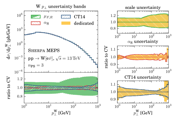
The reweighting for multijet-merged calculations as discussed in the previous sections has been implemented within Sherpa with the CSShower for leading-order matrix elements (MePs@Lo), next-to-leading order matrix elements (MePs@Nlo) and next-to-leading-order matrix elements with additional leading-order ones on top (MeNloPs). For the validation, we again perform closure tests between reweighted and dedicated predictions for the transverse momentum of the $\mathup{{{W}}}$ boson in Figs. 6, 7 and 8. As before, the uncertainty bands are the ones defined in Table 1, with the CT14 PDF set. For all merged calculations, we employ a merging cut of $Q_{\text{cut}}=$20\text{\,}\mathrm{G}\mathrm{e}\mathrm{V}$$.

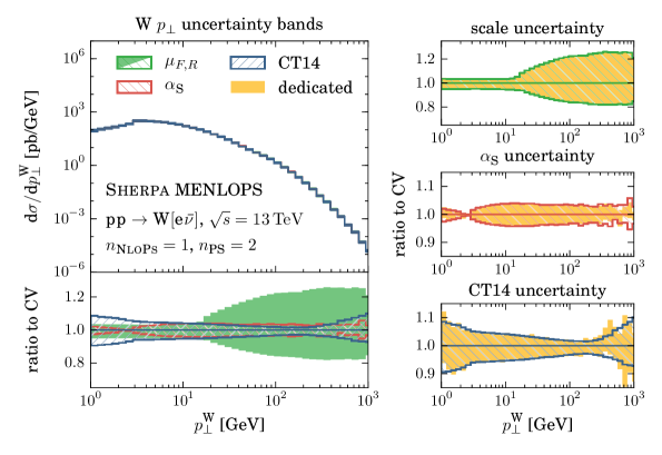
For the MePs@Lo validation in Fig. 6, we combine LO matrix elements for 0-, 1- and 2-jet multiplicities, obtained from Comix [39]. We can observe that we populate a much larger phase space than for a mere LoPs calculation in terms of $p_{\perp}^{\mathup{{{W}}}}$. Below the merging cut (i.e. $p_{\perp}^{\mathup{{{W}}}}\lesssim$20\text{\,}\mathrm{G}\mathrm{e}\mathrm{V}$$), the scale uncertainty band is equal to the one of the LoPs calculation. For higher $p_{\perp}^{\mathup{{{W}}}}$, the scale uncertainty increases corresponding to the larger uncertainty of the higher-multiplicity matrix elements, that contribute renormalisation scale uncertainties.

Figure 6: The same as in Figs. 3 and  4, but for a multijet-merged generation with LO matrix elements for 0-, 1- and 2-jet multiplicities. The uncertainty bands are calculated by reweighting the ME and a maximum number of emissions $n_{\text{PS}}$ of PS emissions. In the upper four plots, $n_{\text{PS}}=3$, thus up to three emissions are reweighted. In the lower plots, $n_{\text{PS}}$ is varied for comparison. Again, we find a saturation when reproducing dedicated calculations for $n_{\text{PS}}\geq 2$, with no further improvement when $n_{\text{PS}}$ is increased from 2 to 3.

Figure 7: The same as in Figs. 3, 4 and 6, but for a multijet-merged generation with one NLO matrix element for the 0-jet multiplicity, and LO matrix elements for the 1- and 2-jet multiplicities. The uncertainty bands are calculated by reweighting the ME and a maximum number of emissions from the Mc@Nlo ($n_{\textsc{NloPs}}$) and the ordinary PS ($n_{\text{PS}}$). In the upper four plots, $n_{\textsc{NloPs}}=1$ and $n_{\text{PS}}=2$, thus up to three emissions are reweighted. In the lower plots, both $n$ are varied for comparison. Again, we find a saturation when reproducing dedicated calculations for $n_{\textsc{NloPs}}+n_{\text{PS}}\geq 2$, with no further improvement when $n_{\text{PS}}$ is increased from 1 to 2.

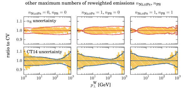
In Fig. 7, we consider the MeNloPs case. We combine an NLO matrix element for the 0-jet multiplicities with LO matrix elements for the 1- and 2-jet multiplicities. The scale uncertainty for low $p_{\perp}^{\mathup{{{W}}}}$ values now features the reduced scale uncertainty, that we already have seen in the NloPs validation.

Figure 8: The same as in Figs. 3, 4, 6 and 7, but for a multijet merged generation with NLO matrix elements for the 0- and 1-jet multiplicities. The uncertainty bands are calculated by reweighting the ME and a maximum number of emissions from the Mc@Nlo ($n_{\textsc{NloPs}}$) and the ordinary PS ($n_{\text{PS}}$). In the upper four plots, $n_{\textsc{NloPs}}=1$ and $=n_{\text{PS}}=2$, thus up to three emissions are reweighted. In the lower plots, both $n$ are varied for comparison. Again, we find a saturation when reproducing dedicated calculations for $n_{\textsc{NloPs}}+n_{\text{PS}}\geq 2$, with no further improvement when $n_{\text{PS}}$ is increased from 1 to 2.

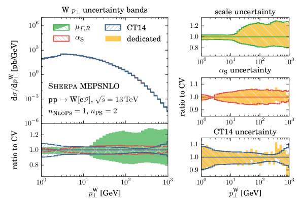
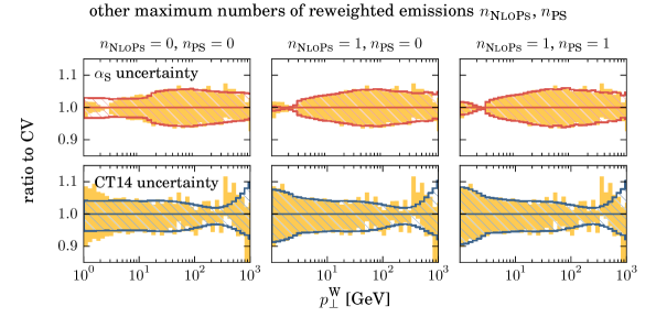
The same is true in the MePs@Nlo case depicted in Fig. 8. A direct comparison of the scale uncertainties to the MeNloPs case is not straightforward though, as we combine NLO matrix elements for the 0- and the 1-jet multiplicity, where the virtual amplitudes are obtained from BlackHat [42]. Hence, the 2-jet multiplicity is described at leading order through the 1-jet $\mathds{H}$-events. As such, the set-up is not a simple upgrade from our MeNloPs calculation.

In all multijet-merging validations, we find a similar behaviour with respect to the imprint of including emissions in the reweighting. For $n_{\textsc{NloPs}}+n_{\mathrm{PS}}=2$, the dedicated calculations are well reproduced, and no further improvement is found for $n_{\textsc{NloPs}}+n_{\mathrm{PS}}=3$. It is noteworthy, that for the MeNloPs case we find a worse reproduction for $n_{\textsc{NloPs}}=1$ and $n_{\mathrm{PS}}=0$ compared to the NloPs and the MePs@Nlo cases. This originates in the fact that in the latter two cases, we enable the reweighting of emissions off $\mathds{S}$-events at all involved multiplicities, whereas in the MeNloPs case only the first of the three multiplicities is affected, because the other two are at LO and therefore do not have $\mathds{S}$-events. Thus, the overall importance of the $\mathds{S}$ emission reweighting gets restricted to the region below $Q_{\text{cut}}$ of the 1-jet configuration in the MeNloPs case.

5 Consistent variations

In general, the renormalisation and factorisation scales, $\alpha_{s}$ and the PDFs should be varied consistently throughout any of the presented calculations. While at fixed order the situation is clear, the matched and merged approaches allow for some degree of freedom regarding partial variations while still retaining their respective accuracies.

In the simplest case, LOPS, $\mu_{R}$ and $\mu_{F}$ of the short distance cross section and the parton shower may be varied independently as these variations can be expressed as higher-order terms in a perturbative expansion in the coupling parameter $\alpha_{s}$. This is not the case for $\alpha_{s}$ itself and the PDFs as they are fixed through measured input values and parametrisations. Changes in these input values cannot be expressed as simple higher-order terms. Thus they need to be chosen consistently throughout.

Similarly, in NLOPS calculations, the renormalisation and factorisation scales may be varied in the matrix element ($\overline{\mathrm{B}}$ and $\mathrm{H}_{A}$) or the parton shower ($\mathrm{PS}_{\text{{NloPs}}}$ and $\mathrm{PS}$) separately without losing neither the fixed-order nor the resummation accuracy. As the pseudo-subtraction through the $\mathrm{D}_{A}$ in any case employs different scales in $\mathrm{PS}_{\text{{NloPs}}}$ and the $\overline{\mathrm{B}}$ and $\mathrm{H}_{A}$ functions, it always leaves remainders of $\mathcal{O}(\alpha_{s}^{2})$. Hence, further scale variations in either one, the short-distance cross sections or the $\mathrm{PS}_{\text{{NloPs}}}$, do not worsen the nominal accuracy of the method. Retaining the logarithmic accuracy of the parton shower on the other hand requires identical renormalisation and factorisation scales throughout all resummation-relevant components, i.e. $\mathrm{PS}_{\text{{NloPs}}}$ and $\mathrm{PS}$. Again, variations in $\alpha_{s}$ or the PDFs need to be consistent throughout the calculation.

The multijet-merged calculations impose further constraints since they treat multijet matrix elements and parton-shower emissions on the same footing. The notation of the scales already reflects this for $\mu_{R}$ and $\mu_{F}$. In their definitions only the core scales remain as free parameters and may be varied independently. Again, the $\alpha_{s}$ and PDF parametrisations need to be the same throughout.

6 Conclusions

In this publication we have presented the implementation and validation of reweighting techniques allowing for the fast and efficient evaluation of perturbative systematic uncertainties in the Sherpa event-generator framework. We have lifted the available techniques for the determination of PDF, $\alpha_{s}$ and scale uncertainties in leading- and next-to-leading order QCD calculations to include the respective variations in parton-shower simulations. In turn we provide the means to perform consistent uncertainty evaluations for multijet-merged simulations based on leading- or next-to-leading-order accurate matrix elements of varying multiplicity matched with parton showers. The foundation for our reweighting method is the knowledge of the very dependence structure of the perturbative calculations on the parameters to be varied. For the fixed-order components this amounts to the corresponding decomposition of the Catani–Seymour dipole subtraction terms. This needed to be supplemented by the reweighting of the parametric dependences of the parton shower treated through the Sudakov Veto Algorithm.

With our extensive validation we have been able to prove on the one-hand-side the correctness of the implementation and have, furthermore, been able to illustrate the importance of parton-shower reweighting for reliable uncertainty estimates. With comparably little additional computational costs this allows for the on-the-fly determination of PDF, $\alpha_{S}$ and scale uncertainties based on one single generator run, that, otherwise, would require explicit re-computations. The overall reduction in CPU time is by a factor of about 3 to 20, depending on the event-generation mode used, see App. A. The variational event weights provided are easily accessible through the HepMC event record and are furthermore consistently handed over to the Rivet analysis software by the corresponding Sherpa interface.

The methods presented in this publication are ideally suited for event-wise uncertainty estimates and can readily be used in arbitrary theoretical and experimental analyses. An extension to next-to-next-to-leading-order QCD calculations possibly dressed with parton showers, as presented in [16, 17, 71], is straightforward and planned for the near future.

The decomposition of the fixed-order part of QCD calculations employed here is also a necessary ingredient to produce cross-section grids as provided by the APPLgrid [72] and FastNLO [73, 74] tools. These store the perturbative coefficients for a certain observable calculation discretised in $Q^{2}$ and $x$. Using interpolation methods, this allows for the a posteriori inclusion of PDFs, $\alpha_{\text{s}}$ and variations of the renormalisation and factorisation scales. In turn, such techniques are well suited for (combined) fits of PDFs and $\alpha_{\text{s}}$ that require a multitude of re-computations of the theoretical predictions. Over the last years, tools have been developed that automate the projection of arbitrary next-to-leading-order QCD calculations onto such grids, namely the aMCfast [75] and the MCgrid [76, 77, 78] packages. The first one produces APPLgrids with MadGraph5_aMC@NLO [79], the latter APPLgrids or FastNLO grids from Sherpa events projected on the observables through Rivet. The APFELgrid tool [80] provides an improved convolution method for use with APPLgrid files that furthermore speeds-up the re-evaluations.

However, none of these approaches includes generic parton-shower effects, i.e. the parametric dependence of the shower component on the PDFs and $\alpha_{\text{s}}$ is ignored. With the methods presented in this publication we are confident that we can surmount this limitation and in the future provide interpolation grids that properly reflect shower-resummation effects and allow for the inclusion of the affected phase-space regions in PDF determinations.

Appendix A CPU time measurements

The benefit of reweighted calculations is given by the saving of CPU time. In order to evaluate the gain, we shall compare the event generation time of reweighted calculations with the sum of generation times for all corresponding dedicated computations. Here we consider both parton-level calculations, as well as runs including multiple interactions and hadronisation, the typical default in physics analyses applications. For the latter it can be expected that the gain in CPU time by using the reweighting approach is most considerable, as the CPU intense non-perturbative event generation phases do not need to be re-evaluated. In what follows we compare actual event-generation times, neglecting the set-up times of the individual runs.

In Fig. 9, we consider event generations using LoPs, NloPs, MePs@Lo and MePs@Nlo calculations for $\mathup{{{p}}}\mathup{{{p}}}\mspace{1.0mu}\to\mspace{1.0mu}\mathup{{{W}}}[\mathup{{{e}}^{\scriptstyle{-}}}\mathit{{\mkern 4.0mu\overline{\mkern-4.0mu{\nu}}}{}_{\mspace{-2.0mu}\scriptstyle{}}^{\mspace{0.0mu}\scriptstyle{}}}]$ at $13\text{\,}\mathrm{TeV}$. The ratio of CPU time between the reweighting and the dedicated generations is shown for different maximum numbers of reweighted shower emissions $n_{\text{PS}}+n_{\textsc{NloPs}}$. Whether non-perturbative effects are included or not, the time needed for the reweighting calculation is below $10\text{\,}\mathrm{\char 37\relax}$ of the time needed for dedicated calculations if only the matrix element is reweighted ($n_{\text{PS}}=n_{\textsc{NloPs}}=0$). The ratio then increases for larger numbers of reweighted emissions, as their reweighting needs additional time, asymptotically approaching the value when all parton-shower emissions are reweighted. For parton-level-only calculations, this ratio is around $0.35$ for LoPs events, and around $0.3$ for NloPs events. This reduction can be explained due to relatively smaller computational cost of the parton shower as a whole when the rest of the calculation is more complex. Also note that $n_{\text{PS}}$ for LoPs is only equivalent to $n_{\text{PS}}+n_{\textsc{NloPs}}$ for $\mathcal{S}$ events. $\mathcal{H}$ events do not feature the S-Mc@Nlo-emission, and hence for them $n_{\textsc{NloPs}}$ does not contribute to their reweighting.

Figure 9: The ratio of CPU time needed for a reweighting event generation $t_{\text{rew}}$ over the time needed for generating predictions for all variations with dedicated runs $t_{\text{ded}}$. The reweighting includes up to $n_{\text{PS}}+n_{\textsc{NloPs}}$ parton-shower emissions. The sampled variations are listed in Tab. 1. Parton-level-only results are compared to results for calculations including multiple interactions and hadronisation effects (“+ non-perturbative”), and to calculations where in addition to adding non-perturbative effects the events have also been unweighted (“+ unweighting”). The ratios for reweighting all emissions are indicated with a horizontal line.

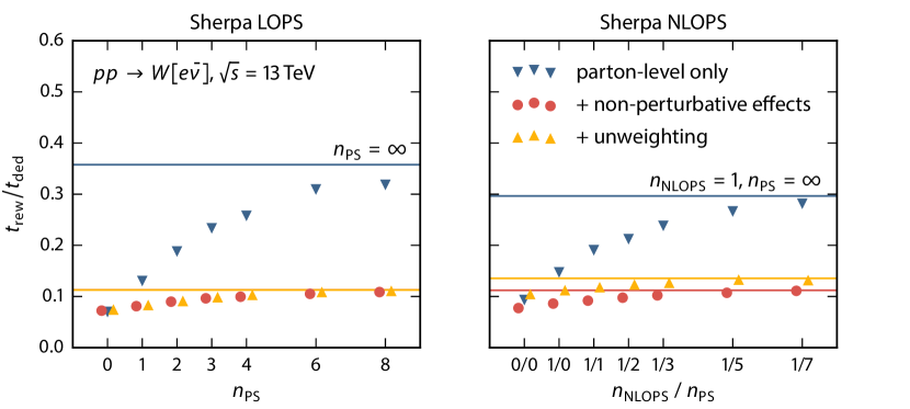
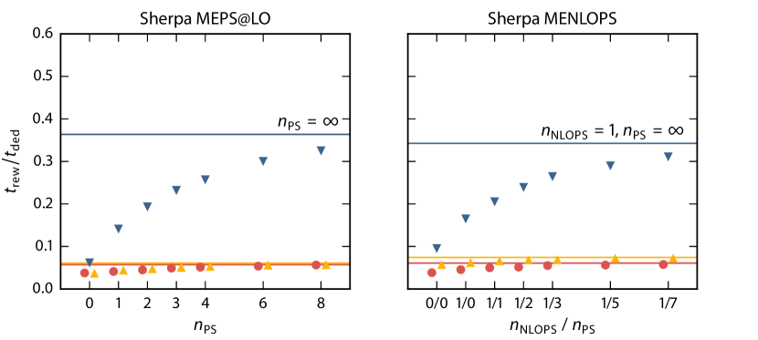
For the same reason, when non-perturbative effects are included, that ratio improves to about $0.1$: The parton shower (and its reweighting) component plays a relatively smaller rôle in terms of CPU cycles, when multiple interactions and hadronisation are enabled.

If on top of the non-perturbative effects the events are also unweighted, the ratio does not change in the LoPs case, but in the NloPs case (by about $20\text{\,}\mathrm{\char 37\relax}$). A reason might be, that only for NloPs a sizeable number of events gets rejected. For these, the jet evolution and non-perturbative phases are not performed at all, whereas the matrix-element calculation (and its reweighting) is always done, for accepted and rejected events alike. The same is true for the S-Mc@Nlo emission from $\mathds{S}$ events. As a consequence, the relative cost of the reweighting grows slightly. A future improvement of the implementation would postpone these futile reweightings in unweighted calculations to a time point after the possible rejection. This of course requires that the dependence of the rejection probability is negligible. For the observables studied so far this was found to be true, at least to $\mathcal{O}\left(10^{-4}\right)$.

Note that the effective gains will be lower than the results presented in this section, when we take into account the reduced statistical accuracy which comes with the parton-shower reweighting. This requires more events to be generated in a reweighting calculation to reach the same statistical accuracy as in a dedicated calculation.

Appendix B Configuring and accessing event-weight variations

Sherpa provides a list of pre-calculated alternative event weights, which are automatically output to the HepMC event record [24] or directly to an interfaced Rivet analysis [25]. For versions of Sherpa later than v.2.2.0, the variations to calculate can be specified with the following line in the (run) section of the Sherpa run card:

  VARIATIONS muR2fac1,muF2fac1,PDF1 muR2fac2,muF2fac2,PDF2 ...;

Each variation is characterised by up to three arguments

muR2fac

a prefactor multiplying the nominal (squared) renormalisation scale

muF2fac

a prefactor multiplying the nominal (squared) factorisation scale

PDF

a parton density and its accompanying $\alpha_{\text{s}}$ parametrisation.

This syntax works for all employed scale setters of Sherpa and both Sherpa’s internal PDFs and PDFs interfaced through Lhapdf5/6 [81, 82]. If trailing arguments are omitted from a variation, their default values are used, which is 1.0 for scale factors and the PDF set used by Sherpa for the nominal calculation.

In HepMC event records (v. 2.06 or later), the alternate weights can be accessed as named weights within the HepMC::WeightContainer of each event. The keys are given in one of the following formats:

    MUR<muR2fac>_MUF<muF2fac>_PDF<ID>
    MUR<muR2fac>_MUF<muF2fac>_PDF<ID>_PSMUR<muR2fac>_PSMUF<muF2fac>

The parts in angle brackets are replaced with the respective scale factors and Lhapdf IDs. The second form is used, if a factor is applied to the renormalisation/factorisation scale of parton-shower splittings. This includes splittings within cluster histories determined by the multijet merging procedure, as discussed in section 4. If the scale reweighting with parton-shower splittings has been enabled (we discuss below how to do so), the scale factors for MUR, MUF and PSMUR, PSMUF are always equal, respectively, in the current implementation.

If the internal Rivet interface of Sherpa is used to analyse events during the generation, one histogram file per variation is written to disk, along with the nominal one. The file names follow a pattern resembling the HepMC weight-container keys as specified above.

Scale variations

The scale argument can also be specified by enclosing it in square brackets: [mu2fac]. This syntactic sugar implies both the given factor, its inverse and the default value. For example, 1.0,[4.0] is equivalent to 1.0,4.0 1.0,0.25 1.0,1.0 and therefore triggers up and down variations of the factorisation scale, along with the central value. If both scale factors are enclosed in brackets, they are expanded individually, keeping the other at its default value of 1.0: Hence, [4.0],[4.0] is equivalent to the 5-point scale variation 4.0,1.0 0.25,1.0 1.0,4.0 1.0,0.25 1.0,1.0. To include simultaneous variations in the same direction, both factors can be surrounded by a single pair of brackets. Thus, [4.0,4.0] is equivalent to the 7-point scale variation 4.0,1.0 0.25,1.0 1.0,4.0 1.0,0.25 4.0,4.0 0.25,0.25 1.0,1.0.

PDF and $\alpha_{\text{s}}$ variations

PDF and $\alpha_{\text{s}}$ variations both work by specifying a PDF set through the PDF argument of a variation. This is because Sherpa per default uses the value for $\alpha_{\text{s}}(m^{2}_{Z})$ given by the PDF set in use. Therefore an $\alpha_{\text{s}}$ variation can be achieved by using PDF fits for different values of $\alpha_{\text{s}}(m^{2}_{Z})$.

To specify a specific member of a PDF set, its number is given as an additional argument separated by a slash. Thus, 1.0,1.0,CT14nlo/38 asks for the 38th member of the CT14nlo PDF set, without modifying the renormalisation and factorisation scales. If the slash and the number are not given, the central PDF member is used, i.e. CT14nlo is equivalent to CT14nlo/0.

Sherpa can also be asked to do variations for all members of a PDF set by enclosing it in square brackets. Hence, 1.0,1.0,[CT14nlo] is equivalent to

  1.0,1.0,CT14nlo/0 1.0,1.0,CT14nlo/1 ... 1.0,1.0,CT14nlo/56

This [PDF]-notation only works with PDFs interfaced through Lhapdf6 [82]. It can be combined with scale factors that are enclosed in square brackets. Again, the expansions are done individually, keeping other arguments at their default values. This means that for example 1.0,[4.0],[CT14nlo] is equivalent to 1.0,[4.0] 1.0,1.0,[CT14nlo]. Hence, a 7-point scale variation and a full CT14nlo PDF variation can be requested by

  VARIATIONS [4.0,4.0],[CT14nlo];

Configuring how variations are calculated

The following options always affect all variations that are specified by arguments to the VARIATIONS keyword.

REWEIGHT_SPLITTING_ALPHAS_SCALES

(default: 0) If this is set to 1, the renormalisation scale factor is applied to the $\alpha_{\text{s}}$ argument of individual splittings, instead of applying it only to the overall renormalisation scale, see section 4.2. This means that parton-shower splittings are only included in the rescaling, if this option is enabled. In the notation of sections 3 and 4, this sets $\tilde{k}_{\alpha_{\text{s}}}=\tilde{\mu}_{R}/\mu_{R}$.

REWEIGHT_SPLITTING_PDF_SCALES

(default: 0) If this is set to 1, the factorisation scale factor is also applied to PDF scale arguments within shower splittings (and intermediate cluster history PDF ratios), and not only to the core-process PDFs. In the notation of sections 3 and 4, this sets $\tilde{k}_{\scalebox{0.6}{$f$}}=\tilde{\mu}_{F}/\mu_{F}$.

REWEIGHT_MAXEM

(default: -1) This option specifies the number of ordinary parton-shower emissions included in the reweighting per event. If this is set to 0, no emission is reweighted. The default value -1 means that all emissions should be reweighted.

REWEIGHT_MCATNLO_EM

(default: 1) If this is set to 0, the single parton-shower emission within the Mc@Nlo contribution is not reweighted.

VARIATIONS_INCLUDE_CV

(default: 1) If this is set to 0, the behaviour of the square bracket syntax is changed, such that the central-value variation is not included when expanding a parameter in square brackets. It is recommended not to disable it, such that one can do a closure test between the dedicated calculation and the reweighting. However, in CPU intensive applications, this setting can be used to omit this one obsolete variation while still making use of the convenient square-bracket syntax.

References

- [1] ATLAS collaboration, G. Aad et al., Observation of a new particle in the search for the Standard Model Higgs boson with the ATLAS detector at the LHC, Phys. Lett. B716 (2012) 1–29, [1207.7214].
- [2] CMS collaboration, S. Chatrchyan et al., Observation of a new boson at a mass of 125 GeV with the CMS experiment at the LHC, Phys. Lett. B716 (2012) 30–61, [1207.7235].
- [3] T. Schörner-Sadenius, ed., The Large Hadron Collider. Springer, Berlin, 2015, 10.1007/978-3-319-15001-7.
- [4] J. Bellm et al., Herwig 7.0/Herwig++ 3.0 release note, Eur. Phys. J. C76 (2016) 196, [1512.01178].
- [5] M. Bähr et al., Herwig++ Physics and Manual, Eur. Phys. J. C58 (2008) 639–707, [0803.0883].
- [6] T. Sjöstrand, S. Ask, J. R. Christiansen, R. Corke, N. Desai, P. Ilten et al., An Introduction to PYTHIA 8.2, Comput. Phys. Commun. 191 (2015) 159–177, [1410.3012].
- [7] T. Gleisberg, S. Höche, F. Krauss, A. Schälicke, S. Schumann and J.-C. Winter, SHERPA 1. alpha: A Proof of concept version, JHEP 02 (2004) 056, [hep-ph/0311263].
- [8] T. Gleisberg, S. Höche, F. Krauss, M. Schönherr, S. Schumann, F. Siegert et al., Event generation with SHERPA 1.1, JHEP 02 (2009) 007, [0811.4622].
- [9] A. Buckley et al., General-purpose event generators for LHC physics, Phys. Rept. 504 (2011) 145–233, [1101.2599].
- [10] S. Catani, F. Krauss, R. Kuhn and B. R. Webber, QCD matrix elements + parton showers, JHEP 11 (2001) 063, [hep-ph/0109231].
- [11] F. Krauss, Matrix elements and parton showers in hadronic interactions, JHEP 08 (2002) 015, [hep-ph/0205283].
- [12] S. Frixione and B. R. Webber, Matching NLO QCD computations and parton shower simulations, JHEP 06 (2002) 029, [hep-ph/0204244].
- [13] P. Nason, A New method for combining NLO QCD with shower Monte Carlo algorithms, JHEP 11 (2004) 040, [hep-ph/0409146].
- [14] K. Hamilton, P. Nason, E. Re and G. Zanderighi, NNLOPS simulation of Higgs boson production, JHEP 10 (2013) 222, [1309.0017].
- [15] A. Karlberg, E. Re and G. Zanderighi, NNLOPS accurate Drell-Yan production, JHEP 09 (2014) 134, [1407.2940].
- [16] S. Höche, Y. Li and S. Prestel, Drell-Yan lepton pair production at NNLO QCD with parton showers, Phys. Rev. D91 (2015) 074015, [1405.3607].
- [17] S. Höche, Y. Li and S. Prestel, Higgs-boson production through gluon fusion at NNLO QCD with parton showers, Phys. Rev. D90 (2014) 054011, [1407.3773].
- [18] J. Bellm, G. Nail, S. Plätzer, P. Schichtel and A. Siodmok, Parton Shower Uncertainties with Herwig 7: Benchmarks at Leading Order, 1605.01338.
- [19] A. Buckley, H. Hoeth, H. Lacker, H. Schulz and J. E. von Seggern, Systematic event generator tuning for the LHC, Eur. Phys. J. C65 (2010) 331–357, [0907.2973].
- [20] P. Z. Skands, Tuning Monte Carlo Generators: The Perugia Tunes, Phys. Rev. D82 (2010) 074018, [1005.3457].
- [21] S. Höche, F. Krauss, S. Schumann and F. Siegert, QCD matrix elements and truncated showers, JHEP 05 (2009) 053, [0903.1219].
- [22] S. Höche, F. Krauss, M. Schönherr and F. Siegert, NLO matrix elements and truncated showers, JHEP 08 (2011) 123, [1009.1127].
- [23] S. Schumann and F. Krauss, A Parton shower algorithm based on Catani-Seymour dipole factorisation, JHEP 03 (2008) 038, [0709.1027].
- [24] M. Dobbs and J. B. Hansen, The HepMC C++ Monte Carlo event record for High Energy Physics, Comput. Phys. Commun. 134 (2001) 41–46.
- [25] A. Buckley, J. Butterworth, L. Lönnblad, D. Grellscheid, H. Hoeth, J. Monk et al., Rivet user manual, Comput. Phys. Commun. 184 (2013) 2803–2819, [1003.0694].
- [26] J. Bellm, S. Plätzer, P. Richardson, A. Siodmok and S. Webster, Reweighting Parton Showers, 1605.08256.
- [27] S. Mrenna and P. Skands, Automated Parton-Shower Variations in Pythia 8, 1605.08352.
- [28] W. T. Giele, D. A. Kosower and P. Z. Skands, Higher-Order Corrections to Timelike Jets, Phys. Rev. D84 (2011) 054003, [1102.2126].
- [29] A. J. Larkoski, J. J. Lopez-Villarejo and P. Skands, Helicity-Dependent Showers and Matching with VINCIA, Phys. Rev. D87 (2013) 054033, [1301.0933].
- [30] N. Fischer, S. Prestel, M. Ritzmann and P. Skands, Vincia for Hadron Colliders, 1605.06142.
- [31] S. Badger et al., Les Houches 2015: Physics at TeV Colliders Standard Model Working Group Report, 2016. 1605.04692.
- [32] S. Gieseke, Uncertainties of Sudakov form-factors, JHEP 01 (2005) 058, [hep-ph/0412342].
- [33] A. Buckley, Sensitivities to PDFs in parton shower MC generator reweighting and tuning, 1601.04229.
- [34] Z. Bern, L. J. Dixon, F. Febres Cordero, S. Höche, H. Ita, D. A. Kosower et al., Ntuples for NLO Events at Hadron Colliders, Comput. Phys. Commun. 185 (2014) 1443–1460, [1310.7439].
- [35] R. Frederix, S. Frixione, V. Hirschi, F. Maltoni, R. Pittau and P. Torrielli, Four-lepton production at hadron colliders: aMC@NLO predictions with theoretical uncertainties, JHEP 02 (2012) 099, [1110.4738].
- [36] S. Catani and M. H. Seymour, A General algorithm for calculating jet cross-sections in NLO QCD, Nucl. Phys. B485 (1997) 291–419, [hep-ph/9605323].
- [37] S. Catani, S. Dittmaier, M. H. Seymour and Z. Trocsanyi, The Dipole formalism for next-to-leading order QCD calculations with massive partons, Nucl. Phys. B627 (2002) 189–265, [hep-ph/0201036].
- [38] F. Krauss, R. Kuhn and G. Soff, AMEGIC++ 1.0: A Matrix element generator in C++, JHEP 02 (2002) 044, [hep-ph/0109036].
- [39] T. Gleisberg and S. Höche, Comix, a new matrix element generator, JHEP 12 (2008) 039, [0808.3674].
- [40] S. Höche, S. Kuttimalai, S. Schumann and F. Siegert, Beyond Standard Model calculations with Sherpa, Eur. Phys. J. C75 (2015) 135, [1412.6478].
- [41] T. Gleisberg and F. Krauss, Automating dipole subtraction for QCD NLO calculations, Eur. Phys. J. C53 (2008) 501–523, [0709.2881].
- [42] C. F. Berger, Z. Bern, L. J. Dixon, F. Febres Cordero, D. Forde, H. Ita et al., An Automated Implementation of On-Shell Methods for One-Loop Amplitudes, Phys. Rev. D78 (2008) 036003, [0803.4180].
- [43] F. Cascioli, P. Maierhöfer and S. Pozzorini, Scattering Amplitudes with Open Loops, Phys. Rev. Lett. 108 (2012) 111601, [1111.5206].
- [44] G. Cullen et al., GoSam-2.0: a tool for automated one-loop calculations within the Standard Model and beyond, Eur. Phys. J. C74 (2014) 3001, [1404.7096].
- [45] S. Badger, B. Biedermann, P. Uwer and V. Yundin, Numerical evaluation of virtual corrections to multi-jet production in massless QCD, Comput. Phys. Commun. 184 (2013) 1981–1998, [1209.0100].
- [46] T. Binoth et al., A Proposal for a standard interface between Monte Carlo tools and one-loop programs, Comput. Phys. Commun. 181 (2010) 1612–1622, [1001.1307].
- [47] C. F. Berger, Z. Bern, L. J. Dixon, F. Febres Cordero, D. Forde, T. Gleisberg et al., Precise Predictions for W + 4 Jet Production at the Large Hadron Collider, Phys. Rev. Lett. 106 (2011) 092001, [1009.2338].
- [48] NNPDF collaboration, R. D. Ball et al., Parton distributions for the LHC Run II, JHEP 04 (2015) 040, [1410.8849].
- [49] J. Butterworth et al., PDF4LHC recommendations for LHC Run II, J. Phys. G43 (2016) 023001, [1510.03865].
- [50] M. H. Seymour, Matrix element corrections to parton shower algorithms, Comput. Phys. Commun. 90 (1995) 95–101, [hep-ph/9410414].
- [51] T. Sjöstrand, S. Mrenna and P. Z. Skands, PYTHIA 6.4 Physics and Manual, JHEP 05 (2006) 026, [hep-ph/0603175].
- [52] S. Höche, S. Schumann and F. Siegert, Hard photon production and matrix-element parton-shower merging, Phys. Rev. D81 (2010) 034026, [0912.3501].
- [53] S. Plätzer and M. Sjödahl, The Sudakov Veto Algorithm Reloaded, Eur. Phys. J. Plus 127 (2012) 26, [1108.6180].
- [54] Höche, Stefan and Krauss, Frank and Schönherr, Marek and Siegert, Frank, A critical appraisal of NLO+PS matching methods, JHEP 09 (2012) 049, [1111.1220].
- [55] L. Lönnblad, Fooling Around with the Sudakov Veto Algorithm, Eur. Phys. J. C73 (2013) 2350, [1211.7204].
- [56] S. Catani, B. R. Webber and G. Marchesini, QCD coherent branching and semiinclusive processes at large x, Nucl. Phys. B349 (1991) 635–654.
- [57] S. Alioli, P. Nason, C. Oleari and E. Re, NLO vector-boson production matched with shower in POWHEG, JHEP 07 (2008) 060, [0805.4802].
- [58] S. Höche and M. Schönherr, Uncertainties in next-to-leading order plus parton shower matched simulations of inclusive jet and dijet production, Phys. Rev. D86 (2012) 094042, [1208.2815].
- [59] E. Farhi, A QCD Test for Jets, Phys. Rev. Lett. 39 (1977) 1587–1588.
- [60] S. Dulat, T.-J. Hou, J. Gao, M. Guzzi, J. Huston, P. Nadolsky et al., New parton distribution functions from a global analysis of quantum chromodynamics, Phys. Rev. D93 (2016) 033006, [1506.07443].
- [61] ATLAS collaboration, G. Aad et al., Measurement of the production cross section of jets in association with a Z boson in pp collisions at = 7 TeV with the ATLAS detector, JHEP 07 (2013) 032, [1304.7098].
- [62] CMS collaboration, S. Chatrchyan et al., Measurement of differential cross sections for the production of a pair of isolated photons in pp collisions at , Eur. Phys. J. C74 (2014) 3129, [1405.7225].
- [63] CMS collaboration, V. Khachatryan et al., Differential cross section measurements for the production of a W boson in association with jets in proton–proton collisions at TeV, Phys. Lett. B741 (2015) 12–37, [1406.7533].
- [64] ATLAS collaboration, M. Aaboud et al., Measurement of the boson pair-production cross section in collisions at TeV with the ATLAS Detector, Phys. Lett. B759 (2016) 601–621, [1606.04017].
- [65] S. Höche, F. Krauss, M. Schönherr and F. Siegert, QCD matrix elements + parton showers: The NLO case, JHEP 04 (2013) 027, [1207.5030].
- [66] T. Gehrmann, S. Höche, F. Krauss, M. Schönherr and F. Siegert, NLO QCD matrix elements + parton showers in hadrons, JHEP 01 (2013) 144, [1207.5031].
- [67] A. Schälicke and F. Krauss, Implementing the ME+PS merging algorithm, JHEP 07 (2005) 018, [hep-ph/0503281].
- [68] F. Krauss, P. Petrov, M. Schönherr and M. Spannowsky, Measuring collinear W emissions inside jets, Phys. Rev. D89 (2014) 114006, [1403.4788].
- [69] K. Hamilton and P. Nason, Improving NLO-parton shower matched simulations with higher order matrix elements, JHEP 06 (2010) 039, [1004.1764].
- [70] S. Höche, F. Krauss, S. Pozzorini, M. Schönherr, J. M. Thompson and K. C. Zapp, Triple vector boson production through Higgs-Strahlung with NLO multijet merging, Phys. Rev. D89 (2014) 093015, [1403.7516].
- [71] S. Dawson, P. Jaiswal, Y. Li, H. Ramani and M. Zeng, Resummation of Jet Veto Logarithms at N3LLa + NNLO for production at the LHC, 1606.01034.
- [72] T. Carli, D. Clements, A. Cooper-Sarkar, C. Gwenlan, G. P. Salam, F. Siegert et al., A posteriori inclusion of parton density functions in NLO QCD final-state calculations at hadron colliders: The APPLGRID Project, Eur. Phys. J. C66 (2010) 503–524, [0911.2985].
- [73] T. Kluge, K. Rabbertz and M. Wobisch, FastNLO: Fast pQCD calculations for PDF fits, in Deep inelastic scattering. Proceedings, 14th International Workshop, DIS 2006, Tsukuba, Japan, April 20-24, 2006, pp. 483–486, 2006. hep-ph/0609285.
- [74] fastNLO collaboration, D. Britzger, K. Rabbertz, F. Stober and M. Wobisch, New features in version 2 of the fastNLO project, in Proceedings, 20th International Workshop on Deep-Inelastic Scattering and Related Subjects (DIS 2012), pp. 217–221, 2012. 1208.3641. DOI.
- [75] V. Bertone, R. Frederix, S. Frixione, J. Rojo and M. Sutton, aMCfast: automation of fast NLO computations for PDF fits, JHEP 08 (2014) 166, [1406.7693].
- [76] L. Del Debbio, N. P. Hartland and S. Schumann, MCgrid: projecting cross section calculations on grids, Comput. Phys. Commun. 185 (2014) 2115–2126, [1312.4460].
- [77] E. Bothmann, N. Hartland and S. Schumann, Introducing MCgrid 2.0: Projecting cross section calculations on grids, Comput. Phys. Commun. 196 (2015) 617–618.
- [78] E. Bothmann, M. Schönherr and S. Schumann, Fast evaluation of theoretical uncertainties with Sherpa and MCgrid, PoS DIS2015 (2015) 136, [1507.03908].
- [79] J. Alwall, R. Frederix, S. Frixione, V. Hirschi, F. Maltoni, O. Mattelaer et al., The automated computation of tree-level and next-to-leading order differential cross sections, and their matching to parton shower simulations, JHEP 07 (2014) 079, [1405.0301].
- [80] V. Bertone, S. Carrazza and N. P. Hartland, APFELgrid: a high performance tool for parton density determinations, 1605.02070.
- [81] M. R. Whalley, D. Bourilkov and R. C. Group, The Les Houches accord PDFs (LHAPDF) and LHAGLUE, in HERA and the LHC: A Workshop on the implications of HERA for LHC physics. Proceedings, Part B, 2005. hep-ph/0508110.
- [82] A. Buckley, J. Ferrando, S. Lloyd, K. Nordström, B. Page, M. Rüfenacht et al., LHAPDF6: parton density access in the LHC precision era, Eur. Phys. J. C75 (2015) 132, [1412.7420].