Spatial Variations of the Extinction Law in the Galactic Disk from Infrared Observations

Pulkovo Astronomical Observatory, Russian Academy of Sciences, Pulkovskoe sh. 65, St. Petersburg, 196140 Russia

Key words: interstellar dust grains, color-magnitude diagram, giant and subgiant stars.

Infrared photometry in the $J$ (1.2 microns), $H$ (1.7 microns), $Ks$ (2.2 microns) bands from the 2MASS catalogue and in the $W1$ (3.4 microns), $W2$ (4.6 microns), $W3$ (12 microns), $W4$ (22 microns) bands from the WISE catalogue is used to reveal the spatial variations of the interstellar extinction law in the infrared near the midplane of the Galaxy by the method of extrapolation of the extinction law applied to clump giants. The variations of the coefficients $E_{(H-W1)}/E_{(H-Ks)}$, $E_{(H-W2)}/E_{(H-Ks)}$, $E_{(H-W3)}/E_{(H-Ks)}$ and $E_{(H-W4)}/E_{(H-Ks)}$ along the line of sight in $2^{\circ}\times 2^{\circ}$ squares of the sky centered at $b=0^{\circ}$ and $l=20^{\circ},30^{\circ},40^{\circ},\ldots,320^{\circ},330^{\circ},340^{\circ}$ as well as in several $4^{\circ}\times 4^{\circ}$ squares with $|b|=10^{\circ}$ are considered. The results obtained here agree with those obtained by Zasowski et al. in 2009 using 2MASS and Spitzer-IRAC photometry for the same longitudes and similar photometric bands, confirming their main result: in the inner (relative to the Sun) Galactic disk, the fraction of fine dust increases with Galactocentric distance (or the mean dust grain size decreases). However, in the outer Galactic disk that was not considered by Zasowski et al., this trend is reversed: at the disk edge, the fraction of coarse dust is larger than that in the solar neighborhood. This general Galactic trend seems to be explained by the influence of the spiral pattern: its processes sort the dust by size and fragment it so that coarse and fine dust tend to accumulate, respectively, at the outer and inner (relative to the Galactic center) edges of the spiral arms. As a result, fine dust may exist only in the part of the Galactic disk far from both the Galactic center and the edge, while coarse dust dominates at the Galactic center, at the disk edge, and outside the disk.

INTRODUCTION

The interstellar extinction law describes the dependence of extinction $A_{\lambda}$ on wavelength $\lambda$. According to present views, dust grains absorb radiation with a wavelength smaller than their size. The chemical composition, shape, and other properties of dust grains also affect their interaction with radiation. Therefore, determining the interstellar extinction law and its spatial variations is important for refining the properties of the dust and the entire interstellar medium. These properties, in turn, tell about the abundances of chemical elements heavier than helium in the Universe, given that the bulk of the dust is produced by stars.

One of the most realistic models for the distribution of interstellar dust grains in size and other properties was proposed by Weingartner and Draine (2001). The authors found that the dust grain size is a key characteristic of the medium and that the versions of the model envisaging the distribution of dust grains in a wide range of sizes, at least from 0.001 to 6 microns, provide the best agreement with observations in the solar neighborhood. For any three photometric bands in this range, for example, $B$ (0.45 microns), $V$ (0.55 microns), and $K$ (2.2 microns), there exist dust grains causing extinction only in the shortest-wavelength band (in our example, these are dust grains smaller than 0.5 microns), only in two bands (in our example, smaller than 2 microns), and in all three bands (larger than 2.2 microns). In the latter case, if we restrict ourselves to the data only in these three bands, then the extinction will be perceived as wavelength-independent, i.e., nonselective or “gray”.

Near the Galactic plane in the solar neighborhood, the extinction increases with decreasing wavelength, because fine dust dominates (i.e., in our example, the relationship between the extinctions in the $B$, $V$, and $K$ bands is $A_{B}>A_{V}>A_{K}$). As a result, the radiation passed through the dust reddens. In this case, the ratio of the reddenings (color excesses) $E_{(V-K)}/E_{(B-V)}$ is a characteristic of the dust grain size distribution in the range from 0.5 to 2.2 microns: a lower value of this ratio means a larger extinction in $B$ than in $V$ and in $V$ than in $K$ and, hence, a steeper extinction growth with decreasing wavelength and, consequently, a larger fraction of fine dust grains in their size distribution and a smaller mean grain size. Conversely, a higher value of the ratio $E_{(V-K)}/E_{(B-V)}$ means a larger fraction of coarse dust grains and a larger mean grain size. This provides a basis for the classical method of determining an important characteristic of the interstellar medium in the solar neighborhood, the extinction coefficient $R_{V}\equiv A_{V}/E_{(B-V)}\approx 1.1E_{(V-K)}/E_{(B-V)}$. This is the method of extrapolation of the extinction law or the color-ratio method. The second name is justified in that for stars with the same spectral energy distribution, the ratio of the color excesses is equal to the ratio of the colors, as was shown, for example, by Gontcharov (2012a). Jonhson and Borgman (1963), who were the first to apply this method, found not only large deviations of $R_{V}$ from the mean value of 3.1 for some stars but also a smaller (in amplitude) smooth dependence of $R_{V}$ on Galactic longitude with its minimum at $l\approx 110^{\circ}$.

Ignoring the variations of the extinction law should cause large systematic and random errors in calculating the extinctions, distances, absolute magnitudes, and other characteristics of stars. These errors as a function of the error in $R_{V}$ were given by Reis and Corradi (2008): in the case of $R_{V}$ variations of $\pm 1.5$ from the mean, the calculated distances and/or magnitudes of stars are erroneous by 10%. The systematic variations of $R_{V}$ cause systematic errors of the distances.

Skorzynski et al. (2003) specified several regions of space in the solar neighborhood where significant deviations of $R_{V}$ from the mean are obvious.

The $R_{V}$ variations within 600 pc of the Sun were analyzed in more detail by Gontcharov (2012a). Having applied the method of extrapolation of the extinction law to multicolor broadband photometry from the Tycho-2 catalogue (Høg et al. 2000) in the $B_{T}$ (0.435 microns) and $V_{T}$ (0.505 microns) bands and the 2MASS (2-Micron All-Sky Survey) catalogue (Skrutskie et al. 2006) in the $Ks$ (2.16 microns) band for 11 990 OB stars and 30 671 red giant branch (RGB) KIII stars, we found consistent (for these classes of stars) systematic spatial variations of $R_{V}$ in the range from 2.2 to 4.4 and constructed a 3D map of these variations with an accuracy $\sigma(R_{V})=0.2$ and a spatial resolution of 50 pc. The $R_{V}$ variations found agree with the results by Skorzynski et al. (2003) and are associated with Galactic structures: the coefficient $R_{V}$ has a minimum at the center of the Gould Belt, not far from the Sun; it reaches its maximum at a distance of about 150 pc from the center and then decreases to its minimum in the outer part of the Gould Belt and other directions at a distance of about 500 pc from the Sun, apparently returning to the mean values far from the Sun. In addition, a monotonic increase of $R_{V}$ toward the Galactic center by 0.3 per kpc was found in a layer $\sim 200$ pc in thickness near the Galactic equator. This result agrees with that obtained by Zasowski et al. (2009) in the infrared (IR, $\lambda>1$ microns) for a much larger part of the Galaxy. These systematic large scale variations of the extinction law in the Galaxy, if they are real, are the main result of the work by Zasowski et al. (2009) and one of the most important properties of the Galaxy found in the 21st century. Therefore, their confirmation or refutation is needed, which this paper is devoted to.

The coefficient $R_{V}$ characterizes the dust grain size distribution in the range from 0.5 to 2.2 microns. This distribution is often extrapolated to a wider range of grain sizes. However, the same nonselective (gray) extinction in all of the bands under consideration arises in the case of a different dust grain size distribution, for example, at a much larger fraction of coarse dust. It can be revealed only by invoking even longer-wavelength photometry. In fact, the present-day attempts to estimate the nonselective extinction are reduced to searching for the proofs that there are no dust grains larger than some size in the Galaxy or, at least, in a specific region of space.

The estimates of the size distribution of dust grains larger than 2 microns are poor. The estimate by Weingartner and Draine (2001) suggests an appreciable fraction of dust grains up to 6 microns in size and a corresponding mean abundance of chemical elements heavier than helium that exceeds considerably the value that usually follows from the observations of stellar spectra. The requirements of a relatively high abundance of carbon and silicon as the main elements in the dust composition are particularly obvious. The same authors found strong disagreement of their model for any parameters with the observed interstellar dust grain mass distribution in the Solar system that was derived by Frisch et al. (1999) from the detection of dust grain impacts with the Ulysses and Galileo detectors: the theory gives a low abundance of dust grains with a mass larger than $2\times 10^{-13}$ g, while observations show that dust grains with masses from $10^{-12}$ to $2\times 10^{-12}$ g (i.e., $\sim 100$ billion atoms in one dust grain) make a major contribution to the dust mass. Moreover, the Pioneer 10 and Pioneer 11 spacecraft detected a considerable number of impacts by interstellar dust grains with an even larger mass of $\sim 2\cdot 10^{-9}$ g. These dust grains moved predominantly along the spacecraft – Sun direction and could not be detected by Ulysses and Galileo because of their unsuitable orientation and orbital parameters (Krüger et al. 2001). In all these results, significantly different spatial distributions and motions of interplanetary and interstellar dust were found and taken into account. Consequently, although the experiments were carried out within the Solar system, the interstellar origin of these dust grains is beyond doubt. Thus, contrary to the previous views, coarse dust grains with masses of $\sim 10^{-12}\div 10^{-9}$ g, i.e., with sizes of $\sim 1-10$ microns, not only can be widespread in the interstellar medium but also can constitute the bulk of the dust.

Highly accurate multicolor IR photometry can provide key data for estimating the abundance of coarse dust in the interstellar medium, but it has been obtained for millions of stars over the entire sky only in recent years. The 2MASS catalogue was produced in 2006 as a result of ground-based observations in 1997–2001 and contains photometry for more than 400 million stars over the entire sky in the near-IR $J$ (1.2 microns), $H$ (1.7 microns), and $Ks$ (2.16 microns) bands. The most important results of the GLIMPSE (Galactic Legacy Infrared Midplane Survey Extraordinaire) survey, photometry for millions of stars near the Galactic equator in four mid- IR bands (traditionally called $\lambda_{3.6}$, $\lambda_{4.5}$, $\lambda_{5.8}$, and $\lambda_{8.0}$ with the corresponding effective wavelengths of 3.545, 4.442, 5.675, and 7.76 microns), were obtained by 2009 (Benjamin et al. 2003; Zasowski et al. 2009) from the observations performed in 2003–2008 with the IRAC camera of the Spitzer space telescope (following Zasowski et al. (2009), we call these data as Spitzer-IRAC ones). The WISE catalogue (Wright et al. 2010) was produced in 2012 as a result of the observations performed in 2010 with the Widefield Infrared Survey Explorer telescope and contains photometry for more than 500 million stars over the entire sky, including almost all 2MASS stars in the mid-IR $W1$ (3.4 microns), $W2$ (4.6 microns), $W3$ (12 microns), and $W4$ (22 microns) bands.

The study by Zasowski et al. (2009) referring almost exclusively to the inner (relative to the Sun) Galaxy, where a combination of 2MASS and Spitzer-IRAC photometry for clump giants was used, is an example of successfully using highly accurate multicolor IR photometry in the method of extrapolation of the extinction law to detect large-scale spatial variations of the extinction law and, consequently, variations of the dust grain size distribution. Given their width, the seven photometric bands used cover the wavelength range from 1 to 10 microns. Clump giants near the Galactic plane ($|b|<1.5^{\circ}$) in most of the first and fourth Galactic quadrants farther than $10^{\circ}$ from the Galactic center (a total of 290 square degrees in the sky) in the range ofmagnitudes $11^{m}<J<15.5^{m}$ were selected on the color–magnitude $(J-Ks)$ – $J$ diagram. These were selected at distances $1.8<r<15$ kpc from the Sun, excluding the Galactic center region. The sky region under consideration was divided into $2.5^{\circ}\times 2^{\circ}$ cells; from 820 to 60 000 selected stars fell into each of them. Color indices with respect to the $H$ band like $(J-H)$, $(H-Ks)$, etc. were used for each star. For all stars in the cell, the linear dependences of $(J-H)$, $(H-\lambda_{3.6})$, $(H-\lambda_{4.5})$, $(H-\lambda_{5.8})$, and $(H-\lambda_{8.0})$ on $(H-Ks)$, which are equal to the ratios of the color excesses and below are designated as $E_{(J-H)}/E_{(H-Ks)}$, $E_{(H-\lambda_{3.6})}/E_{(H-Ks)}$, $E_{(H-\lambda_{4.5})}/E_{(H-Ks)}$, $E_{(H-\lambda_{5.8})}/E_{(H-Ks)}$, $E_{(H-\lambda_{8.0})}/E_{(H-Ks)}$, were found by the least squares method. These coefficients characterize the IR extinction law and primarily the relative abundance of supermicron-sized dust grains with respect to the abundance of dust about 2 microns in size. Since, in general, the dust grain size distribution may not be a smooth monotonic function, all of the mentioned coefficients can be independent of one another and of the coefficient $R_{V}$ . Therefore, although the systematic spatial variations of the IR extinction law found by Zasowski et al. (2009) were recalculated by the authors to the $R_{V}$ variations from 3.1 to 5.5, this recalculation is illustrative in character until the extinction law from the visual range to the IR one is established for each region of space under consideration.

Since the longitude in the Galactic region being studied strongly correlates with the Galactocentric distance, Zasowski et al. (2009) interpret the longitude dependence of the extinction law as a dependence on Galactocentric distance and, consequently, a systematic decrease in dust grain size and a decrease in nonselective extinction with increasing Galactocentric distance. Thus, in their opinion, supermicron- and submicron-sized dust grains dominate in the central and outer regions of the Galaxy, respectively. A correlation of the dust grain size with the metallicity of stars, the chemical composition and shape of dust grains, and other parameters that can depend on Galactocentric distance is also possible. Here, following Zasowski et al. (2009), it should be noted that based on present views, we believe the dust grain size to be the main factor affecting the extinction law. However, if a different factor (shape, chemical composition, etc.) will turn out to be more important than the size in future, then all our conclusions should be referred to this factor.

Zasowski et al. (2009) point out that even the exclusion of well-known regions with anomalously large $R_{V}$ from consideration does not remove the systematic trend found. Thus, the variations of the extinction law are actually inherent in a diffuse medium, not in dense clouds, and the scale of these variations is much larger than the well-known deviations of $R_{V}$ from 3.1 in small star-forming regions.

In this study, we extensively test the results by Zasowski et al. (2009) using WISE data instead of Spitzer-IRAC ones and by analyzing all Galactic longitudes, not only the first and fourth quadrants. In addition, we lay the groundwork for investigating the dust properties outside the disk.

For the convenience of comparing the results, here we consider color-excess ratios $E_{(H-\lambda)}/E_{(H-Ks)}$ similar to those in Zasowski et al. (2009), where $\lambda$ are the four mid-IR photometric bands from the WISE catalogue.

DATA REDUCTION

The advantage of WISE over the Spitzer-IRAC catalogue used by Zasowski et al. (2009) is the coverage of the entire sky rather than its separate regions. The main disadvantage of the WISE catalogue and project is the unexpected loss of coolant earlier than the planned time and, as a result, a short period of observations and a decrease in the accuracy of observations at the end of the period. However, the decrease in accuracy is significant only in the $W3$ and particularly $W4$ bands. The accuracy of determining the coefficients $E_{(H-W3)}/E_{(H-Ks)}$ and $E_{(H-W4)}/E_{(H-Ks)}$ is approximately a factor of 7 lower than that for $E_{(H-W1)}/E_{(H-Ks)}$ and $E_{(H-W2)}/E_{(H-Ks)}$. Therefore, here greater attention is paid to the results in the $W1$ and $W2$ bands.

For this study, we used only stars with an accuracy of their photometry in the $J$, $H$, $Ks$, $W1$, and $W2$ bands better than $0.05^{m}$. This limitation rules out not only faint stars but also the brightest ones. As a result, clump giants within 700 pc of the Sun are almost absent in our sample. However, despite the photometric accuracy limitation, our sample is complete or almost complete in a wide range of distances. This range varies with longitude from $0.8-2.2$ to $0.8-6$ kpc. All of the results presented below refer to this range of distances. In the latter, our sample of clump giants may not be complete only due to a slight loss of stars that are members of nonsingle star systems, for example, star pairs whose observed parameters do not allow the clump giant to be identified.

The $W1$ (3.4 microns) and $W2$ (4.6 microns) fluxes can be compared with those in the 3.6 and 4.5 microns bands from the Spitzer-IRAC catalogue. The $W3$ band spans the range from 7.5 to 17.5 microns and, therefore, the $W3$ flux can be compared with that in the Spitzer-IRAC 8 microns band.

Thus,we have photometry formany stars over the entire sky in seven bands: three from 2MASS and four from WISE spanning the range from 1 to about 27 microns, given the band width.

Analysis shows that under different conditions, different combinations of photometric bands are the best characteristics of the dust grain size distribution and nonselective extinction estimates. The method of extrapolation of the extinction law requires that, first, a representative, desirably complete sample of stars with the same unreddened spectral energy distribution be available in the cell of space under consideration, second, the reddening and extinction gradient within this cell be larger than the photometric errors, and, third, at least one of the colors should redden appreciably within the cell to compare the reddening and nonselective extinction, i.e., the reddening itself and extinction should be sufficiently large. The contradiction between these conditions stems from the fact that (1) the reddening mixes stars of different classes when any photometric characteristics are considered, (2) the extinction hides stars, and (3) the reddening and extinction are low when only IR photometry is used. Therefore, in regions with particularly large reddening and extinction, for example, near the Galactic plane in the first and fourth Galactic quadrants, it is most important to achieve sample completeness. Consequently, the pairs of colors composed of the longest-wavelengths IR magnitudes, with one pair still showing an appreciable reddening, are most suitable, i.e., the choice by Zasowski et al. (2009), $E_{(H-\lambda)}/E_{(H-Ks)}$, where $\lambda$ from the mid-IR range, is justified.

In regions with moderate extinction, for example, in the Galactic disk in the second and third quadrants, an accurate reddening estimate is more important. Therefore, it is more advantageous to use a color that reddens more strongly, i.e., $(J-H)$ is more suitable than $(H-Ks)$. Here, for comparison with the results by Zasowski et al. (2009), we used the $(H-Ks)$ color, although all our calculations were also performed using $(J-H)$, which yielded qualitatively the same results.

Since the IR reddening is negligible far from the Galactic plane, one of the colors used should contain visual bands, i.e., for example, the classical $E_{(V-Ks)}/E_{(B-V)}$ is suitable.

A comprehensive analysis of the extinction law based on WISE and 2MASS data requires processing more than 1 Tb of information and can be given in several publications. Here, we perform a preliminary analysis – we consider $2^{\circ}\times 2^{\circ}$ squares of the sky centered at $b=0^{\circ}$ and $l=20^{\circ},30^{\circ},40^{\circ},\ldots,320^{\circ},330^{\circ},340^{\circ}$, i.e., along the entire Galactic equator, except for the directions near the Galactic center. In addition, we analyze several $4^{\circ}\times 4^{\circ}$ squares with $|b|=10^{\circ}$.

Just as was done by Zasowski et al. (2009), here we selected clump red giants, i.e., evolved stars with nuclear reactions in the helium core. Their evolutionary status and characteristics were considered in detail by Gontcharov (2008) when analyzing a sample of 97 348 such stars from the Hipparcos (ESA, 1997; van Leeuwen 2007) and Tycho-2 catalogues mostly within 1 kpc of the Sun. In particular, their empirical mean absolute magnitudes derived by Gontcharov (2008) using Hipparcos parallaxes agree, within $0.05^{m}$, with other estimates, for example, from Groenewegen (2008), and with the theoretical estimates from the Padova database of evolutionary tracks (http://stev.oapd.inaf.it/cmd; Bertelli et al. 2008; Marigo et al. 2008). These theoretical estimates used below for a mixture of clump giants with metallicities $Z$ from 0.004 to 0.020 and masses from 0.9 to 3 $M_{\odot}$ at a mean metallicity $Z\approx 0.014$ (i.e., $FeH\approx-0.13$, slightly lower than the solar one) and a mass of 1.4 solar masses give $\overline{M_{J}}=-0.93^{m}$, $\overline{M_{H}}=-1.44^{m}$, $\overline{M_{Ks}}=-1.52^{m}$, $\overline{M_{W1}}=-1.55^{m}$, $\overline{M_{W2}}=-1.49^{m}$, $\overline{M_{W3}}=-1.58^{m}$, $\overline{M_{W4}}=-1.59^{m}$. Variations in the metallicity and mass of clump giants in a wide, but reasonable range lead to variations in the above means within $\pm 0.1^{m}$.

In agreement with the Padova database, Gontcharov (2008) showed that $M_{Ks}$ is almost independent of the colors and that the scatter of individual values of $M_{Ks}$ about the mean is $0.3^{m}$. This allows the distance $r$ for each selected star to be calculated with a 15% accuracy:

$$r=10^{(Ks+1.52+5-A_{Ks})/5},$$ (1)

where the extinction

$$A_{Ks}=0.6E_{(J-Ks)}=0.6((J-Ks)-(J-Ks)_{0})=0.6((J-Ks)-0.62),$$ (2)

given that $\overline{(J-Ks)_{0}}=0.62^{m}$ for unreddened stars. Here, we adopted the coefficients

$$A_{Ks}/E_{(J-Ks)}=0.6,A_{Ks}/A_{V}=0.1$$ (3)

as the means from many extinction laws (Cardelli et al. 1989; Indebetouw et al. 2005; Marshall et al. 2006; Nishiyama et al. 2009; Draine 2003; and references therein). The uncertainty in these coefficients reaches 10%, but this is an acceptable value, because everywhere $E_{(J-Ks)}<1^{m}$. Therefore, the uncertainty $\sigma(A_{Ks})<0.06^{m}$, and this gives a relative error in $r$ of no more than 5%, i.e., much less than the error in $r$ due to the scatter of $M_{Ks}$.

On the Hertzsprung Russell diagram, the clump giants have

$$0.55^{m}<(J-Ks)_{0}<0.9^{m}$$ (4)

adjoining and partially intersecting with the RGB and AGB stars ($(J-Ks)_{0}>0.7^{m}$), bright giants and supergiants ($M_{Ks}<-2.5^{m}$), subgiants ($M_{Ks}>-0.5^{m}$), and red dwarfs ($M_{Ks}>3.5^{m}$). Gontcharov (2008) showed that clump giants dominate among stars of the same color and absolute magnitude (forming precisely a clump). Gontcharov (2009a) confirmed that the RGB and AGB stars, bright giants, supergiants, and subgiants give small admixtures in the sample of clump giants when they are selected by color. In addition, it was shown that using reduced proper motions (see below) allows the clump giants to be separated from the red dwarfs of the same color.

Just as was done by Zasowski et al. (2009), here we selected the clump giants as all stars in the region of enhanced star density on the color magnitude diagram, but we used $(J-Ks)$ – $Ks$ instead of $(J-Ks)$ – $J$ in Zasowski et al. (2009). This selection method was first applied by Lopez-Corredoira et al. (2002) and was developed by Drimmel et al. (2003), Indebetouw et al. (2005), and Marshall (2006). Gontcharov (2010) showed that to properly identify the clump giants on the $(J-Ks)$ – $Ks$ diagram, the reddening of stars should be estimated and the sample should be cleaned from the admixture of red dwarfs with $(J-Ks)_{0}<0.9^{m}$.

Just as was done by Zasowski et al. (2009), we assume that the clump giants have $0.55^{m}<(J-Ks)_{0}<0.9^{m}$. The reddening smears and shifts this range. Since $b\approx 0$, we assume that

$$A_{Ks}=k\cdot r,$$ (5)

where $k$ is the coefficient determined for each sky region under consideration so that the maximum number of stars fall into a fixed selection region on the $(J-Ks)$ – $Ks$ diagram. Thus, we select precisely the clump of giants, i.e., the region of their enhanced density on the diagram. Since in this approach $A_{Ks}$ and $r$ in Eqs. (1) and (5) depend on each other, they are refined by iterations. The coefficients $k$ found agree well with the known extinction variations with longitude pointed out, for example, by Gontcharov (2009b, 2012b).

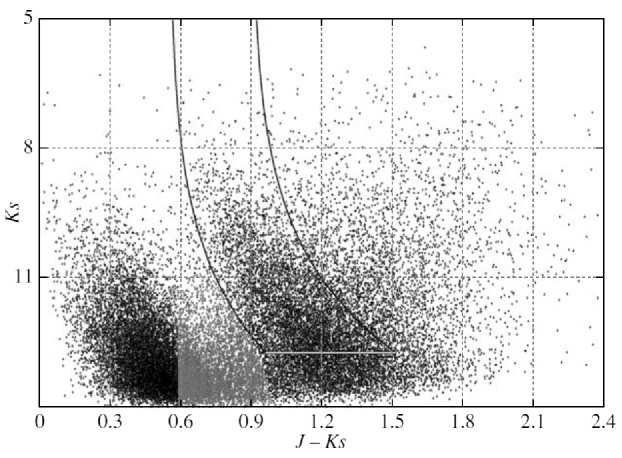
Figure 1: Distribution of the stars under consideration on the $(J-Ks)$ – $Ks$ diagram in the $2^{\circ}\times 2^{\circ}$ sky region centered at $l=100^{\circ}$, $b=0^{\circ}$. All stars in the region bounded by the curves and horizontal straight line were selected. The gray symbols mark the stars in the diagram region where red dwarfs of the same color as that of the selected clump giants dominate.

An example of the $(J-Ks)$ – $Ks$ diagram for the $2^{\circ}\times 2^{\circ}$ square of the sky centered at $b=0^{\circ}$ and $l=100^{\circ}$ is given in Fig. 1. The left cloud of stars consists of O-F main-sequence stars, the central cloud consists of clump giants, with the fraction of dwarfs being large among the faintest stars (the stars in the region of the diagram where the red dwarfs dominate are marked by the gray symbols), and the stars in the right part of the diagram are RGB ones. The selection boundaries derived for this square of the sky are indicated by two curves that are ultimately defined by Eqs. (1)–(5); more specifically, for the brightest stars with negligible extinction, they are defined by Eq. (4), while the shift of the curves along the horizontal axis with increasing $Ks$ depends on the coefficient $k$ and changes from one square of the sky to another. The white straight line at the bottom of the figure cuts off the diagram region where the clump giants are inseparable from the RGB stars and dwarfs, the sample of clump giants is incomplete, or the effects distorting the result are large.

The efficient of identifying the clump giants is explained by the following reasoning. We select the clump giants with $r<5$ kpc. At $M_{Ks}=-1.52^{m}$, we then have either (1) $A_{Ks}>0.2^{m}$ and $(J-Ks)>0.9^{m}$ or (2) $A_{Ks}<0.2^{m}$ and $Ks<12^{m}$. The dwarfs that can become an admixture because of their proximity to the Sun have $A_{Ks}\approx 0$ and $0.55^{m}<(J-Ks)<0.9^{m}$. Condition (1) is then reflected at the bottom of Fig. 1 – the reddening of giants does not allow them to be mixed with dwarfs because of different colors, while condition (2) is reflected in the middle part of the figure – the dwarfs with $M_{Ks}\approx 4.5^{m}$ at $Ks<12^{m}$ are within $r<300$ pc, while the number of dwarfs in this space is smaller than the number of clump giants within 5 kpc of the Sun approximately by one or two orders of magnitude.

The red dwarfs that fell into the sample were excluded as stars with large reduced proper motions $M^{\prime}_{Ks}=Ks-A_{Ks}+5+5\cdot~{}\lg(\mu)$, where $\mu=(\mu_{\alpha}\cos\delta^{2}+\mu_{\delta}^{2})^{1/2}$ is the total proper motion in arcseconds taken from the PPMXL catalogue (Roeser et al. 2010), where it is available for most of the stars considered. At $b=0^{\circ}$, the dwarfs revealed in this way account for less than 1% of the preselected stars. However, using $M^{\prime}_{Ks}$ turned out to be very important at $|b|=10^{\circ}$ (and, undoubtedly, extremely important at high latitudes): here, the admixture of dwarfs is about 10% and can apparently be revealed only by using the reduced proper motions.

Since the stars were selected using $(J-Ks)$, although the spatial variations of $E_{(J-H)}/E_{(H-Ks)}$ were analyzed by Zasowski et al. (2009), this analysis is distorted by strong selection effects and is not considered here.

In each square of the sky under consideration, we performed a moving calculation of the coefficients $E_{(H-W1)}/E_{(H-Ks)}$, $E_{(H-W2)}/E_{(H-Ks)}$, $E_{(H-W3)}/E_{(H-Ks)}$, $E_{(H-W4)}/E_{(H-Ks)}$ as a function of $r$ with an averaging window dependent on the star density in a given direction and varied in the range from 100 (toward the Galactic anticenter) to 300 (toward the Galactic center) stars. The stars are arranged by $r$ and the mean $\overline{r}$, along with the sought-for coefficients, is calculated for $100-300$ stars with minimum $r$. Then, we exclude the star with minimum $r$ from the set of stars under consideration, introduce the previously unused star with minimum $r$ instead of it, and repeat the calculations of $\overline{r}$ and the sought-for parameters. As a result, we obtain more than a thousand solutions including $\overline{r}$ with the corresponding set of sought-for coefficients for each square of the sky under consideration.

As has been pointed out above, the relative accuracy of individual $r$ determined by the scatter of individual $M_{Ks}$ about the mean is 15%. The relative accuracy of $\overline{r}$ is then $1-1.5\%$, i.e., given that the number of stars increases with distance in the solid angles under consideration, $15-60$ pc. Therefore, it is hoped that the variations of the coefficients under consideration in intervals larger than 60 pc are real.

RESULTS

The spatial variations of the coefficients $E_{(H-W1)}/E_{(H-Ks)}$, $E_{(H-W2)}/E_{(H-Ks)}$, $E_{(H-W3)}/E_{(H-Ks)}$ revealed here agree with those found by Zasowski et al. (2009) for the analogous coefficients $E_{(H-\lambda_{3.6})}/E_{(H-Ks)}$, $E_{(H-\lambda_{4.5})}/E_{(H-Ks)}$, $E_{(H-\lambda_{8.0})}/E_{(H-Ks)}$, although Zasowski et al. (2009) provide only the mean values of the coefficients for each longitude and, in addition, the ranges of distances considered by Zasowski et al. (2009) and in our study are different.

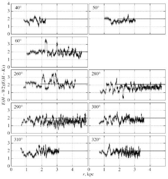
Figure 2: $E_{(H-W2)}/E_{(H-Ks)}$ versus heliocentric distance for longitudes of $40^{\circ}$, $50^{\circ}$, $60^{\circ}$, $260^{\circ}$, $280^{\circ}$, $290^{\circ}$, $300^{\circ}$, $310^{\circ}$, $320^{\circ}$ (black curves with gray error bands) in comparison with the analogous results from Zasowski et al. (2009) (horizontal straight lines).

As an example, Fig. 2 shows the variations of $E_{(H-W2)}/E_{(H-Ks)}$ with heliocentric distance for longitudes of $40^{\circ}$, $50^{\circ}$, $60^{\circ}$, $260^{\circ}$, $280^{\circ}$, $290^{\circ}$, $300^{\circ}$, $310^{\circ}$, $320^{\circ}$ (black curves with gray error bands) in comparison with the mean coefficient $E_{(H-\lambda_{4.5})}/E_{(H-Ks)}$ from Zasowski et al. (2009) (horizontal straight lines; the accuracy of the mean result by Zasowski et al. (2009) is approximately the thickness of these straight lines). Comparison for longitudes of $20^{\circ}$, $30^{\circ}$, $90^{\circ}$, $270^{\circ}$, $330^{\circ}$, $340^{\circ}$ is given in other figures. We see that some of the variations in coefficient are significant and seem to correspond to large Galactic structures, most likely spiral arms. We also see that, despite the variations in an interval of tens and hundreds of pc, there are no systematic $E_{(H-W2)}/E_{(H-Ks)}$ trends in an interval of several kpc at these longitudes in the $W2$ band.

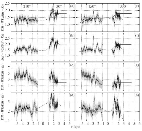
Figure 4: Same as Fig. 3 for longitudes of $210^{\circ}$ (negative $r$) and $30^{\circ}$ (positive $r$) (a–d), $150^{\circ}$ (negative r) and $330^{\circ}$ (positive r) (e–h).

In Fig. 3, the coefficients $E_{(H-W1)}/E_{(H-Ks)}$, $E_{(H-W2)}/E_{(H-Ks)}$, $E_{(H-W3)}/E_{(H-Ks)}$, $E_{(H-W4)}/E_{(H-Ks)}$ are plotted against the heliocentric distance for longitudes of $200^{\circ}$ (negative $r$) and $20^{\circ}$ (positive $r$) (Figs. 3a–3d), $160^{\circ}$ (negative $r$) and $340^{\circ}$ (positive $r$) (Figs. 3e–3h)) (black curves with gray error bands) in comparison with the analogous results from Zasowski et al. (2009) (horizontal straight lines; the accuracy of the mean is approximately the thickness of these straight lines). Figure 4 shows analogous results for longitudes of $210^{\circ}$ (negative $r$) and $30^{\circ}$ (positive $r$) (Figs. 4a 4d), $150^{\circ}$ (negative $r$) and $330^{\circ}$ (positive $r$) (Figs. 4e–4h). These longitudes were selected among all of those considered as being closest to the direction to the Galactic center ($20^{\circ}$, $30^{\circ}$, $330^{\circ}$ and $340^{\circ}$) and oppositely directed with respect to them ($200^{\circ}$, $210^{\circ}$, $150^{\circ}$ and $160^{\circ}$, respectively).

The minima in the curves shown in the figure correspond to a larger fraction of dust grains with sizes of about 3, 4, 10, and 20 microns than that of dust grains with a size of about 2 microns for $E_{(H-W1)}/E_{(H-Ks)}$, $E_{(H-W2)}/E_{(H-Ks)}$, $E_{(H-W3)}/E_{(H-Ks)}$, $E_{(H-W4)}/E_{(H-Ks)}$, respectively, or other dust properties causing a higher extinction of radiation with a longer wavelength. In contrast, the maxima in the curves correspond to a larger amount of fine dust if precisely the dust grain size is a characteristic determining the extinction.

In Figs. 3 and 4, just as in Fig. 2, we see agreement of our results with those from Zasowski et al. (2009). In addition, there is a clear correlation between the results in the $W1$ and $W2$ bands and their slight deviation from those in the $W4$ and particularly $W3$ bands.

For $W4$, this discrepancy is due to a large deviation of the wavelength from the $W1$ and $W2$ bands. This leads us to conclude that the fraction of dust grains about 20 microns in size represented by the coefficient $E_{(H-W4)}/E_{(H-Ks)}$ and their spatial distribution correlate weakly with those for dust grains about 3 and 4 microns in size.

The results for the $W3$ band differ from the remaining ones, because there is a well-known broad absorption line with $\lambda=9.7$ microns in this band produced by amorphous silicates contained in the dust. Indebetouw et al. (2005) and Zasowski et al. (2009) discussed this effect for the Spitzer-IRAC $\lambda=8$ microns band and showed an insignificant manifestation of this effect for shorter-wavelength bands. The absence of a correlation between the results for $W3$ and $W4$ in our study shows that this effect apparently does not manifest itself at $\lambda>20$ microns either. In the $W3$ band in Figs. 3 and 4, we see a systematic trend of the curves absent for the $W1$, $W2$, and $W4$ bands. This trend is consistent for all four longitudes under consideration and exhibits a minimum of $E_{(H-W3)}/E_{(H-Ks)}$ within the nearest kiloparsec. Since the data acquisition and reduction procedure in all bands is the same, this trend seems to be not an artifact but a manifestation of a peculiar distribution and/or properties of the dust responsible for the extinction in the $W3$ band. Given the probable connection of this extinction with amorphous silicates, it can be hypothesized that, in contrast to the remaining coefficients, the spatial variations of $E_{(H-W3)}/E_{(H-Ks)}$ seen in the figures are caused not by variations of the dust grain size distribution but by variations of the dust mean chemical composition.

For all of the longitudes under consideration, except perhaps $160^{\circ}$ and $340^{\circ}$ (Fig. 3h), the same systematic trend of the curves approximately illustrated by the dashed curves can be seen in the $W1$, $W2$, and $W4$ bands: as one recedes from the Galactic center, the curves reach a global maximum near $r\approx 1-2$ kpc (slightly closer to the Sun in $W4$ than in $W1$ and $W2$) and in this part they agree with the results from Zasowski et al. (2009), but still farther from the Galactic center, despite the local maxima and minima, the coefficients under consideration tend to decrease (i.e., the gray extinction in the solar neighborhood is minimal). If the spatial variations of the coefficients under consideration are caused by variations of the dust grain size distribution, then this systematic trend shows a decrease in the fraction of coarse dust with increasing Galactocentric distance in the inner (relative to the Sun) Galaxy (the same conclusion for the same region was reached by Zasowski et al. (2009)) and a decrease in this fraction in the outer Galaxy.

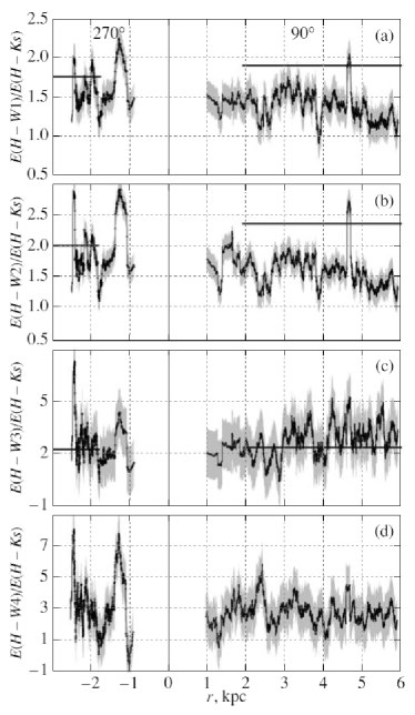
Figure 5: Same as Fig. 3 for longitudes of $270^{\circ}$ (negative $r$) and $90^{\circ}$ (positive $r$).

The global extrema and trends are less prominent in Fig. 5, where results similar to those in Fig. 3 are shown, but for longitudes of $270^{\circ}$ (negative $r$) and $90^{\circ}$ (positive $r$): the results for $W3$ have a minimum within the nearest kiloparsec here as well, while for a longitude of $90^{\circ}$, there is a noticeable decrease in $E_{(H-W1)}/E_{(H-Ks)}$ and $E_{(H-W2)}/E_{(H-Ks)}$ with increasing heliocentric distance, especially farther than 5 kpc, although both effects are less pronounced than in Figs. 3 and 4. The results for adjacent longitudes in the $W2$ band presented in Figs. 2c–2f show no clear extrema and trends, although the trends will possibly manifest themselves farther than 5 kpc from the Sun for all these longitudes, just as for $l=90^{\circ}$. Our results for $l=90^{\circ}$ in the $W1$ and $W2$ bands, on average, differ markedly from those from Zasowski et al. (2009). However, this is the only longitude with such a difference and, in addition, the result from Zasowski et al. (2009) for $l=90^{\circ}$ differs from their results for all the remaining longitudes.

Significant rises and falls of all coefficients are clearly seen at a longitude of $270^{\circ}$, in which the dustrich regions of the local spiral arm seem to manifest themselves. In any case, the extinction begins to sharply increase at this longitude at a distance of more than 1 kpc. This can be seen when analyzing the corresponding $(J-Ks)$ – $Ks$ diagram: $A_{Ks}\approx 0.7^{m}$ already at a heliocentric distance of 2.5 kpc, i.e., $A_{V}\approx 7^{m}$, according to Eqs. (3). High extinction begins to hide clump giants, and the sample becomes incomplete. Therefore, no reliable results have been obtained farther than 2.5 kpc from the Sun for a longitude of $270^{\circ}$.

Thus, the global extrema of the coefficients under consideration manifest themselves at certain Galactocentric distances, within $\pm 3$ kpc of the Sun s Galactocentric distance. The Galactic disk at these Galactocentric distances differs from the remaining space of the Galaxy primarily by the great role of the spiral arms that are absent at the Galactic center, at the disk edge, and outside the disk.

Figure 6 shows the same as in Figs. 3–5 but for the squares of the sky centered at $l=180^{\circ}$, $b=0^{\circ}$ (black curves, negative $r$), $l=180^{\circ}$, $b=+10^{\circ}$ (gray solid curves, negative $r$), $l=180^{\circ}$, $b=-10^{\circ}$ (gray dashed curves, negative $r$), $l=340^{\circ}$, $b=0^{\circ}$ (black curves, positive $r$), $l=340^{\circ}$, $b=+10^{\circ}$ (gray solid curves, positive $r$), $l=340^{\circ}$, $b=-10^{\circ}$ (gray dashed curves, positive $r$). We see that the variations of $E_{(H-W1)}/E_{(H-Ks)}$ and $E_{(H-W2)}/E_{(H-Ks)}$ change qualitatively even at a small distance from the Galactic plane: toward both the Galactic center and anticenter, both above and below the Galactic plane, these coefficients are systematically much smaller than those in the plane itself, although the curves approach each other toward the Galactic anticenter. If precisely the dust grain size is a characteristic determining the extinction law, then we see that the fraction of fine dust in the Galactic plane is maximal (or the mean dust grain size is minimal), but the fraction of coarse dust (or the mean grain size) increases with distance from the plane. Where the finest dust is observed in the plane, the fraction of coarse dust outside the plane is particularly large: the black and gray curves anticorrelate with each other in many places.

In the inner (relative to the Sun) Galaxy (positive $r$ in the figures), the difference between the dust grain sizes in and outside the Galactic plane also manifests itself for $E_{(H-W3)}/E_{(H-Ks)}$ and $E_{(H-W4)}/E_{(H-Ks)}$.

Sharp drops of the curves at $r\approx-1$ kpc and $r\approx-2.8$ kpc are clearly seen in Figs. 3a, 3b, 3d–3f, 3h, 4a, 4b, 4e, 4f, and 4h. These apparently show the positions and influence of spiral arms, respectively, the Perseus arm and the more distant outer arm. Different arms seem to have also manifested themselves in the same way on other graphs, but, in many cases, an improper perspective or errors in the distances of stars smooth out their manifestation. We see that, in most cases, at a sharp drop of the curve, its minimum is farther from the Galactic center than its maximum. Thus, coarser dust dominates in the outer (relative to the Galactic center) part of the arm, while fine dust dominates in its inner part. This is an expected result for a twisting spiral pattern with a leading arm edge: an increase in the density of the interstellar medium and other processes at the outer edge lead to intense sticking of dust grains, while supernova explosions and other processes deep in the arm destroy the dust grains. Thus, the disk at Galactocentric distances of $4-12$ kpc (if the Sun is 8 kpc away from the Galactic center), where the spiral pattern exists, is a Galactic region (possibly the only one) where the dust is sorted by size and is fragmented significantly. This “dust sorting and fragmentation factory” apparently does not work where there is no spiral pattern, i.e., near the Galactic center (as was shown by Zasowski et al. 2009), at the disk edge (farther than 5 kpc from the Sun toward the Galactic anticenter, according to Figs. 6a and 6b), and outside the disk (gray curves in Figs. 6a and 6b). In all these regions outside the spiral pattern, the dust grain size distribution must then be the same, constant, and noticeably different from that in the solar neighborhood apparently in favor of coarse dust grains. This will be verified in our subsequent study of the extinction law and related dust properties outside the Galactic disk using 2MASS and WISE data.

CONCLUSIONS

This study showed the possibility of using the new WISE catalogue, along with the 2MASS catalogue, to analyze the interstellar dust properties and the corresponding variations of the IR extinction law based on multicolor IR photometry in the range from 1 to 27 microns for millions of stars over the entire sky. Owing to the high accuracy of the photometric data and the very large number of stars used, the classical method of extrapolation of the extinction law applied to clump giants is operable. The coefficients $E_{(H-W1)}/E_{(H-Ks)}$, $E_{(H-W2)}/E_{(H-Ks)}$, $E_{(H-W3)}/E_{(H-Ks)}$ and $E_{(H-W4)}/E_{(H-Ks)}$ obtained in this method are good characteristics of the extinction law and dust properties near the Galactic plane, although the analogous coefficients using $E_{(J-H)}$ instead of $E_{(H-Ks)}$ are also informative in the second and third quadrants.

It turned out that the spatial variations of these coefficients for the $W1$ and $W2$ bands correlate with one another and usually differ slightly from those for the $W4$ band and markedly for the W3 band. The results for the $W3$ band differing from the remaining ones seem to be affected by the absorption by amorphous silicates at a wavelength of 9.7 microns and, in contrast to the remaining bands, seem to reflect the variations of the mean chemical composition rather than the dust grain size to a greater extent.

Our results agree with those obtained by Zasowski et al. (2009) using 2MASS and Spitzer-IRAC photometry for the same longitudes and similar photometric bands, confirming the main result by Zasowski et al. (2009): in the inner (relative to the Sun) Galactic disk, the fraction of fine dust increases with Galactocentric distance (or the mean dust grain size decreases). However, in the outer Galactic disk that was not considered by Zasowski et al. (2009), this trend is reversed: at the disk edge, the fraction of coarse dust is larger than that in the solar neighborhood. This general Galactic trend seems to be explained by the influence of the spiral pattern: its processes sort the dust by size and fragment it so that coarse and fine dust tend to accumulate, respectively, at the inner and outer (relative to the Galactic center) edges of the spiral arms. As a result, fine dust may exist only in the part of the Galactic disk far from both the Galactic center and the edge, while the fraction of fine dust at the Galactic center, the disk edge, and outside the disk is minimal.

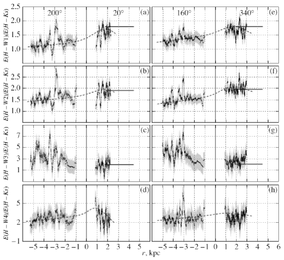
Figure 3: $E_{(H-W1)}/E_{(H-Ks)}$, $E_{(H-W2)}/E_{(H-Ks)}$, $E_{(H-W3)}/E_{(H-Ks)}$, $E_{(H-W4)}/E_{(H-Ks)}$ versus heliocentric distance for longitudes of $200^{\circ}$ (negative $r$) and $20^{\circ}$ (positive $r$) (a–d), $160^{\circ}$ (negative $r$) and $340^{\circ}$ (positive $r$) (e–h) (black curves with gray error bands). The horizontal straight lines indicate the analogous results from Zasowski et al. (2009). The dashed lines indicate the systematic variations of the coefficients.

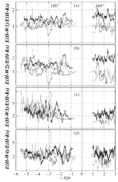
Figure 6: Same as Fig. 3 for $l=180^{\circ}$, $b=0^{\circ}$ (black curves, negative $r$), $l=180^{\circ}$, $b=+10^{\circ}$ (gray solid curves, negative $r$), $l=180^{\circ}$, $b=-10^{\circ}$ (gray dashed curves, negative $r$), $l=340^{\circ}$, $b=0^{\circ}$ (black curves, positive $r$), $l=340^{\circ}$, $b=+10^{\circ}$ (gray solid curves, positive $r$), $l=340^{\circ}$, $b=-10^{\circ}$ (gray dashed curves, positive $r$).

References

- 1. R.A. Benjamin, E. Churchwell, B.L. Babler, et al., Publ. Astron. Soc. Pacif. 115, 953 (2003).
- 2. G. Bertelli, L. Girardi, P. Marigo, et al., Astron. Astrophys. 484, 815 (2008).
- 3. J.A. Cardelli, G.C. Clayton and J.S. Mathis, Astrophys. J. 345, 245 (1989).
- 4. B.T. Draine, Ann. Rev. Astron. Astrophys. 41, 241 (2003).
- 5. R. Drimmel, A. Cabrera-Lavers and M. Lopez-Corredoira, Astron. Astrophys. 409, 205 (2003).
- 6. ESA, Hipparcos and Tycho catalogues (ESA, 1997).
- 7. P.C. Frisch, J.M. Dorschner, J. Geiss, et al., Astrophys. J. 525, 492 (1999).
- 8. G.A. Gontcharov, Astron. Lett. 34, 785 (2008).
- 9. G.A. Gontcharov, Astron. Lett. 35, 638 (2009a).
- 10. G.A. Gontcharov, Astron. Lett. 35, 780 (2009b).
- 11. G.A. Gontcharov, Astron. Lett. 36, 584 (2010).
- 12. G.A. Gontcharov, Astron. Lett. 38, 12 (2012a).
- 13. G.A. Gontcharov, Astron. Lett. 38, 87 (2012b).
- 14. M.A.T. Groenewegen, Astron. Astrophys. 488, 935 (2008).
- 15. E. Høg, C. Fabricius, V.V. Makarov, et al., Astron. Astrophys. 355, L27 (2000).
- 16. R. Indebetouw, J.S. Mathis, B.L. Babler, et al., Astrophys. J. 619, 931 (2005).
- 17. H.L. Jonhson and J. Borgman, Bull. Astron. Inst. Netherlands 17, 115 (1963).
- 18. H. Krüger, E. Grün, M. Landgraf, et al., Planet. Space Sci. 49, 1303 (2001).
- 19. F. van Leeuwen, Astron. Astrophys. 474, 653 (2007).
- 20. M. Lopez-Corredoira, A. Cabrera-Lavers, F. Garzon, et al., Astron. Astrophys. 394, 883 (2002).
- 21. P. Marigo, L. Girardi, A. Bressan, et al., Astron. Astrophys. 482, 883 (2008).
- 22. D.J. Marshall, A.C. Robin, C.Reyle, et al., Astron. Astrophys. 453, 635 (2006).
- 23. S. Nishiyama, M. Tamura, H.Hatano, et al., Astrophys. J. 696, 1407 (2009).
- 24. W. Reis and W.J.B. Corradi, Astron. Astrophys. 486, 471 (2008).
- 25. S. Roeser, M. Demleitner and E. Schilbach, Astron. J. 139, 2440 (2010).
- 26. W. Skorzynski, A. Strobel and G. Galazutdinov, Astron. Astrophys. 408, 297 (2003).
- 27. M.F. Skrutskie, R.M. Cutri, R. Stiening, et al., Astron. J. 131, 1163 (2006); http://www.ipac.caltech.edu/2mass/releases/allsky/index.html.
- 28. J.C. Weingartner and B.T. Draine, Astrophys. J. 548, 296 (2001).
- 29. E.L. Wright, P.R.M. Eisenhardt, A.K. Mainzer et. al., Astron. J. 140, 1868 (2010), http://irsa.ipac.caltech.edu/Missions/wise.html
- 30. G. Zasowski, S.R. Majewski, R. Indebetouw, et al., Astrophys. J. 707, 510 (2009).