Spatio-temporal interference of photo electron wave packets and time scale of non-adiabatic transition in high-frequency regime

Abstract

The method of the envelope Hamiltonian [K. Toyota, U. Saalmann, and J. M. Rost, New J. Phys. 17, 073005 (2015)] is applied to further study a detachment dynamics of a model negative ion in one-dimension in high-frequency regime. This method is based on the Floquet approach, but the time-dependency of an envelope function is explicitly kept for arbitrary pulse durations. Therefore, it is capable of describing not only a photo absorption/emission but also a non-adiabatic transition which is induced by the time-varying envelope of the pulse. It was shown that the envelope Hamiltonian accurately retrieves the results obtained by the time-dependent Schrödinger equation, and underlying physics were well understood by the adiabatic approximation based on the envelope Hamiltonian. In this paper, we further explore two more aspects of the detachment dynamics, which were not done in our previous work. First, we find out features of both a spatial and temporal interference of photo electron wave packets in a photo absorption process. We conclude that both the interference mechanisms are universal in ionization dynamics in high-frequency regime. To our knowledge, it is first time that both the interference mechanisms in high-frequency regime are extracted from the first principle. Second, we extract a pulse duration which maximize a yield of the non-adiabatic transition as a function of a pulse duration. It is shown that it becomes maximum when the pulse duration is comparable to a time-scale of an electron.

I Introduction

The latest experimental techniques of high order harmonic generations can generate coherent light sources in soft x-ray range CA , and opened up the new realm of the research area so-called high-frequency regime. Here the terminology “high-frequency” means that a photon energy is high enough to ionize a ground state electron by single photon absorption. Meanwhile, high-frequency regime has been intensively studied in theory more than three decades in terms of the high-frequency Floquet theory (HFFT) for monochromatic laser fields developed by Gavrila and Kaminski GK . The HFFT is developed in the Kramers-Henneberger (KH) frame Henne . In the KH frame, an effect of the laser field is described by an atomic potential quivering along a classical trajectory of a free electron in the laser fields. This is called the KH potential. In high-frequency limit, where the single optical cycle of the laser field is much shorter than the electron’s time scale, it was shown that all the Fourier components of the KH potential can be ignored except the zeroth component i.e. a time average of the KH potential GK . This is often called the dressed potential. All the other photon absorption/emission channels then can be treated perturbatively for bound states of the dressed potential even these amplitudes are comparable with the dressed potential.

After the foundation of the HFFT, a lot of literatures have been involved to study ionization dynamics in high-frequency regime. One of the most striking physical phenomenon in high-frequency regime is the stabilization, which an ionization rate begins to decrease for an intensity higher than a certain critical value, first found by Pont and Gavrila PG . A great number of literatures had been devoted to understand this counter-intuitive phenomenon. You et al. YM showed that the stabilization stems from a spatial interference of photo electron wave packets launched at two turning points of the classical electron in laser fields. For small values of its quiver amplitude, the interference is constructive because they are produced almost the same positions in space. However, this picture turns into destructive for a quiver amplitude larger than a certain critical value. This is the origin of the stabilization.

The HFFT has given us interesting physical insights in high-frequency regime, but it can only be applied for monochromatic laser fields i.e. infinite pulse duration. However, laser pulses of attosecond time scale has become available in the latest experiments as mentioned above. These unprecedented laser pulses will be employed to study light-matter interactions in extremely short time scale in high-frequency regime, where effects of a time-varying envelope function of a pulse is expected to play important roles. Therefore, it is highly desirable to develop theoretical methods in high-frequency regime to adequately treat finite pulse duration beyond the HFFT.

Under such circumstances, we developed the envelope Hamiltonian to treat photo ionization dynamics in high-frequency regime in our previous work TS . Photo electron amplitudes were analytically derived in the framework of the adiabatic approximation based on the envelope Hamiltonian. The procedures follows the HFFT i.e. we realize a dressed potential and treat photon absorption/emission channels perturbatively but the time-dependency of a pulse envelope is explicitly remained. Thus we also obtain the photo electron amplitudes for a non-adiabatic transition induced by the time-dependent envelope function which does not show up in the original HFFT. The capability of the envelope Hamiltonian and the adiabatic approximation were demonstrated in TS utilizing a simple model in one dimension in the stabilization regime. It was shown that the results obtained by the full time-dependent Schrödinger equation (TDSE) calculations were accurately reconstructed by the TDSE for the envelope Hamiltonian.

In this paper, we further explore ionization dynamics in high-frequency regime working on two subjects utilizing the envelope Hamiltonian. First, we revisit the oscillating substructure in photon absorption peaks in high-frequency regime, which has been recently studied by several groups TT ; DC ; YF ; YMad . In TT , they found the oscillating structure in the stabilization regime, and reconstructed it taking into account a spatial and temporal interference of photo electron wave packets. In the stabilization regime, ionization probability as a function of time has two peaks before and after a peak intensity due to the spatial interference of photo electron wave packets. This means that a photo electron wave packet of a certain energy is created in a rising and falling part of a pulse, and they provoke the temporal interference whose phase difference is given by different moments of their birth in time. However, their formulas were obtained in an empirical way incorporating a quasi static picture into the HFFT. On the other hand, in DC ; YF ; YMad , they only addressed the temporal interference although their theoretical approach was based on the first principle. We consider that they did not need to take into account the spatial interference because their maximum quiver amplitude of a free electron in their pulse was below a threshold for the emergence of the stabilization. In this paper, to our knowledge, we find out for the first time both the signature of the spatial and temporal interference in the formula obtained from the first principle.

The second subject in this paper is to extract an optimal pulse duration to maximize a yield of the non-adiabatic transition. It is found that the yield as a function of a pulse duration has a maximum at a certain pulse duration in our previous work TS . We find out a formula to predict the peak position, and show that the yield becomes maximum when the pulse duration is close to a time scale of an electron. As far as we know, these two subjects have not been explored yet in high-frequency regime due to the lack of appropriate theoretical frameworks which can take into account time-varying envelope functions. So, we strongly believe that these are worth to gain further insights for ionization dynamics in high-frequency regime.

This paper is thus organized as follows. In Sec. II, we introduce our theoretical methods. We briefly summarize the formulations in TS for a case of one dimension to refer them in later. In Sec. IIA, B, and C, we derive the envelope Hamiltonian in the KH frame employing a normalized classical trajectory. In Sec. IID, we derive photo electron amplitudes for the photon adsorption/emission processes and non-adiabatic transition. After considering on the non-adiabatic transition in Sec. II.5, we extract the evidence of the spatial and temporal interference in the formula of the photon absorption spectrum with the aid of the saddle point method in Sec. II.6. In Sec. III, we study a detachment dynamics of a model negative ion in high-frequency regime to demonstrate our theory. In Sec. III.1, we revisit the oscillating structure in photon absorption peaks to confirm that our theory is consistent with previously known results TT ; DC ; YF ; YMad . In Sec. III.2, we find out an optimal pulse duration to maximize a yield of non-adiabatic transition. In Sec. IV, we conclude the paper with future perspectives. Atomic units are used thorough out the paper.

II Theoretical methods

In this section, we summarize our theoretical method TS in one dimension to refer them in later.

II.1 TDSE in the Kramers-Henneberger frame

The time-dependent Schrödinger equation in one dimension reads,

$$H(t)|\Psi(t)\rangle=i\frac{\partial}{\partial t}|\Psi(t)\rangle.$$ (1)

The Hamiltonian $H(t)$ within dipole approximation in the Kramers-Henneberger (KH) frame is given by

$$H(t)=-\frac{1}{2}\frac{\partial^{2}}{\partial x^{2}}+V(x+x_{\omega}(t)),$$ (2)

where $V(x)$ is an atomic potential. The function $x_{\omega}(t)$ represents a classical trajectory of a free electron in a laser pulse $F(t)$,

$$\frac{d^{2}x_{\omega}}{dt^{2}}=-F(t).$$ (3)

The laser pulse $F(t)$ satisfies

$$\lim_{t\to\pm\infty}F(t)=0,$$ (4a)

$$\int_{-\infty}^{\infty}F(t^{\prime})dt^{\prime}=0.$$ (4b)

In the KH frame, external fields are described by quivering motions of the atomic potential along the classical trajectory Eq. (3), and this potential is called the KH potential.

II.2 Normalized classical trajectory

We define the classical trajectory $x_{\omega}(t)$ in Eq. (2) as

$$x_{\omega}(t)=\alpha(t)\cos(\omega t+\delta).$$ (5)

Then the pulse is given by Eq. (3). The function $\alpha(t)$ is the envelope of the pulse given by

$$\alpha(t)=\alpha_{0}e^{-a\left(\frac{t}{T}\right)^{2}}$$ (6)

where $a=2\log(2)$ so that a pulse duration $T$ is defined by the full width of half maximum (FWHM) of $F^{2}(t)$. The constant $\alpha_{0}$ is given by

$$\alpha_{0}=\frac{F_{0}}{\omega^{2}+\frac{2a}{T^{2}}}$$ (7)

so that the peak field amplitude becomes $F(0)=F_{0}\cos\delta$. Note that our pulse $F(t)$ defined in this way satisfies the conditions Eqs. (4). In this paper, we consider values of a photon energy $\omega$ much higher than an ionization potential of an ground state,

$$\omega\gg I_{p}.$$ (8)

II.3 The envelope Hamiltonian

For a given value of the pulse envelope $\alpha(t)$, Eq. (6), we introduce the function $V_{n}(x,t)$,

$$V_{n}(x,t)=\frac{1}{T_{\omega}}\int_{0}^{T_{\omega}}V(x+\alpha(t)\cos(\omega t^{\prime}+\delta))e^{in\omega t^{\prime}}dt^{\prime}.$$ (9)

Let us consider how many functions $V_{n}(x,t)$ are needed to reconstruct the KH potential. First, we consider a short pulse limit $T\to 0$. In this case, the value of the envelope Eq. (6) is very small; see Eq. (7). So, considering the Taylor expansion of the function $V_{n}(x,t)$ for $n=0,~{}\pm 1~{}$ and $\pm 2$ up to the order of $\alpha^{2}(t)$,

$$V_{0}(x,t) \approx V(x)+\frac{1}{4}V^{\prime\prime}(x)\alpha^{2}(t),$$ (10a)

$$V_{\pm 1}(x,t) \approx \frac{1}{2}V^{\prime}(x)\alpha(t)e^{\mp i\delta},$$ (10b)

$$V_{\pm 2}(x,t) \approx \frac{1}{8}V^{\prime\prime}(x)\alpha^{2}(t)e^{\mp 2i\delta}.$$ (10c)

Here the prime represents spatial derivative. We then obtain

$$\sum_{n=-2}^{2}V_{n}(x,t)e^{-in\omega t}=V(x+x_{\omega}(t))+O(\alpha^{3}(t)).$$ (10d)

Second, we consider a long pulse limit $$T\to\infty \alpha(t) t V_{n}(x,t)$$. In this case, the envelope function Eq. (6) varies slowly in time since a lot of optical cycles are contained in the pulse. So, we can define the momentary Fourier expansion of the KH potential for a given time using the function Eq. (9),

$$V(x+x_{\omega}(t))=\sum_{n=-\infty}^{\infty}V_{n}(x,t)e^{-in\omega t}.$$ (10e)

This expression is exact for the long pulse limit $T\to\infty$. Since we work on high-frequency regime characterized by the inequality Eq. (8), it is enough to only consider the above summation $|n|\leq 2$.

Having confirmed that the KH potential can be accurately approximated using a few terms of the function $V_{n}(x,t)$ for both the opposite time scale $T\to 0$ and $T\to\infty$, we introduce the envelope Hamiltonian $H_{\rm env}(t)$

$$H_{\rm env}(t)=H_{0}(t)+U(x,t),$$ (11)

where $H_{0}(t)$ and $U(x,t)$ are defined by

$$H_{0}(t) = -\frac{1}{2}\frac{\partial^{2}}{\partial x^{2}}+V_{0}(x,t),$$ (12a)

$$U(x,t) = \sum_{n=\pm 1,\pm 2}V_{n}(x,t)e^{-in\omega t}$$ (12b)

and we consider the TDSE for $H_{\rm env}(t)$,

$$H_{\rm env}(t)|\psi(t)\rangle=i\frac{\partial}{\partial t}|\psi(t)\rangle.$$ (13)

We call this equation the envelope TDSE. In the above, we separated the function $V_{0}(x,t)$ from Eq. (10e), and used it to construct the quantity $H_{0}(t)$, Eq. (12a). The function $H_{0}(t)$ in Eq. (12a) reduces to the atomic Hamiltonian for $t\to\pm\infty$. So, it is considered that the quantity $H_{0}(t)$ represents a distorted Hamiltonian of the electron during the action of the pulse. It is often called the dressed Hamiltonian. The equivalent Hamiltonian for the case of monochromatic fields was also considered by Henneberger in Henne . In the paper, he pointed out that a fast convergence of a photo ionization cross section in a strong field can be achieved in perturbation theory based on $H_{0}(t)$, since all the orders of the field amplitude $F_{0}$ are included in its eigen function and eigen energy.

II.4 Adiabatic approximation for photo ionization

In this subsection, we implement an adiabatic approximation for photo electron amplitudes. We derive photo electron amplitudes in one-dimension based on the envelope Hamiltonian, Eq. (11), to utilize them in later sections. The full derivations with an arbitrary number of bound states in three dimension are found in TS . Let $|0(t)\rangle$ and $|k,t\rangle$ be a ground state and scattering state of the dressed Hamiltonian $H_{0}(t)$ Eq. (12a),

$$H_{0}(t)|0(t)\rangle = E_{0}(t)|0(t)\rangle,$$ (14a)

$$H_{0}(t)|k,t\rangle = E|k,t\rangle,$$ (14b)

where

$$E=\frac{k^{2}}{2}.$$ (15)

The orthogonality is

$$\langle 0(t)|0(t)\rangle = 1,$$ (16a)

$$\langle k,t|k^{\prime},t\rangle = 2\pi\delta(k-k^{\prime}).$$ (16b)

Employing them, we expand the solution of the envelope TDSE Eq. (13),

$$|\psi(t)\rangle=e^{-i\chi(t)}\left[C_{0}(t)|0(t)\rangle e^{-i\int_{-\infty}^{t}E_{0}(t^{\prime})dt^{\prime}}+\int_{-\infty}^{\infty}C_{k^{\prime}}(t)|k^{\prime},t\rangle e^{-iE^{\prime}t}\frac{dk^{\prime}}{2\pi}\right],$$ (17)

where $E^{\prime}=k^{\prime 2}/2$ and the coefficients $C_{0}(t)$ and $C_{k}(t)$ represent the ground state population and photo electron amplitude of momentum $k$ for a certain time $t$, respectively. The phase $\chi(t)$ is given by

$$\chi(t)=\int_{-\infty}^{t}\langle 0(t^{\prime})|U(x,t^{\prime})-i\frac{\partial}{\partial t^{\prime}}|0(t^{\prime})\rangle dt^{\prime},$$ (18)

so that coupled differential equations for the coefficients $C_{0}(t)$ and $C_{k}(t)$ become simple. Let us introduce the notation

$$\Phi_{n}(t)=-\int_{-\infty}^{t}E_{0}(t^{\prime})dt^{\prime}-n\omega t+Et.$$ (19)

Substituting the expansion Eq. (17) into the envelope TDSE Eq. (13), we obtain

$$i\frac{dC_{0}}{dt} = e^{i\int_{-\infty}^{t}E_{0}(t^{\prime})dt^{\prime}}\int_{-\infty}^{\infty}Q_{0k^{\prime}}(t)C_{k^{\prime}}(t)e^{-iE^{\prime}t}\frac{dk^{\prime}}{2\pi},$$ (20a)

$$i\frac{\partial C_{k}}{\partial t} = Q_{k0}(t)C_{0}(t)e^{i\Phi_{0}(t^{\prime})}+\int_{-\infty}^{\infty}Q_{kk^{\prime}}(t)C_{k^{\prime}}(t^{\prime})e^{-i(E^{\prime}-E)t}\frac{dk^{\prime}}{2\pi},$$ (20b)

where

$$Q_{k0}(t)=\langle k,t|U(x,t)-i\frac{\partial}{\partial t}|0(t)\rangle,~{}{\rm etc}.$$ (20c)

Using the Hellmann-Feynman theorem, the quantity $$Q_{k0}(t)$$ becomes

$$Q_{k0}(t)=\langle k,t|U(x,t)+i\frac{\dot{V}_{0}(x,t)}{E-E_{0}(t)}|0(t)\rangle,$$ (20d)

where $\dot{V}_{0}$ is time derivative of $V_{0}$. Eqs. (20) can be solved perturbatively. Let us assume the zeroth order solution as $C_{0}^{(0)}(t)=1$ and $C_{k}^{(0)}(t)=0$. Then the first order solution is given by

$$C_{0}^{(1)}(t) = 1,$$ (21a)

$$C_{k}^{(1)}(t) = -i\int_{-\infty}^{t}Q_{k0}(t^{\prime})e^{i\Phi_{0}(t^{\prime})}dt^{\prime}$$ (21b)

The photo electron spectrum $dp/dk$ is thus approximated as,

$$\frac{dp}{dk}\simeq\left|\lim_{t\to\infty}C_{k}^{(1)}(t)\right|^{2}=\left|\sum_{n=-2}^{2}C^{(1)}_{n\omega}(k)\right|^{2}.$$ (22)

The function $C_{n\omega}^{(1)}(k)$ is defined by

$$C_{n\omega}^{(1)}(k)=\int_{-\infty}^{\infty}M_{n\omega}(k,t)e^{i\Phi_{n}(t)}dt,$$ (23a)

where

$$M_{n\omega}(k,t)=\left\{\begin{array}[]{cr}\langle k,t|i\frac{\dot{V}_{0}(x,t)}{E-E_{0}(t)}|0(t)\rangle&(n=0),\\ \langle k,t|V_{n}(x,t)|0(t)\rangle&(n\neq 0).\end{array}\right.$$ (23b)

The total ionization yield is given by

$$P_{\rm ion}=\int_{-\infty}^{\infty}\left|\sum_{n=-2}^{2}C^{(1)}_{n\omega}(k)\right|^{2}\frac{dk}{2\pi}.$$ (24)

The ionization yield by each channel is given by

$$P_{n}=\int_{-\infty}^{\infty}|C^{(1)}_{n\omega}(k)|^{2}\frac{dk}{2\pi}.$$ (25)

II.5 Non-adiabatic transition

The total photo electron amplitude Eq. (23a) consists of two different kinds of physical processes. The first one is given by $n=0$ in Eq. (23b) which represents the non-adiabatic transitions to the continuum induced by the time-dependency of the ground state $|0(t)\rangle$. Therefore, one speculates that the following TDSE is responsible for the non-adiabatic transition,

$$H_{0}(t)|\psi_{0}(t)\rangle=i\frac{\partial}{\partial t}|\psi_{0}(t)\rangle.$$ (26)

The TDSE Eq. (26) accurately approximates the full TDSE Eq. (1) if the contributions of multi photon absorption/emission to the total ionization yield are negligibly small. As far as we know, the TDSE Eq. (26) is first realized in BO to study the non-adiabatic transition between bound states in one dimension. In the paper, they predicted that an electron is ionized with low energy. In Eq. (23b) for $n=0$, the integrand has a large amplitude around the energy $E=E_{0}(t)<0$, and tends to be zero as $E\to\infty$. So it is expected that the non-adiabatic transition ionizes an electron with low energies. The generation of a slow electron in high-frequency regime was first confirmed in FS . In the paper, it was found when the electron subjects to a square-shaped pulse i.e. sudden jump between a field free and dressed ground state is responsible for the emergence. However the mechanism is different to the non-adiabatic transition here since time-derivative of the dressed potential $V_{0}(x,t)$ in Eq. (12a) cannot be defined at the moment of the sudden ramp of the pulse. Later, the emergence of the slow electron in the context of the non-adiabatic transition was obtained in TT2 , whose spectrum for a long pulse limit is studied in terms of the adiabatic approximations to the transitions to the continuum Tol . More recently, the slow electron was also found in the study of an above threshold ionization spectrum of a carbon atom in hard x-ray regime TK . They explained its emergence by the Raman type process i.e. a single photon absorption followed by a single photon emission. We consider that this corresponds to the lowest order approximation to the non-adiabatic transition, Eq. (10a), which is also second order with respect to $\alpha(t)$, Eq. (6).

II.6 Spatial and temporal interference of photo electron wave packets

Another contribution in Eq. (23a) is defined by Eq. (23b) with $n\neq 0$. For positive (negative) values of $n$, this function represents the photo electron amplitude by $n$photon absorption (emission). The stationary phase condition is given by

$$E=E_{0}(t)+n\omega.$$ (27)

This equation has two solutions $t=t_{\mp}~{}(t_{+}=-t_{-})$ in the rising and falling part of the pulse, respectively. Taking into account these two solutions, the spectrum is approximated to

$$|C_{n\omega}^{(1)}(k)|^{2}\approx\frac{4\Gamma_{n}(t_{+})}{|\dot{E_{0}}(t_{+})|}\cos^{2}\left(\theta(t_{+})+\frac{\pi}{4}\right),$$ (28a)

where

$$\Gamma_{n}(t_{+}) = 2\pi|M_{n\omega}(k,t_{+})|^{2},$$ (28b)

$$k(t) = \pm\sqrt{2(E_{0}(t)+n\omega)}.$$ (28c)

The function $$\Gamma_{n}(t) n t k k + - \Gamma_{n}(t_{-})=\Gamma_{n}(t_{+}) \dot{E_{0}}(t_{-})=|\dot{E_{0}}(t_{+})| \alpha(t) t=0 \theta(t_{+})$$ represents the photon ionization rate at a given time , and the quantity the momentum of the ionized electron. The sign of corresponds to an electron ionizing to the right () and left () direction, respectively. In the derivation of Eq. (28a), the relations of and are used; Our envelope function , Eq. (6) is symmetric with respect to . The function is given by

$$\theta(t_{+})=-\int_{0}^{t_{+}}E_{0}(t)dt+E_{0}(t_{+})t_{+}.$$ (28d)

It is found in Eq. (28a) that two different interference mechanisms contribute to the formation of the photon absorption spectrum. The first mechanism is a spatial interference found in the $n$photon ionization rate $\Gamma_{n}(t)$, which is extracted by employing the derivation by Pont Pont regarding the envelope function $\alpha(t)$ as an adiabatic variable. Then the rate $\Gamma_{n}(t)$ in high-frequency limit $\omega\to\infty$ can be approximated as

$$\Gamma_{n}(t)\approx|A(k(t))|^{2}|\varphi_{0}(\alpha(t))|^{2}J_{n}^{2}(|k(t)|\alpha(t)),$$ (29a)

where

$$A(k(t))=\int_{-\infty}^{\infty}V(x)e^{ik(t)x}dx,$$ (29b)

and

$$\varphi_{0}(-\alpha(t))=\frac{1}{T_{\omega}}\int_{0}^{T_{\omega}}\phi_{0}(-\alpha(t)\cos(\omega t^{\prime}+\delta))dt^{\prime},$$ (29c)

and the function $J_{n}(z)$ represents the Bessel function of $n$th order. In the derivation of Eq. (29a), the scattering state $|k,t\rangle$ is approximated as

$$|k,t\rangle\approx e^{ik(t)x},$$ (30)

and also the following function as

$$\phi_{0}(-\alpha(t)\cos(\omega t^{\prime}+\delta)) = \sum_{m=-\infty}^{\infty}\varphi_{m}(-\alpha(t))e^{-im\omega t^{\prime}}$$ (31)

$$\approx \varphi_{0}(-\alpha(t)).$$

We would emphasize that the functional form of Eq. (29a) is universal i.e. it does not depend on dimensionality and number of bound states in an atomic potential. Indeed, Pont’s derivation was done for hydrogen atom in three-dimension Pont . The key quantity to understand Eq. (29a) is the Bessel function which oscillates as a function of $|k(t)|\alpha(t)$. This is shown in Fig. 1. This figure compares the single photon absorption rate Eq. (28b) with $n=1$ and its asymptotic form Eq. (29a) for a model potential of H^- Eq. (32). It is found that the oscillation comes from the Bessel function in Eq. (29a). The argument $|k(t)|\alpha(t)$ represents the phase difference between two photo electron wave packets of the same energy $E=\frac{1}{2}k^{2}(t)$ produced by $n$photon ionization channel $V_{n}(x,t)$ at the positions of $x=\pm\alpha(t)$ which are the two turning points of the classical free electron at a certain time $t$ in the pulse. The interference of these two photo electron wave packets are constructive for small values of the argument $|k(t)|\alpha(t)$. However, if the argument can exceed a certain threshold during the action of the pulse, the picture of the interference turns into destructive, which happens around $|k(t)|\alpha(t)\approx 1.8$. This is the emergence of the stabilization in high-frequency regime YM . The oscillating feature of the Bessel function in Eq. (29a) represents that constructive and destructive interference appear one after the another as a function of $|k(t)|\alpha(t)$. Such a behavior was also found in numerical calculations in YC1992 .

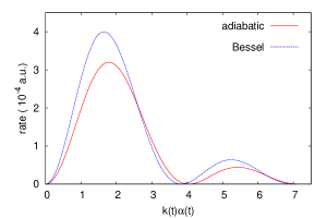
Figure 1: A solid line shows the single photon absorption rate as a function of $|k(t)|\alpha(t)$, given by Eq. (28b) for $n=1$. Here, $k(t)=\sqrt{2(E_{0}(t)+\omega)}$ is a momentum of an ionized electron, and $\alpha(t)$ the envelope function of our pulse defined in Eq. (6). A dot line shows an asymptotic result of Eq. (28b) for $\omega\to\infty$; see Eq. (29a). An oscillating feature of the rate comes from the Bessel function.

The second interference mechanism in Eq. (28a) is the temporal interference imprinted in $\cos$ function. The creation of the photo electron wave packet of the energy $E$ by the spatial interference takes place twice i.e. in the rising and falling part of the pulse, respectively. They interfere with the phase difference given by Eq. (28d), which represents the difference of the accumulation of the dynamical phase between them. The formula quite similar to Eq. (28) was found in the study of the oscillating substructure in photon absorption peaks in TT . The difference is that our formula does not take into account the depletion of the ground state since Eq. (28a) is obtained from the first order solution to Eq. (20); see Eqs. (21). However, the formula in TT was obtained in an empirical manner introducing a quasi static picture into the HFFT. In doing so, they obtained the single photon absorption rate as a function of time which exhibited clearly separated two peaks before and after the peak field amplitude of the pulse, which is the emergence of the stabilization i.e. the signature of the spatial interference in destructive way. This gave them the idea which two photo electron wave packets produced by the spatial interference in the rising and falling part of the pulse cause the temporal interference. However, as far as we know, it is first time to obtain the formula Eq. (28a) from the first principle which can capture the signatures of both the spatial and temporal interference in the spectrum. After the findings in TT , several groups had also found the temporal interference in high-frequency regime for hydrogen atom in DC , and also for hydrogen molecular ion YF ; YMad . However, in these studies, only the temporal interference was discussed since their pulse parameters are off the stabilization regime.

II.7 Numerical implementations

In this paper, we mainly study a photo detachment of hydrogen negative ion H^- in one dimension with single active electron approximation. The electron’s potential is modeled by PT

$$V(x)=-D\frac{\exp[-\sqrt{x^{2}+a^{2}}]}{\sqrt{x^{2}+b^{2}}},$$ (32a)

$$D=24.856,~{}~{}a=4,~{}~{}b=6.27.$$ (32b)

This potential supports only one bound state $E_{0}=-0.0277$. We employ the Siegert state expansion method in the KH frame, previously developed in TT to solve the full TDSE Eq. (1) and the envelope TDSE Eq. (13), and also Eq. (26).

III Results

III.1 Revisit of the oscillating substructure in photon absorption peaks

Fig. 2 shows a photo electron spectrum near a position of a photo peak $E=E_{0}(\pm\infty)+\omega$ for a set of laser parameters $F_{0}=0.5$, $\omega=\pi/10$ and $T=2000$. The solid line (red) and blank circles (red) represent the result of the full TDSE Eq. (1) and envelope TDSE Eq. (13), respectively. It is clearly shown that the envelope TDSE perfectly reproduces the full TDSE result. The overall structure is blue-shifted with respect to the photo peak at $E=E_{0}(\pm\infty)+\omega$ since the ground state energy $E_{0}(t)$ becomes shallower during the action of the pulse. The dotted (blue) and broken (blue) lines represent the result of the adiabatic approximation Eq. (23a) for $n=1$ and saddle point method Eq. (28a). The amplitudes of them are quite overestimated compared to the full TDSE calculation because the depletion of the ground state is ignored in the adiabatic approximation; Eq. (23a) is the first order solution to Eq. (20). And the phase shift of the interference structure is found for these results with respect to the full TDSE result Eq. (1). This is also due to the ignore of the depletion in the adiabatic approximation; the photo electron amplitude produced in the falling part of the pulse is largely overestimated. So, the relative phase of it with respect to that produced in the rising part of the pulse deviates from the exact calculation. The divergence around $E\approx E_{0}(\pm\infty)+\omega=0.2864$ and $E\approx E_{0}(0)+\omega=0.2965$ in the saddle point method are seen because time derivative of the ground state energy vanishes; see Eq. (28a). The former comes from the rising and falling edge of the pulse where the Stark dressing to the ground state is very small, and the latter at the peak intensity of the pulse. Since the saddle points $t_{-}$ and $t_{+}$ coalesce at the peak intensity, the divergence around the high energy edge can be removed by the uniform approximation Berry . The procedure is given in Appendix C. We consider that the oscillating substructure can be understood very well with the adiabatic approximation and saddle point method. Therefore, we thus conclude that the oscillating structure in photon absorption peak in high-frequency regime is formed by the spatial and temporal interference of photo electron wave packets discussed in Sec. II.6.

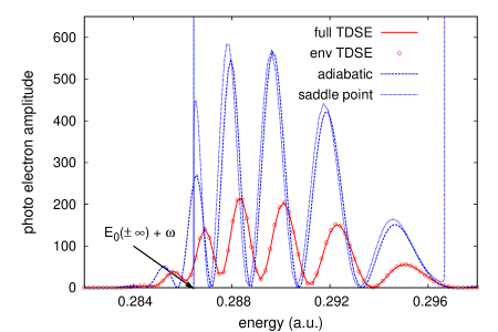
Figure 2: Photo electron spectrum for the laser parameters $F_{0}=0.5$, $\omega=\pi/10$, and $T=2000$ near a photo peak $E=E_{0}(\pm\infty)+\omega$ indicated by an arrow. The solid (green) and broken (red) lines are obtained by the envelope TDSE, Eq. (13) and the saddle point method Eq. (28a).

III.2 Time scale of non-adiabatic transition

In this subsection, we solve Eq. (26) for several model potentials to study the non-adiabatic transition. In the previous work TS , it was found that a yield of non-adiabatic transition has a maximum as a function of a pulse duration. One may consider that this is a mathematical artifact due to the normalization factor $\alpha_{0}$, Eq. (7), for our classical trajectory Eq. (5). For a limit of a pulse duration $T\to 0$, the yield vanishes because $\alpha_{0}$ becomes zero. And the yield also vanishes for a limit of $T\to\infty$ because the dressed potential $V_{0}(x,t)$ in Eq. (12a) varies infinitely slowly in time. Therefore, it is no wonder that a maximum can be found in between. However, a position of the maximum can be found in a region where the function $\alpha_{0}$ is almost converged to its asymptotic value $F_{0}/\omega^{2}$ for the limit $T\to\infty$, and the position is far away from a region where the function $\alpha_{0}$ rapidly converges to zero. Hence, the maximum has a physical origin rather than the mathematical artifact.

We consider small values of $\alpha_{0}$ to facilitate ourselves to derive formulas in perturbation theory to extract physics of the non-adiabatic transition. Up to the second order of $\alpha^{2}(t)$, a photo electron amplitude for the non-adiabatic transition $C^{(1)}_{0\omega}(k)$, Eq. (23a) for $n=0$, is reduced to,

$$C_{0\omega}^{(1)}(k) \approx D(k)f(E),$$ (33a)

$$D(k) = \langle k,t=-\infty|V^{\prime\prime}(x)|0(-\infty)\rangle,$$ (33b)

$$f(E) = -\frac{a}{T^{2}}\frac{1}{E-E_{0}(\pm\infty)}\int_{-\infty}^{\infty}t\alpha^{2}(t)e^{i\Phi_{0}(t)}dt.$$ (33c)

The function $\Phi_{0}(t)$ is given in Eq. (19). For simplicity, we ignore the Stark shift in the function $f(E)$. Then the function $f(E)$ is reduced to

$$f(E)\approx-i\sqrt{\frac{\pi}{32a}}\alpha_{0}^{2}Te^{-\frac{T^{2}}{8a}(E-E_{0}^{(0)})^{2}}.$$ (34a)

Therefore, we obtain the approximated spectrum of the non-adiabatic transition,

$$|C_{0\omega}^{(1)}(k)|^{2}=\frac{\pi}{32a}|D(k)|^{2}\alpha_{0}^{4}T^{2}e^{-\frac{T^{2}}{4a}(E-E_{0})^{2}},$$ (35)

Next, we derive the formula for the detachment yield. To implement this, we consider an ansatz for the functional form of $|D(k)|^{2}$,

$$|D(k)|^{2}=c_{1}k^{2}e^{-c_{2}\frac{k^{2}}{4aI_{p}}}.$$ (36a)

where $I_{p}=|E_{0}(\pm\infty)|$. The detachment probability $P_{0}(T)$ as a function of a pulse duration $T$ is calculated substituting Eq. (36a) into (35), and integrating over $k$,

$$P_{0}(T) = \int_{-\infty}^{\infty}|C_{0\omega}^{(0)}(k)|^{2}\frac{dk}{2\pi}$$ (37a)

$$= \frac{c_{1}}{2^{\frac{15}{4}}a^{\frac{1}{4}}}\alpha_{0}^{4}\sqrt{T}\xi^{\frac{3}{2}}e^{\xi^{2}-\frac{(I_{p}T)^{2}}{4a}}\left[K_{\frac{3}{4}}(\xi^{2})-K_{\frac{1}{4}}(\xi^{2})\right],$$

where the $$\xi$$ is defined as

$$\xi=\frac{1}{\sqrt{8a}}\frac{(I_{p}T)^{2}+c_{2}}{I_{p}T}.$$ (37b)

The derivation is found in Appendix A. In Appendix B, it is clarified that the constant $c_{2}$ is related to the curvature of the atomic potential.

Before calculating a position of a maximum of Eq. (37a), we take a limit of $\omega\to\infty$ for the formula. In doing so, the function $\alpha_{0}$ in Eq. (37a) sharply increases from 0, and quickly converges to its asymptotic value $F_{0}/\omega^{2}$ as $T$ increases. Then the maximum of Eq. (37a) takes place where the value of $\alpha_{0}$ is enough converged. It is thus guaranteed that the occurrence of the maximum of Eq. (37a) does not stem from our normalization factor $\alpha_{0}$, Eq. (7), for our normalized classical trajectory Eq. (5). Now we attempt to analytically extract an optimal pulse duration from Eq. (37a). We approximate the Bessel functions of fractional order $K_{\nu}(z)~{}(\nu=3/4~{}{\rm and}~{}1/4)$ in Eq. (37a) using its asymptotic form for large arguments,

$$K_{\nu}(z)\sim\sqrt{\frac{\pi}{2z}}e^{-z}\left[1+\frac{4\nu^{2}-1}{8z}\right].$$ (38)

This approximation becomes valid for $T\to 0$ and $T\to\infty$ since the argument $\xi$, Eq. (37b), diverges for these limit. The yield of the non-adiabatic ionization then becomes,

$$P_{0}\sim\frac{c_{1}\sqrt{\pi a}\alpha_{0}^{4}}{16\sqrt{I_{p}}}\frac{(I_{p}T)^{2}}{[(I_{p}T)^{2}+c_{2}]^{\frac{3}{2}}}e^{-\frac{(I_{p}T)^{2}}{4a}}.$$ (39)

The position of maximum is found solving $dP_{0}/d(I_{p}T)=0$. Then we obtain,

$$(I_{p}T)^{4}+(2a+c_{2})(I_{p}T)^{2}-4ac_{2}=0,$$ (40a)

The solution is

$$I_{p}T=\sqrt{\frac{1}{2}\left[-2a-c_{2}+\sqrt{4a^{2}+20ac_{2}+c_{2}^{2}}\right]}.$$ (40b)

We first demonstrate the result Eq. (40b) for a model potential of H^- Eq. (32). The parameters $c_{1}$ and $c_{2}$ for ansatz Eq. (36a) are found using fitting procedures, we obtain $c_{1}=1.76\times 10^{-3}$ and $c_{2}=0.301$. The result of the fitting is shown in Fig. 3(a). The solid (black) and dotted (blue) lines show the result obtained by Eqs. (33b) and (36a), respectively. We find that both the results agree very well. Next, we consider the high-frequency limit $\omega\to\infty$ to apply Eq. (40b). To this end, we introduce a scaling of $F_{0}$ and $\omega$ as

$$F_{0}\to m^{2}F_{0}~{}~{}~{}{\rm and}~{}~{}~{}\omega\to m\omega.$$ (41)

to keep a ratio $F_{0}/\omega^{2}$ being a constant, where $F_{0}=0.2$ and $\omega=\pi/10$. For the values of $m=1,2,4$ and $8$, we carried out solving Eq. (26). We terminated our calculations at $m=8$ since a peak position of the yield of the non-adiabatic transition it not significantly different comparing the result for $m=4$. This means that $T$ dependency in the function $\alpha_{0}$, Eq. (7) is washed out around a region where the peak position locates. Fig. 3(b) shows the detachment yield of the non-adiabatic transition. The solid (black) and broken (blue) line are obtained by the TDSE Eq. (26) and the asymptotic formula Eq. (39), respectively. The height of these lines are normalized to unity to clearly compare the peak positions. Substituting the value of the ionization potential $I_{p}=0.0277$ and $c_{2}=0.301$ to Eq. (40b), the expected optimal pulse duration is found to be $T_{\rm asym}=24.8$. This is about $20\%$ off the exact value $T=31$ shown in Fig. 3. We consider that this is reasonable in the rough approximations.

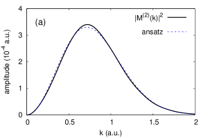
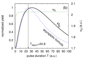
Figure 3: (a) Comparison between the numerically calculated matrix element $M^{(2)}(k)$, Eq. (33b), and its fitting by the ansatz Eq. (36a). (b) The solid line (black) shows the detachment yield by the non-adiabatic transitions for our model, Eq. (32), as a function of pulse duration obtained solving Eq. (26) with $\omega=4\pi/5$ and $F_{0}=12.8$. The broken line (blue) is obtained using the asymptotic formula Eq. (39) for $\omega\to\infty$ under the ansatz Eq. (36a). The maximum yields of these results are normalized to unity to clearly compare the positions of the peaks. The dot line shows the normalization factor $\alpha_{0}$ of our envelope function Eq. (7).

III.2.1 Effect of atomic structure on optimal pulse duration

We find that Eq. (40b) depends on the constant $c_{2}$, which is related to the curvature of the atomic potential $V(x)$. In harmonic approximation of the atomic potential, the curvature gives us a ground state energy; see Appendix B. To see effects of atomic structure on the optimal pulse duration, let us consider another atomic potential

$$W(x)=-W_{0}e^{-(x/\sigma)^{2}},$$ (42)

with different combinations of the parameters $W_{0}$ and $\sigma$ summarized in the table 1, which are referred as case I and II, respectively. The case I (II) represents a deep and narrow (shallow and wide) atomic potential. These combinations are chosen so that the field free ground state energy becomes $E_{0}(\pm\infty)=-0.1$. The values of $c_{1}$ and $c_{2}$ for the ansatz Eq. (36a) are summarized in Table 1. We repeated the scaling procedure Eq. (41) to reach high-frequency limit $\omega\to\infty$. In the case I (II), a peak position of a maximum yield of the non-adiabatic transition is converged for $m=32~{}(m=16)$. Substituting the parameter $c_{2}$ into Eq. (40b), which are given in table 1, we obtain

$${\rm case~{}I}~{}~{}~{}I_{p}T\approx 0.519~{}\rightarrow~{}T_{\rm asym} = 5.19,$$ (43a)

$${\rm case~{}II}~{}~{}~{}I_{p}T\approx 1.42~{}\rightarrow~{}T_{\rm asym} = 14.2.$$ (43b)

These values are also found in Table 1. Results are shown in Fig 4 and 5 for the case I and II, respectively, in a manner of Fig. 3. The quality of the asymptotic expansion of the modified Bessel function Eq. (38) near the origin for case II is better than the case I due to the bigger value of $c_{2}$; see Table 1. So, we obtain the better result for the position of the maximum yield in the case II than the case I.

It was shown in Fig. 4 of Tol that the yield of the non-adiabatic transition has a maximum for a certain value of a pulse duration, and it was estimated using $I_{p}T\approx 1$, which is equivalent to Eq. (40b) with the right hand side being unity. However, the right hand side of Eq. (40b) depends on not only binding energies but also curvatures of target potentials as shown in this demonstration.

	$W_{0}$	$\sigma$	$c_{1}$	$c_{2}$	$T_{\rm asym}$
case I	0.345	1	0.119	0.155	5.19
case II	0.159	4	0.00641	2.73	14.2

Table 1: Different combination of the parameters $W_{0}$ and $\sigma$ for the atomic potential Eq. (42) so that a field free ground state energy becomes $E_{0}(\pm\infty)=-0.1$. The parameters $c_{1}$ and $c_{2}$ are used for the ansatz Eq. (36a) to fit the matrix element $M^{(2)}(k)$, Eq. (33b). The value of $T_{\rm asym}$ is a predicted peak position of the detachment yield by the non-adiabatic transition Eq. (37a) using asymptotic formula Eq. (40b).

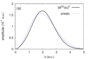
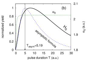
Figure 4: The same as Fig. 3 but another atomic potential Eq. (42) with the depth $W_{0}$ and the width $\sigma$ referred as case I in Table 1.

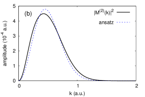
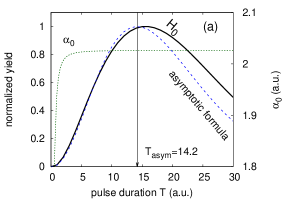
Figure 5: The same as Fig. 3 but another atomic potential Eq. (42) with the depth $W_{0}$ and the width $\sigma$ refereed as case II in Table 1.

IV conclusion

Following the previous work TS , we further explored a detachment dynamics of a model negative ion in high-frequency regime. We revisited the interference substructures in photon adsorption peaks in an adiabatic approximation based on the envelope Hamiltonian. The adiabatic approximation clarified that two different interference mechanisms are responsible for its emergence. The first mechanism is the spatial interference. At a certain time in a rising part of a pulse, two photo electron wave packets are launched at two turning points of a classical electron in the pulse. An interference of them create net amount of a photo electron wave packet. This spatial interference is repeated in the falling part of the pulse. Then these photo electron wave packets produced in different moments in time cause temporal interfere. We confirmed that the adiabatic approximation can well reproduce the oscillating substructure obtained from the full time-dependent Schrödinger equation (TDSE). The interference substructure was previously found in TT , and recently the same mechanism was confirmed for hydrogen atom in DC ; YMad . We showed that our theory is consistent with these known results. In TT , they predicted the coexistence of the spatial and temporal interference. However, their formulation was based on an empirical approach bringing a quasi static picture into the high-frequency Floquet theory GK . So, to our best knowledge, it is first time to find out both the interference mechanisms derived from the first principle.

We also extracted an optimal pulse duration to maximize a detachment yield by non-adiabatic transition. We clarified that the yield is maximized for a pulse duration close to time scale of non-adiabatic transition, roughly estimated by Eq. (40b).

Our demonstrations have been done utilizing short range potential, although our formulation does not depend on dimensionality and properties of atomic potential TS . Further studies in three-dimension in a real atomic system will be worked out in future.

V Acknowledgements

K. T. would thank for Profs. Ulf Saalmann and Jan M. Rost for the discussions to improve the manuscript.

Appendix A Derivation of Eq. (37a)

Substituting Eq. (36a) into (35), and integrating over $k$, the ionization yield of the non-adiabatic transition $P_{0}(T)$ is written as

$$P_{0}(T)=\int_{-\infty}^{\infty}|C_{0\omega}(k)|^{2}\frac{dk}{2\pi}=\frac{c_{1}\alpha_{0}^{4}\beta}{4}e^{-\frac{(I_{p}T)^{2}}{4a}}\int_{-\infty}^{\infty}k^{2}e^{-\beta k^{4}-\gamma k^{2}}dk,$$ (44a)

where

$$\beta = \frac{T^{2}}{16a},$$ (44b)

$$\gamma = \frac{I_{p}T^{2}}{4a}+\frac{c_{2}}{4aI_{p}}.$$ (44c)

The integral can be written using the fractional order $\nu$ of the modified Bessel function $I_{\nu}(z)$ of first kind,

$$\int_{-\infty}^{\infty}x^{2}e^{-\beta x^{4}-\gamma x^{2}}dx=\frac{\pi e^{\frac{\gamma^{2}}{8\beta}}}{8\sqrt{2}\beta^{\frac{3}{2}}\sqrt{\gamma}}\left[-\gamma^{2}I_{-\frac{1}{4}}\left(\frac{\gamma^{2}}{8\beta}\right)+(4\beta+\gamma^{2})I_{\frac{1}{4}}\left(\frac{\gamma^{2}}{8\beta}\right)\right.$$

$$\left.+\gamma^{2}\left\{-I_{\frac{3}{4}}\left(\frac{\gamma^{2}}{8\beta}\right)+I_{\frac{5}{4}}\left(\frac{\gamma^{2}}{8\beta}\right)\right\}\right].$$ (45a)

Using the properties of $$I_{\nu}(z)$$ nist ,

$$I_{\nu-1}(z)-I_{\nu+1}(z)=\frac{2\nu}{z}I_{\nu}(z),$$ (45b)

$$K_{\nu}(z)=\frac{\pi}{2}\frac{I_{-\nu}(z)-I_{\nu}(z)}{\sin(\nu\pi)},$$ (45c)

where $$K_{\nu}(z)$$ is the modified Bessel function of second kind, the integral can be simplified to

$$\int_{-\infty}^{\infty}x^{2}e^{-\beta x^{4}-\gamma x^{2}}dx=\frac{1}{8}\left(\frac{\gamma}{\beta}\right)^{\frac{3}{2}}e^{\frac{\gamma^{2}}{8\beta}}\left[K_{\frac{3}{4}}\left(\frac{\gamma^{2}}{8\beta}\right)-K_{\frac{1}{4}}\left(\frac{\gamma^{2}}{8\beta}\right)\right],$$ (45d)

Therefore, we obtain

$$P_{0}(T)=\frac{c_{1}}{2^{\frac{15}{4}}a^{\frac{1}{4}}}\alpha_{0}^{4}\sqrt{T}\xi^{\frac{3}{2}}e^{\xi^{2}-\frac{(I_{p}T)^{2}}{4a}}\left[K_{\frac{3}{4}}(\xi^{2})-K_{\frac{1}{4}}(\xi^{2})\right],$$ (46)

where

$$\xi=\frac{1}{\sqrt{8a}}\frac{(I_{p}T)^{2}+c_{2}}{I_{p}T}.$$ (47)

Appendix B Physical meaning of the constant $c_{2}$

The time-independent Schrödinger equation for the ground state $\phi_{0}$ with the energy $E_{0}$ reads,

$$\left[-\frac{1}{2}\frac{d^{2}}{dx^{2}}+V(x)\right]\phi_{0}(x)=E_{0}\phi_{0}(x),$$ (48)

Let us consider the Taylor expansion of the atomic potential $V(x)$ around the origin up to the order of $x^{2}$,

$$V(x)\approx V(0)+\frac{1}{2}\Omega^{2}x^{2},$$ (49)

where $\Omega^{2}=V^{\prime\prime}(0)$ represents the second derivative of atomic potential $V(x)$ at origin. In this approximation, the ground state $\phi_{0}^{(0)}(x)$ and its energy level $E_{0}^{(0)}$ thus correspond to those of simple harmonic oscillator, which are given by

$$\phi_{0}^{(0)}(x) = \left(\frac{\Omega}{\pi}\right)^{\frac{1}{4}}e^{-\frac{\Omega}{2}x^{2}},$$ (50a)

$$E_{0}^{(0)} = V(0)+\frac{\Omega}{2}.$$ (50b)

In what follows, we assume the condition of $E_{0}\approx E_{0}^{(0)}<0$. We exclude considering the case of $E_{0}^{(0)}>0$ which can happen for steep atomic potentials.

Now let us calculate the matrix element $M^{(2)}(k)$ Eq. (33b). To this end, we consider the case of $k\gg 1$. Then the scattering state can be replaced to $\langle k,t=\pm\infty|=e^{ikx}$. We approximate the ground state wave function $|0,t=\pm\infty\rangle$ by Eq. (50a). With these assumptions, substituting the expansion Eq. (49) into Eq. (33b),

$$|M^{(2)}(k)|^{2} = |\langle k,t=-\infty|V^{(2)}(x)|0,t=-\infty\rangle|^{2}$$ (51)

$$\approx \frac{\Omega^{\frac{9}{2}}}{\pi^{\frac{1}{2}}}\left|\int_{-\infty}^{\infty}e^{-\frac{1}{2}\Omega x^{2}}e^{ikx}dx\right|^{2}$$

$$= 2\sqrt{\pi}\Omega^{\frac{7}{2}}e^{-\frac{k^{2}}{\Omega}}.$$

This is the asymptotic formula of Eq. (36a) for $k\gg 1$. Therefore we obtain

$$\frac{c_{2}}{4aI_{p}}=\frac{1}{\Omega},~{}\rightarrow~{}c_{2}=\frac{4aI_{p}}{\Omega}.$$ (52)

For the 1D model of H^-, Eq. (32) and case I in Table 1 for the Gaussian potential Eq. (42), the ground state energy with harmonic approximation is bigger than $0$. So, the formulation in this appendix is not applicable. For the case II in table 1, $V^{(2)}(0)=0.02$ and $I_{p}=0.088$. On the other hand, the exact value is $I_{p}=0.1$. Then Eq. (52) gives us $c_{2}=3.45$, while the exact value shown in table 1 is $c_{2}=2.72$.

Appendix C Uniform approximation

The formulation here follows Berry Berry . To implement the uniform approximation, we introduce the mapping for Eq. (19)

$$\Phi_{n}(t)=-\int_{-\infty}^{t}E_{0}(t^{\prime})dt^{\prime}-n\omega t+Et=\zeta y+\frac{y^{3}}{3}+X.$$ (53)

Let $t=t_{\pm}$ satisfies the stationary phase condition,

$$\left(\frac{d\Phi}{dt}\right)_{t_{\pm}}=-E_{0}(t_{\pm})-\omega+E=(\zeta+y^{2})\left(\frac{dy}{dt}\right)_{t_{\pm}}=0,$$ (54)

then these are mapped onto

$$y_{\pm}=\pm i\sqrt{\zeta}.$$ (55)

Realising $y_{+}=-y_{-}$, the constant $X$ is given by

$$X=\frac{1}{2}\left[\Phi(t_{-})+\Phi(t_{+})\right].$$ (56)

Substituting Eqs. (55) and (56) into Eq. (53), we obtain,

$$\zeta=\left[-\frac{3i}{2}\theta(t_{+})\right]^{\frac{2}{3}}.$$ (57)

Another mapping we need is,

$$\frac{dt}{dy}M_{n\omega}(k,t)=p+qy.$$ (58)

Substituting $y=y_{\pm}$ into this equation, the constants $p$ and $q$ are determined as

$$p = \frac{1}{2}\left[\left(\frac{dt}{dy}\right)_{y_{+}}+\left(\frac{dt}{dy}\right)_{y_{-}}\right]M_{n\omega}(k,t_{+}),$$ (59a)

$$q = -\frac{i}{2\sqrt{\zeta}}\left[\left(\frac{dt}{dy}\right)_{y_{+}}-\left(\frac{dt}{dy}\right)_{y_{-}}\right]M_{n\omega}(k,t_{+})$$ (59b)

Note that the matrix element of the $n$photon absorption take the same value at $t=t_{\pm}$. To calculate the value of $dt/dy$, we twice differentiate Eq. (53) by $y$,

$$2y=\left[-E_{0}(t)-\omega+E\right]\frac{d^{2}t}{dy^{2}}-\frac{dE_{0}}{dt}\left(\frac{dt}{dy}\right)^{2}$$ (60)

Realising that $dt/dy$ is even function, substituting either $y=y_{-}$ or $y_{+}$, we obtain

$$\left(\frac{dt}{dy}\right)_{y_{\pm}}=\sqrt{\frac{-2i\zeta^{1/2}}{\dot{E_{0}}(t_{+})}},$$ (61a)

or

$$\left(\frac{dt}{dy}\right)_{y_{\pm}}=-\sqrt{\frac{-2i\zeta^{1/2}}{\dot{E_{0}}(t_{+})}}.$$ (61b)

Substituting this into Eq. (59), we thus obtain

$$p = \pm\sqrt{\frac{-2i\zeta^{1/2}}{\dot{E_{0}}(t_{+})}}M_{n\omega}(k,t_{+}),$$ (62a)

$$q = 0.$$ (62b)

The positive and negative sign of $p$ corresponds to the solution Eq. (61a) or (61b), respectively. Therefore, the photo electron amplitude for single photon absorption, Eq. (23a) for $n=1$, is given by

$$C_{n\omega}^{(1)}(k) = e^{iX}\int_{-\infty}^{\infty}\frac{dt}{dy}M_{n\omega}(k,t)e^{i(\zeta y+\frac{y^{3}}{3})}dy$$ (63)

$$= \pm 2\pi e^{iX}\sqrt{\frac{-2i\zeta^{1/2}}{E_{0}^{\prime}(t_{+})}}M_{n\omega}(k,t_{+}){\rm Ai}(\zeta)$$

$$= \pm e^{iX}\sqrt{\frac{-4\theta(t_{+})}{\dot{E_{0}}(t_{+})}}M_{n\omega}(k,t_{+})J_{\frac{1}{3}}\left(-\theta(t_{+})\right),$$

The function ${\rm Ai}(z)$ represents the Airy function. Here we used on the last line nist ,

$${\rm Ai}(z) = \frac{1}{\pi}\sqrt{\frac{z}{3}}K_{\frac{1}{3}}\left(\frac{2}{3}z^{\frac{3}{2}}\right),$$ (64a)

$$K_{\nu}(z) = J_{\nu}(iz)$$ (64b)

where the function $K_{\nu}(z)$ and $J_{\nu}(z)$ are the modified Bessel function of fractional order $\nu$, and Bessel function of fractional order $\nu$, respectively. Substituting the asymptotic form of the matrix element for the $n$photon absorption Eq. (29a) into Eq. (63),

$$C_{n\omega}^{(1)}(k) = \pm i^{n}e^{i(X-n\delta)}\sqrt{\frac{4\theta(t_{+})}{\dot{E_{0}}(t_{+})}}A(k(t_{+}))\varphi_{0}(-\alpha(t_{+}))$$ (65)

$$\times J_{n}(|k(t_{+})|\alpha(t_{+}))J_{\frac{1}{3}}\left(-\theta(t_{+})\right)$$

It is found that the spectrum is written using two Bessel functions. The Bessel function of the integer order $n$ represents the spatial interference, and the fractional order $1/3$ temporal interference. It is easily shown by L’Hôpital’s rule that the quantity $\theta(t_{+})/\dot{E_{0}}(t)$ is order of $t_{+}^{2}$ at the vicinity of $t_{+}=0$. Therefore, the result Eq. (65) does not have the singularity at $t_{+}=0$.

References

- (1) M. Chini, K. Ahao, and Z. Chang, Nat. Photonics 8, 437 (2014).
- (2) M. Gavrila and J. Z. Kaminski, Phys. Rev. Lett. 52, 613 (1984).
- (3) W. C. Henneberger, Phys. Rev. Lett. 21, 838 (1968).
- (4) M. Pont and M. Gavrila, Phys. Rev. Lett. 65, 2362 (1990).
- (5) L. You, J. Mostowski, and J. Cooper, Phys. Rev. A 45, 3203 (1992).
- (6) K. Toyota, U. Saalmann, and J. M. Rost, New J. Phys. 17, 073005 (2015).
- (7) K. Toyota, O. I. Tolstikhin, T. Morishita, and S. Watanabe, Phys. Rev. A 76, 043418 (2007).
- (8) P. V. Demekhin and L. S. Cederbaum, Phys. Rev. Lett. 108, 253001 (2012).
- (9) R. R. Jones, Phys. Rev. Lett. 74, 1091 (1995).
- (10) V. C. Reed and K. Burnett, Phys. Rev. A 43, 6217 (1991).
- (11) C. Yu, N. Fu, T. Hu, G. Zhang, and J. Yao, Phys. Rev. A 88, 043408 (2013).
- (12) L. Yue, and, L. B. Madsen, Phys. Rev. A 90, 063408 (2014).
- (13) K. Toyota, O. I. Tolstikhin, T. Morishita, and S. Watanabe, Phys. Rev. Lett. 103, 153003 (2009).
- (14) O. I. Tolstikhin, Phys. Rev. A 77, 032711 (2008).
- (15) M. Tilly, A. Karamatskou, and R. Santra, J. Phys. B 48, 124001 (2015).
- (16) D. Barash, A. E. Orel, and R. Baer, Phys. Rev. A 61, 013402 (1999).
- (17) M. Førre, S. Selstø, J. P. Hansen, and L. B. Madsen, Phys. Rev. Lett 95, 043601 (2005).
- (18) A. M. Popov, O. V.Tikhonova, and E. A. Volkova, J. Phys. B: At. Mol. Phys. 32 (1999).
- (19) M. Pont, Phys. Rev. A 44, 2141 (1991).
- (20) G. Yao and Shih-I. Chu, Phys. Rev. A 45, 6735 (1992).
- (21) M. V. Berry, Proc. Phys. Soc. 89, 479 (1966).
- (22) F. W. J. Olver, D. W. Lozier, R. F. Boisvert, and C. W. Clark, NIST Handbook of Mathematical Functions (Cambridge University Press, New York, 2010)