Restarting for the Tensor Infinite Arnoldi method

Abstract

An efficient and robust restart strategy is important for any Krylov–based method for eigenvalue problems. The tensor infinite Arnoldi method (TIAR) is a Krylov–based method for solving nonlinear eigenvalue problems (NEPs). This method can be interpreted as an Arnoldi method applied to a linear and infinite dimensional eigenvalue problem where the Krylov basis consists of polynomials. We propose new restart techniques for TIAR and analyze efficiency and robustness. More precisely, we consider an extension of TIAR which corresponds to generating the Krylov space using not only polynomials but also structured functions that are sums of exponentials and polynomials, while maintaining a memory efficient tensor representation. We propose two restarting strategies, both derived from the specific structure of the infinite dimensional Arnoldi factorization. One restarting strategy, which we call semi–explicit TIAR restart, provides the possibility to carry out locking in a compact way. The other strategy, which we call implicit TIAR restart, is based on the Krylov–Schur restart method for linear eigenvalue problem and preserves its robustness. Both restarting strategies involve approximations of the tensor structured factorization in order to reduce complexity and required memory resources. We bound the error in the infinite dimensional Arnoldi factorization showing that the approximation does not substantially influence the robustness of the restart approach. We illustrate the approaches by applying them to solve large scale NEPs that arise from a delay differential equation and a wave propagation problem. The advantages in comparison to other restart methods are also illustrated.

1 Introduction

We consider the nonlinear eigenvalue problem (NEP) defined as finding $(\lambda,v)\in\mathbb{C}\times\mathbb{C}^{n}\setminus\left\{0\right\}$ such that

$$M(\lambda)v=0$$ (1)

where $\lambda\in\Omega\subseteq\mathbb{C}$, $\Omega$ is an open disk centered in the origin and $M:\Omega\rightarrow\mathbb{C}^{n\times n}$ is analytic. The NEP has received a considerable attention in literature. See the review papers Mehrmann2004nonlinear ; Voss_2013_NEPCHAPTER and the problem collection NLEP_COLLECTION_2011 .

There are specialized methods for solving different classes of NEPs such as polynomial eigenvalue problems (PEPs) see mackey2015_PEP ; mehrmann2006structured_PEP ; lancaster2005pseudospectra and (bai2000templates, , Chapter 9), in particular quadratic eigenvalue problems (QEPs) tisseur2001quadratic ; meerbergen2008quadratic ; meerbergen2001locking ; bai2005soar and rational eigenvalue problems (REPs) voss2003maxmin ; betcke2008restarting ; betcke2016restarting ; su2011rep . There are also methods that exploit the structure of the operator $M(\lambda)$ like Hermitian structure szyld2015Hermitian_part1 ; szyld2015Hermitian_part2 or low rank of the matrix–coefficients van2016rank . Methods for solving a more general class of NEP are also present in literature. There exist methods based on modification of the Arnoldi method voss2004arnoldi , which can be restarted for certain problems, Jacobi–Davidson methods betcke2004jacobi_davidson , Newton–like methods kressner2009blockNewton ; neumaier1985residual ; effenberger2013robust and Arnoldi–like methods combined with a companion linearization of $M(\lambda)$ guttel2014nleigs ; Beeumen_CORK_2015 ; Jarlebring_INFARN_2012 .

We do not assume any particular structure of the NEP except for the analyticity and the computability of certain quantities associated with $M(\lambda)$ (further described later). In this paper we consider the Infinite Arnoldi method (IAR) Jarlebring_INFARN_2012 , which is equivalent to the Arnoldi method applied to a linear operator. More precisely, under the assumption that zero is not an eigenvalue, the problem (1) can be reformulated as $\lambda B(\lambda)v=v$, where $B(\lambda)=M(0)^{-1}(M(0)-M(\lambda))/\lambda$. This problem is equivalent to the linear and infinite dimensional eigenvalue problem $\lambda\mathcal{B}\psi(\theta)=\psi(\theta)$, where $\psi(\theta):\mathbb{C}\rightarrow\mathbb{C}$ is an analytic function (Jarlebring_INFARN_2012, , Theorem 3). The operator $\mathcal{B}$ is linear, maps functions to functions, and is defined as

$$\mathcal{B}\psi(\theta):=\int_{0}^{\theta}\psi(\hat{\theta})d\hat{\theta}+C(\psi),$$

where

$$C(\psi):=\sum_{i=0}^{\infty}\frac{B^{(i)}(0)}{i!}\psi^{(i)}(0).$$

The Tensor Infinite Arnoldi (TIAR), which is an improvement of IAR, was presented in WAVEGUIDE_ARNOLDI_2015 . This method is equivalent to IAR but computationally more attractive. In contrast to IAR, the basis of the Krylov space, which consists of polynomials, is implicitly represented in a memory efficient way. This improves the performances in terms of memory and CPU-time. Another improvement of IAR was presented in Jarlebring2014Schur . This method consists in generating the Krylov space by using structured functions, which are sums of polynomials and exponential functions. The main advantage of this approach is the possibility to perform a semi–explicit restart by imposing the structure. In this paper extend the framework of TIAR to structured functions and study restart techniques.

A problematic aspect of any algorithm based on the Arnoldi method is that, when many iterations are performed, there are numerical complexity and stability issues. Fortunately, an appropriate restart of the algorithm can partially resolve these issues. There exist two main classes of restarting strategies: explicit restart and implicit restart. Most of the explicit restart techniques consist in selecting a starting vector that generates an Arnoldi factorization with the wanted Ritz values. The implicit restart consists computing a new Arnoldi factorization with the wanted Ritz values. This process can be done deflating the unwanted Ritz values as in, e.g., IRA Sorensen_IRA_1996 or extracting a proper subspace of the Krylov space by using the Krylov–Schur restart approach Stewart2002KrylovSchur . Both approaches are mathematically equivalent. For reasons of numerical stability it is in general preferable to use implicit restart. See Morgan96RestartArnoldi for further discussions about the restart of the Arnoldi method for the linear eigenvalue problems.

The paper is organized as follows: in Section 2 we extend TIAR to tensor structured function. In Section 4 we propose a semi–explicit restart for TIAR. This new algorithm is equivalent to Jarlebring2014Schur but the implicit representation of the Krylov basis gives an improvements in terms of memory and CPU time. In section 5 we propose an implicit restart for TIAR based on an adaption of Krylov–Schur restart. The Krylov–Schur restart for the Arnoldi method in the linear case has constant CPU–time for outer iteration. In contrast to this, a direct usage of the Krylov–Schur restart for TIAR does not give a substantial improvement due to the memory efficient representation of the Krylov basis. We show that the structure of the Arnoldi factorization allow us to perform approximations that reduce the complexity and the memory requirements. We prove that the coefficients matrix representing the basis of the Kylov space present a fast decay in the singular values. Therefore we use this in a derivation of a low rank approximation of such matrices. Moreover we prove that there is a fast decay in the coefficients of the polynomial part of the functions in the Krylov space. This can be used to introduce another approximation when the power series coefficients of $M(\lambda)$ decay to zero . We give explicit bounds on the errors due to those approximations.

There exist other Arnoldi–like methods combined with a companion linearization that use memory efficient representation of the Krylov basis matrix. See CORK Beeumen_CORK_2015 , TOAR Kressner_and_Roman_compact_2014 and zhang2013memory . Similar to TIAR, the direct usage of the Krylov–Schur restart for these methods does not decrease the complexity unless svd–based approximations are used. More precisely, the coefficients that represent the Krylov basis are replaced with their low rank approximations. In contrast to those approaches, our specific setting allow us to characterize the impact of the approximations.

Finally, in Section 7 we show, with numerical simulations, the effectiveness of the restarting strategies.

2 Tensor structured functions and TIAR factorizations

Similar to many restart strategies for linear eigenvalue problems, our approach is based on computation, representation and manipulation of an Arnoldi-type factorization. For our infinite-dimensional operator, the analogous Arnoldi-type factorization is defined as follows. The functions $\Psi_{k}$ are represented with a particular tensor structure which we further described in Section 2.1.

Definition 2.1 (TIAR factorization)

Let $\Psi_{k+1}(\theta)$ be a tensor structured
function with orthogonal columns and let $\underline{H}_{k}\in\mathbb{C}^{(k+1)\times k}$ be an Hessenberg matrix with positive elements in the sub–diagonal. The pair $(\Psi_{k+1},\underline{H}_{k})$ is a TIAR factorization of length $k$ if

$$\mathcal{B}\Psi_{k}(\theta)=\Psi_{k+1}(\theta)\underline{H}_{k}.$$ (2)

2.1 Representation and properties of the tensor structred functions

We consider a class of structured functions introduced in Jarlebring2014Schur , represented in a different and memory–efficient way.

Definition 2.2

The vector–valued function $\psi:\mathbb{C}\rightarrow\mathbb{C}^{n}$ is a tensor structured function if it exist $Y,W\in\mathbb{C}^{n\times p}$, $\bar{a}\in\mathbb{C}^{d\times r}$, $\bar{b}\in\mathbb{C}^{d\times p}$, $\bar{c}\in\mathbb{C}^{p}$, $S\in\mathbb{C}^{p\times p}$, $Z\in\mathbb{C}^{n\times r}$ where $[Z,\ W]$ is orthogonal and $\operatorname{span}(Y)=\operatorname{span}(W)$, such that

$$\psi(\theta)= P_{d-1}(\theta)\left(\sum_{\ell=1}^{r}\bar{a}_{:,\ell}\otimes z_{\ell}+\sum_{\ell=1}^{p}\bar{b}_{:,\ell}\otimes w_{\ell}\right)+Y\exp_{d-1}(\theta S)\bar{c}$$ (3)

where

$$P_{d}(\theta):=(1,\theta,\dots,\theta^{d})\otimes I_{n}$$ (4)

and $\exp_{d-1}(\theta S):=\sum_{i=d}^{\infty}\theta^{i}S^{i}$ is consistent with Jarlebring2014Schur .

The matrix–valued functions $\Psi_{k}:\mathbb{C}\rightarrow\mathbb{C}^{n\times k}$ is a tensor structured function if it can be expressed as $\Psi_{k}(\theta)=(\psi_{1}(\theta),\dots,\psi_{k}(\theta))$, where each $\psi_{i}$ is a tensor structured function. We denote the $i$–th column of $\Psi_{k}$ by $\psi_{i}$. The structure induced by (3) is now, in a compact form

$$\Psi_{k}(\theta)= P_{d-1}(\theta)\left(\sum_{\ell=1}^{r}a_{:,:,\ell}\otimes z_{\ell}+\sum_{\ell=1}^{p}b_{:,:,\ell}\otimes w_{\ell}\right)+Y\exp_{d-1}(\theta S)C$$ (5)

where $a\in\mathbb{C}^{d\times k\times r}$, $b\in\mathbb{C}^{d\times k\times p}$, $C\in\mathbb{C}^{p\times k}$. We say that $\Psi_{k}(\theta)$ is orthogonal if the columns are orthogonormal, i.e., $<\psi_{i}(\theta),\psi_{j}(\theta)>=\delta_{i,j}$ for $i,j=1,\dots,k$. We use the scalar product consistent with the other papers about the infinite Arnoldi method Jarlebring2014Schur ; Jarlebring_INFARN_2012 , i.e., if $\psi(\theta)=\sum_{i=0}^{\infty}\theta^{i}x_{i}$ and $\varphi(\theta)=\sum_{i=0}^{\infty}\theta^{i}y_{i}$, then

$$<\psi,\varphi>=\sum_{i=0}^{\infty}<x_{i},y_{i}>.$$

The computation of this scalar product and norms for the tensor structured functions (3) can be done analogous to Jarlebring2014Schur . In particular, by definition of (4) we have

$$\|P_{d-1}(\theta)W\|=\|W\|_{F}$$ (6)

for any $W\in\mathbb{C}^{nd\times p}$.

Remark 2.3 (Representation of tensor structured functions)

The polynomial part of a tensor structured function (5) is a linear combination of the columns of the matrices $Z$ and $W$ using the coefficients given by the tensors $a$ and $b$. The exponential part is given by a linear combination of the columns of the matrix $Y$ and using as coefficients the matrix $C$ multiplied by the powers of $S$. Therefore we can represent a tensor structured function (5) using the matrices $(Z,W,Y,S)$ and the coefficients $(a,b,C)$.

Observation 2.4 (Linearity with respect the coefficients)

Given the tensor structured function $\Psi_{k}(\theta)$ represented by $(Z,W,Y,S)$ with coefficients $(a,b,C)$ and $\tilde{\Psi}_{\tilde{k}}(\theta)$ represented by the same matrices but with coefficients $(\tilde{a},\tilde{b},\tilde{C})$. The function $\hat{\Psi}_{\hat{k}}(\theta)=\Psi_{k}(\theta)M+\tilde{\Psi}_{\tilde{k}}(\theta)N$ is also a tensor structured function represented by the same matrices and coefficients $(\hat{a},\hat{b},\hat{C})$ where for $\ell=1,\dots,r$ we have defined

$$\hat{a}_{:,:,\ell}:=a_{:,:,\ell}M+\tilde{a}_{:,:,\ell}N \hat{b}_{:,:,\ell}:=b_{:,:,\ell}M+\tilde{b}_{:,:,\ell}N \hat{C}:=CM+\tilde{C}N$$

We use the following notation $M_{i}:=M^{(i)}(0)$ and $\mathbb{M}_{d}(Y,S)$ is defined as in Jarlebring2014Schur . In particular, any nonlinear function $M$ can be represented as a sum of products of scalar nonlinearities

$$M(\lambda)=\sum_{i=1}^{q}T_{i}f_{i}(\lambda),\;\;\;\;T_{i}\in\mathbb{C}^{n\times n},f_{i}:\Omega\rightarrow\mathbb{C},\;i=1,\ldots,q,$$ (7)

and we define $\mathbb{M}_{d}:\mathbb{C}^{n\times p}\times\mathbb{C}^{p\times p}\rightarrow\mathbb{C}^{n\times p}$ as

$$\mathbb{M}_{d}(Y,S):=\sum_{i=1}^{q}F_{i}Yf_{i}(S)-\sum_{i=1}^{d}\frac{M_{i}YS^{i}}{i!},$$ (8)

which equivalently can be expressed as

$$\mathbb{M}_{d}(Y,S)=\sum_{i=d+1}^{\infty}\frac{M_{i}YS^{i}}{i!}.$$ (9)

The action of the operator $\mathcal{B}$ on functions represented as in (3) can now be expressed in a closed form using the notation above.

Theorem 2.5 (Action of $\mathcal{B}$)

Suppose $Y,W\in\mathbb{C}^{n\times p}$, $Z\in\mathbb{C}^{n\times r}$, $\bar{a}\in\mathbb{C}^{d\times r}$, $\bar{b}\in\mathbb{C}^{d\times p}$, $\bar{c}\in\mathbb{C}^{p}$ and $S\in\mathbb{C}^{p\times p}$. Suppose $\lambda(S)\subset\Omega$, let $\tilde{c}=S^{-1}\bar{c}$ and

$$\tilde{z}:=-M_{0}^{-1}\left[\mathbb{M}_{d}(Y,S)\tilde{c}-\sum_{i=1}^{d}M_{i}\left(\sum_{i=1}^{r}\frac{\bar{a}_{i,\ell}}{i}z_{\ell}+\sum_{\ell=1}^{p}\frac{\bar{b}_{i,\ell}}{i}w_{\ell}\right)\right].$$ (10)

Under the assumption that

$$\tilde{z}\not\in\operatorname{span}(z_{1},\dots,z_{r},w_{1},\dots,w_{p}),$$ (11)

let $z_{r+1}$ be the normalized orthogonal complement of $\tilde{z}$ against $z_{1},\dots,z_{r}$, $w_{1},\dots,w_{p}$ and $\tilde{a}_{1,\ell}$ and $\tilde{b}_{1,\ell}$ be the orthonormalization coefficients, i.e.,

$$\tilde{z}=\sum_{i=1}^{r+1}\tilde{a}_{1,\ell}z_{i}+\sum_{i=1}^{p}\tilde{b}_{1,\ell}w_{i}.$$ (12)

Then, the action of $\mathcal{B}$ on the tensor structured function defined by (3) is

$$\mathcal{B}\psi(\theta)=P_{d}(\theta)\left(\sum_{\ell=1}^{r+1}\tilde{a}_{:,\ell}\otimes z_{\ell}+\sum_{\ell=1}^{p}\tilde{b}_{i,\ell}\otimes w_{\ell}\right)+Y\exp_{d}(\theta S)\tilde{c}$$ (13)

where

$$\tilde{a}_{i,r+1}:=0, i=1,\dots,d\$$ (14a)

$$\tilde{a}_{i+1,\ell}:=\bar{a}_{i,\ell}/i, i=1,\dots,d\ ;\ \ell=1,\dots,r$$ (14b)

$$\tilde{b}_{i+1,\ell}:=\bar{b}_{i,\ell}/i, i=1,\dots,d\ ;\ \ell=1,\dots,p.$$ (14c)

Proof

With the notation

$$x_{i}:=\sum_{\ell=1}^{r}\bar{a}_{i+1,\ell}z_{\ell}+\sum_{\ell=1}^{p}\bar{b}_{i+1,\ell}w_{\ell} i=0,\dots,d-1$$ (15)

and $x:={\operatorname{vec}}(x_{0},\dots,x_{d-1})\in\mathbb{C}^{dn}$, $\psi(\theta)$ defined in (3) can be expressed as

$$\psi(\theta)=P_{d-1}(\theta)x+Y\exp_{d-1}(\theta S)\bar{c}$$ (16)

By invoking (Jarlebring2014Schur, , theorem 4.2) and using (15), we can express the action of the operator as

$$\mathcal{B}\psi(\theta)=P_{d}(\theta)x_{+}+Y\exp_{d}(\theta S)\tilde{c}$$ (17)

where $x_{+}:={\operatorname{vec}}(x_{+,0},\dots,x_{+,d})\in\mathbb{C}^{(d+1)n}$ with

$$x_{+,i} :=\sum_{i=1}^{r}\frac{\bar{a}_{i,\ell}}{i}z_{\ell}+\sum_{\ell=1}^{p}\frac{\bar{b}_{i,\ell}}{i}w_{\ell} i=1,\dots,d$$ (18)

$$x_{+,0} :=-M_{0}^{-1}\left(\mathbb{M}_{d}(Y,S)\tilde{c}+\sum_{i=1}^{d}M_{i}x_{+,i}\right).$$ (19)

Substituting (18) in (19) we obtain $x_{+,0}=\tilde{z}$ given in (10). Using (14) and (12) we can express $x_{+}$ in terms of $\tilde{a}$ and $\tilde{b}$ and we conclude by substituting this expression for $x_{+}$ in (17).

Remark 2.6

The assumption (11) can only be satisfied if $r+p\leq n$. This is the case that we are considering in this paper, since we assume the NEP to be large–scale and in Section 5.1 we introduce approximations that avoid $r$ from being large. The hypothesis $\lambda(S)\subseteq\Omega$ is necessary in order to define $\mathbb{M}_{d}(Y,S)$ that is used to compute $\tilde{z}$ in equation (10).

2.2 Orthogonalization

In order to expand a TIAR factorization $(\Psi_{k},\underline{H}_{k-1})$, we need to orthogonalize the tensor structured function $\mathcal{B}\psi_{k}$ (computed using the theorem 2.5) against the columns of $\Psi_{k}(\theta)$. The degree of $\Psi_{k}(\theta)$ is $d-1$ whereas the degree of $\mathcal{B}\psi_{k}(\theta)$ is $d$. In order to perform the orthogonalization, we transform them to the same degree $d$. Starting from (5) we can rewrite $\Psi_{k}$ as

$$\Psi_{k}(\theta)=P_{d-1}(\theta)\left(\sum_{\ell=1}^{r}a_{:,:,\ell}\otimes z_{\ell}+\sum_{\ell=1}^{p}b_{:,:,\ell}\otimes w_{\ell}\right)+\frac{YS^{d}C}{d!}\theta^{d}+Y\exp_{d}(\theta S)C.$$ (20)

We define

$$\begin{array}[]{ccc}\displaystyle E:=\frac{W^{H}YS^{d}C}{d!}&&\begin{array}[]{clcl}a_{d,j,\ell}&:=0&&\ell=1,\dots,r+1\\ b_{d,j,\ell}&:=e_{\ell,j}&&\ell=1,\dots,p\end{array}\end{array}$$ (21)

for $j=1,\dots,k$. Since $\operatorname{span}(W)=\operatorname{span}(Y)$ and, since $W$ is orthogonal, we have that $Y=WW^{H}Y$. Hence, using this relation and (21), the function $\Psi_{k}$ in (20) can be expressed as

$$\Psi_{k}(\theta)=P_{d}(\theta)\left(\sum_{\ell=1}^{r}a_{:,:,\ell}\otimes z_{\ell}+\sum_{\ell=1}^{p}b_{:,:,\ell}\otimes w_{\ell}\right)+Y\exp_{d}(\theta S)C$$

Theorem 2.7 (Orthogonalization)

Let $(Z,W,Y,S)\in\mathbb{C}^{n\times r}\times\mathbb{C}^{n\times p}\times\mathbb{C}^{n\times p}\times\mathbb{C}^{p\times p}$ be the matrices and $(a,b,C),(\bar{a},\bar{b},\bar{c})\in\mathbb{C}^{d\times\bar{k}\times r}\times\mathbb{C}^{d\times\bar{k}\times p}\times\mathbb{C}^{p\times\bar{k}}$ the coefficients that represent $\psi(\theta)$ given in (3) and $\Psi_{k}(\theta)$ given in (5). Let

$$h=\sum_{\ell=1}^{r}(a_{:,:,\ell})^{H}\bar{a}_{:,\ell}+\sum_{\ell=1}^{p}(b_{:,:,\ell})^{H}\bar{b}_{:,\ell}+\sum_{i=d}^{\infty}C^{H}\frac{(S^{i})^{H}Y^{H}YS^{i}}{(i!)^{2}}\bar{c}$$ (22)

The orthogonal complement of $\psi(\theta)$ against the columns of $\Psi_{k}(\theta)$ is

$$\psi^{\perp}(\theta)=P_{d-1}(\theta)\left(\sum_{\ell=1}^{r}a_{:,\ell}^{\perp}\otimes z_{\ell}+\sum_{\ell=1}^{p}b_{:,\ell}^{\perp}\otimes w_{\ell}\right)+Y\exp_{d-1}(\theta S)c^{\perp}$$

where

$$c^{\perp} =\bar{c}-Ch$$ (23a)

$$a_{:,\ell}^{\perp} =\bar{a}_{:,\ell}-a_{:,:,\ell}h \ell=1,\dots,r$$ (23b)

$$b_{:,\ell}^{\perp} =\bar{b}_{:,\ell}-b_{:,:,\ell}h \ell=1,\dots,p$$ (23c)

The vector $h$ contains the orthogonalization coefficients, i.e., $h_{j}=<\psi_{i},\psi>$. Moreover, given

$$\beta:=\sqrt{\|b^{\perp}\|_{F}^{2}+\|a^{\perp}\|_{F}^{2}+\sum_{i=d}^{\infty}\frac{\left(c^{\perp}\right)^{H}\left(S^{i}\right)^{H}Y^{H}YS^{i}c^{\perp}}{(i!)^{2}}}$$ (24)

it holds $\|\psi^{\perp}\|=\beta$.

Proof

Let us define $h_{j}:=<\psi_{j},\psi>$ for $j=1,\dots,k$, we have that the orthogonal complement, computed with the Gram–Schmidt process, is $\psi^{\perp}(\theta)=\psi(\theta)-\Psi_{k}(\theta)h$. Using the Observation 2.4 we obtain directly (23).

We express $\psi(\theta)$ as (16) and, the columns of $\Psi_{k}$ as

$$\psi_{j}(\theta)=P_{d-1}(\theta)x^{(j)}+Y\exp_{d-1}(\theta S)c_{j}$$ (25)

where $x^{(j)}:={\operatorname{vec}}(x_{0}^{(j)},\dots,x_{d-1}^{(j)})\in\mathbb{C}^{dn}$, with

$$x_{i}^{(j)}:=\sum_{i=1}^{r}\bar{a}_{i+1,j,\ell}z_{\ell}+\sum_{\ell=1}^{p}\bar{b}_{i+1,j,\ell}w_{\ell} i=0,\dots,d-1.$$ (26)

By applying (Jarlebring2014Schur, , equation (4.32)) we obtain

$$h_{j}=\sum_{i=0}^{d-1}(x_{i}^{(j)})^{H}x_{i}+c_{j}^{H}\sum_{i=d}^{\infty}\frac{(S^{i})^{H}Y^{H}YS^{i}}{(i!)^{2}}\bar{c} j=1,\dots,k.$$ (27)

We now substitute (15) and (26) in (27) and use the orthogonormality of the vectors $z_{1},\dots,z_{r}$, $w_{1},\dots,w_{p}$ and we find that

$$h_{j}=\sum_{\ell=1}^{r}(a_{:,j,\ell})^{H}\bar{a}_{:,\ell}+\sum_{\ell=1}^{p}(b_{:,j,\ell})^{H}\bar{b}_{:,\ell}+\sum_{i=d}^{\infty}c_{j}^{H}\frac{(S^{i})^{H}Y^{H}YS^{i}}{(i!)^{2}}\bar{c} j=1,\dots,k.$$

Which are the elements of the right–hand side of obtain (22). Using that $\|\psi^{\perp}\|^{2}=<\psi^{\perp},\psi^{\perp}>$ and repeating the same reasoning we have

$$\|\psi^{\perp}\|^{2} =\sum_{\ell=1}^{r}(a^{\perp}_{:,\ell})^{H}a^{\perp}_{:,\ell}+\sum_{\ell=1}^{p}(b^{\perp}_{:,\ell})^{H}b^{\perp}_{:,\ell}+\sum_{i=d}^{\infty}\frac{\left(c^{\perp}\right)^{H}\left(S^{i}\right)^{H}Y^{H}YS^{i}c^{\perp}}{(i!)^{2}}.$$

which proves (24).

2.3 A TIAR expansion algorithm in finite dimension

One algorithmic component common in many restart procedures is the expansion of an Arnoldi-type factorizations. The standard way to expand Arnoldi-type factorizations (as, e.g., described in (Stewart2002KrylovSchur, , Section 3)) involves the computation of the action of the operator/matrix and orthogonalization. We now show how we can carry out an expansion of the infinite dimensional TIAR-factorization (2) by only using operations on matrices and vectors of finite dimension.

In the previous subsections we presented the action of the operator $\mathcal{B}$ and orthogonalization for tensor structured functions (3). These results can be directly combined to expand the TIAR factorization. The resulting algorithm is summarized in Algorithm 1. The action of the operator $\mathcal{B}$ described in Theorem 2.5 is expressed in Steps 1-1. The orthogonalization of the new function using Theorem 2.7 is expressed in Steps 1-7 and Step 1 corresponds to increasing the degree as described in (20) and (21). Due to the representation of $\Psi_{k}$ as tensor structured function, the expansion with one column corresponds to an expansion of all the coefficients representing $\Psi_{k}$. This expansion is visualized in Figure 1.

input :  A TIAR factorization $(\Psi_{\bar{k}+1},\underline{H}_{\bar{k}})$ represented by $(Z,W,Y,S)\in\mathbb{C}^{n\times r}\times\mathbb{C}^{n\times p}\times\mathbb{C}^{n\times p}\times\mathbb{C}^{p\times p}$ and $(a,b,C)\in\mathbb{C}^{d\times\bar{k}\times r}\times\mathbb{C}^{d\times\bar{k}\times p}\times\mathbb{C}^{p\times\bar{k}}$.

output :  A TIAR factorization $(\Psi_{m+1},\underline{H}_{m})$ represented by $(Z,W,Y,S)\in\mathbb{C}^{n\times\tilde{r}}\times\mathbb{C}^{n\times p}\times\mathbb{C}^{n\times p}\times\mathbb{C}^{p\times p}$ and $(a,b,C)\in\mathbb{C}^{\tilde{d}\times m\times r}\times\mathbb{C}^{\tilde{d}\times m\times p}\times\mathbb{C}^{p\times m}$ where $\tilde{r}=r+m-\bar{k}$ and $\tilde{d}=d+m-\bar{k}$.

1 Set $\tilde{r}=r$, $\tilde{d}=d$

for $k=\bar{k}+1,2,\ldots,m$  do

      2 Compute $\tilde{z}$ using (10), where $\bar{a}=a_{:,:,k}$, $\bar{b}=b_{:,:,k}$ and $\bar{c}=c_{k}$

      3 Compute $z_{\tilde{r}+1}$ and increase $\tilde{r}=\tilde{r}+1$

      4 Set $\tilde{a}$, $\tilde{b}$ and $\tilde{c}$ as in (14)

      5 Compute $E$ and expand the tensors $a$ and $b$ as (21) and increase $\tilde{d}=\tilde{d}+1$

      6 Compute $h$ using (22), where $\bar{a}=\tilde{a}$, $\bar{b}=\tilde{b}$ and $\bar{c}=\tilde{c}$

      7 Compute $a^{\perp},b^{\perp},c^{\perp}$ using (23) and $\beta$ using (24) and extend

$$\underline{H}_{k}=\begin{pmatrix}\underline{H}_{k-1}&h\\ 0&\beta\end{pmatrix}\in\mathbb{C}^{(k+1)\times k}$$

      8 Expand $c_{k+1}:=c^{\perp}/\beta$ and $a_{:,k+1,:}:=a^{\perp}/\beta$ and $b_{:,k+1,:}:=b^{\perp}/\beta$.

      

end for

Algorithm 1 Expand TIAR factorization (tensor–structured functions)

Figure 1: Graphical illustration of the expansion of the tensor structred function that represents the TIAR factorization in Algorithm 1.

3 Restarting for TIAR in an abstract setting

3.1 The Krylov-Schur decomposition for TIAR-factorizations

We briefly recall the reasoning for the Krylov–Schur type restarting Stewart2002KrylovSchur in an abstract and infinite dimensional setting. We later show that the operations can be carried out with operations on matrices and vectors of finite size. Let $(\Psi_{m+1},\underline{H}_{m})$ be a TIAR factiorization. Let $P$ such that $P^{H}H_{m}P$ is triangular (ordered Schur factorization), then

$$\mathcal{B}\hat{\Psi}_{m}=\hat{\Psi}_{m+1}\begin{pmatrix}R_{1,1}&R_{1,2}&R_{1,3}\\ &R_{2,2}&R_{2,3}\\ &&R_{3,3}\\ a_{1}^{H}&a_{2}^{H}&a_{3}^{H}\end{pmatrix}$$ (28)

where $\hat{\Psi}_{m+1}=\left[\Psi_{m}P,\ \psi_{m+1}\right]$. The matrix $P$ is selected in a way that the matrix $R_{1,1}\in\mathbb{C}^{p_{\ell}\times p_{\ell}}$ contains the converged Ritz values, the matrix $R_{2,2}\in\mathbb{C}^{(p-p_{\ell})\times(p-p_{\ell})}$ contains the wanted Ritz values and the matrix $R_{3,3}\in\mathbb{C}^{(m-p)\times(m-p)}$ contains the Ritz values that we want to purge.

From (28) we find that

$$\mathcal{B}\tilde{\Psi}_{p}=\tilde{\Psi}_{p+1}\begin{pmatrix}R_{1,1}&R_{1,2}\\ &R_{2,2}\\ a_{1}^{H}&a_{2}^{H}\end{pmatrix}$$ (29)

where $\tilde{\Psi}_{p+1}:=[\hat{\Psi}_{m}I_{m+1,p},\ \psi_{m+1}]=[\hat{\Psi}_{p},\ \psi_{m+1}]$.

Using a composition of Householder reflections, we compute a matrix $Q$ such that

$$\mathcal{B}\bar{\Psi}_{p}=\bar{\Psi}_{p+1}\begin{pmatrix}R_{1,1}&F\\ &H\\ a_{1}^{H}&\beta e_{p-p_{\ell}}^{H}\end{pmatrix}$$ (30)

where $\bar{\Psi}_{p+1}=\tilde{\Psi}_{p+1}[Q\ e_{m+1}]=[\tilde{\Psi}_{p}Q\ \psi_{m+1}]$.

Since we want to lock the Ritz values in the matrix $R_{1,1}$, we replace in (30) the vector $a_{1}$ with zeros, introducing an error $\mathcal{O}(\|a_{1}\|)$. With this approximation, (30) is the wanted TIAR factiorization of length $p$.

Observation 3.1

In the TIAR factorization (30), $(\bar{\Psi}_{p_{\ell}},R_{1,1})$ is an invariant pair, i.e., $\mathcal{B}\bar{\Psi}_{p_{\ell}}=\bar{\Psi}_{p_{\ell}}R_{1,1}$. Moreover $(\bar{\Psi}_{p_{\ell}}(0),R_{1,1}^{-1})$ is invariant of the original NEP in the sense of (kressner2009blockNewton, , Definition 1), see (Jarlebring2014Schur, , Theorem 2.2).

3.2 Two structured restarting approaches

The standard restart approach for TIAR using Krylov-Schur type restarting, as described in the previous section, involves expansions and manipulations of the TIAR factorization. Due linearity of tensor structured functions described in Observation 2.4, the manipulations for $\Psi_{m}$ leading to $\Psi_{p}$ can be directly carried out on the coefficients representing $\Psi_{m}$. Unfortunately, due to the implicit representation of $\Psi_{m}$, the memory requirements are not substantially reduced since the basis matrix $Z\in\mathbb{C}^{n\times r}$ is not modified in the manipulations. The size of the basis matrix $Z$ is the same before and after the restart.

We propose two ways of further exploiting the structure of the functions in order to avoid a dramatic increase in the required memory resources.

• Semi–explicit restart (Section 4): An invariant pair can be completely represented by exponentials and therefore does not contribute to the memory requirement for $Z$. The fact that invariant pairs are exponentials was exploited in the restart in Jarlebring2014Schur . We show how the ideas in Jarlebring2014Schur can be carried over to tensor-structured functions. More precisely, the adaption of Jarlebring2014Schur involves restarting the iteration with a locked pair, i.e., only the first $p_{\ell}$ columns of (30), and a function $f$ constructed in a particular way. The approach is outlined in Algorithm 2 with details are specified in section 5.

• Implicit restart (Section 5): By only representing polynomials, we show that the TIAR-factorization has a particular structure such that it can be accurately approximated. This allows us to carry out a full implicit restart, and subsequently approximate the TIAR-factorization such that the matrix $Z$ can be reduced in size. The adaption is given in Algorithm 3 with details about the approximation specified in section 4. Step 6 of Algorithm 3 is given in Algorithm 4.

input :  A normalized tensor structured function represented by $(Z,W,Y,S)\in\mathbb{C}^{n\times r}\times\mathbb{C}^{n\times p}\times\mathbb{C}^{n\times p}\times\mathbb{C}^{p\times p}$ and $(a,b,C)\in\mathbb{C}^{d\times 1\times r}\times\mathbb{C}^{d\times 1\times p}\times\mathbb{C}^{p\times m}$

output :  $p$ eigenvalues of $\mathcal{B}$

1 Set $\Psi^{(1)}=[\psi]$, $H^{(1)}$ empty matrix of size $1\times 0$ and $j=1$

while $p_{\ell}\leq p$  do

      2 Expand the the TIAR factorization $(\Psi^{(j)},\underline{H}^{(j)})$ to length $m$ using algorithm 1

      3 Compute the $p_{\ell}$ converged Ritz pairs and $P$, $R_{i,j}$ and $a_{i}$ given in (28)

      4 Compute the matrices $Q$, $F$, $H$ and $\beta$ given in (30)

      5 Lock the invariant pair $\bar{\Psi}=\Psi^{(j)}PI_{k,p_{\ell}}Q$ and $R_{1,1}$

      6 Select $f$ and compute $\bar{f}$ the orthogonal complement with respect $\bar{\Psi}$

      7 Set $\Psi^{(j+1)}=[\bar{\Psi},\bar{f}]$ and $\underline{H}^{(j+1)}=\begin{pmatrix}R_{1,1}\\ 0\end{pmatrix}$ and $j=j+1$

      

end while

8Return the eigenvalues of $R_{1,1}$

Algorithm 2 Semi–explicit restarting for TIAR in operator setting

input :  A normalized tensor structured function represented by $(Z,0,0,0)\in\mathbb{C}^{n\times r}\times\mathbb{C}^{n\times p}\times\mathbb{C}^{n\times p}\times\mathbb{C}^{p\times p}$ and $(a,0,0)\in\mathbb{C}^{d\times 1\times r}\times\mathbb{C}^{d\times 1\times p}\times\mathbb{C}^{p\times m}$

output :  $p$ eigenvalues of $\mathcal{B}$.

1 Set $\Psi^{(1)}=[\psi]$, $H^{(1)}$ empty matrix of size $1\times 0$ and $j=1$

while $p_{\ell}\leq p$  do

      2 Expand the the TIAR factorization $(\Psi^{(j)},\underline{H}^{(j)})$ to length $m$ using algorithm 1

      3 Compute the $p_{\ell}$ converged Ritz pairs and $P$, $R_{i,j}$ and $a_{i}$ given in (28)

      4 Compute the matrices $Q$, $F$, $H$ and $\beta$ given in (30)

      5 Set $\Psi^{(j+1)}=[\Psi^{(j)}PI_{k,p}Q\ ,\ \Psi^{(j)}e_{m}]$, $\underline{H}^{(j+1)}=\begin{pmatrix}R_{1,1}&F\\ &H\\ &\beta e_{p-p_{\ell}}\end{pmatrix}$

      6 Approximation of TIAR factorization, algorithm 4

end while

7Return the eigenvalues of $R_{1,1}$

Algorithm 3 Implicit restart for TIAR in operator setting

4 Tensor structure exploitation for the semi–explicit restart

A restarting strategy for IAR, based representing functions as sums of exponentials and polynomials, was presented in Jarlebring2014Schur . A nice feature of that approach is that the invariant pairs can be exactly represented, and locking can be efficiently incorporated. Due to the explicit storage of polynomial coefficients in Jarlebring2014Schur , the approach still requires considerable memory. We here show that by representing the functions implicitly as tensor-structured functions (3) we can maintain the advantages of Jarlebring2014Schur but improve performance (both in memory and CPU-time). This construction is equivalent to Jarlebring2014Schur , but more efficient.

The expansion of the TIAR factorization with tensor structured functions (as described in Algorithm 1) combined with the locking procedure (as described in Section 3.1) results in Algorithm 2. Steps 2-2 follow the procedure described in Jarlebring2014Schur adapted for tensor-structured functions. In Step 2 the function used as a new starting function can be extracted from the tensor structured representation as follows, completely equivalent with Jarlebring2014Schur .

$$f(\theta)=\tilde{Y}\exp(\theta S)e_{p_{\ell}+1}, S:=\begin{pmatrix}R_{1,1}&F\\ &H\\ \end{pmatrix}^{-1}, \tilde{Y} :=\Psi_{m}(0)P\ I_{k,p}\ Q.$$

We can use Observation 2.4 to compute $\tilde{Y}$ from the tensor structured function representation. We define $M:=P\ I_{k,p}\ Q$ such that we obtain

$$\tilde{Y} :=\Psi_{m}(0)M$$

$$=P_{d}(0)\left(\sum_{\ell=1}^{r}a_{:,:,\ell}M\otimes z_{\ell}+\sum_{\ell=1}^{p}b_{:,:,\ell}M\otimes w_{\ell}\right)+Y\exp_{d}(0)C$$

$$=\sum_{\ell=1}^{r}a_{1,:,\ell}M\otimes z_{\ell}+\sum_{\ell=1}^{p}b_{1,:,\ell}M\otimes w_{\ell}$$

5 Tensor structure exploitation for the implicit polynomial restart

In contrast to the procedure in Section 4, where the main idea was to do locking with exponentials and restart with a factorization of length $p_{\ell}$, we now propose a fully implicit procedure involving a factorization of length $p$. In this setting we use $Y=0$, i.e., only representing polynomials with the tensor structured functions. This allows us to develop theory for the structure of the coefficient matrix, which can be exploited in an approximation of the TIAR factorization. The algorithm is summarized in Algorithm 3.

The approximation in Step 3 is done in order to avoid the growth in memory requirements for the representation. The approximation technique is derived in the following subsections and summarized in Algorithm 4.

Our approximation approach is based on degree reduction and approximation with a truncated singular value decomposition. A compression with a truncated singular value decomposition was also made for the compact representations in CORK Beeumen_CORK_2015 and TOAR Kressner_and_Roman_compact_2014 . In contrast to Beeumen_CORK_2015 ; Kressner_and_Roman_compact_2014 our specific setting allows to prove bounds on the error introduced by the approximations (Section 5.1-5.2). We also show the effictiveness by proving a bound on the decay of the singular values (Section 5.3).

We first note the following decay in the magnitude of the elements of the tensor $a$, which are the coefficients representing $\Psi_{k}$.

Theorem 5.1

Let $Z\in\mathbb{C}^{n\times p}$ the matrix and $a\in\mathbb{C}^{(k+1)\times(k+1)\times r}$ the coefficients that represent the tensor structured function $\Psi_{k+1}$ and $\underline{H}_{k}\in\mathbb{C}^{k+1\times k}$ such that that $(\Psi_{k+1},\underline{H}_{k})$ is a TIAR factorization. Assume that $\psi_{1}(\theta)$ is a constant function, i.e., $a_{i,1,\ell}=0$ if $i>1$. Then

$$\|a_{i,:,:}\|\leq\frac{C}{(i-1)!}\textrm{ for }i=1,\dots,k+1,$$ (31)

where $C=\kappa([v,C_{k+1}v,\dots,C_{k+1}])$, $C_{k+1}$ is defined in (Jarlebring_INFARN_2012, , equation (29)) and $v=\sum_{\ell=1}^{r}a_{:,1,\ell}z_{\ell}$.

Proof

Let $\Phi_{k+1}(\theta)=\left(\psi_{1}(\theta),\mathcal{B}\psi_{1}(\theta),\dots,\mathcal{B}^{k}\psi_{1}(\theta)\right)$. Applying theorem 2.5 with $Y=0$, we obtain

$$\Phi_{k+1}(\theta)=P_{k}(\theta)\left(\sum_{\ell=1}^{r}\hat{a}_{:,:,\ell}\otimes z_{\ell}\right)$$

where

$$\hat{a}_{:,:,\ell}:=\begin{pmatrix}\frac{a_{1,1,\ell}}{0!}&\frac{a_{1,2,\ell}}{0!}&\frac{a_{1,3,\ell}}{0!}&\dots&\frac{a_{1,k+1,\ell}}{0!}\\ &\frac{a_{1,1,\ell}}{1!}&\frac{a_{1,2,\ell}}{1!}&&\frac{a_{1,k,\ell}}{1!}\\ &&\frac{a_{1,1,\ell}}{2!}&&\frac{a_{1,k-1,\ell}}{2!}\\ &&&\ddots&\vdots\\ &&&&\frac{a_{1,1,\ell}}{(k+1)!}\\ \end{pmatrix}$$

Since $(\Psi_{k+1},\underline{H}_{k})$ forms a TIAR factorization, it holds $\operatorname{span}\left(\Phi_{k+1}\right)=\operatorname{span}\left(\Psi_{k+1}\right)$. Therefore it exists an invertible matrix $R\in\mathbb{C}^{(k+1)\times(k+1)}$ such that $\Phi_{k+1}R=\Psi_{k+1}$. Using the Observation 2.4 we have that $a_{:,:,\ell}=\hat{a}_{:,:,\ell}R$ and by submultiplicativity of the euclidean norm we have that for $i=1,\dots,k+1$

$$\|a_{i,:,\ell}\|=\|\hat{a}_{i,:,\ell}R\|\leq\|\hat{a}_{i,:,\ell}\|\|R\|.$$ (32)

Using the structure of $\hat{a}_{:,:,\ell}$ we have

$$\|\hat{a}_{i,:,\ell}\|^{2}\leq\frac{1}{(i-1)!}\sum_{j=i}^{k+1}\hat{a}_{i,j,\ell}^{2}\leq\frac{1}{(i-1)!}\sum_{j=1}^{k+1}\hat{a}_{i,j,\ell}^{2}=\frac{\|\hat{a}_{1,:,\ell}\|^{2}}{(i-1)!}.$$ (33)

Combining (32) and (33) we obtain

$$\|a_{i,:,\ell}\|\leq\frac{\|\hat{a}_{1,:,\ell}\|}{(i-1)!}\|R\|=\frac{\|a_{1,:,\ell}R^{-1}\|}{(i-1)!}\leq\frac{\|a_{1,:,\ell}\|}{(i-1)!}\kappa(R).$$

Setting $C:=\kappa(R)$ we obtain (31). It remains to show that $C=\kappa([v,C_{k+1}v,\dots,C_{k+1}])$, $C_{k+1}$. Due to the equaivalence of TIAR and IAR and the companion matrix interpretation of IAR (Jarlebring_INFARN_2012, , theorem 6), we have that TIAR is equivalent to use the Arnoldi method on the matrix $C_{k+1}$ and starting vector $v=\sum_{\ell=1}^{r}a_{:,1,\ell}z_{\ell}$. More precisely, the relation $\Phi_{k+1}R=\Psi_{k+1}$ can be written in terms of vectors as $VR=W$ where the first column of $V$ and $W$ is $v=\sum_{\ell=1}^{r}a_{:,1,\ell}\otimes z_{\ell}$ and $W=[v,C_{k+1}v,\dots,C_{k+1}]$.

Observation 5.2

In the numerical simulations, we observed a very fast decay of the norm of the matrices $\|a_{i,:,:}\|$ with respect $i$. Unfortunately, the condition number of the Krylov matrix $[v,C_{k+1}v,\dots,C_{k+1}^{k+1}v]$ grows at least exponentially with respect $k$. See Beckermann2000KrylovMatrix and the therein references. The bound provided by Theorem 5.1 is pessimistic and not sharp; we use it only for theoretical purposes.

Corollary 1

If $\Psi_{k}(\theta)$ given in (5) satisfies $\|a_{i,:,:}\|\leq C/(i-1)!$ for $i=1,\dots,d$, then for any matrix $M$, $\tilde{\Psi}_{k}(\theta)=\Psi_{k}(\theta)M$ satisfies $\|\tilde{a}_{i,:,:}\|\leq\tilde{C}/(i-1)!$ for $i=1,\dots,d$ where $\tilde{C}\leq C\kappa(M)$.

Let consider the Algorithm 3 with a constant starting function in Step 3, i.e., $\psi(\theta)$ is such that $a_{i,1,\ell}=0$ if $i>1$. As consequence of Theorem 5.1, after expansion of the TIAR factorization in Step 3, we have that the norm of $a_{i,:,:}$ satisfies (31). By using the Corollary 1 we obtain that this relation is preserved also after the Step 3, which consist in writing the new TIAR factorization with the wanted Ritz values. In conclusion, in the Algorithm 3 the coefficients of Krylov basis $\Psi^{(j)}$ always fulfill (31). This allow us to introduce an approximation of the TIAR factorization.

5.1 Approximation by SVD compression

Given a TIAR factorization with basis function $\Psi_{k}$ we show in the following theorem how we can approximate the basis function with less memory, more precisely with a smaller $Z$-matrix. The theorem also shows how this approximation influences the influences the approximation $\Psi_{k}$. Moreover, we show that the approximation has a small impact also on the residual of the TIAR factorization.

Theorem 5.3

Let $a\in\mathbb{C}^{(d+1)\times k\times r}$, $Z\in\mathbb{C}^{n\times r}$ be the coefficients that represent the tensor structured function (3) and suppose that $(\Psi_{k+1},\underline{H}_{k})$ is a TIAR factorization. Suppose $\left\{|z|\leq R\right\}\subseteq\Omega$ with $R>1$. Let $A:=[A_{1},\ldots,A_{d}]\in\mathbb{C}^{r\times dm}$ be the unfolding of the tensor $a$ in the sense that $A_{i}=(a_{i,:,:})^{T}$. Given the singular value decomposition of $A$

$$A=[U_{1},U]\operatorname{diag}(\Sigma_{1},\Sigma)[V_{1}^{H},\ldots,V_{d}^{H}]$$

$$\Sigma_{1}=\operatorname{diag}(\sigma_{1},\ldots,\sigma_{\tilde{r}})$$ (34)

$$\Sigma=\operatorname{diag}(\sigma_{\tilde{r}+1},\ldots,\sigma_{r}),$$

let

$$\tilde{Z}:=ZU_{1} \tilde{A}_{i}:=\Sigma_{1}V_{i}^{H} i=1,\ldots,d+1.$$ , (35)

and $\tilde{\Psi}_{k+1}$ the tensor structured function defined by the coefficients
$\tilde{a}\in\mathbb{C}^{(d+1)\times(k+1)\times\tilde{r}}$ and $\tilde{Z}\in\mathbb{C}^{n\times\tilde{r}}$, with $\tilde{a}_{i,:,:}=\tilde{A}_{i}^{T}$. Then,

$$\|\Psi_{k+1}-\tilde{\Psi}_{k+1}\|_{T} \leq\sqrt{(d+1)(k+1)}\sigma_{\tilde{r}+1}$$ (36a)

$$\|\mathcal{B}\tilde{\Psi}_{k}-\tilde{\Psi}_{k+1}\underline{H}_{p}\|_{T} \leq\sqrt{k}(C_{d}+C_{s})\sigma_{\tilde{r}+1}$$ (36b)

with

$$C_{d} :=\gamma+\log(d+1)+(d+1)\|\underline{H}_{k}\|$$

$$C_{s} :=\|M_{0}^{-1}\|\left[(\gamma+\log(s+1))\max_{1\leq i\leq s}\|M_{i}\|+\max_{|\lambda|=R}\|M(\lambda)\|\right]$$

where $\gamma\approx 0.57721$ is the Euler–Mascheroni constant and

$$s:=\min\left\{s\in\mathbb{N}:\frac{C(d-s)}{R^{s}}\leq\sigma_{\tilde{r}}\right\}$$

where $C$ is defined in Corollary 1.

Proof

The proof of (36a) is based on construction a difference function $\hat{\Psi}_{k+1}=\Psi_{k+1}-\tilde{\Psi}_{k+1}$ as follows. We define

$$\hat{Z}:=ZU, \hat{A}_{i}:=\Sigma V_{i}^{H},$$

$$X_{i}:=ZA_{i+1}, \hat{X}_{i}:=\hat{Z}\hat{A}_{i+1}, \tilde{X}_{i}:=\tilde{Z}\tilde{A}_{i+1},$$

$$X:=[X_{0}^{H}\dots X_{d}^{H}]^{H}, \hat{X}:=[\hat{X}_{0}^{H},\dots,\hat{X}_{d}^{H}]^{H}, \tilde{X}:=[\tilde{X}_{0}^{H},\dots,\tilde{X}_{d}^{H}]^{H}.$$

then we can express $\Psi_{k+1}=P_{d}(\theta)X$ where $\tilde{\Psi}_{k+1}(\theta)=P_{d}(\theta)\tilde{X}$ and $\hat{\Psi}_{k+1}(\theta)=P_{d}(\theta)\hat{X}$. By using (6) and $\|\hat{X}_{i}\|_{F}^{2}=\|\hat{Z}\hat{A}_{i+1}\|_{F}^{2}\leq(k+1)\|\hat{Z}\hat{A}_{i+1}\|_{2}^{2}=(k+1)\|\hat{A}_{i+1}\|_{2}^{2}=(k+1)\|\Sigma V_{i+1}\|_{2}^{2}\leq(k+1)\|\Sigma\|_{2}^{2}=(k+1)\sigma_{\tilde{r}+1}^{2}$ we obtain

$$\|\hat{\Psi}_{k+1}\|_{T}^{2}=\sum_{i=0}^{d}\|\hat{X}_{i}\|_{F}^{2}\leq(d+1)(k+1)\sigma_{\tilde{r}}^{2}$$

which proves (36a).

In order to show (36b) we first use that $\|\mathcal{B}\tilde{\Psi}_{k+1}-\tilde{\Psi}_{k}\underline{H}_{k}\|=\|\mathcal{B}\hat{\Psi}_{k+1}-\hat{\Psi}_{k}\underline{H}_{k}\|$ since $(\Psi_{k+1},\underline{H}_{k})$ is a TIAR factorization and subsequently use the decay of $A_{i}$ and analyticity of $M$ as follows. For notational convenience we define

$$Y_{i}:=\hat{X}_{i}I_{k+1,k},\textrm{ for }i=0,\dots,d-1$$ (37)

and $Y:=[Y_{0}^{H}\dots Y_{d}^{H}]^{H}$ such that we can express $\hat{\Psi}_{k}(\theta)=P_{d-1}(\theta)Y$.

Using (Jarlebring2014Schur, , theorem 4.2) for each column of $\hat{\Psi}_{k}(\theta)$, we get $\mathcal{B}\hat{\Psi}_{k}(\theta)=P_{d}(\theta)Y_{+}$ with

$$Y_{+,i+1} :=\frac{Y_{i}}{i+1} i=0,\dots,d-1 Y_{+,0}:=-M_{0}^{-1}\sum_{i=1}^{d}M_{i}Y_{+,i}$$ for and

By definition and (6) we have

$$\|\mathcal{B}\hat{\Psi}_{k}-\hat{\Psi}_{k+1}\underline{H}_{k}\|=\|P_{d}(\theta)Y_{+}-P_{d}(\theta)\hat{X}\underline{H}_{k}\|=\|Y_{+}-\hat{X}\underline{H}_{k}\|_{F}.$$

Moreover, by using the two-norm bound of the Frobenius norm, (37) and that $\|\hat{X}_{i}\|\leq\sigma_{\tilde{r}+1}$,

$$\|Y_{+}-\hat{X}\underline{H}_{k}\|_{F} \leq\sum_{i=0}^{d}\|Y_{+,i}-\hat{X}_{i}\underline{H}_{k}\|_{F}\leq\sqrt{k}\sum_{i=0}^{d}(\|Y_{+,i}\|+\|\hat{X}_{i}\|\|\underline{H}_{k}\|)$$ (38a)

$$=\sqrt{k}\left(\|Y_{+,0}\|+\sum_{i=1}^{d}\|Y_{+,i}\|+\sum_{i=0}^{d}\|\hat{X}_{i}\|\|\underline{H}_{k}\|\right)$$ (38b)

$$\leq\sqrt{k}\left(\|Y_{+,0}\|+\sum_{i=1}^{d}\frac{\|\hat{X}_{i-1}I_{n,k}\|}{i}+\sum_{i=0}^{d}\|\hat{X}_{i}\|\|\underline{H}_{k}\|\right)$$ (38c)

$$\leq\sqrt{k}\left(\|Y_{+,0}\|+\sum_{i=1}^{d}\frac{\sigma_{\tilde{r}+1}}{i}+\sum_{i=0}^{d}\sigma_{\tilde{r}+1}\|\underline{H}_{k}\|\right)$$ (38d)

$$\leq\sqrt{k}\left[\|Y_{+,0}\|+\sigma_{\tilde{r}+1}\left(\gamma+\log(d+1)+(d+1)\|\underline{H}_{k}\|\right)\right]$$ (38e)

In the last inequality we use the Euler-Mascheroni inequality where $\gamma$ is defined in (abramowitz1964handbook, , Formula 6.1.3). It remains to bound $\|Y_{+,0}\|$. By using the definition of $Y_{+,0}$ and again applying the Euler-Mascheroni inequality we have that

$$\|Y_{+,0}\| \leq\|M_{0}^{-1}\|\sum_{i=1}^{d}\|M_{i}\|\frac{\|\hat{X}_{i-1}I_{n,k}\|}{i}\leq\|M_{0}^{-1}\|\sum_{i=1}^{d}\|M_{i}\|\frac{\|\hat{X}_{i-1}\|}{i}$$

$$=\|M_{0}^{-1}\|\left(\sum_{i=1}^{s}\|M_{i}\|\frac{\|\hat{X}_{i-1}\|}{i}+\sum_{i=s+1}^{d}\|M_{i}\|\frac{\|\hat{X}_{i-1}\|}{i}\right)$$

$$\leq\|M_{0}^{-1}\|\left(\sigma_{\tilde{r}+1}(\gamma+\log(s+1))\max_{1\leq i\leq s}\|M_{i}\|+\sum_{i=s+1}^{d}\|M_{i}\|\frac{\|\hat{X}_{i-1}\|}{i}\right).$$ (39)

As consequence of the Cauchy integral formula

$$\|M_{i}\|\frac{\|\hat{X}_{i-1}\|}{i}\leq\|M_{i}\|\frac{\|A_{i}\|}{i}\leq C\frac{\|M_{i}\|}{i!}\leq C\frac{\displaystyle\max_{|\lambda|=R}\|M(\lambda)\|}{R^{i}}.$$ (40)

By substituting (40) in (39) we obtain

$$\|Y_{+,0}\| \leq\sigma_{\tilde{r}+1}\|M_{0}^{-1}\|(\gamma+\log(s+1))\max_{1\leq i\leq s}\|M_{i}\|+\max_{|\lambda|=R}\|M(\lambda)\|C\frac{d-s}{R^{s}}$$

$$\leq\sigma_{\tilde{r}+1}\|M_{0}^{-1}\|\left((\gamma+\log(s+1))\max_{1\leq i\leq s}\|M_{i}\|+\max_{|\lambda|=R}\|M(\lambda)\|\right).$$ (41)

We reach the conclusion (36b) from the combination of (41) in (38).

5.2 Approximation by reducing the degree

Another approximation which reduces the storage requirements can be done by truncating the polynomial in $\Psi_{k}$. The following theorem illustrated the approximation properties of this approach.

Theorem 5.4

Let $a\in\mathbb{C}^{(d+1)\times(k+1)\times r}$, be the representation of the tensor structured function $\Psi_{k+1}$ with $Y=0$. For $\tilde{d}\leq d$ let

$$\tilde{\Psi}_{k+1}(\theta):=P_{\tilde{d}}(\theta)\left(\sum_{\ell=1}^{r}\tilde{a}_{:,:,\ell}\otimes z_{\ell}\right)$$ (42)

where $\tilde{a}_{i,j,\ell}=a_{i,j,\ell}$ for $i=1,\dots,\tilde{d}$, $j=1,\dots,k+1$ and $\ell=1,\dots,r$. Then

$$\|\tilde{\Psi}_{k+1}-\Psi_{k+1}\| \leq C\sqrt{k+1}\frac{(d-\tilde{d})}{\tilde{d}!}$$ (43)

$$\|\mathcal{B}\tilde{\Psi}_{k}-\tilde{\Psi}_{k+1}\underline{H}_{k}\| \leq C\sqrt{k+1}\left(\max_{\tilde{d}+1\leq i\leq d}\|M_{i}\|\right)\|M_{0}^{-1}\|\frac{d-\tilde{d}}{(\tilde{d}+1)!}$$ (44)

Proof

We define $X_{i}:=ZA_{i+1}$ for $i=0,\dots,d$ and $X:=[X_{0}^{T},\dots,X_{d}^{T}]$ and $\tilde{X}:=[X_{0}^{T},\dots,X_{\tilde{d}}^{T}]$ such that $\Psi_{k+1}(\theta)=P_{d}(\theta)X$ and $\tilde{\Psi}_{k+1}(\theta)=P_{\tilde{d}}(\theta)\tilde{X}$. We have

$$\|\Psi_{k+1}(\theta)-\tilde{\Psi}_{k+1}(\theta)\|^{2}=\sum_{i=\tilde{d}+1}^{d}\|X_{i}\|_{F}^{2}=\sum_{i=\tilde{d}+1}^{d}\|A_{i}\|_{F}^{2}\leq(k+1)\sum_{i=\tilde{d}+1}^{d}\|A_{i}\|^{2}.$$

By using Corollary 1 we obtain (43).

By definition $\Psi_{k}(\theta)=\Psi_{k+1}(\theta)I_{k+1,k}$ and $\tilde{\Psi}_{k}(\theta)=\tilde{\Psi}_{k+1}(\theta)I_{k+1,k}$, using the observation 2.4, if we define $Y_{i}:=X_{i}I_{k+1,k}$ for $i=0,\dots,d-1$ and $Y:=[Y_{0}^{H}\dots Y_{d-1}^{H}]^{H}$ and $\tilde{Y}:=[Y_{0}^{H}\dots\tilde{Y}_{\tilde{d}-1}^{H}]^{H}$ we can express $\Psi_{k}(\theta)=P_{d-1}(\theta)Y$ and $\tilde{\Psi}_{k}(\theta)=P_{\tilde{d}-1}(\theta)\tilde{Y}.$

Using (Jarlebring2014Schur, , theorem 4.2) for each column of $\Psi_{k}(\theta)$ and $\tilde{\Psi}_{k}(\theta)$, we get $\mathcal{B}\Psi_{k}(\theta)=P_{d}(\theta)Y_{+}$ and $\mathcal{B}\tilde{\Psi}_{k}(\theta)=P_{d}(\theta)\tilde{Y}_{+}$ with

$$Y_{+,i+1} :=\frac{Y_{i}}{i+1} i=0,\dots,d-1 Y_{+,0}:=-M_{0}^{-1}\sum_{i=1}^{d}M_{i}Y_{+,i}$$ for and

$$\tilde{Y}_{+,i+1} :=Y_{+,i+1} i=0,\dots,\tilde{d}-1 \tilde{Y}_{+,0}:=-M_{0}^{-1}\sum_{i=1}^{\tilde{d}}M_{i}Y_{+,i}$$ for and

In our notation, the fact that $(\Psi_{k+1},\underline{H}_{k})$ is a TIAR factorization, can be expressed as $P_{d}(\theta)Y_{+}=P_{d}(\theta)X\underline{H}_{k}$, which implies that the monomial coefficients are equal, i.e.,

$$Y_{+,i}=X_{i}\underline{H}_{k}\textrm{ for }i=0,\dots,d.$$ (45)

Hence, from (6) we have

$$\|\mathcal{B}\tilde{\Psi}_{k}-\tilde{\Psi}_{k+1}\underline{H}_{k}\|^{2} =\|P_{d}(\theta)\tilde{Y}_{+}-P_{d}(\theta)\tilde{X}\underline{H}_{k}\|^{2}$$

$$=\|\tilde{Y}_{+}-\tilde{X}\underline{H}_{k}\|_{F}^{2}$$

$$=\|\tilde{Y}_{+,0}-X_{0}\underline{H}_{k}\|_{F}^{2}+\sum_{i=1}^{\tilde{d}}\|Y_{+,i}-X_{i}\underline{H}_{k}\|_{F}^{2}$$

$$=\|\tilde{Y}_{+,0}-X_{0}\underline{H}_{k}\|_{F}^{2}$$

In the last step we applied (45). Moreover, by again using (45), we have

$$Y_{+,0}-X_{0}\underline{H}_{k} =-M_{0}^{-1}\sum_{i=1}^{d}M_{i}Y_{+,i}-X_{0}\underline{H}_{k}$$

$$=-M_{0}^{-1}\sum_{i=1}^{\tilde{d}}M_{i}\tilde{Y}_{+,i}-M_{0}^{-1}\sum_{i=\tilde{d}+1}^{d}M_{i}Y_{+,i}-X_{0}\underline{H}_{k}$$

$$=\tilde{Y}_{+,0}-X_{0}\underline{H}_{k}-M_{0}^{-1}\sum_{i=\tilde{d}+1}^{d}M_{i}\frac{X_{i-1}I_{k+1,k}}{i}.$$

Therefore

$$\|\tilde{Y}_{+,0}-X_{0}\underline{H}_{k}\| \leq\|M_{0}^{-1}\|\sum_{i=\tilde{d}+1}^{d}\frac{\|M_{i}\|\|A_{i}\|}{i}.$$

We obtain (44) by using the Corollary 1.

Remark 5.5

The approximation given in Theorem 5.4 can only be effective if $\left(\max_{\tilde{d}+1\leq i\leq d}\|M_{i}\|\right)/(\tilde{d}+1)!$ is small. In particular this condition is satisfied if the Taylor coefficients $\|M_{i}\|/i!$ present a fast decay. More precisely, this condition correspond to have the coefficients of the power series expansion of $M(\lambda)$ that are decaying to zero.

input :  A TIAR factorization $(\Psi_{\bar{k}+1},\underline{H}_{\bar{k}})$ expressed by $Y,W\in\mathbb{C}^{n\times p}$, $a\in\mathbb{C}^{d\times\bar{k}\times r}$, $b\in\mathbb{C}^{d\times\bar{k}\times p}$ and $C\in\mathbb{C}^{p\times\bar{k}}$

output :  A TIAR factorization $(\Psi_{\bar{k}+1},\underline{H}_{\bar{k}})$ expressed by $Y,W\in\mathbb{C}^{n\times p}$, $a\in\mathbb{C}^{d\times\bar{k}\times r}$, $b\in\mathbb{C}^{d\times\bar{k}\times p}$ and $C\in\mathbb{C}^{p\times\bar{k}}$

1 Compute the SVD decomposition given in (34) partitioned such that $\tilde{\sigma}_{r}\leq\varepsilon$

2 Set $r=\tilde{r}$, $Z=\tilde{Z}$, $a_{i,:,:}=\tilde{A}_{i}^{T}$ for $i=1,\dots,d$ given in (35)

3 Compute $\tilde{d}$ such that

$$\left(\max_{\tilde{d}+1\leq i\leq d}\|M_{i}\|\right)\|M_{0}^{-1}\|\frac{d-\tilde{d}}{(\tilde{d}+1)!}<\varepsilon$$

4 Reduce the size of the tensor $a_{i,:,:}=a_{i,1:\tilde{d},:}$ and set $d=\tilde{d}$

Algorithm 4 Approximation of TIAR factorization

5.3 The fast decay of singular values

Finally, as a further justification for our approximation procedure, we now show how fast the singular values decay. The fast decay in the singular values illustrated below justifies the effectiveness of the truncation in Section 5.1.

Lemma 1

Let $Z\in\mathbb{C}^{n\times r},a\in\mathbb{C}^{d\times(k+1)\times r}$ represent the tensor structured function $\Psi_{k+1}$ as in (5) with $Y=W=0$ and let $\underline{H}_{k}\in\mathbb{C}^{(k+1)\times k}$ be a Hessenberg matrix such that $(\Psi_{k+1},\underline{H}_{k})$ is TIAR factorization. Then, the tensor $a$ is generated by $d$ vectors, in the sense that each vector $a_{i,j,:}$ for $i=1,\dots,d$ and $j=1,\dots,k$ can be expressed as linear combination of the vectors $a_{i,1,:}$ and $a_{1,k,:}$ for $i=1,\dots,k-d$ and $j=1,\dots,k$.

Proof

The proof is based on induction over the length $k$ of the TIAR factorization. The result is trivial if $k=1$. Suppose the result holds for some $k$. Let $Z\in\mathbb{C}^{n\times(r-1)},a\in\mathbb{C}^{(d-1)\times k\times r}$ represent the tensor structured function $\Psi_{k}$ and let $\underline{H}_{k-1}\in\mathbb{C}^{k\times(k-1)}$ an Hessenberg matrix such that $(\Psi_{k},\underline{H}_{k-1})$ is TIAR factorization. If we expand the TIAR factorization $(\Psi_{k},\underline{H}_{k-1})$ by using the Algorithm 1, more precisely by using (14b) and (23b), we obtain

$$\beta a_{i+1,k+1,:}=\frac{a_{i,k,:}}{i}-\sum_{j=1}^{k}h_{j}a_{i,j,:} i=1,\dots,d-1.$$

We reach the condition of the theorem by induction.

Theorem 5.6

Under the same hypothesis of Lemma 1, let $A$ be the unfolding of the tensor $a$ in a sense that $A=[A_{1},\dots,A_{d}]$ such that $A_{i}:=(a_{i,:,:})^{T}$. We have the following decay in the singular values

$$\sigma_{i}\leq C\frac{d-R-k+2}{(R-k+1)!} i=R+1,\dots,d,$$

where $k\leq R\leq d$ and $C$ is the constant provided by Corollary 1.

Proof

We define the matrix $\tilde{A}:=[A_{1},\dots,A_{R-k+1},0,\dots,0]\in\mathbb{C}^{r\times dk}$. Notice that the columns of the matrices $A$ and $\tilde{A}$ correspond to the vectors $a_{i,j,:}^{T}$. In particular, using the Lemma 1, we have that $\operatorname{rank}(A_{1})=k$ whereas $\operatorname{rank}(A_{j})=1$ if $j\leq d-k+1$ otherwise $\operatorname{rank}(A_{j})=0$. Then we have that $\operatorname{rank}(A)=d$ and $\operatorname{rank}(\tilde{A})=R$. Using Weyl’s theorem (golub2012matrix_computations, , Corollary 8.6.2) and Corollary 1 we have for $i\geq R+1$

$$\sigma_{i} \leq\|A-\tilde{A}\|\leq\sum_{i=R-k+2}^{d}\|A_{i}\|\leq\sum_{i=R-k+2}^{d}\frac{C}{(i-1)!}\leq C\frac{d-R-k+2}{(R-k+1)!}$$

6 Complexity analysis

We presented two different restarting strategies: the structured semi–explicit restart and the implicit restart. They have different performances and in general, one is not preferable to the other. The best choice of the restarting strategy depends on the problem features. It may be convenient to test both methods on the same problem. We now discuss the general performances, in terms of complexity and stability. The complexity discussion is based on the assumption that the complexity of the action of $M_{0}^{-1}$ is neglectable in comparison to the other parts.

Complexity of expanding the TIAR factorization

Independently of which restarting strategy is used, the main computational effort of the algorithms 2 and 3 is the expansion of a TIAR factorization described in algorithm 1. The essential computational effort of the algorithm 1 is the computation of $\tilde{z}$, given in equation (10). This operation has complexity $\mathcal{O}(drn)$ for each iteration. In both restarting strategies $r$ and $d$ are, in general, not large due to the way they are automatically selected in the algorithm 4.

Complexity of the restarting strategies

After an implicit restart we obtain a TIAR factorization of length $p$, whereas after a semi–explicit restart, we obtain a TIAR factorization of length $p_{\ell}$. This means that the semi–explicit restart requires a re–computation phase, i.e. after the restart we need to perform extra $p-p_{\ell}$ steps in order to have a TIAR factorization of length $p$. If $p-p_{\ell}$ is large, i.e. not many Ritz values converged in comparison to the restarting parameter $p$, then the re–computation phase is the essential computational effort of the algorithm. Notice that this is hard to predict since we do not know how fast the Ritz values will converge.

Stability of the restarting strategies

We will illustrate in section 7 that the restarting approaches have different stability properties. The semi–explicit restart tends to be efficient if only a few eigenvalues are wanted, i.e. if $p$ is small. This is due to the fact that we impose the structure in the starting function. On the other hand the implicit restart requires a thick restart in order to be stable in several situations, see corresponding discussions for the linear case in (lehoucq1995analysis_restart, , chapter 8) . Then $p$ has to be large enough in a sense that at each restart the $p$ wanted Ritz values have the corresponding residual not small. This leads to additional computational and memory resources.

If we use the semi–explicit restart, then the computation of $\tilde{z}$, in equation (10), involves the term $\mathbb{M}_{d}(Y,S)$. This quantity can be computed in different ways. In the simulations we must choose between (8) or (9). The choice influences the stability of the algorithm. In particular if one eigenvalue of $S$ is close to $\partial\Omega$ and $M(\lambda)$ is not analytic in $\partial\Omega$, the series (9) converges slowly and in practice overflow can occur. In such situations, (8) is preferable. Notice that it is not always it is possible to use (8) since many problems cannot be formulated as (7) with small $q$.

Memory requirements of the restarting strategies

From a memory point of view, the essential part of the semi–explicit restart is the storage of the matrices $Z$ and $Y$, that is $\mathcal{O}(nm+np)$. In the implicit restart the essential part is the storage of the matrix $Z$ and requires $\mathcal{O}(nr_{\max})$ where $r_{\max}$ denotes the maximum value that the variable $r$ takes in the algorithm. The size of $r_{\max}$ is not predictable since it depends on the svd–approximation introduced in algorithm 4. Since in each iteration of the algorithm 1 the variable $r$ is increased, it holds $r_{\max}\geq m-p$. Therefore, in the optimal case where $r_{\max}$ takes the lower value, the two methods are comparable in terms of memory requirements. Notice that, the semi–explicit restart requires less memory and has the advantage that the required memory is problem independent.

7 Numerical experiments

7.1 Delay eigenvalue problem

In order to illustrate properties of the proposed restart methods and advantages in comparison to other approaches, we carried out numerical simulations for solving the delay eigenvalue problem (DEP). More precisely, we consider the DEP associated with the delay differential equation defined in (jarlebring2015poloni, , sect 4.2) with $\tau=1$. By using a standard second order finite difference discretization, the DEP is formulated as

$$M(\lambda)=-\lambda^{2}I+\lambda A_{1}+A_{0}+e^{-\lambda}A_{2}+I.$$

We show how the proposed methods perform in terms of $m$, the maximum length of the TIAR factorization, and $p$, the number of wanted Ritz values.

Table 1a and Table 1b show the advantages of our semi–explicit restart approach in comparison to the equivalent method described in Jarlebring2014Schur . Our new approach is faster in terms of CPU–time and can solve larger problems due to the memory efficient representation of the Krylov basis.

Table 2a and Table 2b show the effectiveness of approximations introduced in Section 5.1 and 5.2 in comparison to the corresponding restart procedure without approximations. In particular, in Algorithm 4 we consider a drop tolerance $\varepsilon=10^{-14}$. Since the DEP is defined by entire functions, the power series coefficients decay to zero and, according to Remark 5.5, the approximation by reducing the degree is expected to be effective. By approximating the TIAR factorization, the implicit restart requires less resources in terms of memory and CPU–time and can solve larger problems.

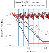
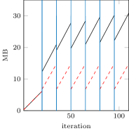
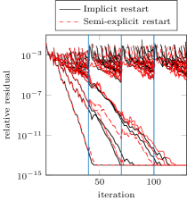
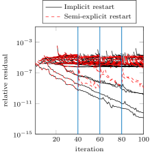
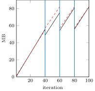
We now illustrate the differences between the semi–explicit and the implicit restart. More precisely, we show how the parameters $m$ and $p$ influence the convergence of the Ritz values with respect the number of iterations. The convergence of the semi–explicit restart appear to be slower in the semi–explicit restart when $p$ is not sufficiently large. See Figure 2a. The convergence speed of both restarting strategies is comparable for a larger $m$ and $p$. See Figure 3a.

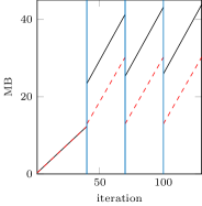
In practice, the performance of the two restarting strategies corresponds to a trade-off between CPU–time and memory. In particular, due to the fact that we impose the structure, the semi–explicit restart does not have a growth in the polynomial part at each restart and therefore requires less memory. On the other hand, for this problem, the semi–explicit restart appears to be slower in term of CPU–time. See Figure 2 and 3.

(a) Convergence

(b) Memory

Figure 2: Implicit and semi–explicit restart for DEP of size $n=40401$ with $m=20$, $p=5$ and restart=7

(a) Convergence

(b) Memory

Figure 3: Implicit and semi–explicit restart for DEP of size $n=40401$ with $m=40$, $p=10$ and restart=4

	Semi–explicit restart
	tensor structured functions		original approach Jarlebring2014Schur
Size	CPU	Memory	CPU	Memory
10201	19.07s	3.73 MB	31.41 s	65.38 MB
40401	30.14s	14.80 MB	1m30s	258.92 MB
160801	1m47s	58.89 MB	6m04	1.01 GB
641601	7m30s	234.96 MB	24m27s	4.02 GB
1002001	12m01s	366.94 MB	-	-

(a) $m=20$, $p=5$, restart=7

	Semi–explicit restart
	tensor structured functions		original approach Jarlebring2014Schur
Size	CPU	Memory	CPU	Memory
10201	13.47s	7.62 MB	1m05s	255.27 MB
40401	41.81s	30.20 MB	4m	1 GB
160801	144.79s	120.23 MB	15m54s	3.93 GB
641601	10m43s	479.71 MB	-	-
1002001	16m21s	749.18 MB	-	-

(b) $m=40$, $p=10$, restart=4

Table 1: Semi–explicit restart for DEP.

	Implicit restart
	compression		no compression
Problem size	CPU	Memory	CPU	Memory
10201	6.82s	7.78 MB	11.95s	17.12 MB
40401	21.96s	30.82 MB	37.63s	67.81 MB
160801	1m20s	120.23 MB	2m21s	269.90 MB
641601	5m24s	469.92 MB	9m33s	1.05 GB
1002001	8m36s	733.89 MB	15m16s	1.64 GB

(a) $m=20$, $p=5$, restart=7

	Implicit restart
	compression		no compression
Problem size	CPU	Memory	CPU	Memory
10201	9.54s	11.05 MB	16.61s	20.24 MB
40401	30.48s	43.76 MB	50.66s	80.14 MB
160801	1m54s	174.21 MB	3m11s	318.97 MB
641601	8m05s	695.09 MB	13m14s	1.24 GB
1002001	12m17s	1.06 GB	20m57s	1.94 GB

(b) $m=40$, $p=10$, restart=4

Table 2: Implicit restart for the DEP.

7.2 Waveguide eigenvalue problem

In order to illustrate how the performance depends on the problem properties, we now consider a NEP defined by functions with branch point and branch cut singularities. More precisely, we consider the waveguide eigenvalue problem (WEP) described in (WAVEGUIDE_ARNOLDI_2015, , Section 5.1) after the Cayley transformation. In this problem, $\Omega$ is the unit disc and there are branch point singularities in $\partial\Omega$. Thus, due to the slow convergence of the power series, in the semi–explicit restart we have to use (9) in order to compute $\mathbb{M}_{d}(Y,S)$. This also implies that the approximation by reducing the degree is not expected to be effective since the power series coefficients of $M(\lambda)$ are not decaying to zero.

In analogy to the previous subsection, we carried out numerical simulations in order to compare the semi–explicit and the implicit restart.

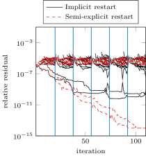
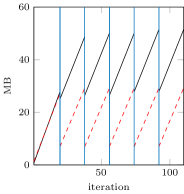
With Figure 4a and 5a, we illustrate the performance of the two restarting approaches with respect the choice of the parameters $m$ and $p$. When $p$ is sufficiently large, the residual in the semi–explicit restart appears to stagnate after the first restart whereas it decreases in a regular way in the implicit restart. See Figure 4a. On the other hand, when $p$ is small, the behavior of the residual appear to be specular. See Figure 5a. This is due to the fact that semi–explicit restart imposes the structure on $p$ vectors which is not beneficial when they do not contain eigenvector approximations.

It is known that this specific problem has two eigenvalues. Therefore, in order to reduce the CPU–time and the memory resources, the the number of wanted Ritz values $p$ should be selected small. As consequence of the above discussion, we conclude that the semi–explicit restart is the best restarting strategy for this problem.

(a) Convergence

(b) Memory

Figure 4: Implicit and semi–explicit restart for WEP of size $n=40803$ with $m=40$, $p=20$ and restart=4

(a) Convergence

(b) Memory

Figure 5: Implicit and semi–explicit restart for WEP of size $n=91203$ with $m=20$, $p=4$ and restart=6

	Implicit		Semi–explicit
Size	CPU	Memory	CPU	Memory
2703	5.33s	2.43 MB	13.02s	2.43 MB
10403	9.78s	9.36 MB	22.54s	9.36 MB
40803	29.15s	36.73 MB	1m14s	36.73 MB
161603	1m50s	143.02 MB	4m01s	145.48 MB
643203	7m27s	579.05 MB	17m44s	579.05 MB
1006009	11m54s	903.87 MB	27m55s	903.87 MB

(a) $m=20$, $p=4$, restart=6

	Implicit		Semi–explicit
Size	CPU	Memory	CPU	Memory
2703	5.09s	1.52 MB	5.17s	0.95 MB
10403	8.83s	5.87 MB	10.74s	3.65 MB
40803	25.93s	23.04 MB	24.11s	14.32 MB
161603	1m35s	91.24 MB	1m20s	56.71 MB
643203	6m31s	363.14 MB	5m44s	225.73 MB
1006009	10m25s	566.83 MB	8m57s	352.36 MB

(b) $m=40$, $p=20$, restart=4

Table 3: Implicit and semi–explicit restart for the waveguide problem.

8 Concluding remarks and outlook

In this work we have derived an extension of the TIAR algorithm and two restarting strategies. Both restarting strategies are based on approximating the TIAR factorization. In other works on the IAR–method it has been proven that the basis matrix contains a structure that allows exploitations, e.g. for NEPs with low rank structure in the coefficients van2016rank . An investigation about the combination of the approximations of the TIAR factorization with such structures of the NEP seems possible but deserve further attention.

Although the framework of TIAR and restarted TIAR is general, a specialization of the methods to the NEP is required in order to efficiently solve the problem. More precisely, an efficient computation procedure for computing (10) is required. This is a nontrivial task for many application and requires problem specific research.

References

- (1) M. Abramowitz, I. Stegun, Handbook of mathematical functions: with formulas, graphs, and mathematical tables, vol. 55, Courier Corporation, 1964.
- (2) Z. Bai, J. Demmel, J. Dongarra, A. Ruhe, H. van der Vorst, Templates for the solution of algebraic eigenvalue problems: a practical guide, vol. 11, Siam, 2000.
- (3) Z. Bai, Y. Su, Soar: A second-order Arnoldi method for the solution of the quadratic eigenvalue problem, SIAM J. Matrix Anal. Appl. 26 (3) (2005) 640–659.
- (4) B. Beckermann, The condition number of real vandermonde, Krylov and positive definite Hankel matrices, Numer. Math. 85 (4) (2000) 553–577.
- (5) R. V. Beeumen, K. Meerbergen, W. Michiels, Compact rational Krylov methods for nonlinear eigenvalue problems, SIAM J. Matrix Anal. Appl. 36 (2) (2015) 820––838.
- (6) M. M. Betcke, H. Voss, Restarting projection methods for rational eigenproblems arising in fluid-solid vibrations, Math. Model. Anal. 13 (2) (2008) 171–182.
- (7) M. M. Betcke, H. Voss, Restarting iterative projection methods for Hermitian nonlinear eigenvalue problems with minmax property, Numer. Math. (2016) 1–34.
- (8) T. Betcke, N. J. Higham, V. Mehrmann, C. Schröder, F. Tisseur, NLEVP: A collection of nonlinear eigenvalue problems, Tech. rep., Manchester Institute for Mathematical Sciences (2011).
- (9) T. Betcke, H. Voss, A Jacobi–Davidson-type projection method for nonlinear eigenvalue problems, Future Gener. Comp. Sy. 20 (3) (2004) 363–372.
- (10) C. Effenberger, Robust solution methods for nonlinear eigenvalue problems, Ph.D. thesis, École polytechnique fédérale de Lausanne (2013).
- (11) G. H. Golub, C. Van Loan, F. Charles, Matrix computations, vol. 3, JHU Press, 2012.
- (12) S. Gü˝̈ttel, R. Van Beeumen, K. Meerbergen, W. Michiels, NLEIGS: A class of fully rational Krylov methods for nonlinear eigenvalue problems, SIAM J. Sci. Comput. 36 (6) (2014) A2842–A2864.
- (13) E. Jarlebring, K. Meerbergen, W. Michiels, Computing a partial Schur factorization of nonlinear eigenvalue problems using the infinite Arnoldi method, SIAM J. Matrix Anal. Appl. 35 (2) (2014) 411–436.
- (14) E. Jarlebring, G. Mele, O. Runborg, The waveguide eigenvalue problem and the tensor infinite Arnoldi method, Tech. rep., arXiv:1503.02096 (2015).
- (15) E. Jarlebring, W. Michiels, K. Meerbergen, A linear eigenvalue algorithm for the nonlinear eigenvalue problem, Numer. Math. 122 (1) (2012) 169–195.
- (16) E. Jarlebring, F. Poloni, Iterative methods for the delay Lyapunov equation with T-Sylvester preconditioning, Tech. rep., arXiv:1507.02100 (2015).
- (17) D. Kressner, A block Newton method for nonlinear eigenvalue problems, Numer. Math. 114 (2) (2009) 355–372.
- (18) D. Kressner, J. E. Roman, Memory-efficient Arnoldi algorithms for linearizations of matrix polynomials in Chebyshev basis, Numer. Linear Algebra Appl. 21 (4) (2014) 569–588.
- (19) P. Lancaster, P. Psarrakos, On the pseudospectra of matrix polynomials, SIAM J. Matrix Anal. Appl. 27 (1) (2005) 115–129.
- (20) R. B. Lehoucq, Analysis and implementation of an implicitly restarted Arnoldi iteration, Ph.D. thesis, Rice University (1995).
- (21) R. B. Lehoucq, D. C. Sorensen, Deflation techniques for an implicitly restarted Arnoldi iteration, SIAM J. Matrix Anal. Appl. 17 (4) (1996) 789–821.
- (22) D. S. Mackey, N. Mackey, C. Mehl, V. Mehrmann, Structured polynomial eigenvalue problems: Good vibrations from good linearizations, SIAM J. Matrix Anal. Appl. 28 (4) (2006) 1029–1051.
- (23) D. S. Mackey, N. Mackey, F. Tisseur, Polynomial eigenvalue problems: Theory, computation, and structure, in: Numerical Algebra, Matrix Theory, Differential-Algebraic Equations and Control Theory, Springer, 2015, pp. 319–348.
- (24) K. Meerbergen, Locking and restarting quadratic eigenvalue solvers, SIAM J. Sci. Comput. 22 (5) (2001) 1814–1839.
- (25) K. Meerbergen, The quadratic Arnoldi method for the solution of the quadratic eigenvalue problem, SIAM J. Matrix Anal. Appl. 30 (4) (2008) 1463–1482.
- (26) V. Mehrmann, H. Voss, Nonlinear eigenvalue problems: A challenge for modern eigenvalue methods, GAMM-Mitt. 27 (2) (2004) 121–152.
- (27) R. Morgan, On restarting the Arnoldi method for large nonsymmetric eigenvalue problems, Math. Comp. 65 (215) (1996) 1213–1230.
- (28) A. Neumaier, Residual inverse iteration for the nonlinear eigenvalue problem, SIAM J. Numer. Anal. 22 (5) (1985) 914–923.
- (29) G. W. Stewart, A Krylov–Schur algorithm for large eigenproblems, SIAM J. Matrix Anal. Appl. 23 (3) (2002) 601–614.
- (30) Y. Su, Z. Bai, Solving rational eigenvalue problems via linearization, SIAM J. Matrix Anal. Appl. 32 (1) (2011) 201–216.
- (31) D. Szyld, E. Vecharynski, F. Xue, Preconditioned eigensolvers for large-scale nonlinear Hermitian eigenproblems with variational characterizations. II. Interior eigenvalues, SIAM J. Sci. Comput. 37 (6) (2015) A2969–A2997.
- (32) D. Szyld, F. Xue, Preconditioned eigensolvers for large-scale nonlinear Hermitian eigenproblems with variational characterizations. I. Extreme eigenvalues, Math. Comp. (2016) .
- (33) F. Tisseur, K. Meerbergen, The quadratic eigenvalue problem, SIAM Rev. 2 (2001) 235–286.
- (34) R. Van Beeumen, E. Jarlebring, W. Michiels, A rank-exploiting infinite Arnoldi algorithm for nonlinear eigenvalue problems, Numer. Linear Algebra Appl. (2016) .
- (35) H. Voss, A maxmin principle for nonlinear eigenvalue problems with application to a rational spectral problem in fluid-solid vibration, Appl. Math. 48 (6) (2003) 607–622.
- (36) H. Voss, An Arnoldi method for nonlinear eigenvalue problems, BIT 44 (2) (2004) 387–401.
- (37) H. Voss, Nonlinear eigenvalue problems, in: L. Hogben (ed.), Handbook of Linear Algebra, Second Edition, No. 164 in Discrete Mathematics and Its Applications, Chapman and Hall/CRC, 2013.
- (38) Y. Zhang, Y. Su, A memory-efficient model order reduction for time-delay systems, BIT 53 (4) (2013) 1047–1073.