Among-site variability in the stochastic dynamics of East African coral reefs

Abstract

Coral reefs are dynamic systems whose composition is highly influenced by unpredictable biotic and abiotic factors. Understanding the spatial scale at which long-term predictions of reef composition can be made will be crucial for guiding conservation efforts. Using a 22-year time series of benthic composition data from 20 reefs on the Kenyan and Tanzanian coast, we studied the long-term behaviour of Bayesian vector autoregressive state-space models for reef dynamics, incorporating among-site variability. We estimate that if there were no among-site variability, the total long-term variability would be approximately one third of its current value. Thus among-site variability contributes more to long-term variability in reef composition than does temporal variability. Individual sites are more predictable than previously thought, and predictions based on current snapshots are informative about long-term properties. Our approach allowed us to identify a subset of possible climate refugia sites with high conservation value, where the long-term probability of coral cover $\leq 0.1$ was very low. Analytical results show that this probability is most strongly influenced by among-site variability and by interactions among benthic components within sites. These findings suggest that conservation initiatives might be successful at the site scale as well as the regional scale.

Keywords

vector autoregressive model, state-space model, stochastic dynamics, community composition, spatial variability, temporal variability, coral reef, Bayesian statistics

Introduction

“Probabilistic language based on stochastic models of population growth” has been proposed as a standard way to evaluate conservation and management strategies (Ginzburg et al.,, 1982). For example, a stochastic population model can be used to estimate the probability of abundance falling below some critical level. Such population viability analyses are widely used, and may be reasonably accurate if sufficient data are available (Brook et al.,, 2000). In principle, the same approach could be used for communities, provided that a sufficiently simple model of community dynamics can be found.

A good candidate for such a model is the vector autoregressive model of order 1 or VAR(1) (Lütkepohl,, 1993; Ives et al.,, 2003). This is a discrete-time model for the vector of log abundances of a set of species or groups, which includes environmental stochasticity and may include environmental explanatory variables. It makes the simplifying assumptions that inter- and intraspecific interactions can be represented by a linear approximation on the log scale, and that future abundances are conditionally independent of past abundances, given current abundances. Where possible, it is desirable to use a state-space form of the VAR(1) model, which also includes measurement error (Lindegren et al.,, 2009; Mutshinda et al.,, 2009).

Hampton et al., (2013) review applications of VAR(1) models in community ecology, which include studying the stability of freshwater plankton systems (Ives et al.,, 2003), designing adaptive management strategies for the Baltic Sea cod fishery (Lindegren et al.,, 2009), and estimating the contributions of environmental stochasticity and species interactions to temporal fluctuations in abundance of moths, fish, crustaceans, birds and rodents (Mutshinda et al.,, 2009). Recently, VAR(1) models have been applied to the dynamics of the benthic composition of coral reefs (Cooper et al.,, 2015; Gross and Edmunds,, 2015), using a log-ratio transformation (Egozcue et al.,, 2003) rather than a log transformation, to deal with the constraint that proportional cover of space-filling benthic groups sums to 1.

Coral reefs are dynamic systems influenced by both deterministic factors such as interactions between macroalgae and hard corals (Mumby et al.,, 2007), and stochastic factors such as temperature fluctuations (Baker et al.,, 2008) and storms (Connell et al.,, 1997). In general, high coral cover is considered a desirable state for a coral reef, and there is some evidence that coral cover of at least 0.1 is important for long-term maintenance of reef function (Kennedy et al.,, 2013; Perry et al.,, 2013; Roff et al.,, 2015). Thus, coral cover of 0.1 might be an appropriate threshold against which to evaluate reef conservation strategies, and VAR(1) models can be used to estimate the probability of coral cover falling to or below this threshold (Cooper et al.,, 2015).

There is evidence for systematic differences in reef dynamics among locations. For example, on the Great Barrier Reef, coral cover has declined more strongly at southern and central than at northern sites (De’ath et al.,, 2012), and in the U.S. Virgin Islands, VAR(1) models showed that sites differed in their sensitivity to disturbance and speed of recovery (Gross and Edmunds,, 2015). Some sites in a region may therefore represent coral refugia, where reefs are either protected from or able to adapt to changes in environmental conditions (McClanahan et al.,, 2007). Although it may be possible to associate differences in dynamics among sites with differences in environmental variables, it is also possible to treat among-site differences as another random component of a VAR(1) model. This will allow estimation of the relative importance of among-site variability and within-site temporal variability, which is important for the design of conservation strategies. If within-site temporal variability dominates, it will not be possible to identify good sites to conserve based on current status, while if among-site variability dominates, even a “snapshot” sample at one time point may be enough to identify good sites. Thus, for example, the reliability of among-site patterns from surveys at one time point, such as the relationship between benthic composition and human impacts on remote Pacific atolls (Sandin et al.,, 2008), depends on among-site variability dominating within-site temporal variability. Furthermore, since among-site variability will affect the probability of undesirable community composition (such as coral cover $\leq 0.1$), conservation strategies that explicitly address among-site variability may be effective.

Here, we develop a state-space VAR(1) model for regional dynamics of East African coral reefs, including random site effects and measurement error, and use it to answer four key questions about spatial and temporal variability. How important is among-site variability in the dynamics of benthic composition, relative to within-site temporal variability? How much variability is there among sites in the probability of low ($\leq 0.1$) coral cover? What is the most effective way (in terms of altering model parameters) to reduce the probability of low coral cover in the region? How informative is a single snapshot in time about the long-term properties of a site?

Methods

Data collection

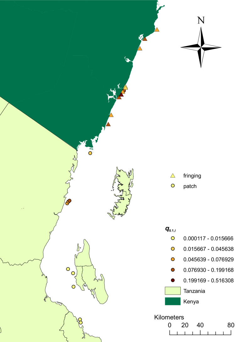
Figure A7: Map of study sites, showing fringing reefs (triangles) and patch reefs (circles), shaded by the site-specific long-term probability $q_{0.1,i}$ of coral cover $\leq 0.1$ (for reefs with one site) or the mean of site-specific probabilities (for reefs with two sites).

Surveys of 20 spatially distinct reefs in Kenya and Tanzania (supporting information, Table A1, Figure A7) were conducted annually during the period 1991-2013 (generally in November or December prior to 1998, but January or February from 1998 onwards). Those in the north were typically fringing reefs, $100\text{\,}\mathrm{m}2000\text{\,}\mathrm{m}$ from the shore, while those in the south were typically smaller and more isolated patch reefs, further from the shore (McClanahan and Arthur,, 2001). We categorized reefs as either fished or unfished, although there was substantial heterogeneity within these categories, because some fished reefs were community management areas with reduced harvesting intensity (Cinner and McClanahan,, 2015), and some unfished reefs had only recently been designated as reserves. Of the 20 reefs, 10 were divided into two sites separated by $20\text{\,}\mathrm{m}100\text{\,}\mathrm{m}$, while the remaining 10 reefs comprised only one site. The selection of sites represents available data rather than a random sample from all the locations at which coral reefs are present in the geographical area (and all of the longest time series are from Kenyan fringing reefs). Thus, when we refer below to ‘a randomly-chosen site’ we strictly mean ‘a site drawn at random from the population for which data could have been available.’

Each of the 30 sites was visited at least twice (data from sites visited once were omitted), with a maximum of 20 visits. A version of line-intercept sampling (Kaiser,, 1983; McClanahan et al.,, 2001) was used to estimate reef composition. In total, 2665 linear transects were sampled across all sites and years, with between 5 and 18 transects (median 9) at each site in a single year. Transects were randomly placed between two points $10\text{\,}\mathrm{m}$ apart, but as the transect line was draped over the contours of the substrate, the measured lengths varied between $10\text{\,}\mathrm{m}$ and $15\text{\,}\mathrm{m}$. Cover of benthic taxa was recorded as the sum of draped lengths of intersections of patches of each taxon with the line, divided by the total draped length of the line. Intersections with length less than $3\text{\,}\mathrm{cm}$ were not recorded. Taxa were identified to species or genus level, but for this study cover was grouped into three broad categories: hard coral, macroalgae and other (algal turf, calcareous and coralline algae, soft corals and sponges). Sand and seagrass were recorded, but excluded from our analysis, which focussed on hard substrate. The dynamics of a subset of these data were analyzed using different methods in Żychaluk et al., (2012).

Data processing

The three cover values form a three-part composition, a set of three positive numbers whose sum is 1 (Aitchison,, 1986, Definition 2.1, p. 26). Standard multivariate statistical techniques are not appropriate for untransformed compositional data, due to the absence of an interpretable covariance structure and the difficulties with parametric modelling (Aitchison,, 1986, chapter 3). To avoid these difficulties, the proportional cover data were transformed to orthogonal, unconstrained, isometric log-ratio (ilr) coordinates (Egozcue et al.,, 2003). The transformed data at site $i$, transect $j$, time $t$ were represented by the vector $\mathbf{y}_{i,j,t}=[y_{1,i,j,t},y_{2,i,j,t}]^{T}$, in which the first coordinate $y_{1,i,j,t}$ was proportional to the natural log of the ratio of algae to coral, and the second coordinate $y_{2,i,j,t}$ was proportional to the natural log of the ratio of other to the geometric mean of algae and coral (supporting information, section A1). The $T$ denotes transpose: throughout, we work with column vectors.

The model

The true value $\mathbf{x}_{i,t}=[x_{1,i,t},x_{2,i,t}]^{T}$ of the isometric log-ratio transformation of cover of hard corals, macroalgae and other at site $i$ at time $t$ was modelled by a vector autoregressive process of order 1 (i.e. a process in which the cover in a given year depends only on cover in the previous year), an approach used in other recent models of coral reef dynamics (Cooper et al.,, 2015; Gross and Edmunds,, 2015). Unlike previous models, we include a random term representing among-site variation, and explicit treatment of measurement error (making this a state-space model). The full model is

$$\mathbf{x}_{i,t+1} =\mathbf{a}+\bm{\alpha}_{i}+\mathbf{B}\mathbf{x}_{i,t}+\bm{\varepsilon}_{i,t},$$ (1)

$$\bm{\alpha}_{i} \sim\mathcal{N}(\mathbf{0},\mathbf{Z}),$$

$$\bm{\varepsilon}_{i,t} \sim\mathcal{N}(\mathbf{0},\bm{\Sigma})$$

$$\mathbf{y}_{i,j,t} \sim t_{2}(\mathbf{x}_{i,t},\mathbf{H},\nu).$$

The column vector $\mathbf{a}$ represents the among-site mean proportional changes in $\mathbf{x}_{i,t}$ evaluated at $\mathbf{x}_{i,t}=\mathbf{0}$. The column vector $\bm{\alpha}_{i}$ represents the amount by which these proportional changes for the $i$th site differ from the among-site mean, and is assumed to be drawn from a multivariate normal distribution with mean vector $\mathbf{0}$ and $2\times 2$ covariance matrix $\mathbf{Z}$. The $2\times 2$ matrix $\mathbf{B}$ represents the effects of $\mathbf{x}_{i,t}$ on the proportional changes, and can be thought of as summarizing intra- and inter-component interactions such as competition. The column vector $\bm{\varepsilon}_{i,t}$ represents random temporal variation, and is assumed to be drawn from a multivariate normal distribution with mean vector $\mathbf{0}$ and covariance matrix $\bm{\Sigma}$. We assume that there is no temporal or spatial autocorrelation in $\bm{\varepsilon}$, and that $\bm{\varepsilon}$ is independent of the among-site variation $\bm{\alpha}$.

The observed transformed compositions $\mathbf{y}_{i,j,t}$ vary around the corresponding true compositions $\mathbf{x}_{i,t}$ due to both small-scale spatial variation in true composition among transects within a site, and measurement error in estimating composition from a transect. We cannot easily separate these sources of variation because transects were located at different positions in each year, and there were no repeat measurements within transects. Observed log-ratio transformed cover $\mathbf{y}_{i,j,t}$ in the $j$th transect of site $i$ at time $t$ was assumed to be drawn from a bivariate $t$ distribution (denoted by $t_{2}$) with location vector equal to the corresponding $\mathbf{x}_{i,t}$, and unknown scale matrix $\mathbf{H}$ and degrees of freedom $\nu$ (Lange et al.,, 1989). The bivariate $t$ distribution can be interpreted as a mixture of bivariate normal distributions whose covariance matrices are the same up to a scalar multiple (Lange et al.,, 1989), and therefore allows a simple form of among-site or temporal variation in the distribution of measurement error or small-scale spatial variation, whose importance increases as the degrees of freedom decrease. Preliminary analyses suggested that it was important to allow this variation, because the model in Equation 1 fitted the data much better than a model with a bivariate normal distribution for $\mathbf{y}_{i,j,t}$ (supporting information, section A3).

We make the important simplifying assumptions that $\mathbf{B}$ is the same for all sites, and that the causes of among-site and temporal variation are not of interest. A separate $\mathbf{B}$ for each site, or even a hierarchical model for $\mathbf{B}$, would be difficult to estimate from the amount of data we have. It might be possible to explain some of the random temporal variation using temporally-varying environmental covariates such as sea surface temperature, and some of the among-site variation using temporally constant covariates such as management strategies (Cooper et al.,, 2015). However, it is not necessary to do so in order to answer the questions listed at the end of the introduction, and keeping the model as simple as possible is important because parameter estimation is quite difficult. Furthermore, some of the relevant environmental variables may be associated with management strategies, making it difficult to separate the effects of environmental variation and management. For example, although some water quality variables were not strongly associated with protection status (Carreiro-Silva and McClanahan,, 2012), unfished reefs were designated as protected areas due to their relatively good condition and are generally found in deeper lagoons with lower and more stable water temperatures than fished reefs (T. R. McClanahan, personal observation).

To understand the features of dynamics common to all sites, we plotted the back-transformations from ilr coordinates to the simplex of the overall intercept parameter $\mathbf{a}$ and the columns $\mathbf{a}_{1}$ and $\mathbf{a}_{2}$ of a matrix $\mathbf{A}$, which is related to $\mathbf{B}$ and describes the effects of current reef composition on the change in reef composition from year to year (Cooper et al.,, 2015). We plotted $\mathbf{A}$ rather than $\mathbf{B}$ because it leads to a simpler visualization of effects (supporting information, section A4). For example, a point lying to the left of the line representing equal proportions of coral and algae (the 1:1 coral-algae isoproportion line) corresponds to a parameter tending to increase coral relative to algae.

Parameter estimation

We estimated all model parameters and checked model performance using Bayesian methods implemented in the Stan programming language (Stan Development Team, 2015a, ), as described in the supporting information (section A5). Stan uses the No-U-Turn Sampler, a version of Hamiltonian Monte Carlo, which can converge much faster than random-walk Metropolis sampling when parameters are correlated (Hoffman and Gelman,, 2014). For most results, we report posterior means and $95\%$ highest posterior density (HPD) intervals (Hyndman,, 1996), calculated in R (R Core Team,, 2015).

Long-term behaviour

In the long term, the true transformed composition $\mathbf{x}^{*}$ of a randomly-chosen site will converge to a stationary distribution, provided that all the eigenvalues of $\mathbf{B}$ lie inside the unit circle in the complex plane (e.g. Lütkepohl,, 1993, p. 10). If the eigenvalues of $\mathbf{B}$ are complex, the system will oscillate as it approaches the stationary distribution. Details of long-term behaviour are in the supporting information, section A6.

This stationary distribution is the multivariate normal vector

$$\mathbf{x}^{*}\sim\mathcal{N}(\bm{\mu}^{*},\bm{\Sigma}^{*}+\mathbf{Z}^{*}),$$ (2)

whose stationary mean $\bm{\mu}^{*}$ depends on $\mathbf{B}$ and $\mathbf{a}$, and whose stationary covariance is the sum of the stationary within-site covariance $\bm{\Sigma}^{*}$ (which depends on $\mathbf{B}$ and $\bm{\Sigma}$) and the stationary among-site covariance $\mathbf{Z}^{*}$ (which depends on $\mathbf{B}$ and $\mathbf{Z}$).

For a fixed site $i$, the value of $\bm{\alpha}_{i}$ is fixed and the stationary distribution is given by

$$\mathbf{x}_{i}^{*}\sim\mathcal{N}(\bm{\mu}_{i}^{*},\bm{\Sigma}^{*}),$$ (3)

whose stationary mean $\bm{\mu}_{i}^{*}$ depends on $\mathbf{B}$, $\mathbf{a}$ and $\bm{\alpha}_{i}$, and whose stationary covariance matrix is $\bm{\Sigma}^{*}$. Note that $\mathbf{B}$, which describes intra- and inter-component interactions on an annual time scale, affects all the parameters of both stationary distributions, and therefore affects both within- and among-site variability in the long term. Also, the back-transformation of the stationary mean $\bm{\mu}^{*}$ of the transformed composition, rather than the arithmetic mean vector of the untransformed composition, is the appropriate measure of the centre of the stationary distribution (Aitchison,, 1989).

How important is among-site variability?

The covariance matrix of the stationary distribution for a randomly-chosen site (Equation 2) contains contributions from both among- and within-site variability. To quantify the contributions from these two sources, we calculated

$$\rho=\left(\frac{|\bm{\Sigma}^{*}|}{|\bm{\Sigma}^{*}+\mathbf{Z}^{*}|}\right)^{1/2},$$ (4)

(supporting information, section A7), which is the ratio of volumes of two unit ellipsoids of concentration (Kenward,, 1979), the numerator corresponding to the stationary distribution in the absence of among-site variation (or for a fixed site, as in Equation 3), and the denominator to the full stationary distribution of transformed reef composition in the region. The volume of each ellipsoid of concentration is a measure of the dispersion of the corresponding distribution. Thus $\rho$ provides an indication of how much of the total variability would remain if all among-site variability was removed. A similar statistic was used by Ives et al., (2003) to measure the contribution of species interactions to stationary variability.

How much variability is there among sites in the probability of low coral cover?

For a given coral cover threshold $\kappa$, we define $q_{\kappa,i}$ as the long-term probability that site $i$ has coral cover less than or equal to $\kappa$. This can be interpreted either as the proportion of time for which the site will have coral cover less than or equal to $\kappa$ in the long term, or as the probability that the site will have coral cover less than or equal to $\kappa$ at a random time, in the long term. We set $\kappa=0.1$, which has been suggested as a threshold for a positive net carbonate budget, based on simulation models and data from Caribbean reefs (Kennedy et al.,, 2013; Perry et al.,, 2013; Roff et al.,, 2015). We calculated $q_{0.1,i}$ for each site numerically (supporting information, section A8). In order to determine whether differences in $q_{0.1,i}$ were related to current coral cover, we plotted $q_{0.1,i}$ against the corresponding sample mean coral cover for each site, over all transects and years. In order to determine whether differences in $q_{0.1,i}$ had obvious explanations, we distinguished between fished and unfished reefs, and patch and fringing reefs. In order to determine whether there was strong spatial pattern in the probability of low coral cover, we calculated spline correlograms (Bjørnstad and Falck,, 2001) for a sample from the posterior distribution of $q_{0.1,i}$ (supporting information, section A9).

What is the most effective way to reduce the probability of low coral cover?

For a given coral cover threshold $\kappa$, we define $q_{\kappa}$ as the long-term probability that a randomly-chosen site has coral cover less than or equal to $\kappa$. This is equal to the expected long-term probability that coral cover is less than or equal to $\kappa$ over the region, and can be calculated numerically (supporting information, section A8). To find the most effective way to reduce $q_{\kappa}$, we calculated its derivatives with respect to each model parameter. As above, we concentrated on $\kappa=0.1$. However, we also compared results from $\kappa=0.05$ and $\kappa=0.20$. The probability $q_{\kappa}$ is a function of 12 parameters: all four elements of $\mathbf{B}$; both elements of $\mathbf{a}$; elements $\sigma_{11}$, $\sigma_{21}$ and $\sigma_{22}$ of $\bm{\Sigma}$; and elements $\zeta_{11}$, $\zeta_{21}$ and $\zeta_{22}$ of $\mathbf{Z}$. The negative of the gradient vector of derivatives of $q_{\kappa}$ with respect to these parameters describes the direction of movement through parameter space in which the probability of low coral cover will be reduced most rapidly, and the elements of this vector with the largest magnitudes correspond to the parameters to which $q_{\kappa}$ is most sensitive. To understand why $q_{\kappa}$ responds to each model parameter, note that $q_{\kappa}$ depends on the parameters $\bm{\mu}^{*}$, $\bm{\Sigma}^{*}$ and $\mathbf{Z}^{*}$ of the stationary distribution (Equation 2), which are in turn affected by the model parameters. We therefore used the chain rule for matrix derivatives (Magnus and Neudecker,, 2007, p.108) to break down the derivatives into effects of $\bm{\mu}^{*}$, $\bm{\Sigma}^{*}$ and $\mathbf{Z}^{*}$ on $q_{\kappa}$, and effects of model parameters on $\bm{\mu}^{*}$, $\bm{\Sigma}^{*}$ and $\mathbf{Z}^{*}$ (supporting information, section A10).

How informative is a snapshot about long-term site properties?

In a stochastic system, how much can a “snapshot” survey at a single point in time tell us about the long-term behaviour of the system? For example, are differences among sites that appear to be in good and bad condition likely to be maintained in the long term? To make this question more precise, suppose that we draw a site at random from the region, and at one point in time, draw the true state of the site at random from the stationary distribution for the site. This scenario matches Diamond’s definition of “natural snapshot experiments” as “comparisons of communities assumed to have reached a quasi-steady state” (Diamond,, 1986). For simplicity, we assume that we can estimate the true state accurately (for example, by taking a large number of transects). To quantify how informative this is about the long term properties of the site, we computed the correlation coefficients between corresponding components of the true state at a given site at a given time and of stationary mean for that site (supporting information, section A11). If these correlations are high, then a snapshot will be informative about long term properties.

Results

Overall dynamics

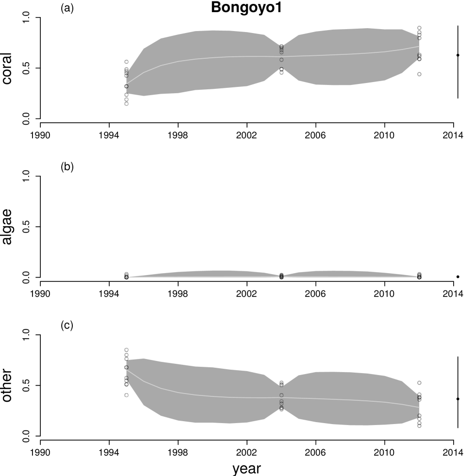
Figure A12: Time series for cover of hard corals (a), macroalgae (b) and other (c) at Bongoyo1. Circles are observations from individual transects. Grey lines join back-transformed posterior mean true states from Equation A.6 and the shaded region is a 95$\%$ HPD interval. The stationary mean composition for the site is the black dot after the time series and the bar is a 95$\%$ HPD interval.

At all sites, the model appeared to provide a good description of observed dynamics, although sometimes with high uncertainty. The back-transformed posterior mean true states from the model (e.g. Figure 1, grey lines) closely tracked the centres of the distributions of cover estimates from individual transects, although there was substantial among-transect variability at a given site in a given year (e.g. Figure 1, circles). Figure 1 shows two examples, and time series for all sites are plotted in the supporting information, Figures A12 to A41. There were also substantial differences in patterns of temporal change among sites. For example, Kanamai1 (Figure 1a-c), a fished site, had consistently low algal cover and no dramatic changes in cover of any component. In contrast, Mombasa1 (Figure 1d-f), an unfished site, had a sudden decrease in coral cover in 1998, and algal cover was high from 2007 onwards. As a result, Mombasa1 was unusual in that the current estimate of true algal cover was well above the stationary mean estimate (Figure 1e: black circle at end of time series). For most other sites, current estimated true cover was close to the stationary mean (supporting information, Figures A12 to A41, black circles at ends of time series). The uncertainty in true states (Figure 1, grey polygons represent $95\%$ highest posterior density (HPD) credible intervals) was higher during intervals with missing observations (e.g. 2008 in Figure 1). In general, uncertainty in true states (grey polygons) and stationary means (black bars at end of time series) was highest for sites with few observations (e.g. Bongoyo1, Figure A12).

The overall intercept parameter $\mathbf{a}$ (Figure 2, green), which describes the dynamics of reef composition at the origin (where each component is equally abundant) was consistent with the observed low macroalgal cover in the region (e.g. Figure 1b, e). The back-transformation of $\mathbf{a}$ lay close to the coral-other edge of the ternary plot, and slightly above the 1:1 coral-other isoproportion line. It therefore represented a strong year-to-year decrease in algae, and a slight increase in other relative to coral, at the origin.

Current reef composition acts on year-to-year change in composition (through matrix $\mathbf{A}$) so as to maintain fairly stable reef composition. The first column $\mathbf{a}_{1}$ of $\mathbf{A}$, which represents the effects of the transformed ratio of algae to coral on year-to-year change in composition, lay (when back-transformed) to the left of the 1:1 coral-algae isoproportion line, above the 1:1 other-algae isoproportion line, and below the 1:1 coral-other isoproportion line (Figure 2, orange). Thus, increases in algae relative to coral resulted in decreases in algae relative to coral and other, and increases in coral relative to other, in the following year. The second column $\mathbf{a}_{2}$ of $\mathbf{A}$, which represents the effects of the transformed ratio of other to algae and coral on year-to-year change in composition, lay (when back-transformed) on the 1:1 coral-algae isoproportion line, below the 1:1 other-algae isoproportion line, and below the 1:1 coral-other isoproportion line (Figure 2, blue). Thus, increases in other relative to algae and coral resulted in little change in the ratio of coral to algae, but decreases in other relative to both coral and algae. Consistent with the above interpretation of year-to-year dynamics, every set of parameters in the Monte Carlo sample led to a stationary distribution, since both eigenvalues of $\mathbf{B}$ lay inside the unit circle in the complex plane (supporting information, section A12). The magnitudes of these eigenvalues were smaller than those for a similar model for the Great Barrier Reef (Cooper et al.,, 2015), indicating more rapid approach to the stationary distribution. There was some evidence for complex eigenvalues of $\mathbf{B}$, leading to rapidly-decaying oscillations in both components of transformed reef composition on approach to this distribution. This contrasts with the Great Barrier Reef, where there was no evidence for oscillations (Cooper et al.,, 2015).

How important is among-site variability?

There was substantial among-site variability in the locations of stationary means (Figure 3, dispersion of points). Stationary mean algal cover was always low, but there was a wide range of stationary mean coral cover. Although our primary focus is not on the causes of among-site variability, there was a tendency for most of the reefs with highest stationary mean coral cover to be patch reefs (Figure 3, circles). The stationary means did not clearly separate by management (Figure 3, open symbols fished, filled symbols unfished). The long-term temporal variability around the stationary means was also substantial (Figure 3, green lines), as was the uncertainty in the values of the stationary means (Figure 3, grey dashed lines). The $\rho$ statistic (Equation 4), which quantifies the posterior mean contribution of within-site variability to the total stationary variability in reef composition in the region, was 0.29 ($95\%$ HPD interval $[0.20,0.39]$), or approximately one third. Thus, while within-site temporal variability around the stationary mean was not negligible, among-site variability in the stationary mean was more important in the long term.

For all three components of variability (within-site, among-site, and measurement error/small-scale spatial variability), variation in algal cover was larger than variation in coral or other. This can be seen in the shapes of the back-transformed unit ellipsoids of concentration (Figure 4: within-site, green; among-site, orange; measurement error and small-scale spatial variability, blue) which were all elongated to some extent along the 1:1 coral-other isoproportion line. This was similar to, but less extreme than, the pattern observed in the Great Barrier Reef (Cooper et al.,, 2015). The among-site ellipsoid almost entirely enclosed the within-site ellipsoid, consistent with the estimate above that among-site variability was more important than within-site variability in the long term. The large estimated measurement error/small-scale spatial variability component was consistent with the substantial observed variability in cover among transects at any given site and time (Figure 1, circles and supporting information, Figures A12 to A41, circles). The low estimated degrees of freedom $\nu$ for the bivariate $t$ distribution of measurement error/small-scale spatial variability (posterior mean 2.99, $95\%$ HPD interval $[2.64,3.35]$) suggested that some aspect of the process leading to variation in measured composition among transects at a given site was varying substantially over space or time, although we cannot determine the mechanism.

How much variability is there among sites in the probability of low coral cover?

There was also substantial among-site variability in the probability of low coral cover. For a randomly-chosen site, the posterior mean probability of coral cover less than or equal to 0.1 ($q_{0.1}$) in the long term was 0.12 ($95\%$ credible interval $[0.04,0.21]$). The corresponding site-specific probabilities $q_{0.1,i}$ varied from $8\times 10^{-5}$ to 0.52 but were low for most sites, with a strong negative relationship between probability of low coral cover and observed mean coral cover (Figure 5). There was no clear distinction between fished and unfished reefs (Figure 5, open symbols fished, filled symbols unfished). However, probability of low coral cover appeared to be systematically lower on patch reefs, which were mainly in Tanzania (Figures 5 and A7, circles: median of posterior means $2\times 10^{-3}$, first quartile $4\times 10^{-4}$, third quartile 0.04) than on fringing reefs (Figures 5 and A7, triangles: median of posterior means 0.08, first quartile 0.04, third quartile 0.11). One site (Ras Iwatine) had a much higher probability of low coral cover than all others, and is relatively polluted compared to other sites in this study, due to high levels of nutrient effluent from a large hotel (T.R. McClanahan, personal observation).

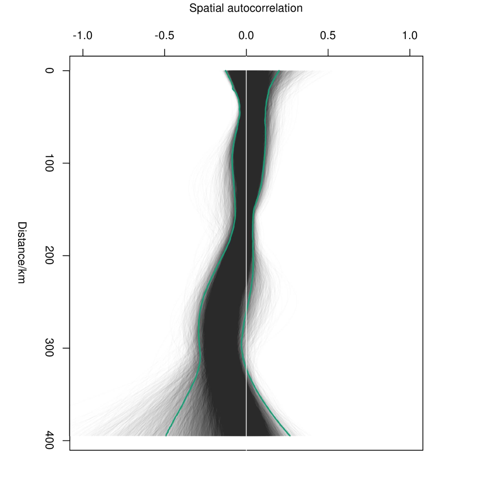
Figure A44: Spline correlogram of spatial autocorrelation in $q_{0,1,i}$. Grey lines: spline correlograms from each of 20000 Monte Carlo iterations. Thick green lines: $95\%$ highest posterior density envelope. White horizontal line: zero-correlation reference line.

There was little evidence for strong spatial autocorrelation in the probability of low coral cover, because the $95\%$ envelope for the spline correlogram included zero for all distances other than $261\text{\,}\mathrm{km}322\text{\,}\mathrm{km}$ (supporting information, Figure A44). The general lack of strong spatial autocorrelation reflects the substantial variation in probability of coral cover less than or equal to 0.1 ($q_{0.1,i}$) among nearby sites, while the possibility of negative spatial autocorrelation at scales of around $300\text{\,}\mathrm{km}$ may reflect the generally low values of $q_{0.1,i}$ for Tanzanian patch reefs, separated from sites in the north of the study area with generally higher $q_{0.1,i}$ by approximately $300\text{\,}\mathrm{km}$ (Figure A7).

What is the most effective way to reduce the probability of low coral cover?

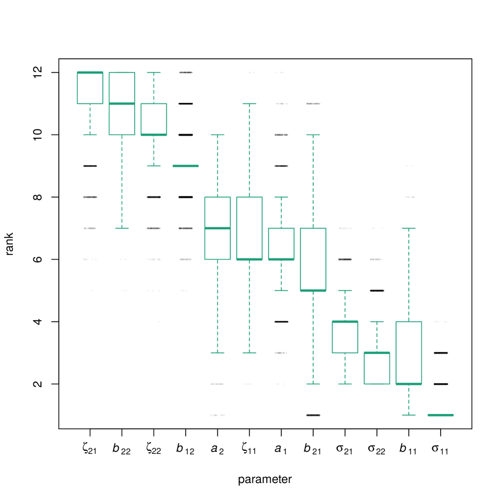
Figure A45: Ranks of partial derivatives of the long-term probability of coral cover less than or equal to 0.1 with respect to elements of the $\mathbf{B}$ matrix, the $\mathbf{a}$ vector, the covariance matrix of random temporal variation $\bm{\Sigma}$, and the covariance matrix of among-site variability $\mathbf{Z}$. Parameters are ranked in descending order of median rank (higher ranks indicate larger magnitudes of partial derivative). Outliers are indicated as jittered black dots. For the covariance matrices, the elements $\sigma_{12}$ and $\zeta_{12}$ are not shown, because they are constrained to be equal to $\sigma_{21}$ and $\zeta_{21}$ respectively.

Both among-site variability and internal dynamics, particularly of other relative to algae and coral (component 2), were important in determining the probability $q_{0.1}$ of coral cover $\leq 0.1$ in the region. Figure 6 shows the direction in parameter space along which the probability of low coral cover will reduce most rapidly (the estimated gradient vector of $q_{0.1}$ with respect to all the model parameters). The four parameters to which $q_{0.1}$ was most sensitive were (in descending order: Figure 6) $\zeta_{21}$ (among-site covariance between transformed components 1 and 2), $b_{22}$ (effect of component 2 on next year’s component 2), $\zeta_{22}$ (among-site variance of component 2), and $b_{12}$ (effect of component 2 on next year’s component 1). Although there was substantial variability among Monte Carlo iterations in the values of these derivatives, the rank order of magnitudes was fairly consistent (supporting information, Figure A45). All four most important parameters had positive effects on $q_{0.1}$ (Figure 6), so reducing these parameters will reduce $q_{0.1}$. The effects of within-site temporal variability on the probability of low coral cover were relatively unimportant (Figure 6, derivatives of $q_{0.1}$ with respect to $\sigma_{11}$, $\sigma_{21}$ and $\sigma_{22}$ all had posterior means close to zero). The signs of the effects of each parameter on $q_{0.1}$, and results for coral cover thresholds 0.05 and 0.1, are discussed further in the supporting information (sections A13 and A14).

How informative is a snapshot about long-term site properties?

For both components of transformed composition, a snapshot of reef composition at a single time on a randomly-chosen site will be informative about the stationary mean (correlations between true value at a given time and stationary mean: component 1 posterior mean 0.84, 95$\%$ HPD interval $[0.75,0.91]$; component 2 posterior mean 0.82, 95$\%$ HPD interval $[0.73,0.90]$). This is consistent with the negative relationship between long-term probability of coral cover $\leq 0.1$ and observed mean coral cover (Figure 5). Thus, while long-term monitoring of East African coral reefs is important for other reasons, it should be possible to identify those with high conservation value (in terms of benthic composition) from a single survey.

Discussion

In the long term, among-site variability dominates within-site temporal variability in East African coral reefs. In consequence, the long-term probability of coral cover $\leq 0.1$ varied substantially among sites. This suggests that it is in principle possible to make reliable decisions about the conservation value of individual sites based on a survey of multiple sites at one point in time, and to design conservation strategies at the site level. This was not the only possible outcome: if within-site temporal variability dominated among-site variability, among-site differences would be neither important nor predictable in the long term. Given the large positive effect of among-site variability on the long-term probability of coral cover $\leq 0.1$, reducing among-site variability in compositional dynamics may be an effective conservation strategy.

The dominance of among-site variability has important implications for conservation. There was clear evidence for the existence of a stationary distribution of long-term reef composition in East Africa. The overall shape of this distribution (Figure 3) was similar to that estimated by Żychaluk et al., (2012) for a subset of the same data, using a different modelling approach. However, our new analysis shows that this distribution is generated by a combination of spatial and temporal processes, with substantial long-term differences among sites. Thus, the distribution in Żychaluk et al., (2012) may be a good approximation to the long-term distribution for a randomly-chosen site, but there will be much less variability over time in the distribution for any fixed site. In consequence, the sites having the highest long-term conservation value can be identified even from single-survey snapshots, and conservation strategies at the site scale may be possible. Furthermore, in cases where among-site variability in dynamics is dominant, it will be misleading to generalize from observations of a few sites to regional patterns (Bruno et al.,, 2009).

In our study, the sites with the highest long-term conservation value are those with very low long-term probabilities of coral cover $\leq 0.1$ (Figure 5), a threshold chosen based on evidence that coral cover $\leq 0.1$ is detrimental to reef persistence (Kennedy et al.,, 2013; Perry et al.,, 2013; Roff et al.,, 2015). Many of these sites are Tanzanian patch reefs, which may have maintained high coral cover despite disturbance because of local hydrography (McClanahan et al.,, 2007), and are priority sites for conservation, with high alpha and beta diversity (Ateweberhan and McClanahan,, 2016). In the light of these observations, we experimented with a model in which reef type was included as an explanatory variable. Although the estimated effects of reef type were consistent with lower long-term probabilities of coral cover $\leq 0.1$, including reef type did not improve the expected predictive accuracy of the model (F. Chong, unpublished results), probably because only 482 out of 2665 transects were from patch reefs, and all but one patch reefs had only very short time series (supporting information, Table A1). Furthermore, the absence of strong spatial autocorrelation in long-term probabilities of coral cover $\leq 0.1$ suggests that it will be necessary to consider conservation value at small spatial scales, rather than simply to identify subregions with high conservation value. Similarly, Vercelloni et al., (2014) found that trajectories of coral cover on the Great Barrier Reef were consistent at the scale of $\mathrm{k}\mathrm{m}^{2}$, but not at larger spatial scales. They argued that it would therefore be appropriate to focus management actions at the $\mathrm{k}\mathrm{m}^{2}$ scale. Also, it may be easier to persuade local communities to accept management at such scales than at larger scales (McClanahan et al.,, 2016).

A key result is that if we want to minimize the long-term probability $q_{0.1}$ that a randomly-chosen site has coral cover $\leq 0.1$, we should minimize among-reef variability in dynamics, other things being equal. This is because the centre of the stationary distribution lies outside the set of compositions with coral cover $\leq 0.1$ (Supporting Information, Section A13). Conversely, if the centre lay inside this set, then (other things being equal) maximizing among-site variability would minimize $q_{0.1}$. This result is very general, applying to any model of community composition which has a stationary distribution, for which increasing among-site variability increases stationary variability, and for any conservation objective based on a composition threshold.

Conservation strategies that might minimize among-site variability include distributing a fixed amount of human activity such as coastal development or fishing evenly, rather than concentrating it in a few locations. On the other hand, many conservation strategies will affect both the mean dynamics and the among-site variability in dynamics. For example, protecting the sites that are already in the best condition will tend to increase among-site variability, while moving the centre of the stationary distribution away from the set of compositions with coral cover $\leq 0.1$.

Minimizing among-site variability in dynamics may conflict with other proposed conservation strategies. It has been suggested that increased beta diversity is associated with lower temporal variability in metacommunities, for at least some taxa, and that regions of high beta diversity may therefore be priority regions for conservation (Mellin et al.,, 2014). It is likely that increased beta diversity will also be associated with increased among-site variability in dynamics, because different species are likely to have different population-dynamic characteristics. Hence, it may not always be possible to manage for both low among-site variability in dynamics and high beta diversity. It is not yet clear which of these objectives is more important in general.

Our analyses were based on the long-term consequences of current environmental conditions, and may therefore not be relevant if environmental conditions change. For example, if changes in climate or local human activity altered the vector $\mathbf{a}$ so as to transpose the centre of the stationary distribution into the set with coral cover $\leq 0.1$, then maximizing among-site variability would become the best strategy. Since declining coral cover trends have been observed at the regional level (e.g. Côté et al.,, 2005; De’ath et al.,, 2012), such a shift in the best strategy may occur. It is therefore better to view a stationary distribution under current conditions as a “speedometer” that tells us about the long-term outcome if these conditions were maintained, rather than as a prediction (Caswell,, 2001, p. 30).

In conclusion, our analysis extends the broadly-applicable vector autoregressive approach to community dynamics (reviewed by Hampton et al.,, 2013) by quantifying random among-site variability in dynamics. This gives a new perspective on the long-term behaviour of the set of communities in a region, as a set of stationary distributions with random but persistent differences. The extent of these differences relative to temporal variability determines how predictable the behaviour of individual sites will be. Since these differences may be associated with differences in conservation value, probabilistic risk assessment based on this approach can be used to suggest conservation strategies at both site and regional scales. At site scales, our approach can be used to identify potential coral refugia, while at regional scales, it can identify the parameters with most influence on conservation objectives.

Figure legends

Figure 1. Time series of cover of hard corals, macroalgae and other at two of the 30 sites surveyed: Kanamai1 (fished, a-c) and Mombasa1 (unfished, d-f). Circles are observations from individual transects. Grey lines join back-transformed posterior mean true states from Equation 1, and the shaded region is a 95$\%$ highest posterior density interval. The back-transformed stationary mean composition for the site is the black dot after the time series and the bar is a 95$\%$ highest posterior density interval.

Figure 2. Posterior distributions of the back-transformed overall intercept $\mathbf{a}$ (green), effect $\mathbf{a}_{1}$ of component 1 (proportional to log(algae/coral)) on year-to-year change (orange), and effect $\mathbf{a}_{2}$ of component 2 (proportional to log(other/geometric mean(algae,coral)) on year-to-year change (blue).

Figure 3. Stationary among- and within-site variation in benthic composition. Grey points: back-transformed stationary means for each site (open circles fished patch, filled circles unfished patch, open triangles fished fringing, filled triangles unfished fringing, posterior means of of stationary means). Grey dashed curves: back-transformed unit ellipsoids of concentration representing uncertainty in stationary means (calculated using sample covariance matrices from Monte Carlo iterations). Green solid curves: back-transformed unit ellipsoids of concentration representing within-site stationary variation (calculated using posterior mean within-site covariance matrix).

Figure 4. Back-transformed unit ellipsoids of concentration for stationary within-site covariance $\bm{\Sigma}^{*}$ (green), stationary among-site covariance $\mathbf{Z}^{*}$ (orange), and measurement error/small-scale spatial variation $\nu\mathbf{H}/(\nu-2)$ (blue). In each case, 200 ellipsoids drawn from the posterior distribution are plotted, centred on the origin.

Figure 5. Long-term probability of coral cover less than or equal to 0.1 at each site against mean observed coral cover across all years. Circles are patch reefs and triangles are fringing reefs. Open symbols are fished reefs and shaded symbols are unfished. Vertical lines are 95$\%$ highest posterior density intervals.

Figure 6. Elements of the gradient vector of partial derivatives of the long-term probability of coral cover less than or equal to 0.1 with respect to elements of the $\mathbf{B}$ matrix (effects of transformed composition in a given year on transformed composition in the following year), the $\mathbf{a}$ vector (overall intercept, representing among-site mean proportional changes in transformed composition at the origin), the covariance matrix of random temporal variation $\bm{\Sigma}$, and the covariance matrix of among-site variability $\mathbf{Z}$. For each parameter, the dot is the posterior mean and the bar is a 95$\%$ highest posterior density credible interval. For the covariance matrices, the elements $\sigma_{12}$ and $\zeta_{12}$ are not shown, because they are constrained to be equal to $\sigma_{21}$ and $\zeta_{21}$ respectively. The horizontal dashed line is at zero, the no-effect value.

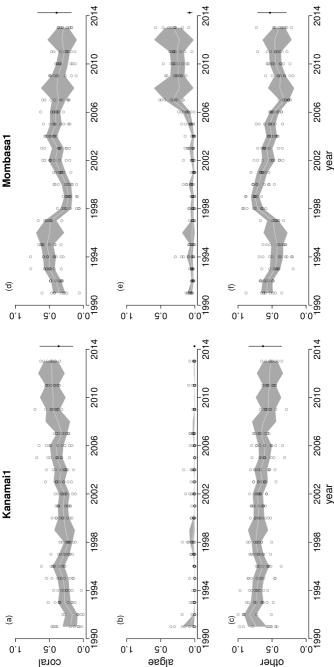
Figure 1:

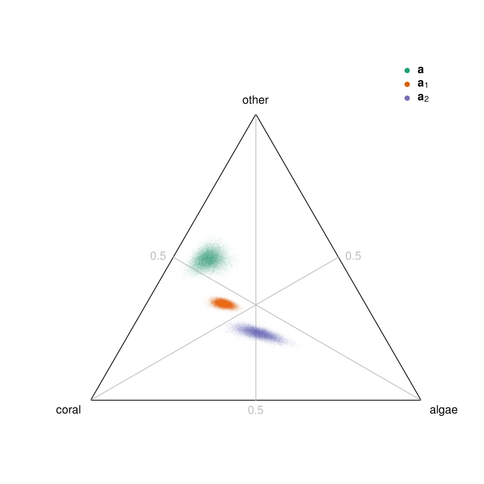
Figure 2:

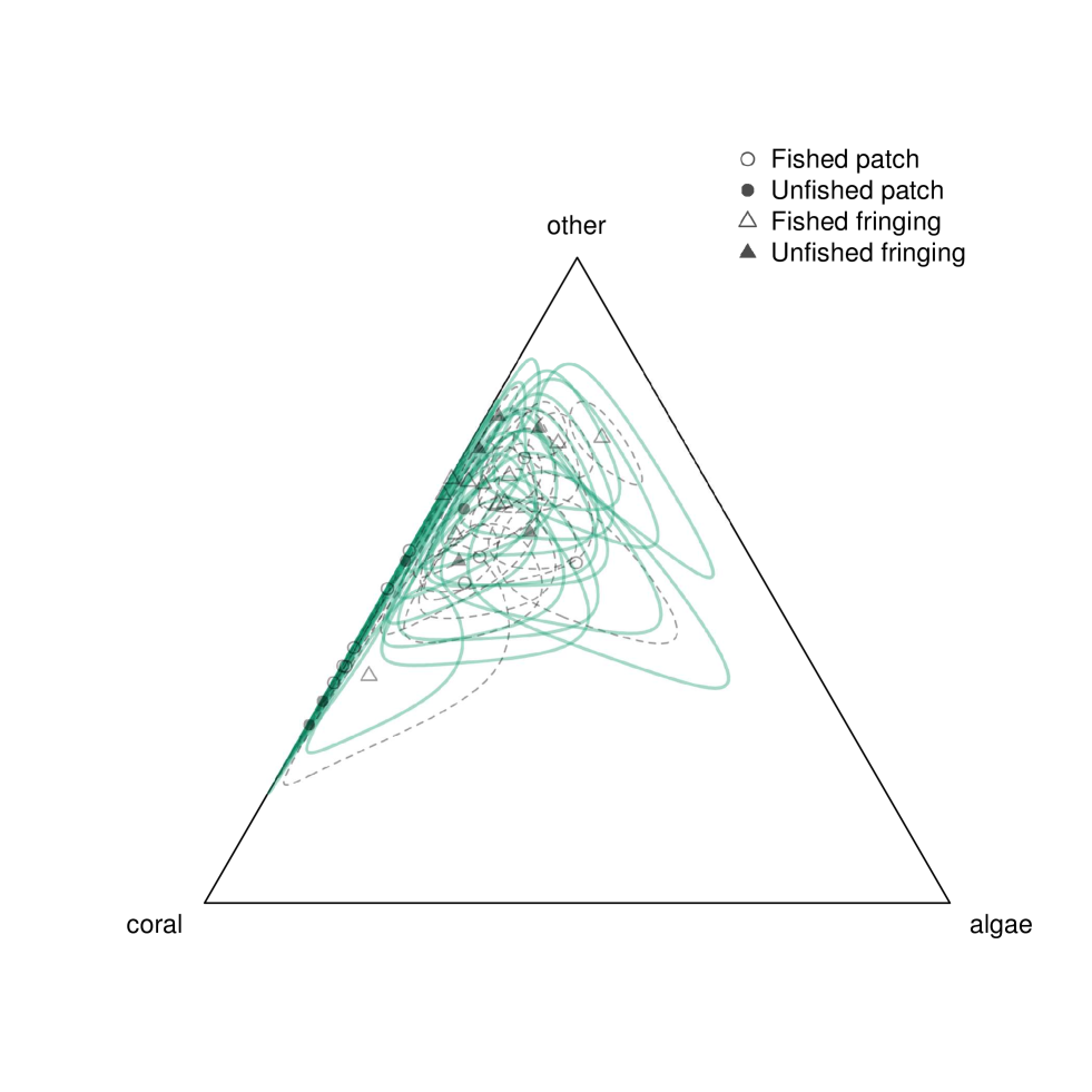
Figure 3:

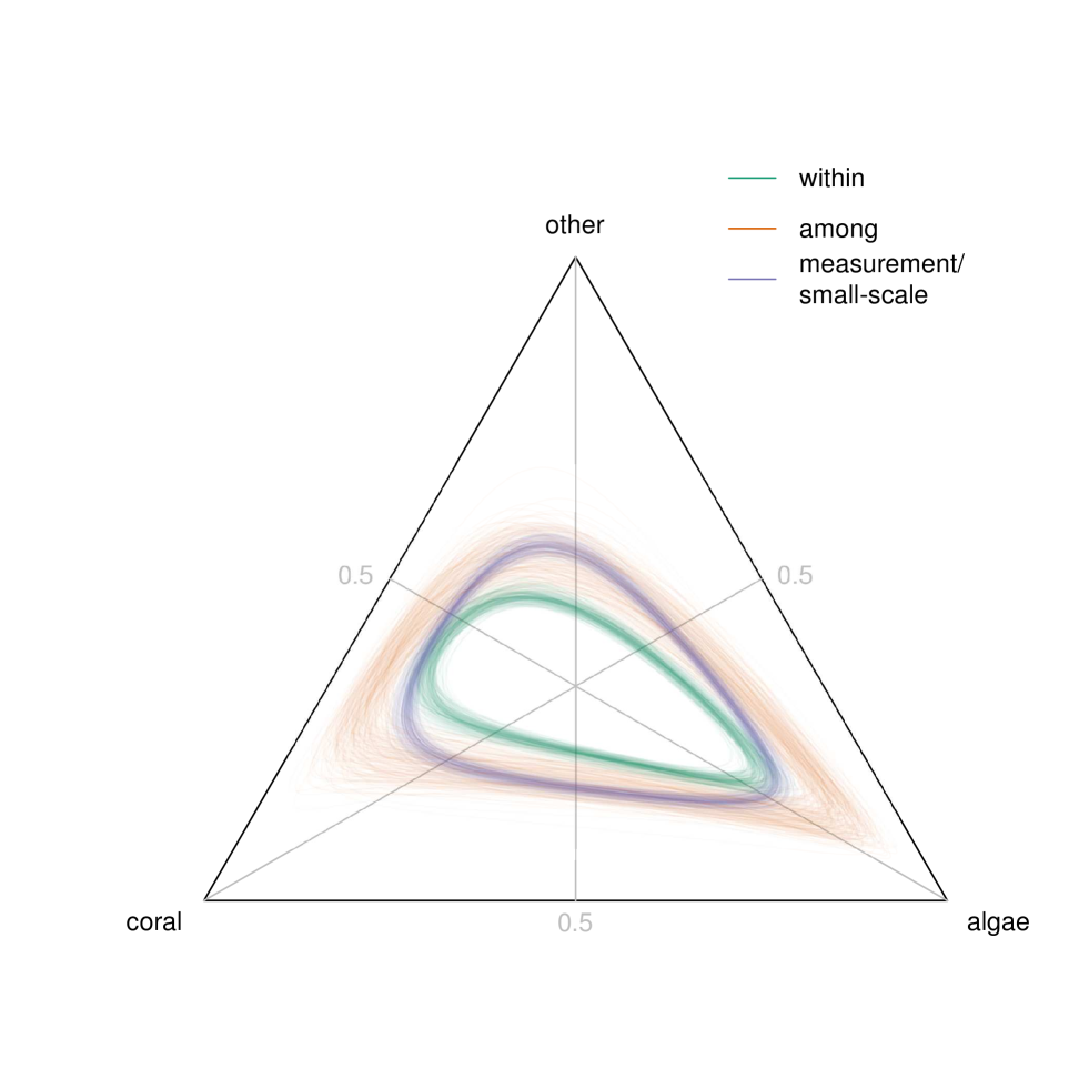
Figure 4:

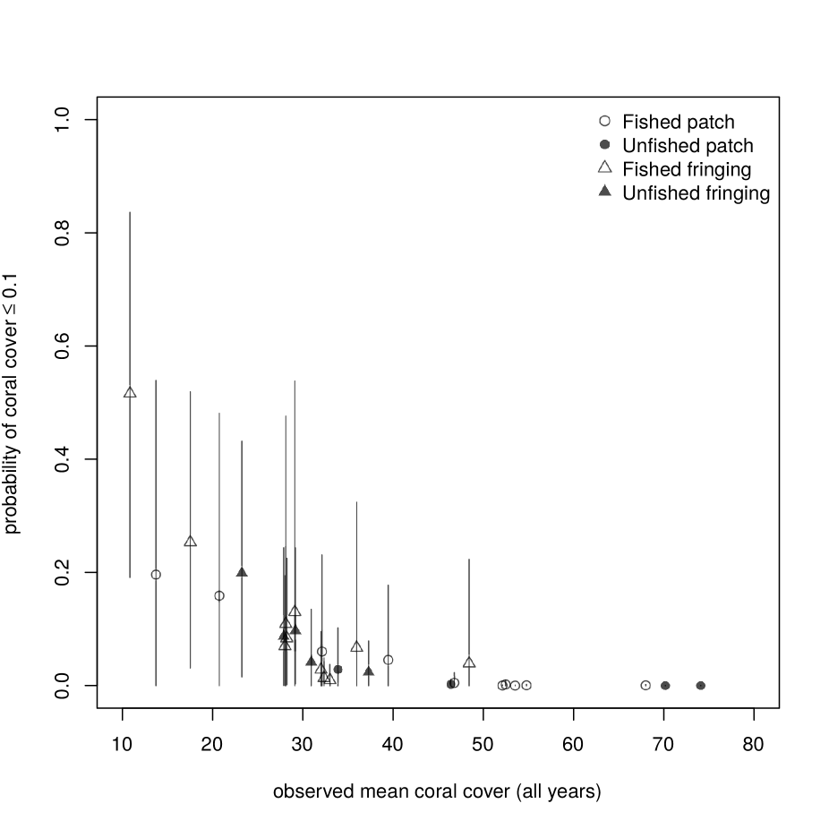
Figure 5:

Figure 6:

A1 Data transformation

Proportional cover data were transformed to isometric log-ratio (ilr) coordinates (Egozcue et al.,, 2003). Let $\mathbf{z}_{i,j,t}=[z_{1,i,j,t},z_{2,i,j,t},z_{3,i,j,t}]^{T}$ denote a vector of observed proportional cover of coral ($z_{1,i,j,t}$), algae ($z_{2,i,j,t}$) and other ($z_{3,i,j,t}$) at site $i$, transect $j$, at time $t$ (the $T$ denotes transpose). Then the ilr transformation for our data is given by

$$\mathrm{ilr}\colon\mathbb{S}^{3} \to\mathbb{R}^{2},$$ (A.5)

$$\mathbf{z}_{i,j,t}=[z_{1,i,j,t},z_{2,i,j,t},z_{3,i,j,t}]^{T} \mapsto\left[\frac{1}{\sqrt{2}}\log\left(\frac{z_{2,i,j,t}}{z_{1,i,j,t}}\right),\frac{2}{\sqrt{6}}\log\left(\frac{z_{3,i,j,t}}{\sqrt{z_{1,i,j,t}z_{2,i,j,t}}}\right)\right]^{T},$$

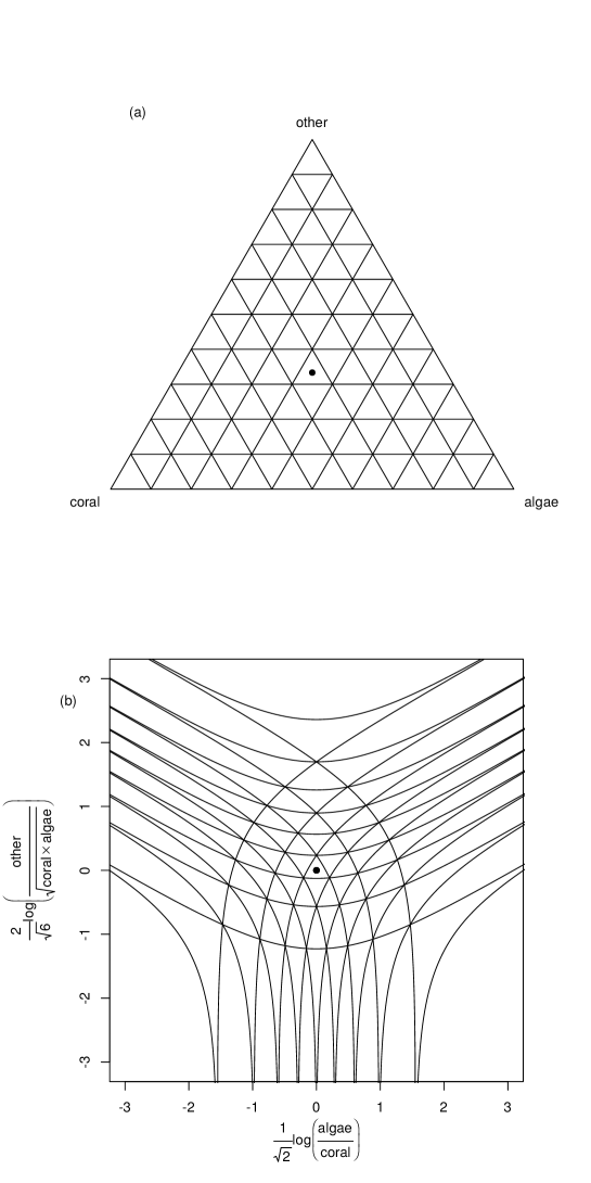
Figure A8: The ilr transformation given by Equation A.5. (a) The open 2-simplex $\mathbb{S}^{3}$, in which three-part compositions lie. The dot represents the composition with equal relative abundances of coral, algae and other. Lines are contours of constant relative abundance of one part. (b) The ilr-transformed composition in $\mathbb{R}^{2}$, with dot and contours as in (a).

where $\mathbb{S}^{3}$ denotes the open 2-simplex in which three-part compositions lie. The first element of the transformed composition is proportional to the natural log of the ratio of algae to coral, and the second element is proportional to the natural log of the ratio of other to the geometric mean of algae and coral. The transformation can be thought of as stretching out the open 2-simplex (Figure A8(a)) so that it covers the whole of the real plane (Figure A8(b)).

As the domain of the transformation is the open simplex, which does not include compositions with zero parts, any observed zeros were replaced by half the smallest non-zero value recorded (0.0008) before transformation, and the other components rescaled accordingly. This is the simple replacement strategy described in Martín-Fernández et al., (2003), although more sophisticated approaches are possible. We denote the resulting transformed observations by $\mathbf{y}_{i,j,t}=[y_{1,i,j,t},y_{2,i,j,t}]^{T}$.

A2 The model

For convenience, we reproduce the full model equations here:

$$\mathbf{x}_{i,t+1} =\mathbf{a}+\bm{\alpha}_{i}+\mathbf{B}\mathbf{x}_{i,t}+\bm{\varepsilon}_{i,t},$$ (A.6)

$$\bm{\alpha}_{i} \sim\mathcal{N}(\mathbf{0},\mathbf{Z}),$$

$$\bm{\varepsilon}_{i,t} \sim\mathcal{N}(\mathbf{0},\bm{\Sigma})$$

$$\mathbf{y}_{i,j,t} \sim t_{2}(\mathbf{x}_{i,t},\mathbf{H},\nu),$$

where $\mathbf{x}_{i,t}$ is the true transformed composition at site $i$, time $t$, $\mathbf{a}$ is a vector of among-site mean proportional changes evaluated at $\mathbf{x}_{i,t}=\mathbf{0}$, $\bm{\alpha}_{i}$ represents the amount by which these proportional changes for the $i$th site differ from the among-site mean, the $2\times 2$ matrix $\mathbf{B}$ represents the effects of $\mathbf{x}_{i,t}$ on the proportional changes, $\bm{\varepsilon}_{i,t}$ represents random temporal variation,

$$\mathbf{Z}=\begin{bmatrix}\zeta_{11}&\zeta_{12}\\ \zeta_{21}&\zeta_{22}\end{bmatrix}$$

is the covariance matrix of the among-site term $\bm{\alpha}_{i}$ (note that throughout, a diagonal element such as $\zeta_{ii}$ of a covariance matrix represent the variance of the $i$th variable),

$$\mathbf{\Sigma}=\begin{bmatrix}\sigma_{11}&\sigma_{12}\\ \sigma_{21}&\sigma_{22}\end{bmatrix}$$

is the covariance matrix of the temporal variation, $\mathbf{y}_{i,j,t}$ is the observed log-ratio transformed cover in the $j$th transect of site $i$ at time $t$,

$$\mathbf{H}=\begin{bmatrix}\eta_{11}&\eta_{12}\\ \eta_{21}&\eta_{22}\end{bmatrix}$$

is the scale matrix of the bivariate $t$ distribution of the $\mathbf{y}_{i,j,t}$, and $\nu$ is the corresponding degrees of freedom.

A3 Describing measurement error and small-scale temporal variability

We initially considered using a bivariate normal distribution to describe the variability of observed transformed composition $\mathbf{y}_{i,j,t}$ around true composition $\mathbf{x}_{i,t}$, but preliminary analyses showed that a heavier-tailed distribution was needed. We therefore used the bivariate $t$ distribution with location vector $\mathbf{x}_{i,t}$, scale matrix $\mathbf{H}$ and degrees of freedom $\nu$, which for $\nu>2$ has covariance matrix $\nu\mathbf{H}/(\nu-2)$ (Lange et al.,, 1989). Support for the choice of the $t$ over the normal distribution was provided by expected predictive accuracy based on leave-one-out cross-validation (Vehtari et al.,, 2015), which was much higher for the bivariate $t$ model than for the bivariate normal model (difference in leave-one-out cross-validation score 527, standard error 48).

A4 Visualizing model parameters

The effects of reef composition on short-term dynamics are most easily visualized by the back transformation from ilr coordinates to the simplex of the columns of the matrix $\mathbf{A}=\mathbf{B}-\mathbf{I}_{2}$, where $\mathbf{I}_{k}$ denotes the $k\times k$ identity matrix. The matrix $\mathbf{A}$ describes effects of transformed reef composition on year-to-year changes in transformed reef composition (Cooper et al.,, 2015). This is a better visualization than the back transformation of $\mathbf{B}$, because in the random walk case (where there are no interesting composition effects), $\mathbf{A}=\mathbf{0}_{2}$ (the $2\times 2$ matrix of zeros), and each column of the back-transformation of $\mathbf{A}$ represents a point at the origin of the simplex. In contrast, in the random walk case, each column of the back transformation of $\mathbf{B}=\mathbf{I}_{2}$ represents a point at a different location in the simplex. The first column $\mathbf{a}_{1}$ of $\mathbf{A}$ represents the effect of a unit increase in the first component of reef composition (proportional to log(algae/coral)) on year-to-year change in reef composition. For example, if the back-transformation of $\mathbf{a}_{1}$ lies to the left of the centre of the simplex (the origin, with equal proportions of coral, algae and other), but on the line of equal relative abundances of coral and other (the 1:1 coral-other isoproportion line), it indicates that high algal cover relative to coral tends to result in a decrease in algae relative to coral in the following year. Similarly, the second column $\mathbf{a}_{2}$ of $\mathbf{A}$ represents the effect of a unit increase in the second component of reef composition (proportional to log(other/geometric mean(algae,coral))) on year-to-year change in reef composition.

A5 Parameter estimation

Code for all analyses is available at https://www.liverpool.ac.uk/~matts/kenya.zip.

A5.1 Priors

For $\mathbf{Z}$ and $\bm{\Sigma}$, our priors were based on data from the Great Barrier Reef (Cooper et al.,, 2015). We inspected the sample covariance matrices for ilr-transformed year-to-year changes in composition, and among-site variation in mean composition, on 55 sites in the Great Barrier Reef, where observation error is thought to be fairly small (Cooper et al.,, 2015). We chose inverse Wishart priors (Gelman et al.,, 2003, p. 574) with 4 degrees of freedom (the smallest value for which the prior mean exists, giving a fairly uninformative prior). We chose identity scale matrices, because ellipses of unit Mahalanobis distance around the origin for the mean of this prior almost enclosed corresponding ellipses for the sample covariance matrices of both year-to-year changes and among-site mean composition, and strong correlations among transformed components are neither assumed nor ruled out. Thus, this seems a plausible prior for $\bm{\Sigma}$ and $\mathbf{Z}$. In the absence of strong prior information, we used the same prior for $\mathbf{H}$.

For the degrees of freedom of measurement error, $\nu$, we assumed a $U(2,30)$ distribution. The lower bound was dictated by the requirement that $\nu>2$ for the covariance to exist, and the upper bound was chosen to be large enough that the resulting measurement error distribution was able to approach a multivariate normal if necessary. In practice, the posterior distribution of $\nu$ did not pile up against either of these bounds, indicating that the precise choice of prior was unlikely to matter.

We chose vague priors for the other parameters. We assumed independent $\mathcal{N}(0,10)$ priors on each element of $\mathbf{x}_{i,0}$ for each site $i$ (where the subscript 0 denotes the first time point at which the site was observed). For each element of $\mathbf{a}$ and $\mathbf{B}$, we assumed independent $\mathcal{N}(0,100)$ priors.

A5.2 Monte Carlo simulation

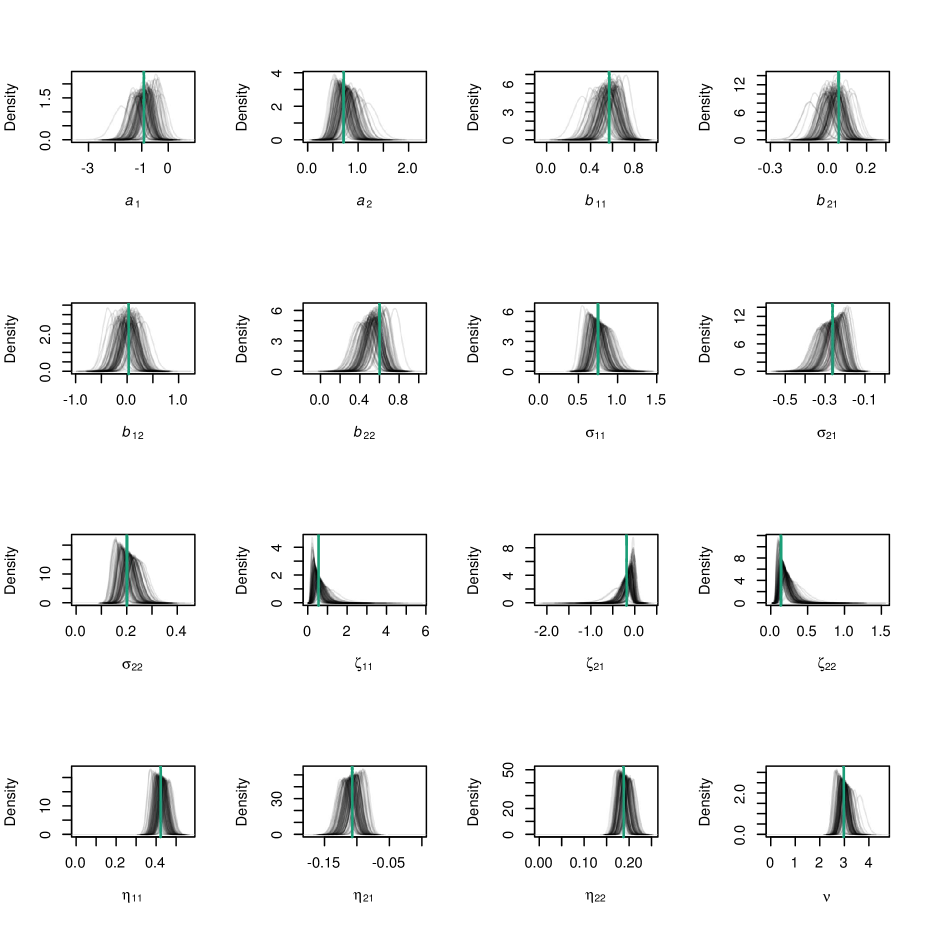
Figure A9: Posterior distributions of parameters estimated from simulated data. Thick green vertical lines: parameter values used to generate simulated data (posterior means from real data). Black lines: kernel density estimates of posterior distributions from 100 simulated data sets, each with the same number of sites, number and spacing of observation times, and numbers of transects at each observation time, as the real data. Number of simulated data sets in which true value was within 95$\%$ HPD interval: 89 ($a_{1}$), 95 ($a_{2}$), 97 ($b_{11}$), 91 ($b_{21}$), 95 ($b_{12}$), 90 ($b_{22}$), 99 ($\sigma_{11}$), 96 ($\sigma_{21}$), 93 ($\sigma_{22}$), 96 ($\zeta_{11}$), 93 ($\zeta_{21}$), 98 ($\zeta_{22}$), 93 ($\eta_{11}$), 93 ($\eta_{21}$), 96 ($\eta_{22}$), 93 ($\nu$).

We ran four Monte Carlo chains in parallel for 5000 iterations each, after a 5000-iteration warmup period. This took approximately two hours on a 64-bit Ubuntu 12.04 system with 4 3.2 GHz Intel Xeon cores and 16 GiB RAM. The potential scale reduction statistic, which takes the value 1 if all chains have converged to a common distribution, was 1.00 to two decimal places for all parameters, consistent with satisfactory convergence (Stan Development Team, 2015b, , pp. 414-415). Effective sample sizes, which measure the size of the sample from the posterior distribution after accounting for autocorrelation in the Monte Carlo chains (Stan Development Team, 2015b, , pp. 417-419), were at least 2839 for all parameters (most were much larger, with first quartile 12430 and median 17490). Inspection of trace plots did not reveal any obvious problems with sampling. In addition, we evaluated the model’s performance in estimating known parameters. We generated 100 simulated data sets with identical structure to the real data, using posterior mean estimates for each parameter. We sampled the $\bm{\alpha}_{i}$, $\bm{\varepsilon}_{i,t}$ and $\mathbf{y}_{i,j,t}$ from distributions defined by Equation A.6, and set the initial true transformed compositions at a given site to the sample means from all years and transects on that site in the real data. The estimates were reasonably close to the true values, and lay within the 95$\%$ HPD intervals in 89-99 out of 100 cases (Figure A9). Thus, while estimating state-space models from ecological time series data can be challenging (Auger-Méthé et al.,, 2015), performance appears adequate in this case, perhaps because we have many replicate transects from which to estimate measurement error and small-scale spatial variability, and most parameters are estimated using data across many sites.

A5.3 Model checking

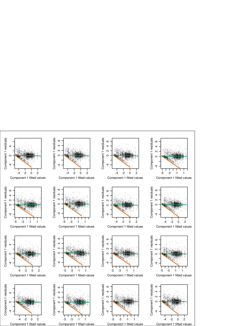
Figure A10: Fitted values against Bayesian residuals for component 1. Each panel is a single randomly-chosen Monte Carlo iteration. Dots represent Bayesian residuals against fitted values for individual transects. The green line is a loess smoother. The orange line is the minimum possible value for component 1 residuals.

We examined plots of Bayesian residuals (Gelman et al.,, 2003, p. 170) against predicted values of the two components of transformed reef composition. For the $k$th Monte Carlo iteration, the Bayesian residual for the $j$th transect on the $i$th site at time $t$ is $\mathbf{y}_{i,j,t}-\mathbf{x}_{i,t}|\bm{\theta}_{k}$, where $\bm{\theta}_{k}$ denotes the estimated parameters in the $k$th iteration. If the model is performing well, there should be no obvious relationship between residuals and fitted values. We checked 16 randomly-chosen iterations, which did not reveal any major cause for concern (Figures A10, A11). However, no residuals for component 1 fell below an obvious diagonal line (Figure A10), which results from the treatment of observed zeros. Given the simple replacement strategy for zeros described in Section A1 and the definition of component 1 of the transformed composition in Equation A.5,

$$y_{1,i,j,t} =\frac{1}{\sqrt{2}}\log\left(\frac{z_{2,i,j,t}}{z_{1,i,j,t}}\right)$$

$$\geq\frac{1}{\sqrt{2}}\log\left(\frac{0.0008}{0.9984}\right) =-5.0216.$$

Thus the Bayesian residual for component 1 is constrained by

$$y_{1,i,j,t}-x_{1,i,t}|\bm{\theta}_{k}\geq-5.0216-x_{1,i,t}|\bm{\theta}_{k},$$

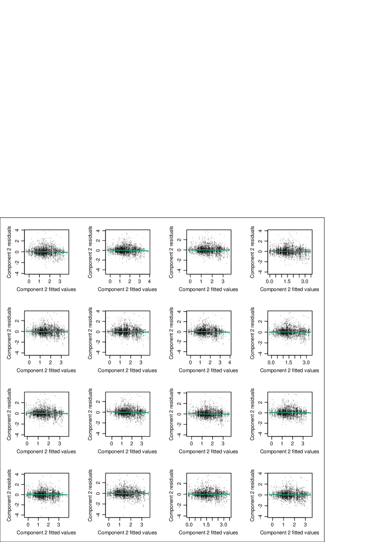
Figure A11: Fitted values against residuals for component 2. Each panel is a single randomly-chosen Monte Carlo iteration. Dots represent Bayesian residuals against fitted values for individual transects. The green line is a loess smoother.

the orange line on Figure A10. Thus the assumption of a multivariate $t$ distribution for individual transect deviations from true values (Equation A.6) cannot hold exactly. It might in future be worth attempting to develop a more mechanistic model of the process generating observed zeros, but we do not attempt this here because the majority of data are unaffected. Although a similar constraint exists on component 2, it did not appear to be important in practice, because there is no obvious diagonal line of residuals on Figure A11.

Inspection of quantile-quantile plots and histograms of estimated skewness and kurtosis for 16 iterations did not indicate any major problems with the assumptions of multivariate normal distributions with zero mean, covariance matrices $\mathbf{Z}$ and $\bm{\Sigma}$ respectively for $\bm{\alpha}$ and $\bm{\varepsilon}$, and a multivariate $t$ distribution with zero location vector, scale matrix $\mathbf{H}$, for Bayesian residuals. Quantile-quantile plots used the natural log of a squared Mahalanobis-like distance/2 against natural log of quantiles of $\chi^{2}(2)$ for multivariate normal distributions, or against natural log of quantiles of $F(2,\nu)$ for multivariate $t$ distributions (modified from Lange et al.,, 1989). We did not transform to asymptotically standard normal deviates because the degrees of freedom for the $t$ distribution were small. We found it helpful to log transform both axes, particularly for the multivariate $t$ distribution, for which some observations may have very large squared Mahalanobis-like distance. We obtained the $p$-values for several tests of multivariate normality of $\bm{\alpha}$ and $\bm{\varepsilon}$: Royston’s $H$ (Royston,, 1982), Henze-Zirkler’s test (Henze and Zirkler,, 1990), and Mardia’s skewness and kurtosis (Mardia,, 1970) using the MVN package in R (Korkmaz et al.,, 2014). There were more small $p$-values than expected (the distribution of $p$-values should be approximately uniform in the interval (0,1) if the data are normal) but that often is the case for very large samples, and does not indicate a major cause for concern.

A6 Long-term behaviour

Iterating Equation A.6 from a fixed initial transformed composition $\mathbf{x}_{i,0}$,

$$\mathbf{x}_{i,t}=\sum_{j=0}^{t-1}\mathbf{B}^{j}\mathbf{a}+\sum_{j=0}^{t-1}\mathbf{B}^{j}\bm{\alpha}_{i}+\mathbf{B}^{t}\mathbf{x}_{0}+\sum_{j=0}^{t-1}\mathbf{B}^{j}\bm{\varepsilon}_{i,t-1-j}$$ (A.7)

If all the eigenvalues of $\mathbf{B}$ lie inside the unit circle in the complex plane, the system will converge to a stationary distribution as $t\rightarrow\infty$ (e.g. Lütkepohl,, 1993, p. 10). If the eigenvalues of $\mathbf{B}$ are complex, they will form a complex conjugate pair $\lambda=re^{\pm i\theta}$ (where $r$ is the magnitude and $\theta$ is the argument), and there will be oscillations with period $2\pi/\theta$, whose amplitudes will change by a factor of $r$ each year (e.g. Otto and Day,, 2007, p. 355).

The first term in Equation A.7 is deterministic, and converges to

$$\bm{\mu}^{*}=(\mathbf{I}_{2}-\mathbf{B})^{-1}\mathbf{a}$$ (A.8)

(e.g. Lütkepohl,, 1993, p. 10), which represents the among-site mean of stationary mean transformed composition. The third term is also deterministic, and converges to $\mathbf{0}$, so that initial conditions are forgotten.

The second term, representing among-site variation, has mean vector $\mathbf{0}$ by definition, and the covariance matrix of its limit is

$$\mathbf{Z}^{*} =\mathrm{V}\left[(\mathbf{I}_{2}-\mathbf{B})^{-1}\bm{\alpha}_{i}\right]$$

$$=(\mathbf{I}_{2}-\mathbf{B})^{-1}\mathrm{V}\left[\bm{\alpha}_{i}\right]\left((\mathbf{I}_{2}-\mathbf{B})^{-1}\right)^{T}$$

$$=(\mathbf{I}_{2}-\mathbf{B})^{-1}\mathbf{Z}\left((\mathbf{I}_{2}-\mathbf{B})^{-1}\right)^{T},$$ (A.9)

since $(\mathbf{I}_{2}-\mathbf{B})^{-1}$ is a constant matrix and $\bm{\alpha}_{i}$ is a random vector. The covariance matrix $\mathbf{Z}^{*}$ represents the among-site variation in stationary mean transformed composition.

The fourth term represents the long-term effects of temporal variability. It has mean vector $\mathbf{0}$ by definition, and it can be shown that it has covariance matrix

$$\bm{\Sigma}^{*}=\mathrm{vec}^{-1}\left((\mathbf{I}_{4}-\mathbf{B}\otimes\mathbf{B})^{-1}\mathrm{vec}\left(\bm{\Sigma}\right)\right)$$ (A.10)

(e.g. Lütkepohl,, 1993, p. 22), where the $\mathrm{vec}$ operator stacks the columns of a matrix, $\mathrm{vec}^{-1}$ unstacks them, and $\otimes$ is the Kronecker product. The covariance matrix $\bm{\Sigma}^{*}$ can be interpreted as the stationary covariance of transformed reef composition, conditional on the value of $\bm{\alpha}_{i}$. Since among-site variation and temporal variation were assumed independent, the unconditional stationary covariance is $\bm{\Sigma}^{*}+\mathbf{Z}^{*}$. Both the conditional and unconditional stationary distributions are multivariate normal, since both $\bm{\varepsilon}_{i,t}$ and $\bm{\alpha}_{i}$ were assumed multivariate normal. Thus the stationary distribution for a randomly-chosen site is the multivariate normal vector

$$\mathbf{x}^{*}\sim\mathcal{N}(\bm{\mu}^{*},\bm{\Sigma}^{*}+\mathbf{Z}^{*}).$$ (A.11)

To find the long-term behaviour for a given site $i$, we condition on the value of $\bm{\alpha}_{i}$. Thus Equation A.8 is replaced by

$$\bm{\mu}_{i}^{*}=(\mathbf{I}_{2}-\mathbf{B})^{-1}(\mathbf{a}+\bm{\alpha}_{i}),$$

and the stationary distribution is

$$\mathbf{x}_{i}^{*}\sim\mathcal{N}(\bm{\mu}_{i}^{*},\bm{\Sigma}^{*}).$$

A7 How important is among-site variability?

From Equation A.11, the covariance matrix $\bm{\Sigma}^{*}+\mathbf{Z}^{*}$ of the stationary distribution for a randomly-chosen site contains contributions from both among- and within-site variability. To quantify the contributions from these two sources, we will use a statistic based on a ratio of generalized variances.

The generalized variance of a multivariate distribution is defined as the determinant of the covariance matrix (Wilks,, 1932; Johnson and Wichern,, 2007, section 3.4). In the specific case of a multivariate normal distribution, the generalized variance may be interpreted in terms of ellipsoids of concentration, defined as follows. Suppose a random vector $\mathbf{W}$ is distributed according to a $p$-dimensional normal distribution with mean vector $\bm{\mu}$ and covariance matrix $\mathbf{V}$. Then for any constant $k\geq 0$, the set $E_{k}=\left\{\mathbf{w}:\left(\mathbf{w}-\bm{\mu}\right)^{T}\mathbf{V}^{-1}\left(\mathbf{w}-\bm{\mu}\right)=k\right\}$ consists of points $\mathbf{w}$ of constant probability density. In $p=2$ dimensions, $E_{k}$ is an ellipse, and may be referred to as a probability density contour. In $p>2$ dimensions $E_{k}$ is known as an ellipsoid of concentration of $\mathbf{V}$ about $\bm{\mu}$ (Kenward,, 1979). Taking $k=1$, the set $E_{1}$ is known as the unit ellipsoid of concentration. The volume within the unit ellipsoid $E_{1}$ may be used as a measure of the dispersion of the distribution, and is equal to $S_{p}\sqrt{\left|\mathbf{V}\right|}$, where $S_{p}$ is the volume of the $p$-dimensional sphere of radius 1.

In the light of the above interpretation, we chose to measure the contribution of within-site variability to total variability using the quantity

$$\rho=\left(\frac{|\bm{\Sigma}^{*}|}{|\bm{\Sigma}^{*}+\mathbf{Z}^{*}|}\right)^{1/2},$$ (A.12)

which is the ratio of volumes of two unit ellipsoids of concentration, the numerator corresponding to the stationary distribution in the absence of among-site variation, and the denominator to the full stationary distribution of transformed reef composition in the region. This ratio is undefined if $\bm{\Sigma}^{*}+\mathbf{Z}^{*}$ is not of full rank, but this does not occur in our application. From Minkowski’s theorem (Mirsky,, 1955, section 13.5) it follows that $|\bm{\Sigma}^{*}|+|\mathbf{Z}^{*}|\leq|\bm{\Sigma}^{*}+\mathbf{Z}^{*}|$, so that $0\leq\rho\leq 1$. However, in general $|\bm{\Sigma}^{*}|+|\mathbf{Z}^{*}|\neq|\bm{\Sigma}^{*}+\mathbf{Z}^{*}|$, so that $\rho$ cannot be simply interpreted as the proportion of total variability explained by within-site variation. Nevertheless, $\rho$ provides an indication of how much of the total variability would remain if all among-site variability was removed. Furthermore, $\rho^{2}$ is analogous to Wilks’ Lambda (Wilks,, 1932; Kenward,, 1979), a likelihood-ratio test statistic often used in multivariate analysis of variance.

A8 Probability of low coral cover

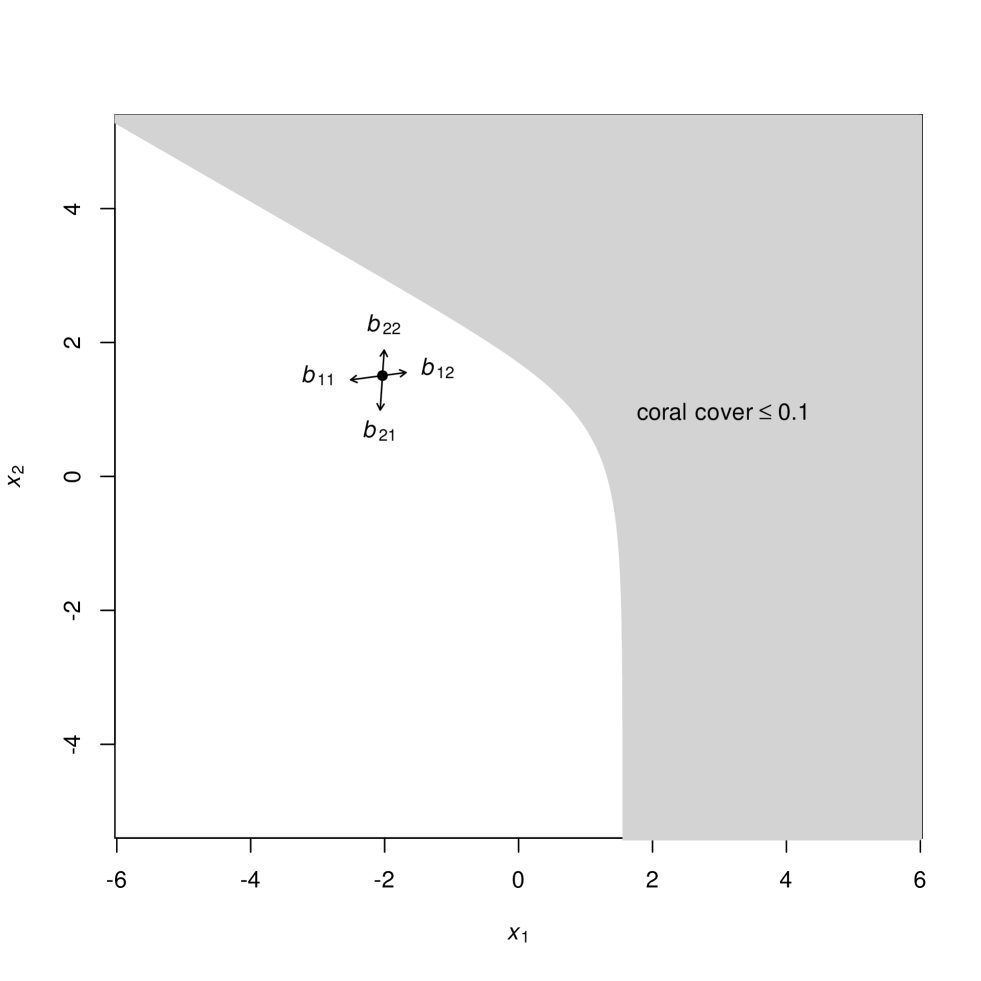
Figure A42: Effects of the elements of $\mathbf{B}$ on the location of the stationary mean $\bm{\mu}^{*}$. Axes: the two components of isometric logratio transformed benthic composition (Equation A.5). Component $x_{1}$ is proportional to the log of the ratio of algae to coral. Component $x_{2}$ is proportional to the log of the ratio of other to the geometric mean of algae and coral. Black dot: point estimate of stationary mean $\bm{\mu}^{*}$, calculated from Equation A.8 using posterior means of $\mathbf{a}$ and $\mathbf{B}$. Arrows: directions of derivatives of $\bm{\mu}^{*}$ with respect to each element of $\mathbf{B}$ (Equation A.16). Shaded region: coral cover $\leq 0.1$.

For a given site $i$, the long-term probability $q_{\kappa,i}$ of coral cover less than or equal to $\kappa$ is the integral of the multivariate normal stationary density for the site over the shaded area in Figure A42 (for $\kappa=0.1$). This can be written as

$$q_{\kappa,i}=1-\int_{-\infty}^{u}P(X_{2}\leq\gamma|X_{1}=x_{1})f_{X_{1}}(x_{1})\,\mathrm{d}x_{1},$$ (A.13)

where, using Equations A.5 and the constraint that the untransformed components of benthic composition must sum to 1,

$$u=\frac{1}{\sqrt{2}}\log\left(\frac{1}{\kappa}-1\right)$$

is the largest value of the first ilr component $x_{1}$ for which it is possible to have coral cover less than or equal to $\kappa$,

$$\gamma=\frac{2}{\sqrt{6}}\log\left(\frac{1-\kappa\left(1+e^{\sqrt{2}x_{1}}\right)}{\kappa\sqrt{e^{\sqrt{2}x_{1}}}}\right)$$

is the value of the second ilr component $x_{2}$ for which coral cover is equal to $\kappa$, given the value of $x_{1}$, $P(X_{2}\leq\gamma|X_{1}=x_{1})$ is the conditional marginal cumulative distribution of $x_{2}$, given the value of $x_{1}$, and $f_{X_{1}}(x_{1})$ is the unconditional marginal density of the first ilr component $x_{1}$.

Since

$$\mathbf{X}=[X_{1},X_{2}]^{T}\sim\mathcal{N}(\mathbf{\mu}_{i}^{*},\bm{\Sigma}_{i}^{*}),$$

the unconditional marginal distribution of $x_{1}$ is

$$\mathcal{N}(\mu_{1,i}^{*},\sqrt{\sigma_{11,i}^{*}}),$$ (A.14)

and the conditional marginal distribution of $x_{2}$ given $x_{1}$ is

$$\mathcal{N}\left(\mu_{2,i}^{*}+\frac{\sigma_{21,i}^{*}}{\sigma_{11,i}^{*}}(x_{1}-\mu_{i,1}^{*}),\sigma_{22,i}^{*}-\frac{(\sigma_{21,i}^{*})^{2}}{\sigma_{11,i}^{*}}\right)$$ (A.15)

(Gelman et al.,, 2003, p. 579). Then the integral in Equation A.13 can be approximated numerically using the integrate() function in R (R Core Team,, 2015), which is based on routines in Piessens et al., (1983). The same approach can be used for $q_{\kappa}$ for a randomly-chosen site, replacing the elements of $\bm{\mu}_{i}^{*}$ and $\bm{\Sigma}_{i}^{*}$ in Equations A.14 and A.15 with the corresponding elements of $\bm{\mu}^{*}$ and $\bm{\Sigma}^{*}$.

A9 Spline correlograms for spatial pattern in probability of low coral cover

We calculated a spline correlogram (Bjørnstad and Falck,, 2001) for each set of $q_{0.1,i}$ in the 20000 Monte Carlo iterations, using the spline.correlog() function in the R package ncf version 1.15. We constructed a 95$\%$ highest-density envelope (Hyndman,, 1996) for the resulting set of correlograms using the R package hdrcde version 3.1.

A10 What is the most effective way to reduce the probability of low coral cover?

For a given threshold $\kappa$, we can calculate (by numerical integration) the probability $q_{\kappa}=P(\text{coral cover}\leq\kappa)$, for a composition drawn from the stationary distribution on a site chosen at random from the region. The probability $q_{\kappa}$ is a function of 12 parameters: all four elements of $\mathbf{B}$; both elements of $\mathbf{a}$; elements $\sigma_{11}$, $\sigma_{21}$ and $\sigma_{22}$ of $\bm{\Sigma}$; and elements $\zeta_{11}$, $\zeta_{21}$ and $\zeta_{22}$ of $\mathbf{Z}$. Note that because $\bm{\Sigma}$ and $\mathbf{Z}$ are covariance matrices, they must be symmetric, and so $\sigma_{12}$ and $\zeta_{12}$ are not free parameters. These 12 parameters can be thought of as the coordinates of a point in $\mathbb{R}^{12}$. The steepest reduction in $q_{\kappa}$ as we move through $\mathbb{R}^{12}$ is achieved by moving in the direction of $-\bm{\nabla}q_{\kappa}$, where $\bm{\nabla}q_{\kappa}$ is the gradient vector $[\partial q_{\kappa}/\partial b_{11},\ldots,\partial q_{\kappa}/\partial\zeta_{22}]^{T}$ (Riley et al.,, 2002, p. 355).

To understand the effects of each parameter, note that the probability $q_{\kappa}$ depends on these parameters only through $\bm{\mu}^{*}$, $\bm{\Sigma}^{*}$ and $\mathbf{Z}^{*}$. Thus, for any parameter matrix $\bm{\Theta}$, using the chain rule for matrix derivatives,

$$Dq_{\kappa}(\bm{\Theta})=Dq_{\kappa}(\bm{\mu}^{*})D\bm{\mu}^{*}(\bm{\Theta})+Dq_{\kappa}(\bm{\Sigma}^{*})D\bm{\Sigma}^{*}(\bm{\Theta})+Dq_{\kappa}(\mathbf{Z}^{*})D\mathbf{Z}^{*}(\bm{\Theta}),$$

where $D\mathbf{E}(\mathbf{X})$ denotes the matrix derivative of $\mathbf{E}$ with respect to $\mathbf{X}$ (Magnus and Neudecker,, 2007, p. 108). This allows us to break up the effects of a parameter into its effects via the stationary mean and stationary within- and among-site covariances. In each term, the first factor ($Dq_{\kappa}(\bm{\mu}^{*})$, $Dq_{\kappa}(\bm{\Sigma}^{*})$ or $D\bm{\Sigma}^{*}(\bm{\Theta})$) can only be found numerically. The non-zero second factors are

$$D\bm{\mu}^{*}(\mathbf{B}) =(\mathbf{a}^{T}\otimes\mathbf{I}_{2})\left[\left((\mathbf{I}_{2}-\mathbf{B})^{-1}\right)^{T}\otimes(\mathbf{I}_{2}-\mathbf{B})^{-1}\right],$$ (A.16)

$$D\bm{\Sigma}^{*}(\mathbf{B}) =\mathbf{F}\left[(\mathrm{vec}\bm{\Sigma})^{T}\otimes\mathbf{I}_{4}\right]\left[\left((\mathbf{I}_{4}-\mathbf{B}\otimes\mathbf{B})^{-1}\right)^{T}\otimes(\mathbf{I}_{4}-\mathbf{B}\otimes\mathbf{B})^{-1}\right]$$

$$(\mathbf{I}_{2}\otimes\mathbf{K}_{4}\otimes\mathbf{I}_{2})(\mathbf{I}_{4}\otimes\mathrm{vec}\mathbf{B}+\mathrm{vec}\mathbf{B}\otimes\mathbf{I}_{4}),$$

$$D\mathbf{Z}^{*}(\mathbf{B}) =\mathbf{F}\left[(\mathrm{vec}\mathbf{Z})^{T}\otimes\mathbf{I}_{4}\right](\mathbf{I}_{2}\otimes\mathbf{K}_{4}\otimes\mathbf{I}_{2})\left[\mathbf{I}_{4}\otimes\mathrm{vec}(\mathbf{I}_{2}-\mathbf{B})^{-1}+\mathrm{vec}(\mathbf{I}_{2}-\mathbf{B})^{-1}\otimes\mathbf{I}_{4}\right]$$

$$\left[\left((\mathbf{I}_{2}-\mathbf{B})^{-1}\right)^{T}\otimes(\mathbf{I}_{2}-\mathbf{B})^{-1}\right],$$

$$D\bm{\mu}^{*}(\mathbf{a}) =(\mathbf{I}_{2}-\mathbf{B})^{-1},$$

$$D\bm{\Sigma}^{*}(\bm{\Sigma}) =\mathbf{F}(\mathbf{I}_{4}-\mathbf{B}\otimes\mathbf{B})^{-1}\mathbf{G},$$

$$D\mathbf{Z}^{*}(\mathbf{Z}) =\mathbf{F}\left[(\mathbf{I}_{2}-\mathbf{B})^{-1}\otimes(\mathbf{I}_{2}-\mathbf{B})^{-1}\right]\mathbf{G},$$

where $\mathbf{K}_{4}$ is the $4\times 4$ commutation matrix (Magnus and Neudecker,, 2007, p. 54),

$$\mathbf{F}=\begin{bmatrix}1&0&0&0\\ 0&1&0&0\\ 0&0&0&1\end{bmatrix},$$

and

$$\mathbf{G}=\begin{bmatrix}1&0&0\\ 0&1&0\\ 0&1&0\\ 0&0&1\end{bmatrix}.$$

A11 How informative is a snapshot about long-term site properties?

Denote the true state of a randomly-chosen site at a given time by $\mathbf{x}$, and the corresponding stationary mean for that site by $\bm{\mu}^{*}$. Under the model of Equation A.6, $\bm{\mu}^{*}$ has covariance matrix $\mathbf{Z}^{*}$ (Equation A.9). Write the true state as $\mathbf{x}=\bm{\mu}^{*}+\bm{\Delta}$, where $\bm{\Delta}$ is the deviation from the stationary mean, which has covariance matrix $\bm{\Sigma}^{*}$ (Equation A.10). The correlation $\rho_{k}$ between the $k$th component $x_{k}$ of $\mathbf{x}$ and the corresponding component $\mu_{k}^{*}$ of $\bm{\mu}^{*}$ is an obvious way to measure how informative the snapshot will be for this component. This is

$$\rho_{k} =\frac{\text{cov}(\mu^{*}_{k}+\Delta_{k},\mu^{*}_{k})}{\sqrt{V[\mu^{*}_{k}+\Delta_{k}]V[\mu^{*}_{k}]}}$$

$$=\frac{V[\mu^{*}_{k}]+\text{cov}(\mu^{*}_{k},\Delta_{k})}{\sqrt{V[\mu^{*}_{k}+\Delta_{k}]V[\mu^{*}_{k}]}}$$

$$=\frac{V[\mu^{*}_{k}]}{\sqrt{(V[\mu^{*}_{k}]+V[\Delta_{k}])V[\mu^{*}_{k}]}}\quad\text{(because $\bm{\alpha}$ and $\bm{\varepsilon}$ assumed independent)}$$

$$=\left(\frac{\zeta^{*}_{kk}}{\zeta^{*}_{kk}+\sigma^{*}_{kk}}\right)^{1/2},$$

where $\zeta^{*}_{kk}$ is the $k$th diagonal element of $\mathbf{Z}^{*}$, and $\sigma^{*}_{kk}$ is the $k$th diagonal element of $\bm{\Sigma}^{*}$. If $\rho_{k}$ is far from zero, a snapshot will be a reliable guide to the long-term value of the $k$th component of transformed reef composition. On the other hand, if $\rho_{k}$ is close to zero, a snapshot will be unreliable. Thus $\rho_{k}$ measures the extent to which conservation and management decisions could be based on observations at a single time point. We computed both $\rho_{1}$ which tells us how much we could learn about the log of the ratio of algae to coral and $\rho_{2}$, which tells us how much we could learn about the log of the ratio of other to the geometric mean of coral and algae.

A12 Dynamics

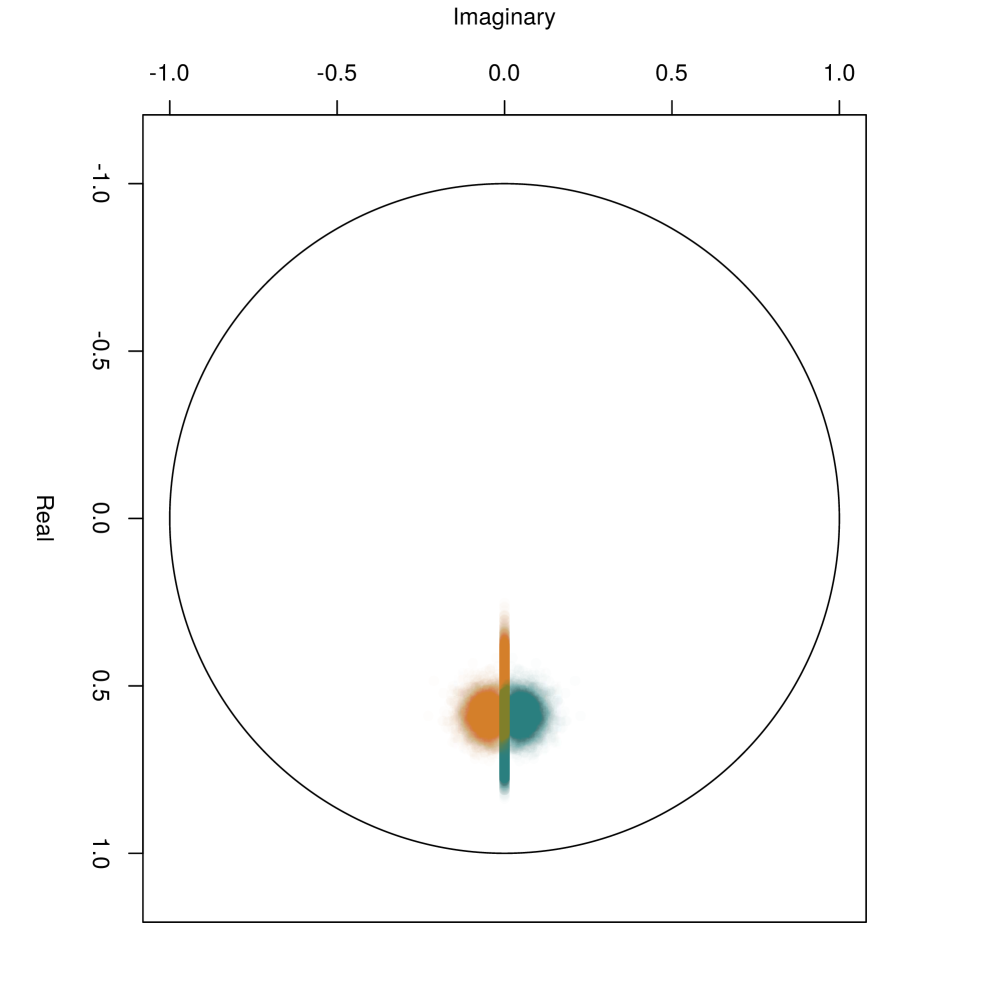
Figure A43: Distribution of the two eigenvalues of $\mathbf{B}$ in the complex plane. Each Monte Carlo sample gives a pair of eigenvalues, represented by two points: $\lambda_{1}$ (green), posterior mean magnitude 0.64, $95\%$ HPD interval $[0.53,0.75]$; $\lambda_{2}$ (orange), posterior mean magnitude 0.53, $95\%$ HPD interval $[0.41,0.66]$)

Consistent with the patterns suggesting negative feedbacks that will tend to maintain fairly stable reef composition, every set of sampled parameters led to a stationary distribution (Figure A43: all sampled eigenvalues of $\mathbf{B}$ fell inside the unit circle in the complex plane, with maximum magnitude 0.84). In $27\%$ of iterations, there was evidence for oscillations on the approach to the stationary distribution, because the eigenvalues were complex. In such cases, the oscillations had a long period (posterior mean 113 years, $95\%$ HPD interval $[21,284]$ years), but their amplitude more than halved within three years because the magnitudes of the eigenvalues involved were small (original posterior mean magnitude of complex eigenvalues 0.59, $95\%$ credible interval $[0.51,0.67]$, cubed posterior mean magnitude 0.21, $95\%$ HPD interval $[0.13,0.30]$). The distribution of eigenvalues was very different from that of the Great Barrier Reef (Cooper et al.,, 2015, Appendix A.10), where the largest eigenvalue lay close to the point beyond which the stationary distribution would not exist (bootstrap mean magnitude 0.95), and there was no evidence for oscillations (no bootstrap replicates had complex eigenvalues). However, a different estimation method was used in Cooper et al., (2015), so the eigenvalues may not be directly comparable.

A13 Probability of low coral cover: signs of derivatives

Here, we explain the signs of the derivatives of the probability of low coral cover with respect to each parameter. We concentrate on coral cover threshold 0.1. The overall stationary mean $\bm{\mu}^{*}$ lies in the region where coral cover is greater than 0.1 for all iterations (Figure A42, black circle, shows a point estimate for $\bm{\mu}^{*}$, based on the stationary means of $\mathbf{a}$ and $\mathbf{B}$). The shaded region of Figure A42 has coral cover $\leq 0.1$. Because of the shape of the boundary of the shaded region, either increasing $\mu_{1}^{*}$ (increasing the ratio of algae to coral) or increasing $\mu_{2}^{*}$ (increasing the ratio of other to the geometric mean of coral and algae) will move the stationary mean closer to this region. Also, since the stationary mean lies outside the region of interest, increasing the variability in the stationary distribution by increasing the elements of $\bm{\Sigma}^{*}$ or $\mathbf{Z}^{*}$ will increase the probability of falling in the region of interest. Hence the derivatives of $q_{0.1}$ with respect to $\bm{\mu}^{*}$, $\bm{\Sigma}^{*}$, $\mathbf{Z}^{*}$ contain only positive elements.

It is then intuitively obvious that the derivatives of $q_{0.1}$ with respect to $\bm{\Sigma}$ and $\mathbf{Z}$ will contain only positive elements. Increasing the amount of year-to-year temporal variability or among-site variability will increase the variability in the stationary distribution, and hence the long-term probability of coral cover less than or equal to 0.1.

The signs of the derivatives of $q_{0.1}$ with respect to $\mathbf{a}$ are also easy to understand. The components $a_{1}$, $a_{2}$ represent the rates of increase of $x_{1}$ and $x_{2}$ respectively, so we would expect that increasing either of them will increase the corresponding component of the stationary mean. Thus the derivatives of $\bm{\mu}^{*}$ with respect to $\mathbf{a}$ will be positive, and from Figure A42, increasing either component of $\bm{\mu}^{*}$ will increase the probability of coral cover $\leq 0.1$.

The derivatives of $q_{0.1}$ with respect to $\mathbf{B}$ are a little harder to understand. They are (predominantly) negative with respect to $b_{11}$ and $b_{21}$, but positive with respect to $b_{12}$ and $b_{22}$. Since $\mathbf{B}$ affects both the stationary mean (Equation A.8) and the stationary covariance, which is the sum of $\bm{\Sigma}^{*}$ (Equation A.10) and $\mathbf{Z}^{*}$ (Equation A.9), all of these effects could be important. However, in 93$\%$ of iterations,

$$|Dq_{0.1}(\bm{\mu}*)D\bm{\mu}^{*}(\mathbf{B})|\succ|Dq_{0.1}(\bm{\Sigma}^{*})D\bm{\Sigma}^{*}(\mathbf{B})+Dq_{0.1}(\mathbf{Z}^{*})D\mathbf{Z}^{*}(\mathbf{B})|,$$

where $\succ$ is an elementwise inequality, and $|\mathbf{D}|$ indicates the elementwise magnitude, such that for two matrices $\mathbf{D}$ and $\mathbf{E}$ with the same dimensions, $|\mathbf{D}|\succ|\mathbf{E}|$ if and only if the magnitude of every $d_{ij}$ is greater than the magnitude of the corresponding $e_{ij}$. In other words, in almost all iterations, the sign of the effect of $\mathbf{B}$ on $q_{0.1}$ via $\bm{\mu}^{*}$ determines the sign of the overall effect of $\mathbf{B}$ on $q_{0.1}$. We therefore concentrate on understanding how $\mathbf{B}$ affects $\bm{\mu}^{*}$.

To understand the signs of the effects of $b_{11}$ and $b_{22}$ on $\bm{\mu}^{*}$, consider the one-dimensional deterministic analogue

$$x_{t+1}=a+bx_{t}.$$

Iterating this gives

$$x_{t}=a\left(1+b+b^{2}+\ldots+b^{t-1}\right)+b^{t}x_{0}.$$

For $0<b<1$, the term $b^{t}x_{0}\rightarrow\ 0$ as $t\rightarrow\infty$. Then the derivative of $x_{\infty}$ with respect to $b$ has the same sign as $a$. In our system, $a_{1}<0$ and $a_{2}>0$, so we expect the signs of derivatives of $\bm{\mu}^{*}$ with respect to $b_{11}$ to be negative, and the signs of derivatives of $\bm{\mu}^{*}$ with respect to $b_{22}$ to be positive.

To understand the signs of the effects of $b_{12}$ and $b_{21}$ on $\bm{\mu}^{*}$, recall that $b_{12}$ is the effect of component 2 (which typically takes positive values) on component 1, and $b_{21}$ is the effect of component 1 (which typically takes negative values) on component 2. If, as in our system, $b_{12}$ and $b_{21}$ are both positive, and the system is linear, we would expect that the signs of their effects on $\bm{\mu}^{*}$ will be the same as the signs of components 2 and 1 respectively.

Then, by the graphical argument above (Figure A42), we expect the signs of the derivatives of $q_{0.1}$ with respect to $b_{11}$, $b_{21}$, $b_{12}$ and $b_{22}$ to be $-$,$-$,$+$,$+$ respectively.

A14 Probability of low coral cover: rank order and other thresholds

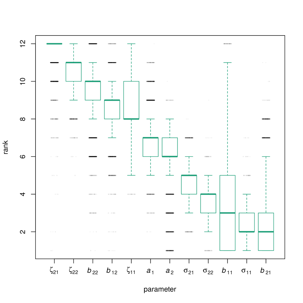
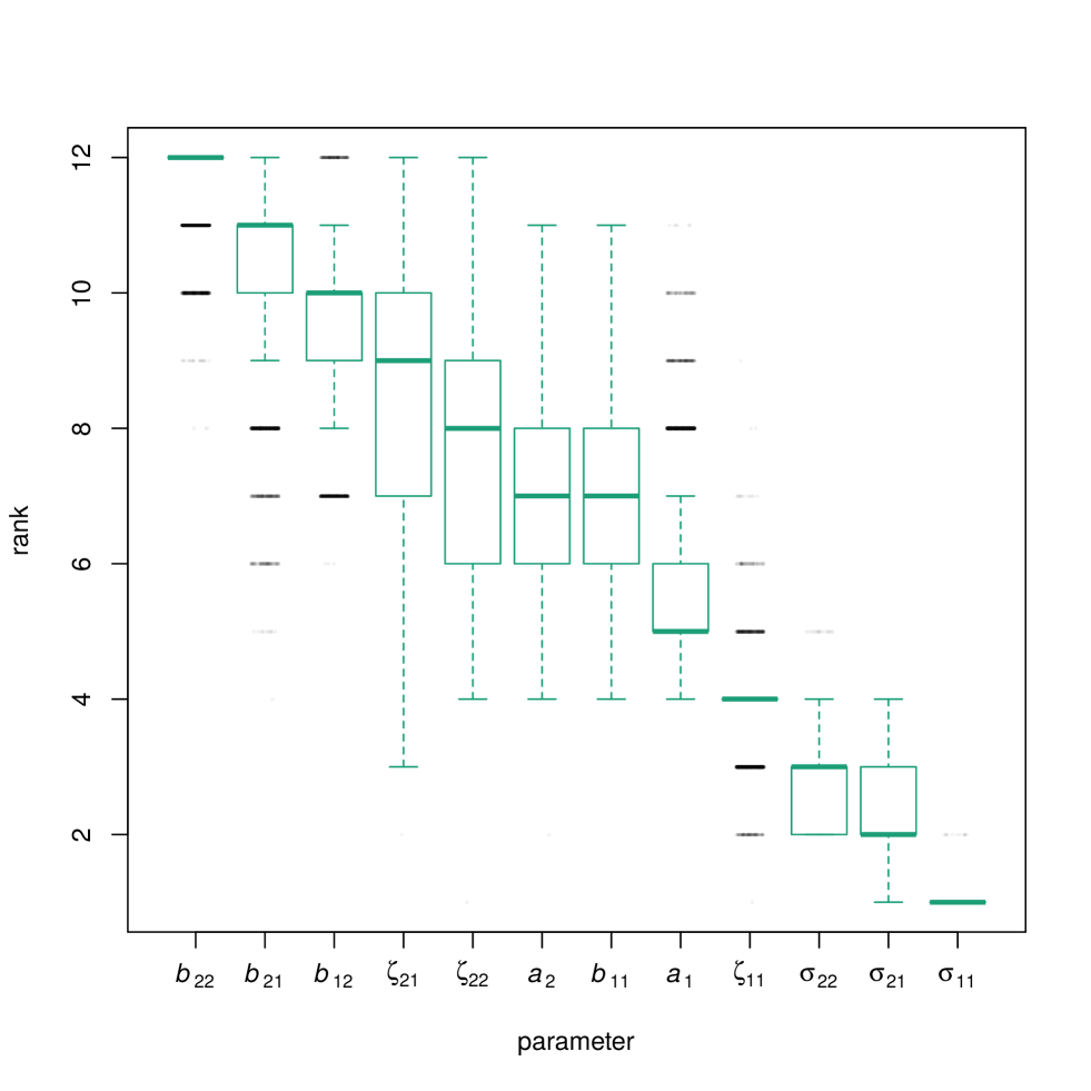
Figure A46: Elements of the gradient vector of partial derivatives of the long-term probability of coral cover less than or equal to 0.05 with respect to elements of the $\mathbf{B}$ matrix, the $\mathbf{a}$ vector, the covariance matrix of random temporal variation $\bm{\Sigma}$, and the covariance matrix of among-site variability $\mathbf{Z}$. For each parameter, the dot is the posterior mean and the bar is a 95$\%$ HPD interval. For the covariance matrices, the elements $\sigma_{12}$ and $\zeta_{12}$ are not shown, because they are constrained to be equal to $\sigma_{21}$ and $\zeta_{21}$ respectively.

Figure A47: Ranks of partial derivatives of the long-term probability of coral cover less than or equal to 0.05 with respect to elements of the $\mathbf{B}$ matrix, the $\mathbf{a}$ vector, the covariance matrix of random temporal variation $\bm{\Sigma}$, and the covariance matrix of among-site variability $\mathbf{Z}$. Parameters are ranked in descending order of median rank (higher ranks indicate larger magnitudes of partial derivative). Outliers are indicated as jittered black dots. For the covariance matrices, the elements $\sigma_{12}$ and $\zeta_{12}$ are not shown, because they are constrained to be equal to $\sigma_{21}$ and $\zeta_{21}$ respectively.

For threshold 0.05, the signs of the effects of $b_{11}$ and $b_{21}$ were not clearly negative. The four most important parameters were (in descending order: Figure A47) $\zeta_{21}$, $\zeta_{22}$, $b_{22}$ and $b_{12}$ (the same four as for threshold 0.1, but in a different order). For threshold 0.2, the signs were as for threshold 0.1, but the four most important parameters were (in descending order) $b_{22}$, $b_{21}$, $b_{12}$ and $\zeta_{21}$ (with $\zeta_{22}$ now in fifth place: Figure A49). Thus, while the details depend to some extent on the threshold, the overall conclusion that both internal dynamics and among-site variability are the most important factors affecting the probability of low coral cover is robust.

The effects of within-site temporal variability on the probability of low coral cover were always relatively unimportant (threshold 0.1, Figure A45, three of the last four positions in the ranked list; threshold 0.05, Figure A47, three of the last five positions; threshold 0.20, Figure A49, last three positions).

Table A1: Reef features. For each named reef, surveys were done at either one site, or at two sites $20\text{\,}\mathrm{m}100\text{\,}\mathrm{m}$ apart. Fished reefs include community management areas with reduced harvesting intensity, and unfished reefs include those recently designated as reserves. Mean coral cover is the arithmetic mean of observed coral cover over all transects and time points.

Reef	Sites	Location	Time points	Time range	Reef type	Management	Mean coral cover (site 1, site 2)
Bongoyo	2	6.67 S, 39.26 E	3	1995-2012	patch	fished	54.7, 52.1
Changale	1	5.30 S, 39.10 E	3	1995-2010	patch	fished	39.4
Changuu	1	6.12 S, 39.12 E	3	1997-2012	patch	fished	46.8
Chapwani	1	6.07 S, 39.11 E	3	1997-2012	patch	fished	52.5
Chumbe	2	6.28 S, 39.17 E	3	1997-2012	patch	unfished	70.1, 74.1
Diani	2	4.37 S, 39.58 E	19	1992-2013	fringing	fished	32.0, 17.5
Funguni	1	5.27 S, 39.13 E	3	1995-2010	patch	fished	13.7
Kanamai	2	3.93 S, 39.78 E	19	1991-2013	fringing	fished	33.0, 32.3
Kisite	2	4.71 S, 39.37 E	8	1994-2012	patch	unfished	33.9, 46.4
Makome	1	5.28 S, 39.11 E	3	1995-2010	patch	fished	32.1
Malindi	2	3.26 S, 40.15 E	20	1991-2013	fringing	unfished	27.9
Mbudya	2	6.66 S, 39.25 E	3	1995-2012	patch	fished	53.5, 68.0
Mombasa	2	3.99 S, 39.75 E	20	1991-2013	fringing	unfished	37.27, 29.2
Mradi	1	3.94 S, 39.78 E	2	2010-2011	fringing	fished	48.4
Nyali	2	4.05 S, 39.71 E	2	2006-2009	fringing	fished	28.1, 29.1
Ras Iwatine	1	4.02 S, 39.73 E	18	1993-2013	fringing	fished	10.8
Taa	1	3.99 S, 39.77 E	3	1995-2010	patch	fished	20.7
Tiwi Inside	1	4.26 S, 39.61 E	2	2008-2011	fringing	fished	36.0
Vipingo	2	3.48 S, 39.95 E	18 (site 1), 19 (site 2)	1991-2013	fringing	fished	28.0, 28.2
Watamu	1	3.37 S, 40.01 E	20	1991-2013	fringing	unfished	23.2

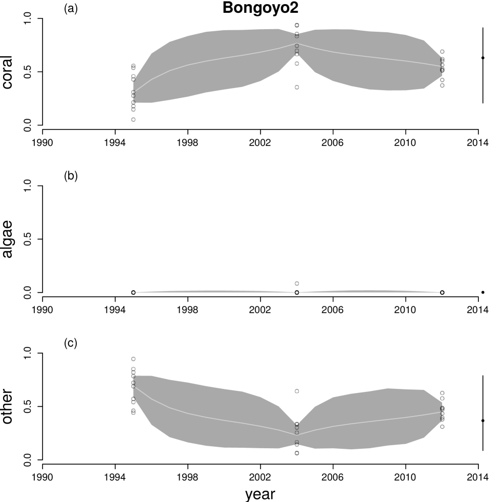
Figure A13: Time series for cover of hard corals (a), macroalgae (b) and other (c) at Bongoyo2. See Figure A12 legend for explanation.

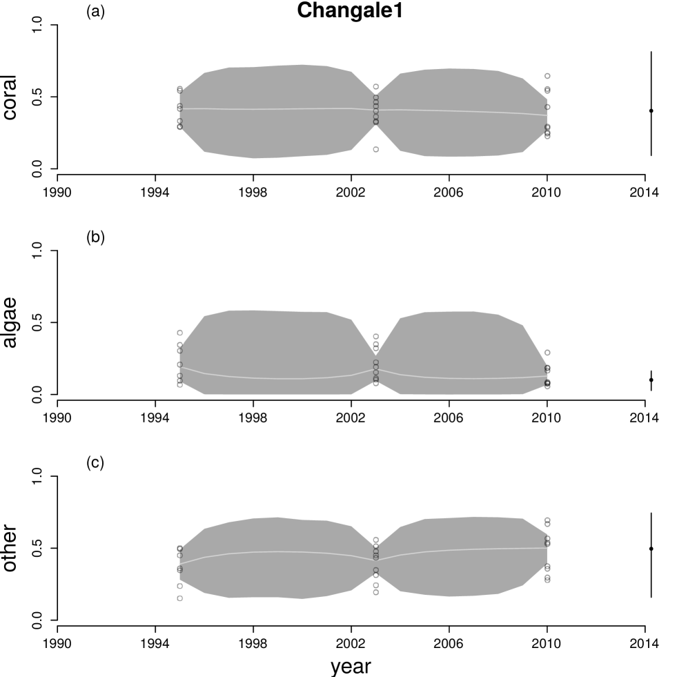
Figure A14: Time series for cover of hard corals (a), macroalgae (b) and other (c) at Changale1. See Figure A12 legend for explanation.

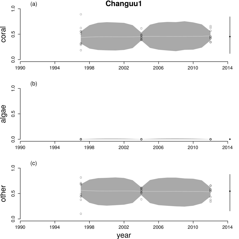
Figure A15: Time series for cover of hard corals (a), macroalgae (b) and other (c) at Changuu1. See Figure A12 legend for explanation.

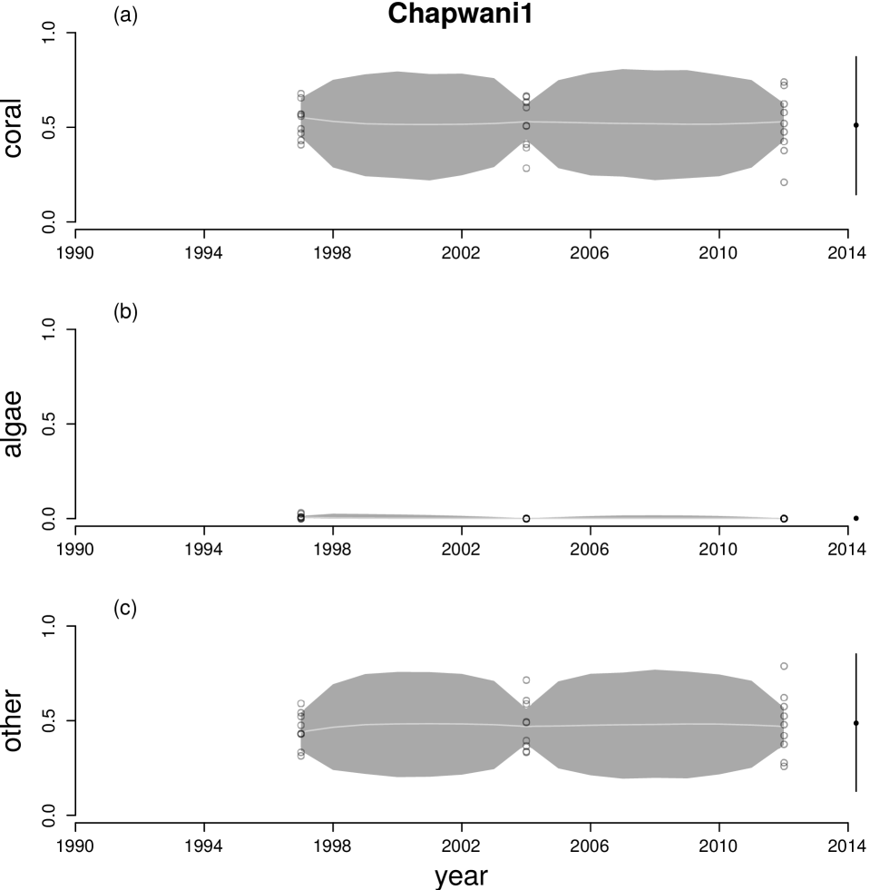
Figure A16: Time series for cover of hard corals (a), macroalgae (b) and other (c) at Chapwani1. See Figure A12 legend for explanation.

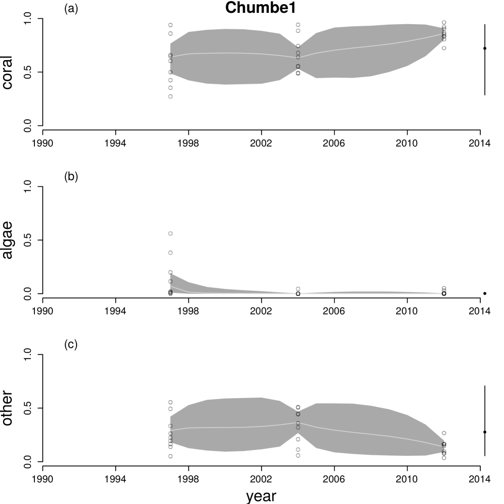
Figure A17: Time series for cover of hard corals (a), macroalgae (b) and other (c) at Chumbe1. See Figure A12 legend for explanation.

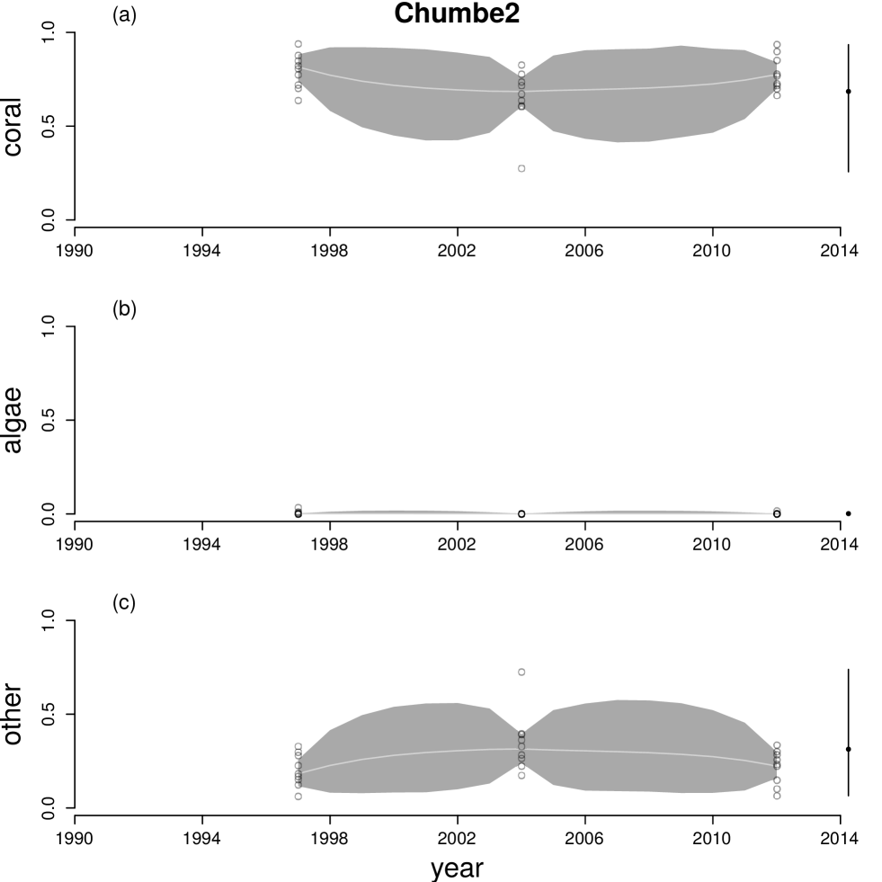
Figure A18: Time series for cover of hard corals (a), macroalgae (b) and other (c) at Chumbe2. See Figure A12 legend for explanation.

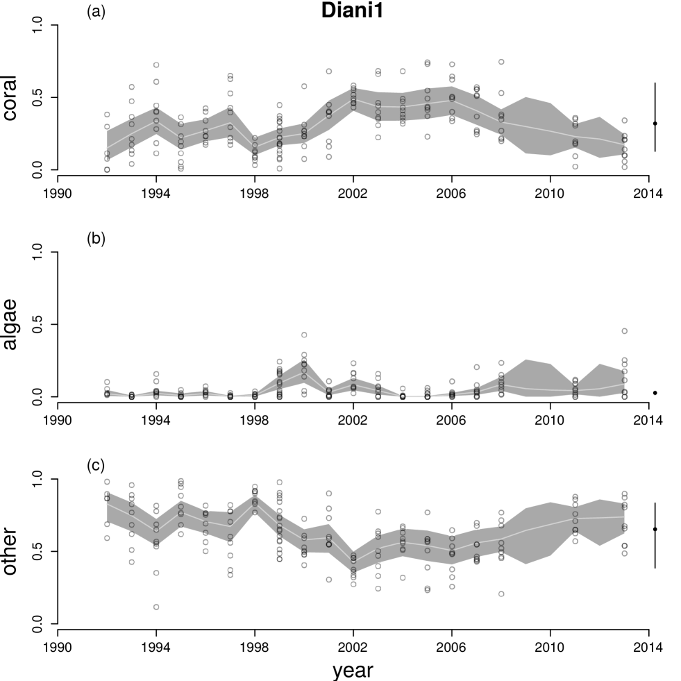
Figure A19: Time series for cover of hard corals (a), macroalgae (b) and other (c) at Diani1. See Figure A12 legend for explanation.

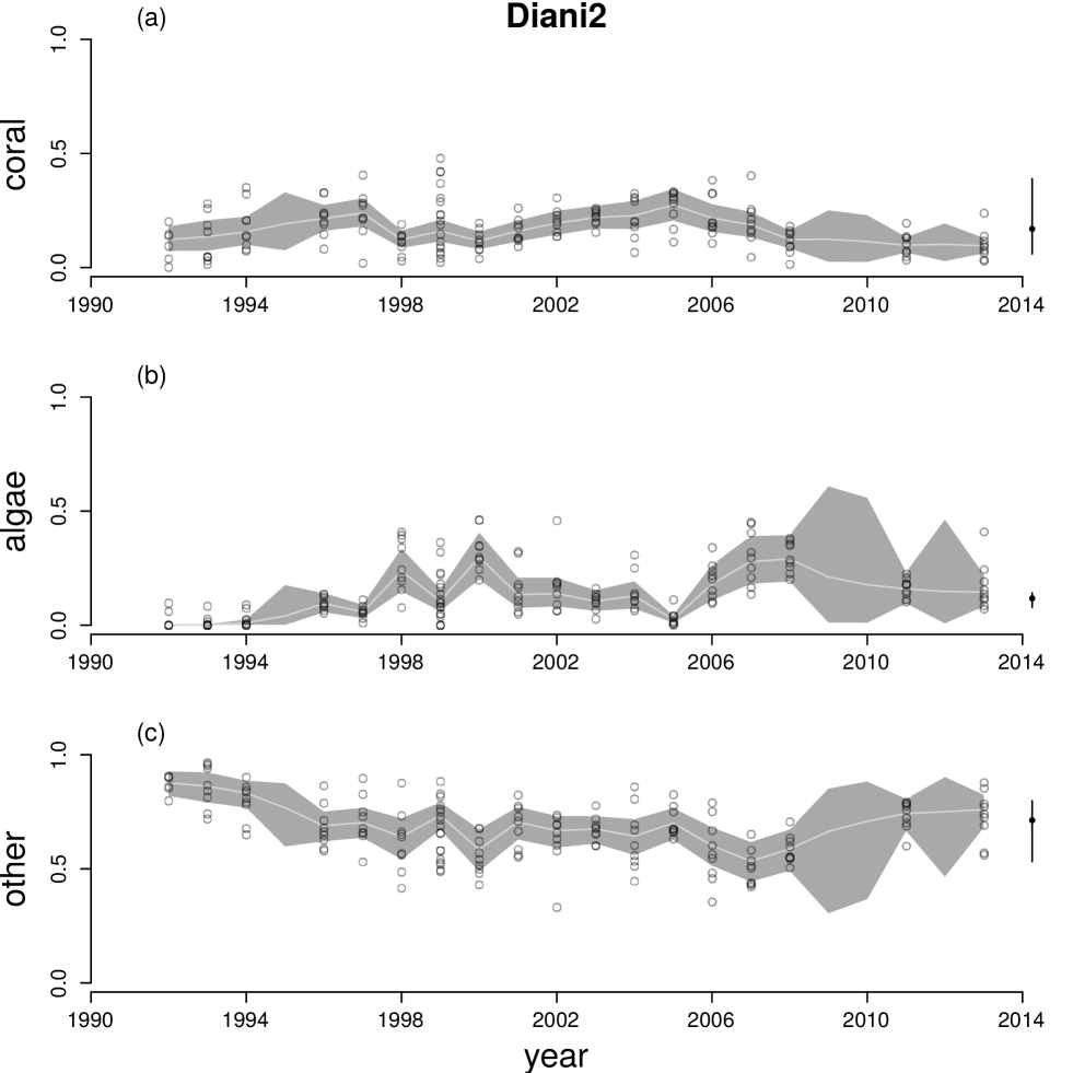
Figure A20: Time series for cover of hard corals (a), macroalgae (b) and other (c) at Diani2. See Figure A12 legend for explanation.

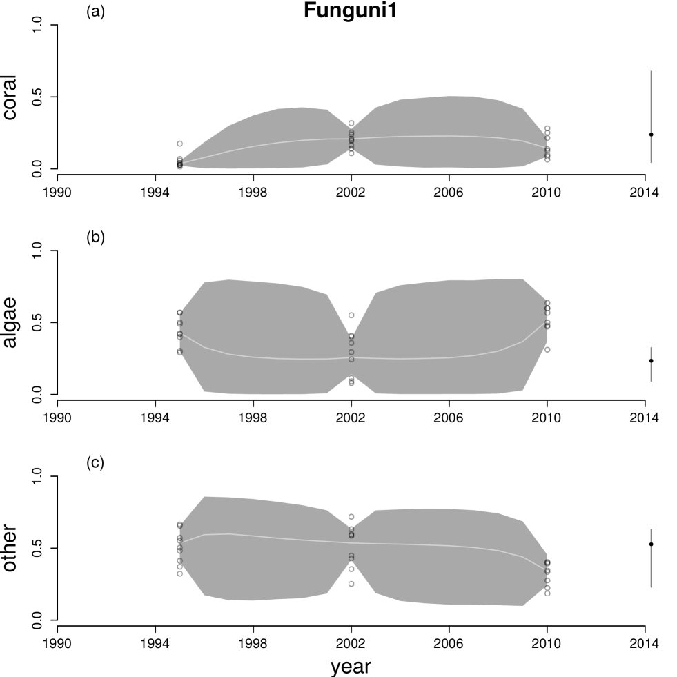
Figure A21: Time series for cover of hard corals (a), macroalgae (b) and other (c) at Funguni1. See Figure A12 legend for explanation.

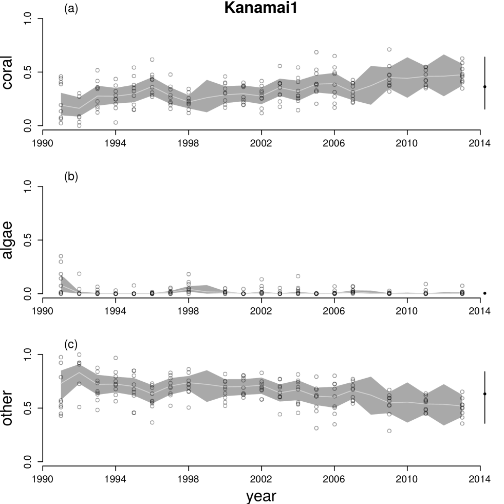
Figure A22: Time series for cover of hard corals (a), macroalgae (b) and other (c) at Kanamai1. See Figure A12 legend for explanation.

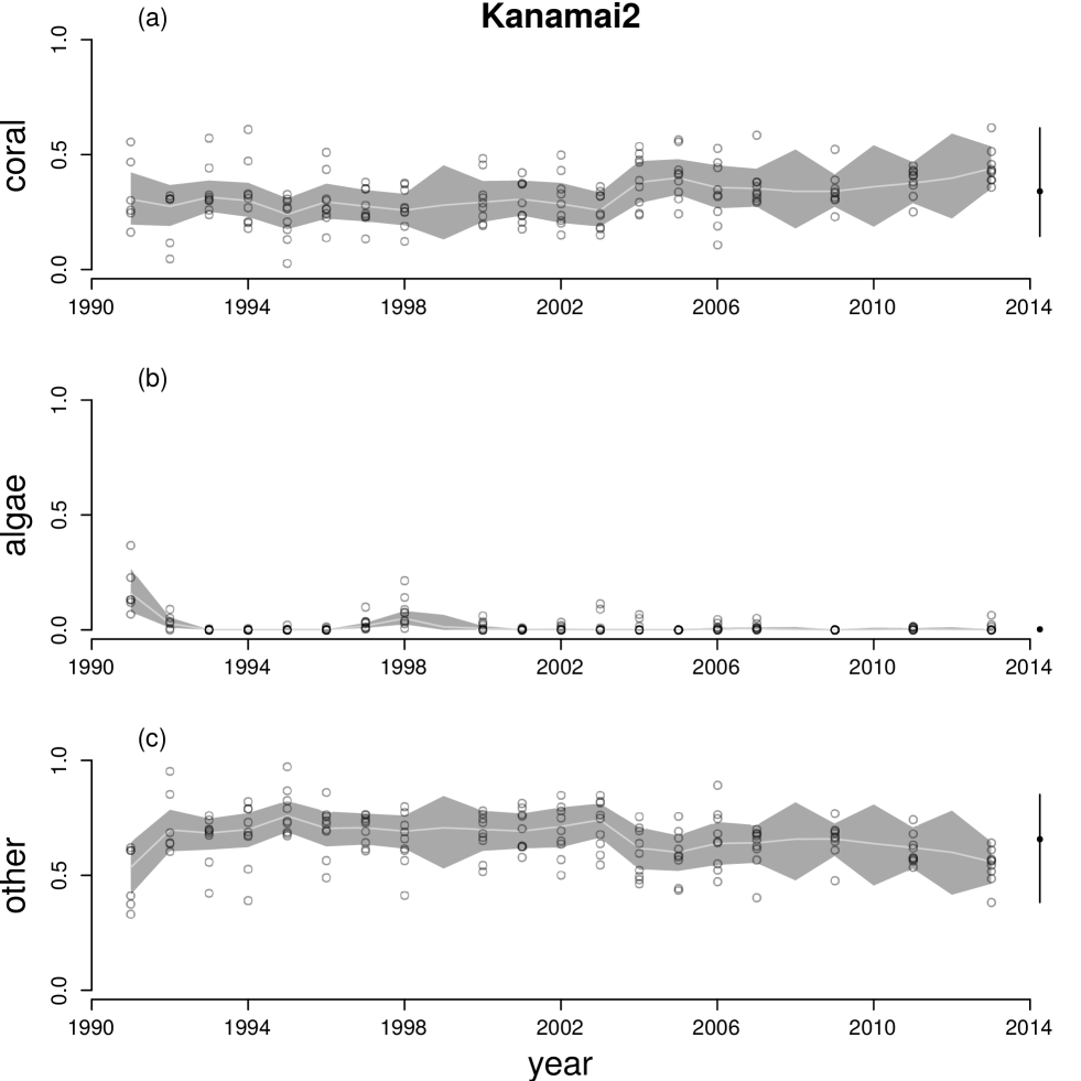
Figure A23: Time series for cover of hard corals (a), macroalgae (b) and other (c) at Kanamai2. See Figure A12 legend for explanation.

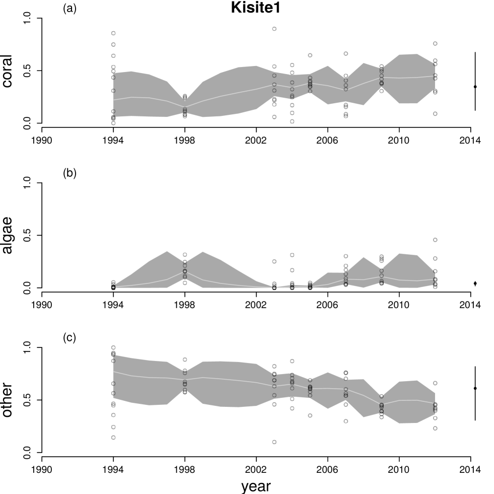
Figure A24: Time series for cover of hard corals (a), macroalgae (b) and other (c) at Kisite1. See Figure A12 legend for explanation.

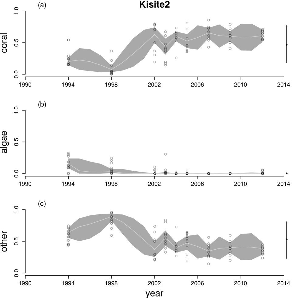
Figure A25: Time series for cover of hard corals (a), macroalgae (b) and other (c) at Kisite2. See Figure A12 legend for explanation.

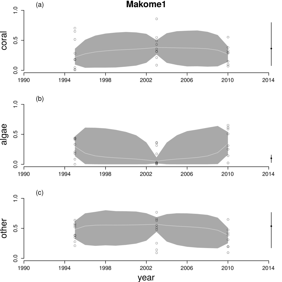
Figure A26: Time series for cover of hard corals (a), macroalgae (b) and other (c) at Makome1. See Figure A12 legend for explanation.

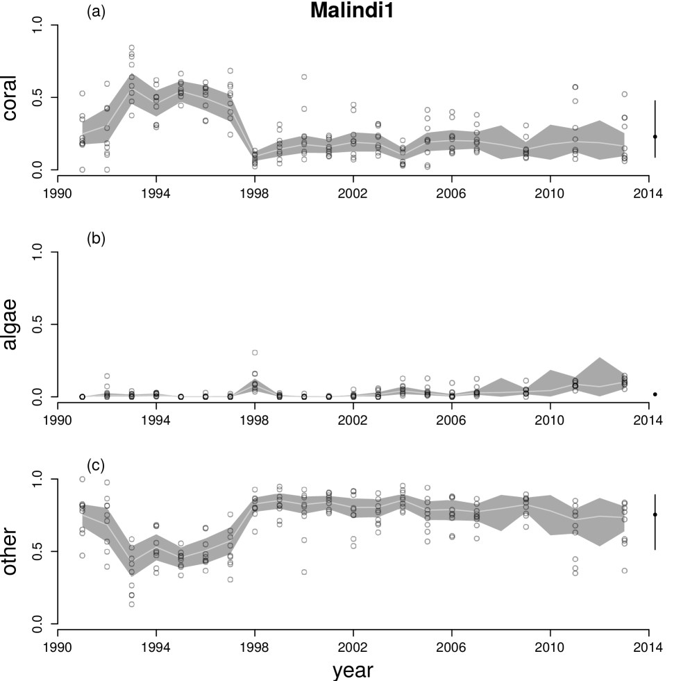
Figure A27: Time series for cover of hard corals (a), macroalgae (b) and other (c) at Malindi1. See Figure A12 legend for explanation.

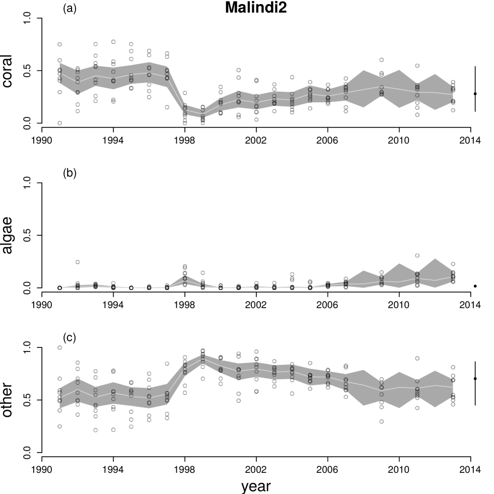
Figure A28: Time series for cover of hard corals (a), macroalgae (b) and other (c) at Malindi2. See Figure A12 legend for explanation.

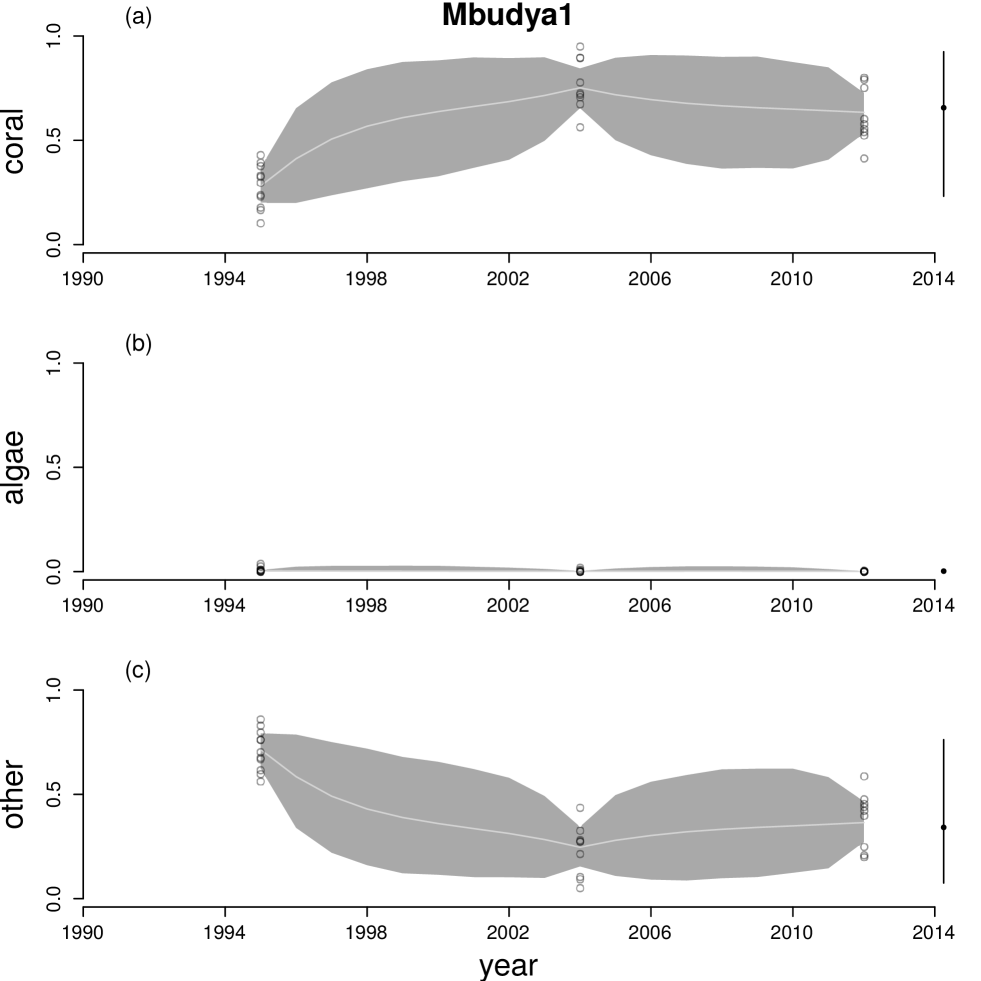
Figure A29: Time series for cover of hard corals (a), macroalgae (b) and other (c) at Mbudya1. See Figure A12 legend for explanation.

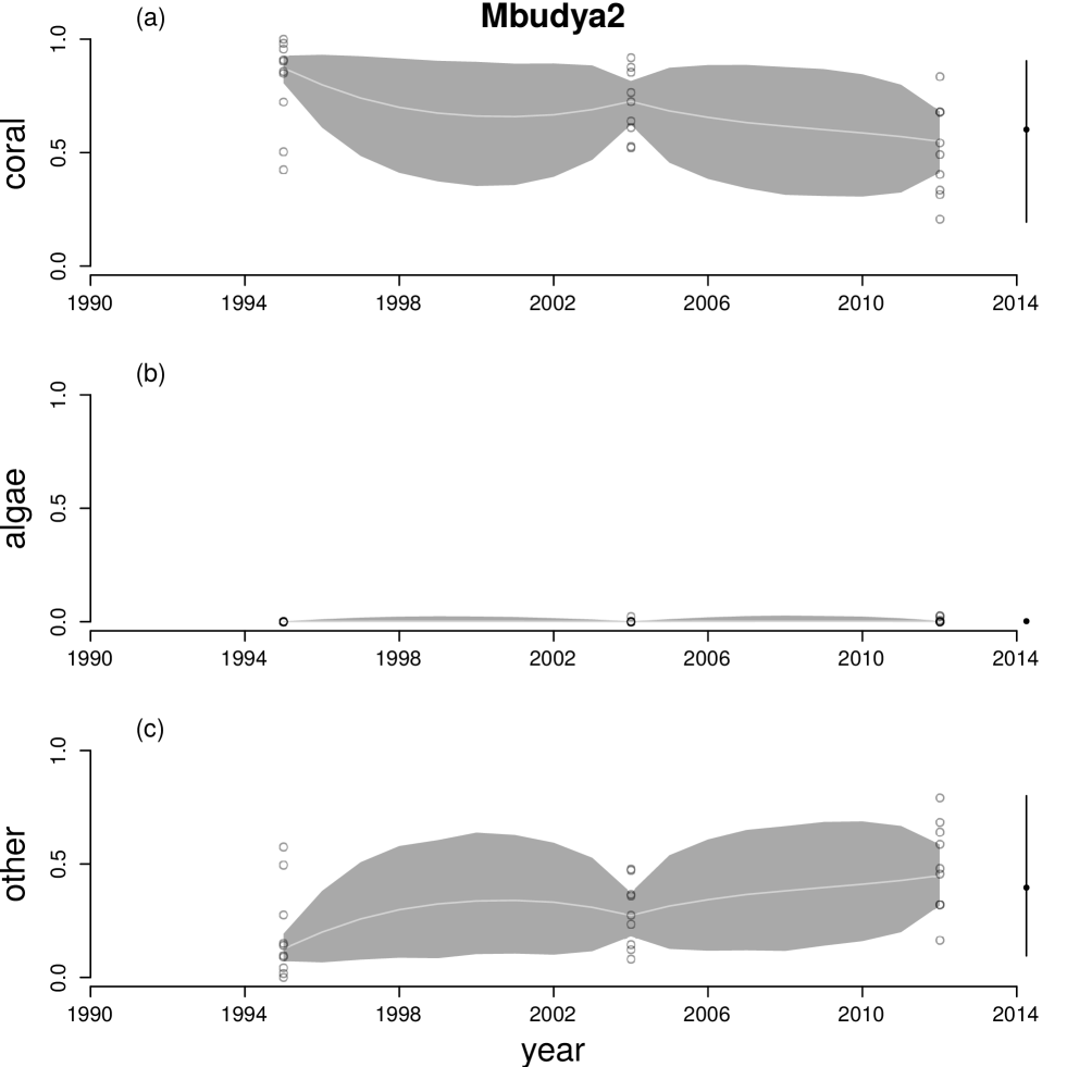
Figure A30: Time series for cover of hard corals (a), macroalgae (b) and other (c) at Mbudya2. See Figure A12 legend for explanation.

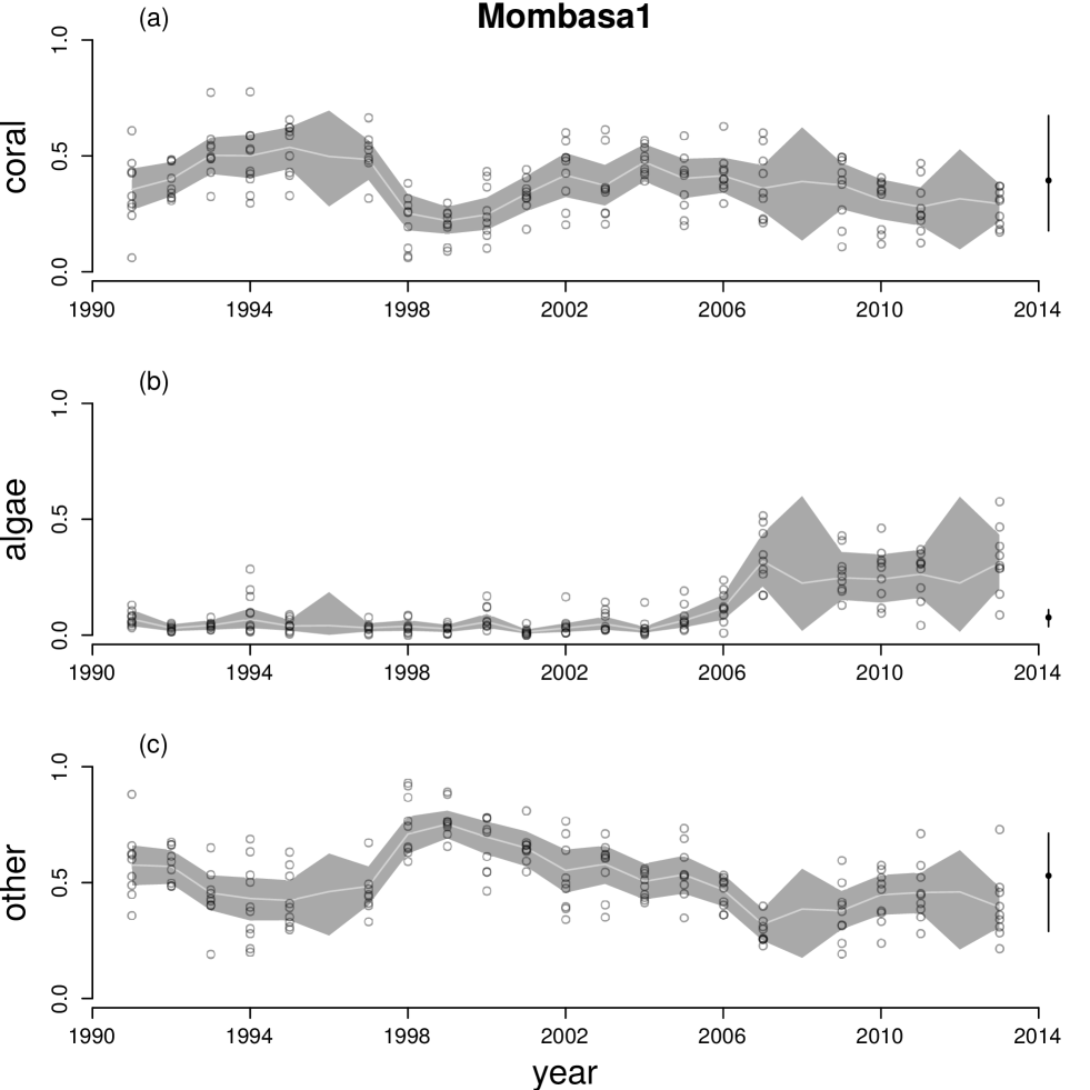
Figure A31: Time series for cover of hard corals (a), macroalgae (b) and other (c) at Mombasa1. See Figure A12 legend for explanation.

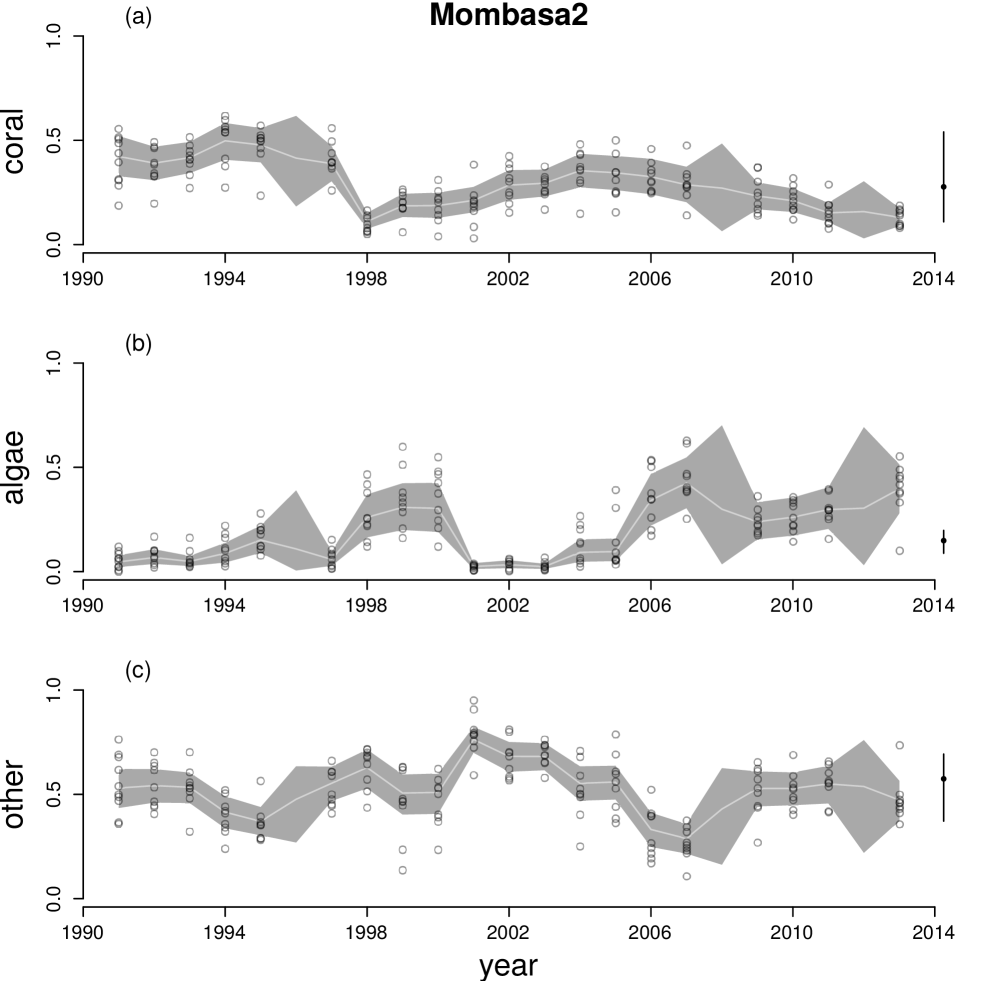
Figure A32: Time series for cover of hard corals (a), macroalgae (b) and other (c) at Mombasa2. See Figure A12 legend for explanation.

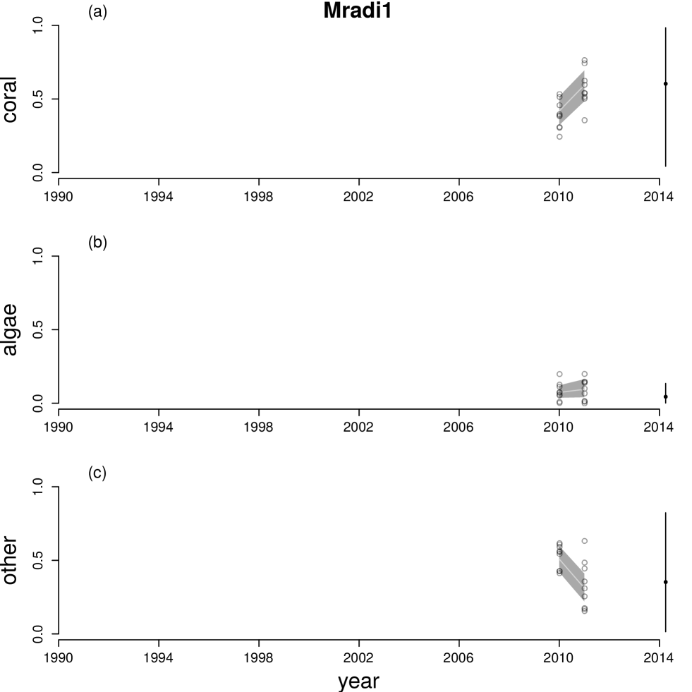
Figure A33: Time series for cover of hard corals (a), macroalgae (b) and other (c) at Mradi1. See Figure A12 legend for explanation.

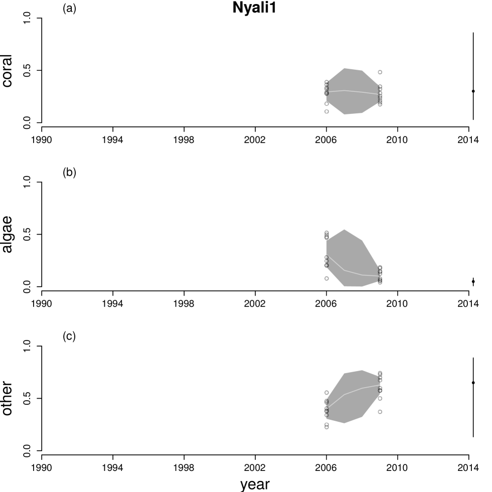
Figure A34: Time series for cover of hard corals (a), macroalgae (b) and other (c) at Nyali1. See Figure A12 legend for explanation.

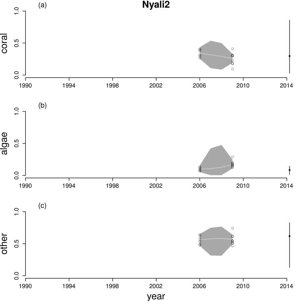
Figure A35: Time series for cover of hard corals (a), macroalgae (b) and other (c) at Nyali2. See Figure A12 legend for explanation.

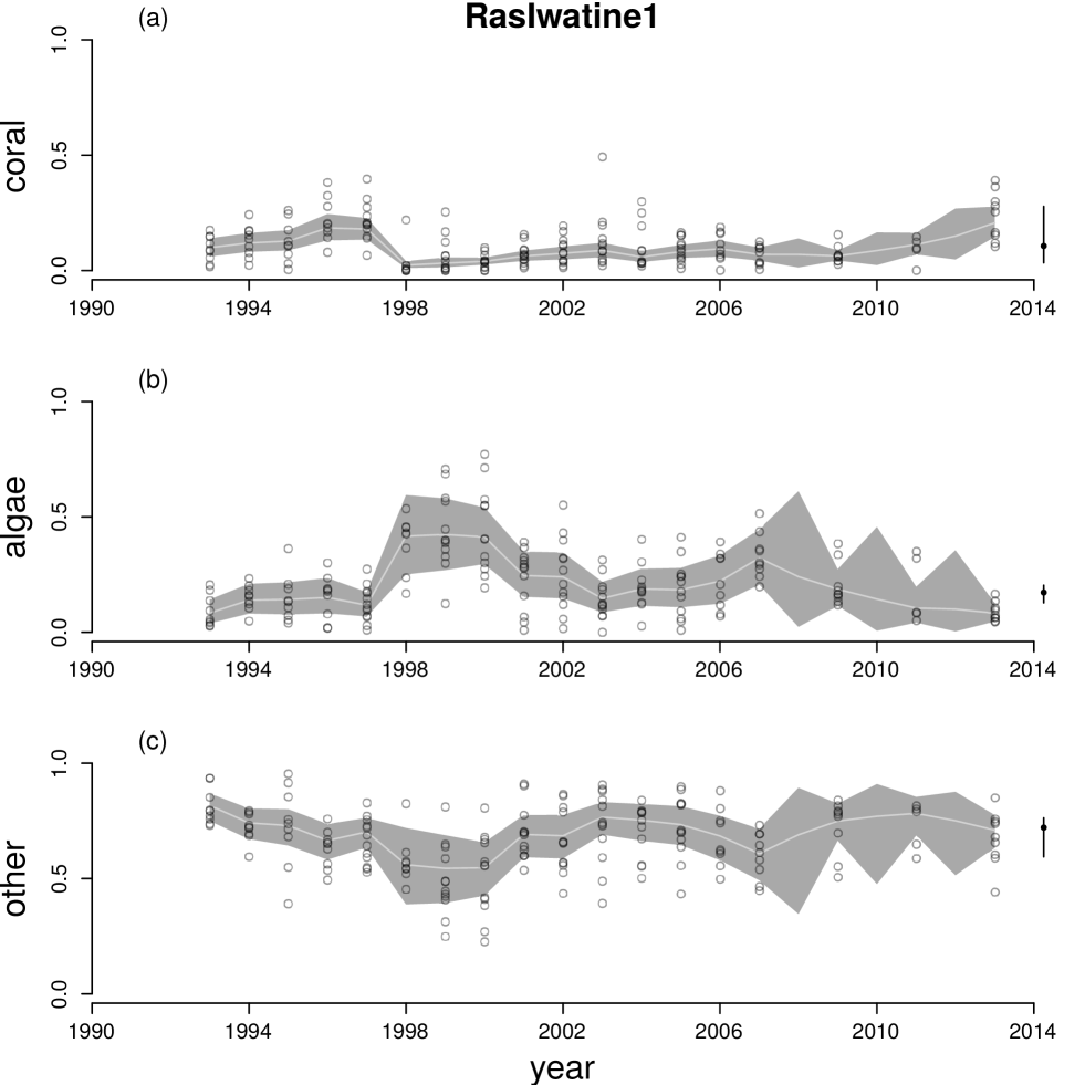
Figure A36: Time series for cover of hard corals (a), macroalgae (b) and other (c) at RasIwatine1. See Figure A12 legend for explanation.

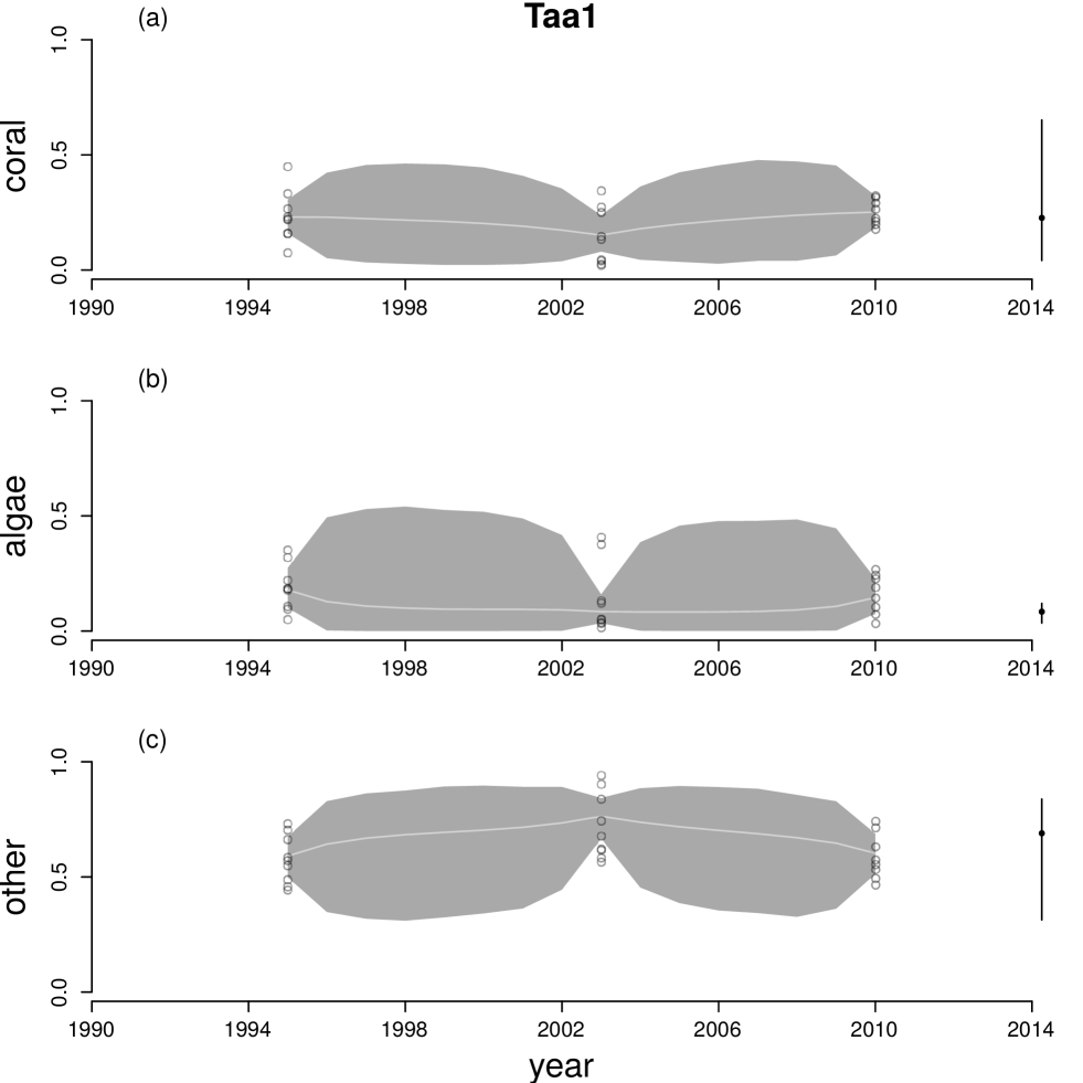
Figure A37: Time series for cover of hard corals (a), macroalgae (b) and other (c) at Taa1. See Figure A12 legend for explanation.

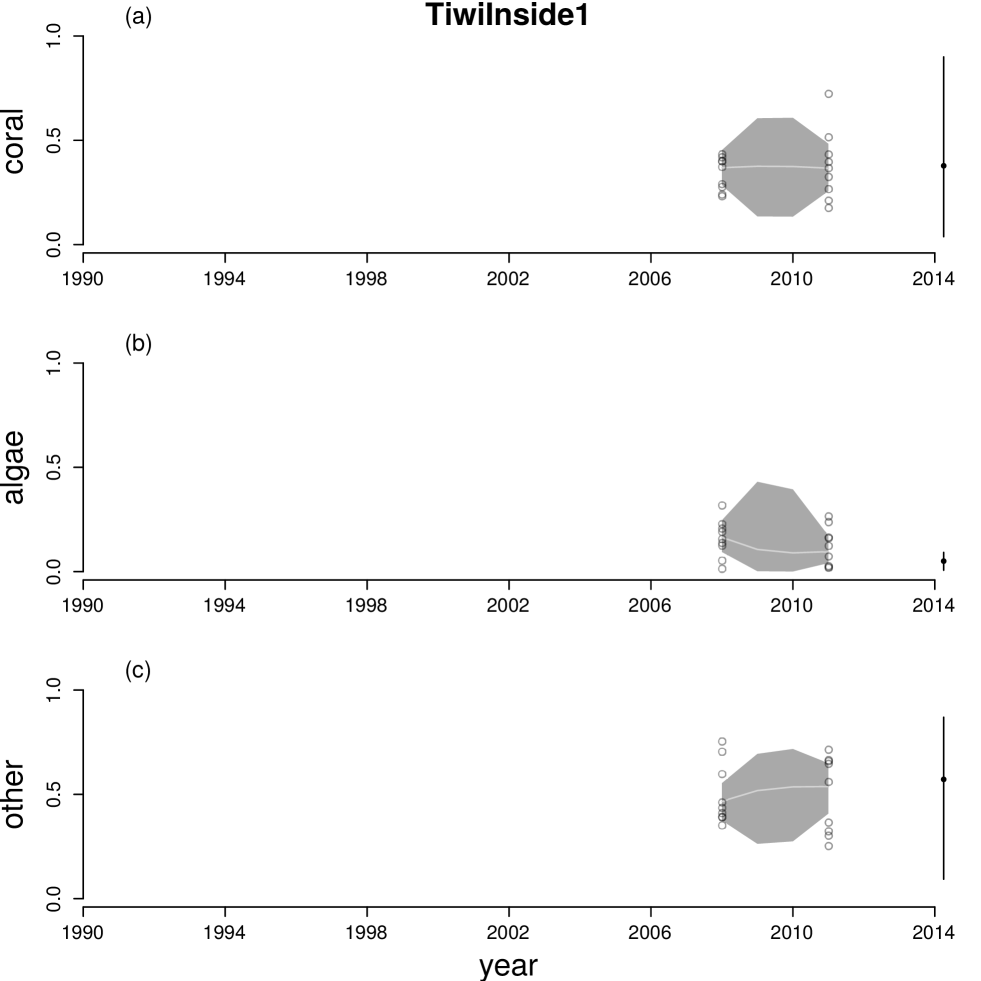
Figure A38: Time series for cover of hard corals (a), macroalgae (b) and other (c) at TiwiInside1. See Figure A12 legend for explanation.

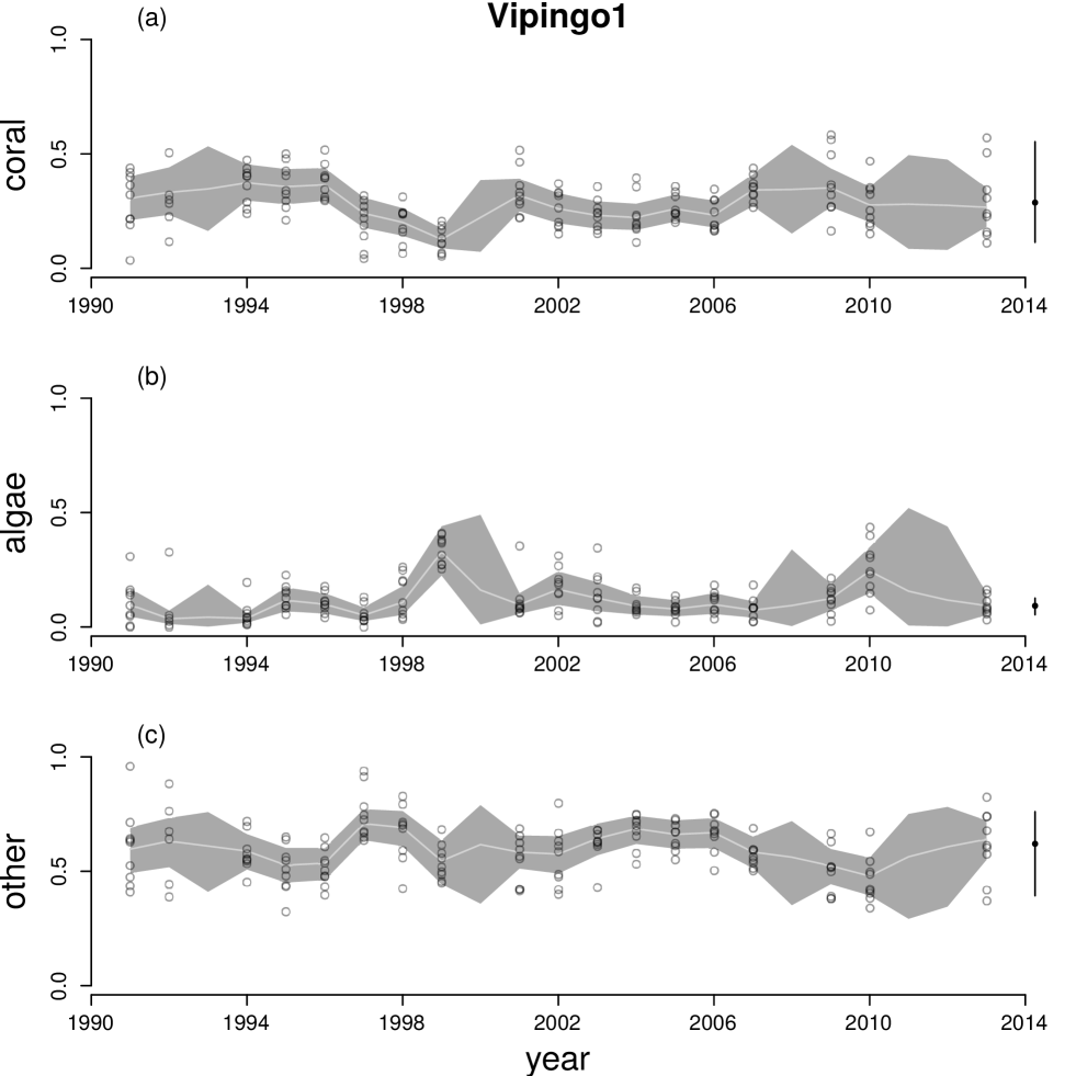
Figure A39: Time series for cover of hard corals (a), macroalgae (b) and other (c) at Vipingo1. See Figure A12 legend for explanation.

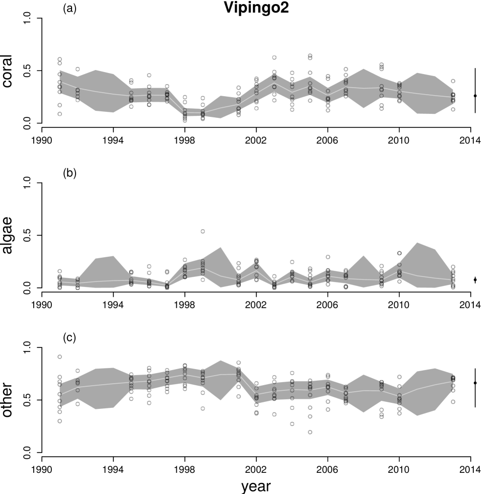
Figure A40: Time series for cover of hard corals (a), macroalgae (b) and other (c) at Vipingo2. See Figure A12 legend for explanation.

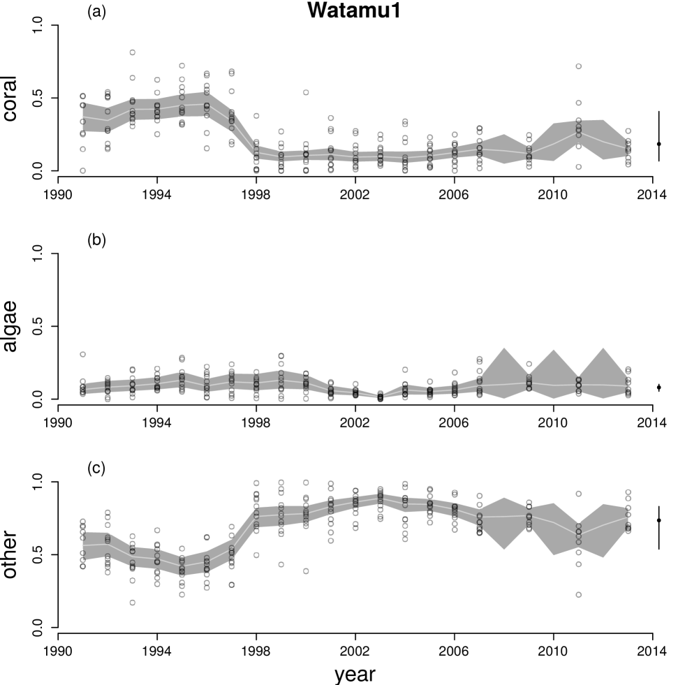
Figure A41: Time series for cover of hard corals (a), macroalgae (b) and other (c) at Watamu1. See Figure A12 legend for explanation.

Figure A48: Elements of the gradient vector of partial derivatives of the long-term probability of coral cover less than or equal to 0.2 with respect to elements of the $\mathbf{B}$ matrix, the $\mathbf{a}$ vector, the covariance matrix of random temporal variation $\bm{\Sigma}$, and the covariance matrix of among-site variability $\mathbf{Z}$. For each parameter, the dot is the posterior mean and the bar is a 95$\%$ HPD interval. For the covariance matrices, the elements $\sigma_{12}$ and $\zeta_{12}$ are not shown, because they are constrained to be equal to $\sigma_{21}$ and $\zeta_{21}$ respectively.

Figure A49: Ranks of partial derivatives of the long-term probability of coral cover less than or equal to 0.2 with respect to elements of the $\mathbf{B}$ matrix, the $\mathbf{a}$ vector, the covariance matrix of random temporal variation $\bm{\Sigma}$, and the covariance matrix of among-site variability $\mathbf{Z}$. Parameters are ranked in descending order of median rank (higher ranks indicate larger magnitudes of partial derivative). Outliers are indicated as jittered black dots. For the covariance matrices, the elements $\sigma_{12}$ and $\zeta_{12}$ are not shown, because they are constrained to be equal to $\sigma_{21}$ and $\zeta_{21}$ respectively.

Literature cited

- Aitchison, (1986) Aitchison, J. (1986). The statistical analysis of compositional data. Chapman and Hall, London.
- Aitchison, (1989) Aitchison, J. (1989). Measures of location for compositional data sets. Mathematical Geology, 21:787–790.
- Ateweberhan and McClanahan, (2016) Ateweberhan, M. and McClanahan, T. R. (2016). Partitioning scleractinian coral diversity across reef sites and regions in the Western Indian Ocean. Ecosphere, 7(5):01243.
- Auger-Méthé et al., (2015) Auger-Méthé, M., Field, C., Albertsen, C. M., Derocher, A. E., Lewis, M. A., Jonsen, I. D., and Mills Flemming, J. (2015). State-space models’ dirty little secrets: even simple linear Gaussian models can have estimation problems. unpublished, arXiv:1508.04325v1.
- Baker et al., (2008) Baker, A. C., Glynn, P. W., and Riegl, B. (2008). Climate change and coral reef bleaching: an ecological assessment of long-term impacts, recovery trends and future outlook. Estuarine, Coastal and Shelf Science, 80:435–471.
- Bjørnstad and Falck, (2001) Bjørnstad, O. N. and Falck, W. (2001). Nonparametric spatial covariance functions: Estimation and testing. Environmental and Ecological Statistics, 8:53–70.
- Brook et al., (2000) Brook, B. W., O’Grady, J. J., Chapman, A. P., Burgman, M. A., Akçakaya, H. R., and Frankham, R. (2000). Predictive accuracy of population viability analysis in conservation biology. Nature, 404:385–387.
- Bruno et al., (2009) Bruno, J. F., Sweatman, H., Precht, W. F., Selig, E. R., and Schutte, V. G. W. (2009). Assessing evidence of phase shifts from coral to macroalgal dominance on coral reefs. Ecology, 90(6):1478–1484.
- Carreiro-Silva and McClanahan, (2012) Carreiro-Silva, M. and McClanahan, T. R. (2012). Macrobioerosion of dead branching Porites, 4 and 6 years after coral mass mortality. Marine Ecology Progress Series, 458:103–122.
- Caswell, (2001) Caswell, H. (2001). Matrix population models: construction, analysis, and interpretation. Sinauer, Sunderland, MA, second edition.
- Cinner and McClanahan, (2015) Cinner, J. E. and McClanahan, T. R. (2015). A sea change on the African coast? Preliminary social and ecological outcomes of a governance transformation in Kenyan fisheries. Global Environmental Change, 30:133–139.
- Connell et al., (1997) Connell, J. H., Hughes, T. P., and Wallace, C. C. (1997). A 30-year study of coral abundance, recruitment, and disturbance at several scales in space and time. Ecological Monographs, 67(4):461–488.
- Cooper et al., (2015) Cooper, J. K., Spencer, M., and Bruno, J. F. (2015). Stochastic dynamics of a warmer Great Barrier Reef. Ecology, 96:1802–1811.
- Côté et al., (2005) Côté, I. M., Gill, J. A., Gardner, T. A., and Watkinson, A. R. (2005). Measuring coral reef decline through meta-analyses. Philosophical Transactions of the Royal Society Series B, 360:385–395.
- De’ath et al., (2012) De’ath, G., Fabricius, K. E., Sweatman, H., and Puotinen, M. (2012). The 27-year decline of coral cover on the Great Barrier Reef and its causes. Proceedings of the National Academy of Sciences of the USA, 109:17995–17999.
- Diamond, (1986) Diamond, J. (1986). Overview: laboratory experiments, field experiments, and natural experiments. In Diamond, J. and Case, T. J., editors, Community ecology, pages 3–22. Harper & Row, New York.
- Egozcue et al., (2003) Egozcue, J. J., Pawlowsky-Glahn, V., Mateu-Figueras, G., and Barceló-Vidal, C. (2003). Isometric logratio transformations for compositional data analysis. Mathematical Geology, 35(3):279–300.
- Gelman et al., (2003) Gelman, A., Carlin, J. B., Stern, H. S., and Rubin, D. B. (2003). Bayesian Data Analysis. Chapman and Hall/CRC, Boca Raton, second edition.
- Ginzburg et al., (1982) Ginzburg, L. R., Slobodkin, L. B., Johnson, K., and Bindman, A. G. (1982). Quasiextinction probabilities as a measure of impact on population growth. Risk Analysis, 21:171–181.
- Gross and Edmunds, (2015) Gross, K. and Edmunds, P. J. (2015). Stability of Caribbean coral communities quantified by long-term monitoring and autoregression models. Ecology, 96:1812–1822.
- Hampton et al., (2013) Hampton, S. E., Holmes, E. E., Scheef, L. P., Scheuerell, M. D., Katz, S. L., Pendleton, D. E., and Ward, E. J. (2013). Quantifying effects of abiotic and biotic drivers on community dynamics with multivariate autoregressive (MAR) models. Ecology, 94(12):2663–2669.
- Henze and Zirkler, (1990) Henze, N. and Zirkler, B. (1990). A class of invariant consistent tests for multivariate normality. Communications in Statistics - Theory and Methods, 19:3595–3617.
- Hoffman and Gelman, (2014) Hoffman, M. D. and Gelman, A. (2014). The No-U-Turn Sampler: Adaptively setting path lengths in Hamiltonian Monte Carlo. Journal of Machine Learning Research, 15:1351–1381.
- Hyndman, (1996) Hyndman, R. J. (1996). Computing and graphing highest density regions. The American Statistician, 50(2):120–126.
- Ives et al., (2003) Ives, A. R., Dennis, B., Cottingham, K. L., and Carpenter, S. R. (2003). Estimating community stability and ecological interactions from time-series data. Ecological Monographs, 73(2):301–330.
- Johnson and Wichern, (2007) Johnson, R. A. and Wichern, D. W. (2007). Applied multivariate statistical analysis. Pearson, 6th edition.
- Kaiser, (1983) Kaiser, L. (1983). Unbiased estimation in line-intercept sampling. Biometrics, 39(4):965–976.
- Kennedy et al., (2013) Kennedy, E. V., Perry, C. T., Halloran, P. R., Iglesias-Prieto, R., Schönberg, C. H. L., Wissah, M., Form, A. U., Carricart-Ganivet, J. P., Fine, M., Eakin, C. M., and Mumby, P. J. (2013). Avoiding coral reef functional collapse requires local and global action. Current Biology, 23:912–918.
- Kenward, (1979) Kenward, M. G. (1979). An intuitive approach to the MANOVA test criteria. Journal of the Royal Statistical Society Series D, 28(3):193–198.
- Korkmaz et al., (2014) Korkmaz, S., Goksuluk, D., and Zararsiz, G. (2014). MVN: An R package for assessing multivariate normality. The R Journal, 6:151–162.
- Lange et al., (1989) Lange, K. L., Little, R. J. A., and Taylor, J. M. G. (1989). Robust statistical modeling using the t distribution. Journal of the American Statistical Association, 84:881–896.
- Lindegren et al., (2009) Lindegren, M., Möllmann, C., Nielsen, A., and Stenseth, N. C. (2009). Preventing the collapse of the Baltic cod stock through an ecosystem-based management approach. Proceedings of the National Academy of Sciences of the USA, 106(34):14722–14727.
- Lütkepohl, (1993) Lütkepohl, H. (1993). Introduction to multiple time series analysis. Springer-Verlag, Berlin, 2nd edition.
- Magnus and Neudecker, (2007) Magnus, J. R. and Neudecker, H. (2007). Matrix differential calculus with applications in statistics and econometrics. John Wiley & Sons, Chichester, third edition.
- Mardia, (1970) Mardia, K. V. (1970). Measures of multivariate skewnees and kurtosis with applications. Biometrika, 57:519–530.
- Martín-Fernández et al., (2003) Martín-Fernández, J. A., Barceló-Vidal, C., and Pawlowsky-Glahn, V. (2003). Dealing with zeros and missing values in compositional data sets using nonparametric imputation. Mathematical Geology, 35(3):253–278.
- McClanahan and Arthur, (2001) McClanahan, T. R. and Arthur, R. (2001). The effect of marine reserves and habitat on populations of East African coral reef fishes. Ecological Applications, 11(2):559–569.
- McClanahan et al., (2007) McClanahan, T. R., Ateweberhan, M., Muhando, C. A., Maina, J., and Mohammed, M. S. (2007). Effects of climate and seawater temperature variation on coral bleaching and mortality. Ecological Monographs, 77(4):503–525.
- McClanahan et al., (2016) McClanahan, T. R., Muthiga, N. A., and Abunge, C. A. (2016). Establishment of community managed fisheries’ closures in Kenya: early evolution of the tengefu movement. Coastal Management, 44:1–20.
- McClanahan et al., (2001) McClanahan, T. R., Muthiga, N. A., and Mangi, S. (2001). Coral and algal changes after the 1998 coral bleaching: interaction with reef management and herbivores on Kenyan reefs. Coral Reefs, 19:380–391.
- Mellin et al., (2014) Mellin, C., Bradshaw, C. J. A., Fordham, D. A., and Caley, M. J. (2014). Strong but opposing -diversity-stability relationships in coral reef fish communities. Proceedings of the Royal Society of London Series B, 281:20131993.
- Mirsky, (1955) Mirsky, L. (1955). An introduction to linear algebra. Oxford University Press, Oxford.
- Mumby et al., (2007) Mumby, P. J., Hastings, A., and Edwards, H. J. (2007). Thresholds and the resilience of Caribbean coral reefs. Nature, 450:98–101.
- Mutshinda et al., (2009) Mutshinda, C. M., O’Hara, R. B., and Woiwod, I. P. (2009). What drives community dynamics? Proceedings of the Royal Society of London Series B, 276:2923–2929.
- Otto and Day, (2007) Otto, S. P. and Day, T. (2007). A biologist’s guide to mathematical modeling in ecology and evolution. Princeton University Press, Princeton, New Jersey.
- Perry et al., (2013) Perry, C. T., Murphy, G. N., Kench, P. S., Smithers, S. G., Edinger, E. N., Steneck, R. S., and Mumby, P. J. (2013). Caribbean-wide decline in carbonate production threatens coral reef growth. Nature Communications, 4:1402.
- Piessens et al., (1983) Piessens, R., de Doncker-Kapenga, E., Überhuber, C. W., and Kahaner, D. (1983). QUADPACK: a subroutine package for automatic integration. Springer-Verlag, Berlin.
- R Core Team, (2015) R Core Team (2015). R: A Language and Environment for Statistical Computing. R Foundation for Statistical Computing, Vienna, Austria.
- Riley et al., (2002) Riley, K. F., Hobson, M. P., and Bence, S. J. (2002). Mathematical methods for physics and engineering. Cambridge University Press, Cambridge, second edition.
- Roff et al., (2015) Roff, G., Zhao, J.-X., and Mumby, P. J. (2015). Decadal-scale rates of reef erosion following El Niño-related mass coral mortality. Global Change Biology, 21:4415–4424.
- Royston, (1982) Royston, J. (1982). An extension of Shapiro and Wilk’s test for normality to large samples. Applied Statistics, 31:115–124.
- Sandin et al., (2008) Sandin, S. A., Smith, J. E., DeMartini, E. E., Dinsdale, E. A., Donner, S. D., Friedlander, A. M., Konotchick, T., Malay, M., Maragos, J. E., Obura, D., Pantos, O., Paulay, G., Richie, M., Rohwer, F., Schroeder, R. E., Walsh, S., Jackson, J. B. C., Knowlton, N., and Sala, E. (2008). Baselines and degradation of coral reefs in the Northern Line Islands. PLoS ONE, 3(2):e1548.
- (53) Stan Development Team (2015a). Stan: A C++ library for probability and sampling, version 2.7.0.
- (54) Stan Development Team (2015b). Stan Modeling Language Users Guide and Reference Manual, Version 2.7.0.
- Vehtari et al., (2015) Vehtari, A., Gelman, A., and Gabry, J. (2015). Efficient implementation of leave-one-out cross-validation and WAIC for evaluating fitted Bayesian models. unpublished, arXiv:1507.04544v1.
- Vercelloni et al., (2014) Vercelloni, J., Caley, M. J., Kayal, M., Low-Choy, S., and Mengersen, K. (2014). Understanding uncertainties in non-linear population trajectories: a Bayesian semi-parametric hierarchical approach to large-scale surveys of coral cover. PLoS ONE, 9(11):e110968.
- Wilks, (1932) Wilks, S. S. (1932). Certain generalizations in the analysis of variance. Biometrika, 24:471–494.
- Żychaluk et al., (2012) Żychaluk, K., Bruno, J. F., Clancy, D., McClanahan, T. R., and Spencer, M. (2012). Data-driven models for regional coral-reef dynamics. Ecology Letters, 15:151–158.