DESY 16-114

A new view on vacuum stability in the MSSM

Wolfgang Gregor Hollik

Deutsches Elektronen-Synchrotron (DESY)

Notkestraße 85, D-22607 Hamburg, Germany

A consistent theoretical description of physics at high energies requires an assessment of vacuum stability in either the Standard Model or any extension of it. Especially supersymmetric extensions allow for several vacua and the choice of the desired electroweak one gives strong constraints on the parameter space. As the general parameter space in the Minimal Supersymmetric Standard Model is huge, any severe constraint on it unrelated to direct phenomenological observations enhances the predictability of the model. We perform an updated analysis of possible charge and color breaking minima without relying on fixed directions in field space that minimize certain terms in the potential (known as “$D$-flat” directions). Concerning the cosmological stability of false vacua, we argue that there are always directions in configuration space which lead to very short-lived vacua and therefore such exclusions are strict. In addition to existing strong constraints on the parameter space, we find even stronger constraints extending the field space compared to previous analyses and combine those constraints with predictions for the light CP-even Higgs mass in the Minimal Supersymmetric Standard Model. Low masses for supersymmetric partners are excluded from vacuum stability in combination with the $125\,\mathrm{GeV}$ Higgs and the allowed parameter space opens at a few $\mathrm{TeV}$.

Keywords: Mostly Weak Interactions: Beyond Standard Model, Supersymmetric Standard Model
PACS: 11.15.Ex, 11.30.Pb, 12.60.Jv

1 Introduction

The Standard Model (SM) of particle physics is completed with the final discovery of the Higgs boson (the SM scalar) [1, 2] which shows the expected properties in the experiment [3] and only leaves small room for deviations from the SM predictions. However, this discovery finalized a set of problems within the SM from which one is the hierarchy problem of the Higgs mass [4, 5, 6, 7] another one the discussion about the cosmological stability of the electroweak ground state [8, 9, 10, 11, 12, 13, 14, 15, 16]. Surprisingly, the most popular extension of the SM to solve the hierarchy problem simultaneously cures the stability problem, which is the Minimal Supersymmetric Standard Model (MSSM). Besides the well-known solution of the hierarchy problem by the existence of bosonic degrees of freedom that cancel loop contributions, similar contributions render the effective potential stable—besides the property of the MSSM having an intrinsically stable Higgs potential at the tree-level. This solution to all problems, however, comes along with a bunch of new problems from which a prominent one in connection to the stability of the vacuum state is the possible destabilization of the Higgs potential by additional scalar degrees of freedom. Finally, the true vacuum of the theory is related to the absolute ground state of the scalar potential which is not exclusively dedicated to vacuum expectation values (vevs) of Higgs scalars anymore but can be due to vevs of the additional scalars that break electric and/or color charge and/or additionally baryon and lepton number. While spontaneous breaking of lepton number may be a desired solution to the origin of neutrino masses [17, 18, 19, 20], the spontaneous breakdown of good gauge symmetries in the SM should be avoided in a way that $\mathrm{SU}(3)_{c}\times\mathrm{U}(1)_{\text{em}}$ stays intact.

It was already noticed in the early 1980s [21] that supersymmetric models tend to have charge breaking minima and in the following rather strong constraints on the soft breaking terms have been derived [22, 23, 24, 25, 26, 27]. Subsequently, many attempts have been performed to improve such kind of bounds using several optimization criteria [28], higher loop effects [29, 30, 31, 32], relaxing constraints allowing for metastable states [33, 34], constraining flavor violation [35] and applying metastability constraints on the flavor violating bounds [36]. A sophisticated collection of codes checking for non-standard tree-level minima, improving with the one-loop effective potential and calculating tunneling rates in presence of finite temperatures by the help of CosmoTransitions [37] is given by the Vevacious collaboration [38]. Recently, the old charge and color breaking (CCB) constraints have been analyzed and tested in the light of the Higgs discovery at the LHC [39, 40] with an updated tunneling analysis [41]. An investigation of the one-loop Higgs potential in the MSSM [42] reveals an interrelation of one-loop stability constraints from the Higgs sector only and tree-level CCB constraints including colored directions [43]. Considerations of vacuum stability are a widely used ingredient in studies of MSSM-like scenarios [44, 45, 46, 47, 48].

A general paradigm is that charge and color breaking minima in the MSSM most probably appear in such directions in field space where the $D$-terms vanish. $D$-terms are the quadrilinear contributions to the full scalar potential proportional to squared gauge couplings and therefore always positive and always seen as to win over any negative contribution. A first more complete and rather exhaustive analysis taking basically all directions in field space into account was given about twenty years ago by [27], where a full list of many special cases had been discussed.

Still, a complete analysis of the problem that somehow resides in a satisfactory solution is not possible. We provide a possible way to handle the existence of non-standard vacua in the MSSM scalar potential that follows the spirit of [27] and goes beyond. The minimization procedure reduces then effectively to the optimization of the necessary condition for the existence on non-standard vacua. This optimization, however, is neither unique nor unambiguously to be determined. Moreover, once the vacuum tunneling probability is addressed, a new concern for the “optimized” field direction may arise: to give the strongest bound from the vacuum metastability, configurations are rather preferred that lead to the minimal tunneling time. Whether or not this requirement can be exploited in automated computer tools may be left to the programming skills of the developers. For the pedestrian, it appears sufficient to have a clear analytical cut although those rules are indeed not sufficient but necessary. This analytical cut, however, should only distinguish between a global CCB minimum and a strictly stable “desired” electroweak vacuum.

Why is a reassessment of this problem needed? Besides the complete analysis of [27] not so much has been done on the analytical level as it is quite hard and any access lacks generality. Since this great catalog of dangerous directions and associated bounds on the parameters has been worked out, the greatest further achievement is the discovery of the Higgs boson [2, 1] that appears to be very SM-like and has (for MSSM purposes) a rather high mass of $m_{h^{0}}=125\,\mathrm{GeV}$ as follows from the combination of ATLAS and CMS data at $7$ and $8\,\mathrm{TeV}$ [49]. This value requires sizeable radiative corrections, that are known to be large in the MSSM [50, 51]. However, the available parameter space gets very much constraint imposing the correct Higgs mass, even if one allows for a generous theoretical error of about $3\,\mathrm{GeV}$ in the determination of this mass [52]. Especially, to achieve this shift a large stop mixing is needed which conversely requires large trilinear soft SUSY breaking couplings [53, 54], assisted maybe by a large Higgsino mass parameter. These large trilinear scalar terms, however, unambiguously lead to CCB minima and render the desired vacuum unstable. It is therefore necessary and important to put severe constraints on those terms in order to assure theoretical consistency. As long as there persists to be no discovery of any sparticles at the LHC, inferring larger lower bounds on the sparticle masses will also lead to possibly more stable configurations as larger SUSY masses themselves lead to larger shifts in the Higgs mass [52] without the need for large left-right squark mixing. Anyhow, compressed scenarios that might be hidden in the collider searches are likely to be in trouble with the stability bounds; especially if they tuned [55] in such a way to reproduce weird signatures [56, 57].

We proceed in this paper as follows: after introducing the four-field scalar potential, which is basically the necessary object to deal with in connection to the influence on the Higgs mass, we derive a generic exclusion bound in Section 2. The anatomy of the CCB states described by this bound is discussed in Section 3. Finally, we conclude.

2 The four-field scalar potential

The MSSM in fact is a multi-scalar theory and its scalar potential is a complicated object potentially leading to undesired configurations. The configuration space depends on the vacuum expectation values of each field that are the field values at the minima of the potential. The potential in general has multiple minima where only the global one is considered to be the true ground state of the theory. If in any case the current electroweak vacuum we are believing to be sitting in is not the true one, this configuration will only be stable for a certain amount of time and due to quantum tunneling the global minimum will be reached. Moreover, we have to take care that the potential is not unbounded from below (constraints known as UFB, i. e. unbounded from below bounds in the literature). Taking quantum corrections (and at least the one-loop effective potential) into account, those will always be rescued and the quantum potential will be bounded from below [27, 42, 58], whereas a new deep minimum will appear at very large field values. Contrary to large field-valued minima that usually come along with low tunneling rates into the true ground state, the minima discussed in this paper are close-by roughly with vevs around the SUSY scale (few $\mathrm{TeV}$).

We are especially interested in the cross-relations of current analyses in the MSSM Higgs sector with the formation of non-standard vacua. The missing observational evidence for SUSY partners at all paired with a relatively heavy SM-like Higgs requests extreme parameter configurations. Existing analytical and semi-analytical bounds on the parameter space from the stability of the standard electroweak vacuum still are in agreement with what is needed to cope with the current situation. However, as we will see, most scenarios in the phenomenological MSSM (pMSSM) where all parameters are defined as input values at the SUSY scale suffer from charge and color breaking minima already at the SUSY scale (or slightly above). Moreover, the usual argument that tunneling rates to the deeper minimum are sufficiently small does not hold as there can be always a path in field space found where a closer vacuum shows up and fast tunneling proceeds to rolling down towards the final true vacuum. We shall explain this further.

Knowing the ground state of the theory means knowing the origin of spontaneous symmetry breaking means knowing the structure of the scalar potential. Each non-vanishing vev of fermionic or vector component fields would in addition break Lorentz symmetry and destroy the structure of space-time. Only the scalar part can break inner symmetries spontaneously and in a way which keeps external symmetries intact (not to speak about supersymmetry, but to break it we rely on soft breaking and stay ignorant about its deeper origin). The ground state of the theory is given by the state which minimizes the potential energy density; therefore the relevant object is actually the effective potential, which at tree-level is equivalent to the classical scalar potential. In principle, quantum (one and higher loop) effects are calculable [59, 60] and allow for spontaneous breaking radiatively. While the SM effective potential can be trivially made stable at the tree-level by choosing the Higgs self-coupling positive, the same coupling runs negative at higher energies and renders the electroweak vacuum metastable on cosmological scales [9, 61]. In multi-scalar theories as in the MSSM, the situation is more involved already at the tree-level; a tree-level analysis of the scalar potential will result in regions of allowed parameters. Loop corrections are not expected to make unstable regions more stable around the scale of the relevant vev, although purely loop-induced minima may be missed.

The MSSM scalar potential is calculated according to some simple rules and consists of three basic contributions to which we will refer as the soft breaking, the $F$-term and the $D$-term contribution:

$$V=V_{\text{soft}}+V_{F}+V_{D}.$$ (1)

The soft breaking part breaks supersymmetry softly and mimics the couplings of the superpotential plus additional scalar mass terms, where the $F$-terms basically follow from the superpotential as derivatives with respect to the scalar components

$$V_{F}=\left|\frac{\partial\mathcal{W}}{\partial\phi}\right|^{2},$$ (2)

where the sum over all scalar degrees of freedom is implicitly assumed to keep a plain notation. In our discussion and analysis, we consider only the chiral supermultiplets of third generation quarks as they couple with comparably large Yukawa couplings (as superpotential parameters) to the Higgs sector and also their corresponding trilinear soft SUSY breaking couplings are assumed to be large. For cleanliness and a first understanding of the “new” phenomena hidden in an old setup, we leave leptons and their superpartners out of the game as we are primarily interested in the appearance of color breaking minima. The inclusion of third generation (s)leptons is, however, trivial and follows the same procedure. We then define the (reduced) superpotential of “our” version of the MSSM by

$$\mathcal{W}=\mu\;H_{\mathrm{d}}\cdot H_{\mathrm{u}}+y_{\mathrm{t}}\;H_{\mathrm{u}}\cdot Q_{\mathrm{L}}\bar{T}_{\mathrm{R}}-y_{\mathrm{b}}\;H_{\mathrm{d}}\cdot Q_{\mathrm{L}}\bar{B}_{\mathrm{R}},$$ (3)

where we denote the left-handed quark doublet as $Q_{\mathrm{L}}=(T_{\mathrm{L}},B_{\mathrm{L}})$ and the two Higgs doublets as $H_{\mathrm{d}}=(h_{\mathrm{d}}^{0},-h_{\mathrm{d}}^{-})$ and $H_{\mathrm{u}}=(h_{\mathrm{u}}^{+},h_{\mathrm{u}}^{0})$, respectively, and the $\mathrm{SU}(2)_{\mathrm{L}}$-invariant multiplication by the dot product. The $\mathrm{SU}(2)_{\mathrm{L}}$ singlets are put into the left-chiral supermultiplets $\bar{T}_{\mathrm{R}}=\{\tilde{t}_{\mathrm{R}}^{*},t_{\mathrm{R}}^{c}\}$ and $\bar{B}_{\mathrm{R}}=\{\tilde{b}_{\mathrm{R}}^{*},b_{\mathrm{R}}^{c}\}$, respectively.

Additionally, we have to break SUSY softly which is done in the usual way with scalar mass terms and trilinear couplings:

$$V_{\text{soft}}= \;m_{H_{\mathrm{d}}}^{2}|h_{\mathrm{d}}|^{2}+m_{H_{\mathrm{u}}}^{2}|h_{\mathrm{u}}|^{2}-\left(B_{\mu}h_{\mathrm{d}}\cdot h_{\mathrm{u}}+\text{h.\,c.\ }\right)$$ (4)

$$+{\tilde{Q}}_{\mathrm{L}}^{*}\tilde{m}_{Q}^{2}\tilde{Q}_{\mathrm{L}}+{\tilde{t}}_{\mathrm{R}}^{*}\tilde{m}_{t}^{2}\tilde{t}_{\mathrm{R}}+{\tilde{b}}_{\mathrm{R}}^{*}\tilde{m}_{b}\tilde{b}_{\mathrm{R}}+\left(A_{\mathrm{t}}h_{\mathrm{u}}{\tilde{t}}_{\mathrm{L}}^{*}\tilde{t}_{\mathrm{R}}+A_{\mathrm{b}}h_{\mathrm{d}}{\tilde{b}}_{\mathrm{L}}^{*}\tilde{b}_{\mathrm{R}}+\text{h.\,c.\ }\right).$$

The $D$-term part, finally, gives additional quadrilinear terms for the scalar potential associated with gauge couplings,

$$V_{D}=\frac{g_{1}^{2}}{2}\left(\phi^{\dagger}\frac{\Upsilon_{\phi}}{2}\phi\right)^{2}+\frac{g_{2}^{2}}{2}\left(\phi^{\dagger}\frac{\sigma}{2}\phi\right)^{2}+\frac{g_{3}^{2}}{2}\left(\phi^{\dagger}\frac{T}{2}\phi\right)^{2},$$ (5)

with the corresponding hypercharges $\Upsilon_{\phi}$, weak charges $\sigma$ (Pauli matrices for $\mathrm{SU}(2)_{\mathrm{L}}$-doublets $\phi$) and color charge matrices $T$. Again, summation over all gauge multiplets $\phi$ is implicitly understood.

The charged Higgs directions play no role in the forthcoming discussion since on one hand the potential is $\mathrm{SU}(2)$-invariant and may be always rotated into the desired shape—on the other hand, the soft SUSY breaking terms also break $\mathrm{SU}(2)$ in the squark sector (as top and bottom squarks are treated differently and additional left-right mixing is introduced by the $A$-terms). Any charge breaking Higgs vev will then be related to a color breaking squark vev anyway and we shall be able to express everything in neutral Higgs vevs, $h_{\mathrm{d}}^{0}$ and $h_{\mathrm{u}}^{0}$ (for simplicity, we drop the superscript “⁰” in the following), as well as stop and sbottom vevs $\tilde{t}$ and $\tilde{b}$. Finally, we have the combined top/bottom-squark–Higgs scalar potential

$$V_{\tilde{q},h}= {\tilde{t}}_{\mathrm{L}}^{*}\left(\tilde{m}_{Q}^{2}+|y_{\mathrm{t}}h_{\mathrm{u}}|^{2}\right)\tilde{t}_{\mathrm{L}}+{\tilde{t}}_{\mathrm{R}}^{*}\left(\tilde{m}_{t}^{2}+|y_{\mathrm{t}}h_{\mathrm{u}}|^{2}\right)\tilde{t}_{\mathrm{R}}$$ (6)

$$+{\tilde{b}}_{\mathrm{L}}^{*}\left(\tilde{m}_{Q}^{2}+|y_{\mathrm{b}}h_{\mathrm{d}}|^{2}\right)\tilde{b}_{\mathrm{L}}+{\tilde{b}}_{\mathrm{R}}^{*}\left(\tilde{m}_{b}^{2}+|y_{\mathrm{b}}h_{\mathrm{d}}|^{2}\right)\tilde{b}_{\mathrm{R}}$$

$$-\left[{\tilde{t}_{\mathrm{L}}}^{*}\left(\mu^{*}y_{\mathrm{t}}\;h^{*}_{\mathrm{d}}-A_{\mathrm{t}}h_{\mathrm{u}}\right)\tilde{t}_{\mathrm{R}}+\text{h.\,c.\ }\right]-\left[{\tilde{b}_{\mathrm{L}}}^{*}\left(\mu^{*}y_{\mathrm{b}}\;h^{*}_{\mathrm{u}}-A_{\mathrm{b}}h_{\mathrm{d}}\right)\tilde{b}_{\mathrm{R}}+\text{h.\,c.\ }\right]$$

$$+|y_{\mathrm{t}}|^{2}|\tilde{t}_{\mathrm{L}}|^{2}|\tilde{t}_{\mathrm{R}}|^{2}+|y_{\mathrm{b}}|^{2}|\tilde{b}_{\mathrm{L}}|^{2}|\tilde{b}_{\mathrm{R}}|^{2}$$

$$+\frac{g_{1}^{2}}{8}\left(|h_{\mathrm{u}}|^{2}-|h_{\mathrm{d}}|^{2}+\frac{1}{3}|\tilde{b}_{\mathrm{L}}|^{2}+\frac{2}{3}|\tilde{b}_{\mathrm{R}}|^{2}+\frac{1}{3}|\tilde{t}_{\mathrm{L}}|^{2}-\frac{4}{3}|\tilde{t}_{\mathrm{R}}|^{2}\right)^{2}$$

$$+\frac{g_{2}^{2}}{8}\left(|h_{\mathrm{u}}|^{2}-|h_{\mathrm{d}}|^{2}+|\tilde{b}_{\mathrm{L}}|^{2}-|\tilde{t}_{\mathrm{L}}|^{2}\right)^{2}$$

$$+\frac{g_{3}^{2}}{8}\left(|\tilde{t}_{\mathrm{L}}|^{2}-|\tilde{t}_{\mathrm{R}}|^{2}+|\tilde{b}_{\mathrm{L}}|^{2}-|\tilde{b}_{\mathrm{R}}|^{2}\right)^{2}$$

$$+(m_{H_{\mathrm{u}}}^{2}+|\mu|^{2})|h_{\mathrm{u}}|^{2}+(m_{H_{\mathrm{d}}}^{2}+|\mu|^{2})|h_{\mathrm{d}}|^{2}-2\operatorname{Re}(B_{\mu}\;h_{\mathrm{d}}h_{\mathrm{u}}).$$

Some remarks are necessary on the structure of the scalar potential given above and how to treat the field values and their possible phases. In the previous honorable and groundbreaking works introducing charge and color breaking solutions for the first time [21, 22] it is correctly stated that for potentials considered in these cases, the trilinear couplings as well as the corresponding field vevs can always be chosen real and positive. This obvious observation, however, might be used to overconstrain the field space and therefore underconstrain the constraints on the involved parameters. Indeed, the potential of Eq. (6) has some freedom in the field redefinitions; especially, it is rephasing invariant apart from the trilinear terms and the Higgs bilinear $\sim B_{\mu}h_{\mathrm{d}}h_{\mathrm{u}}$. The last term is real by construction, all the others (besides the trilinears) are absolute squares of field values. Still, we do not have the freedom to rephase the fields in such a way, that the trilinear terms behave in a well defined way. In particular, the choice of all fields real and positive is not possible! We can, for sure, find a convention for the scalar quarks but not anymore for the Higgs fields. We therefore allow both $h_{\mathrm{u}}$ and $h_{\mathrm{d}}$ to vary in the positive and negative regime and only constrain $|\tilde{t}|=\alpha|\phi|$ as well as $|\tilde{b}|=\beta|\phi|$ with a certain scalar field value $\phi$ (where we choose $h_{\mathrm{u}}=\phi$). Moreover, we set $h_{\mathrm{d}}=\eta\phi$ with $\eta$ any real number and $\alpha$, $\beta$ real and positive. In case, we are considering real parameters only (not the complex MSSM), the potential is symmetric in $\mathrm{L}\leftrightarrow\mathrm{R}$ exchange of left- and right-handed field labels. Setting all squark fields $\tilde{q}_{\mathrm{L}}=\tilde{q}_{\mathrm{R}}$ (with $q=t,b$) simplifies also the $D$-terms in the sense, that the $g_{3}^{2}$ contribution vanishes and the $g_{2}^{2}$ and $g_{1}^{2}$ are the same in terms of the fields. The commitment to real parameters (and fields!) nevertheless is also a severe constraint, that may be, however, compassed by imposing global $\mathrm{CP}$-invariance of the theory (i. e.  $\mathrm{CP}$-invariance of SUSY breaking if one refers to the $A$-terms). It is therefore a good assumption to consider real fields only and just constrain the colored scalars to be positive (as the colored potential is invariant under $\tilde{q}\to-\tilde{q}$).

Applying the considerations from above, we now have

$$V_{\phi}= \alpha^{2}(\tilde{m}_{Q}^{2}+\tilde{m}_{t}^{2}+2y_{\mathrm{t}}^{2}\phi^{2})\phi^{2}+\beta^{2}(\tilde{m}_{Q}^{2}+\tilde{m}_{b}^{2}+2y_{\mathrm{b}}^{2}\eta^{2}\phi^{2})\phi^{2}$$ (7)

$$+\left(m_{H_{\mathrm{u}}}^{2}+\eta^{2}m_{H_{\mathrm{d}}}^{2}+(1+\eta^{2})|\mu|^{2}-2B_{\mu}\eta\right)\phi^{2}$$

$$-2\alpha^{2}(\mu y_{\mathrm{t}}\eta-A_{\mathrm{t}})\phi^{3}-2\beta^{2}(\mu y_{\mathrm{b}}-\eta A_{\mathrm{b}})\phi^{3}$$

$$(\alpha^{4}y_{\mathrm{t}}^{2}+\beta^{4}y_{\mathrm{b}}^{2})\phi^{4}+\frac{g_{1}^{2}+g_{2}^{2}}{8}\left(1-\eta^{2}+\beta^{2}-\alpha^{2}\right)^{2}\phi^{4},$$

where we applied in Eq. (6)

$$h_{\mathrm{u}}=\phi, |\tilde{t}_{\mathrm{L}}|=|\tilde{t}_{\mathrm{R}}|=|\tilde{t}|=\alpha|\phi|,$$ (8)

$$h_{\mathrm{d}}=\eta\phi, |\tilde{b}_{\mathrm{L}}|=|\tilde{b}_{\mathrm{R}}|=|\tilde{b}|=\beta|\phi|.$$

Rewriting finally the potential, we get

$$V_{\phi}= \left(m_{H_{\mathrm{u}}}^{2}+\eta^{2}m_{H_{\mathrm{d}}}^{2}+(1+\eta^{2})\mu^{2}-2B_{\mu}\eta+(\alpha^{2}+\beta^{2})\tilde{m}_{Q}^{2}+\alpha^{2}\tilde{m}_{t}^{2}+\beta^{2}\tilde{m}_{b}^{2}\right)\phi^{2}$$ (9)

$$-2\left(\alpha^{2}(\mu y_{\mathrm{t}}\eta-A_{\mathrm{t}})+\beta^{2}(\mu y_{\mathrm{b}}-\eta A_{\mathrm{b}})\right)\phi^{3}+(\alpha^{2}y_{\mathrm{t}}^{2}+\beta^{4}y_{\mathrm{b}}^{2})\phi^{4}$$

$$+\left(\frac{g_{1}^{2}+g_{2}^{2}}{8}(1-\eta^{2}+\beta^{2}-\alpha^{2})^{2}+2\alpha^{2}y_{\mathrm{t}}^{2}+2\beta^{2}y_{\mathrm{b}}^{2}\right)\phi^{4}$$

$$\equiv M^{2}\phi^{2}-\mathcal{A}\phi^{3}+\lambda\phi^{4},$$

with

$$M^{2} =\;m_{H_{\mathrm{u}}}^{2}+\eta^{2}m_{H_{\mathrm{d}}}^{2}-2B_{\mu}\eta+(1+\eta^{2})\mu^{2}+(\alpha^{2}+\beta^{2})\tilde{m}_{Q}^{2}+\alpha^{2}\tilde{m}_{t}^{2}+\beta^{2}\tilde{m}_{b}^{2}\,,$$ (10a)

$$\mathcal{A} =\;2\alpha^{2}\eta\mu y_{\mathrm{t}}-2\alpha^{2}A_{\mathrm{t}}+2\beta^{2}\mu y_{\mathrm{b}}-2\eta\beta^{2}A_{\mathrm{b}}\,,$$ (10b)

$$\lambda =\;\frac{g_{1}^{2}+g_{2}^{2}}{8}(1-\eta^{2}+\beta^{2}-\alpha^{2})^{2}+(2+\alpha^{2})\alpha^{2}y_{\mathrm{t}}^{2}+(2\eta^{2}+\beta^{2})\beta^{2}y_{\mathrm{b}}^{2}\,.$$ (10c)

Each of the effective parameters in the potential Eq. (9) depends implicitly on the scaling parameters, so $M^{2}=M^{2}(\eta,\alpha,\beta)$, $\mathcal{A}=\mathcal{A}(\eta,\alpha,\beta)$ and $\lambda=\lambda(\eta,\alpha,\beta)$. The minimization of the one field potential is done trivially and also the requirement for the global minimum at $\langle\phi\rangle=0$ is known to be

$$M^{2}>\frac{\mathcal{A}^{2}}{4\lambda}.$$

Knowing about the dependence on the actual field direction, this bound can be improved as

$$4\min_{\{\eta,\alpha,\beta\}}\lambda(\eta,\alpha,\beta)M^{2}(\eta,\alpha,\beta)>\max_{\{\eta,\alpha,\beta\}}\left(\mathcal{A}(\eta,\alpha,\beta)\right)^{2},$$ (11)

or rather

$$\min_{\{\eta,\alpha,\beta\}}\left[4\lambda(\eta,\alpha,\beta)M^{2}(\eta,\alpha,\beta)-\left(\mathcal{A}(\eta,\alpha,\beta)\right)^{2}\right]>0.$$

Note, that we easily recover the famous “traditional” CCB bound by Frère et al. [21] setting $\eta=\beta=0$ and $\alpha=1$ which corresponds to the ray $|\tilde{t}_{\mathrm{L}}|=|\tilde{t}_{\mathrm{R}}|=|h_{\mathrm{u}}|$ in field space: $M^{2}(0,1,0)=m_{H_{\mathrm{u}}}^{2}+\mu^{2}+{\tilde{m}}_{Q}^{2}+{\tilde{m}}_{t}^{2}$, $\mathcal{A}(0,1,0)=-2A_{\mathrm{t}}$ and $\lambda(0,1,0)=3y_{\mathrm{t}}^{2}$, such that

$$|A_{\mathrm{t}}|^{2}<3y_{\mathrm{t}}^{2}\left(m_{H_{\mathrm{u}}}^{2}+\mu^{2}+{\tilde{m}}_{L}^{2}+{\tilde{m}}_{t}^{2}\right).$$ (12)

Similar expressions can be easily achieved for different field directions. The specific choices have been made to make all gauge coupling contributions in Eq. (10c) vanish—though the quartics from the Yukawa couplings, which are numerically much larger, remain. There exists no real solution for $\eta$ with non-vanishing $\alpha$ and/or $\beta$ to have $\lambda=0$. So there will be (large) quartics anyway, which on the other hand means that we do not necessarily need to restrict to the $D$-flat condition which explicitly forces all $g_{i}^{2}$-terms in the scalar potential to be absent.

Similarly, by employing other alignments, we also recover the recently proposed [43] $\mu y_{\mathrm{b}}$ bound and the corresponding bound from the $h_{\mathrm{u}}$-$\tilde{b}$ $D$-flat direction with either $\eta=0$ and $\beta=1$,

$$\frac{\left(\mu y_{\mathrm{b}}\right)^{2}}{y_{\mathrm{b}}^{2}+(g_{1}^{2}+g_{2})^{2}/2}<m_{H_{\mathrm{u}}}^{2}+\mu^{2}+{\tilde{m}}_{Q}^{2}+{\tilde{m}}_{b}^{2},$$ (13)

or $h_{\mathrm{d}}=\pm\sqrt{1+\alpha^{2}}|h_{\mathrm{u}}|$, corresponding to $|h_{\mathrm{d}}|^{2}=|h_{\mathrm{u}}|^{2}+|\tilde{b}|^{2}$, and leading to

$$\frac{\alpha^{2}\mu^{2}}{2+3\alpha^{2}}<(1+\alpha^{2})m_{H_{\mathrm{d}}}^{2}+m_{H_{\mathrm{u}}}^{2}+(2+\alpha^{2})\mu^{2}\pm 2B_{\mu}^{2}\sqrt{1+\alpha^{2}}+\alpha^{2}\left({\tilde{m}}_{Q}^{2}+{\tilde{m}}_{b}^{2}\right),$$ (14)

with $\alpha>0$; a reasonable fit to the numerically derived exclusion limits can be found for $\alpha\approx 0.8$.

In the past, many attempts have been exercised to significantly improve the stability bound on the trilinear $A$-term according to Uneq. (12). Possible replacements range from

$$|A_{\mathrm{t}}|^{2}<3y_{\mathrm{t}}^{2}\left(m_{H_{\mathrm{u}}}^{2}+{\tilde{m}}_{Q}^{2}+{\tilde{m}_{t}}^{2}\right),$$ (15)

which was given (actually for $\mathrm{t}\leftrightarrow\mathrm{u}$ on the first generation $A$-term) by [27] and improved considering the cosmological stability of the potential through tunneling effects by [34] to

$$A_{\mathrm{t}}^{2}/y_{\mathrm{t}}^{2}+3\mu^{2}<7.5\left({\tilde{m}}_{Q}^{2}+{\tilde{m}_{t}}^{2}\right),$$ (16)

and recently updated by [41] in the light of the Higgs discovery as

$$A_{\mathrm{t}}^{2}/y_{\mathrm{t}}^{2}<3.4\left({\tilde{m}}_{Q}^{2}+{\tilde{m}}_{t}^{2}\right)+60\left(m_{h_{2}}^{2}+\mu^{2}\right),$$ (17)

which is more in agreement (numerically) with Uneq. (15) but shall only be applied to smaller values of $\mu$ and larger pseudoscalar masses $m_{A}$, whereas moderate $\tan\beta$. How exactly this “small”, “large” and “moderate” is defined may be left to the gusto of the user. All in all, the bounds (12)–(17) leave an undecided feeling behind and remain open the question for a robust, roughly unique and unambiguous constraint (which we also fail to provide).

We insist on the smaller sign ($<$) in Uneq. (12) and later on because the smaller or equal ($\leq$) includes a degenerate vacuum with $\langle\phi\rangle\neq 0$ which also leads to undesired phenomenology (where we do not want to speculate about multiple degenerate vacua as done for the SM Higgs case [62]). To be on the safe side, the $<$ is always preferred. The optimized class of conditions given in Uneq. (11) lead in general to a more involved interplay of different field directions that cannot be displayed in such a nice expression like Uneq. (12).

The meaning of such bounds stayed controversial in the literature and history. One significant improvement has been achieved by the discussion about the stability on cosmological grounds, the question whether or not the desired vacuum has had the possibility to decay to the true vacuum within the life-time of the universe. However, any (semi-)analytical constraint suffers from a distinct choice of the field configurations as any such choice influences the tunneling rate, as well.

The main task is now to find the “optimized” directions, meaning certain combinations of $\eta$, $\alpha$ and $\beta$ that give rise to the most severe bounds à la Uneq. (11) leading to the deepest CCB minimum (and therefore the true vacuum of the theory). Numerical minimization (and maximization) can be efficiently done with many available tools. However, as we will see, the optimized direction is not necessarily the most dangerous direction as the former one is in certain cases related to very large field vevs accompanied with a rather high barrier between the trivial (local) minimum at $\langle\phi\rangle=0$ and the true vacuum. Those configurations are related to very large tunneling times for the vacuum-to-vacuum transition and thus considered to be less dangerous. There are nevertheless slightly tilted or shifted directions in field space where the non-standard minimum lies closer and also the barrier is more complanate and therewith easier to be reached by quantum tunneling. Once the barrier is overcome, the true vacuum can be approached directly.

Before we continue with the actual analysis of the (reduced) MSSM incarnated in the full scalar potential of Eq. (6), we make a brief but necessary digression and discuss the issue of vacuum tunneling.

Instability vs. metastability

The process of finding the global minimum of a complicated potential is hazardous, even more the interpretation of the newly found configuration. Is the standard (local) vacuum stable against quantum tunneling towards this preferred true vacuum—or may there even be a path to gently roll down into the desired state? The estimate of the tunneling rate via the so-called bounce action itself is a tricky business, however, for a wide class of potentials a very pictorial approximation can be used where only the position (i.e. vev) of the deeper minimum and the maximum in between and the height of the wall is needed. For a thick wall separating the false from the true vacuum, a very convenient approximation formula was provided by [63] which is an exact solution for a triangular shape of the potential. The difficult part lies in the calculation of the bounce action $B$ [64], the decay rate per unit volume is then given by

$$\frac{\Gamma}{V}=Ae^{-B},$$

where $A$ is an undetermined amplitude factor, usually approximated by the false vev to the fourth power or the barrier height (as the uncertainty goes into the exponent, this does not really matter). The bounce itself depends in this approximation only on the true and the false vev, $\phi_{+}$ and $\phi_{-}$, respectively, the field value of the maximum in between $\phi_{M}$, and the values of the effective potential at the false vacuum $V_{+}=V(\phi_{+})$ as well as the peak of the wall $V_{M}=V(\phi_{M})$. The difference $\Delta V_{+}=V_{M}-V_{+}$ gives the height of the wall; furthermore, we define $\Delta\phi_{+}=\phi_{M}-\phi_{+}$ and $\Delta\phi_{-}=\phi_{-}-\phi_{M}$ and have the bounce action of [63]

$$B=\frac{2\pi^{2}}{3}\frac{\left[\left(\Delta\phi_{+}\right)^{2}-\left(\Delta\phi_{-}\right)^{2}\right]^{2}}{\Delta V_{+}}.$$ (18)

Eq. (18) is very convenient to check the stability of a given configuration in the reduced one-field potential without going into the details of the non-perturbative calculation. In comparison to the life-time of the universe, one finds metastable vacua for $B\gtrsim 400$, see [34].

Table 1: Input values and derived quantities for the two parameters points illustrated in Figs. 1 and 2.

	$M_{\text{SUSY}}$	$\tan\beta$	$\mu$	$A_{\mathrm{t}}=A_{\mathrm{b}}$	$m_{h^{0}}$	$B_{\text{global}}$
Fig. 1	$1\,\mathrm{TeV}$	$40$	$500\,\mathrm{GeV}$	$1500\,\mathrm{GeV}$	$126\,\mathrm{GeV}$	$354$
Fig. 2	$1\,\mathrm{TeV}$	$10$	$500\,\mathrm{GeV}$	$500\,\mathrm{GeV}$	$113\,\mathrm{GeV}$	$2568$

 

It is not necessarily the global minimum that determines the tunneling rate to a non-standard minimum. Numerical procedures may overlook the vacuum on one hand, but on the other hand the decay time to a local minimum may be much smaller and the transition to the deeper one does not play a role anymore. We want to illustrate at two sample points with different phenomenology that both show deeper charge and color breaking minima. The first point accounts for the proper Higgs mass with $m_{h^{0}}\approx 126\,\mathrm{GeV}$ where the other one would be discarded because it has $m_{h^{0}}\approx 113\,\mathrm{GeV}$. However, the nature of the global minimum is different for both points: while the first has a short-lived electroweak vacuum with $B\lesssim 400$, the other has an extremely long-lived false vacuum. All relevant parameters are given in Tab. 1. In all our analyses, we keep the pseudoscalar heavy to comply with the recent exclusions by collider searches for $A,H\to\tau\bar{\tau}$ [65, 66] and take $m_{A}=800\,\mathrm{GeV}$ (which is very borderline with the respect to the 2014 analyses up to $\tan\beta=40$ but unconstrained for smaller $\tan\beta=10$). The pseudoscalar mass has anyway only a mild impact on the charge and color breaking potential as it enters via the determination of the soft SUSY breaking Higgs masses $m_{H_{\mathrm{u}}}^{2}$, $m_{H_{\mathrm{d}}}^{2}$ and $B_{\mu}$ and we can easily set $m_{A}=M_{\text{SUSY}}$ without changing the results. These three mass parameters can be related and constrained demanding the Higgs potential being bounded from below at the tree-level and triggering electroweak symmetry breaking such that $h_{\mathrm{u}}=h_{\mathrm{d}}=0$ is unstable [27]:

$$m_{H_{\mathrm{d}}}^{2}+m_{H_{\mathrm{u}}}^{2}+2|\mu|^{2}\geq 2|B_{\mu}|\geq\sqrt{\left(m_{H_{\mathrm{d}}}^{2}+|\mu|^{2}\right)\left(m_{H_{\mathrm{u}}}^{2}+|\mu|^{2}\right)}.$$

As we only check for CCB minima, we do not impose this constraint in addition; a parameter point excluded by non-vanishing squark vevs is excluded anyways. For the allowed points in the following numerical evaluation, this consideration should be applied. Most points do not recover the correct light CP-even Higgs mass in the MSSM, not even within an error range of about $\pm 3\,\mathrm{GeV}$. If nothing else is quoted, we employed the latest version (2.11.3) of FeynHiggs [67, 68, 69, 70, 71] to determine its numerical value. We include a discussion of the influence of a $125\,\mathrm{GeV}$ Higgs in Sec. 3.

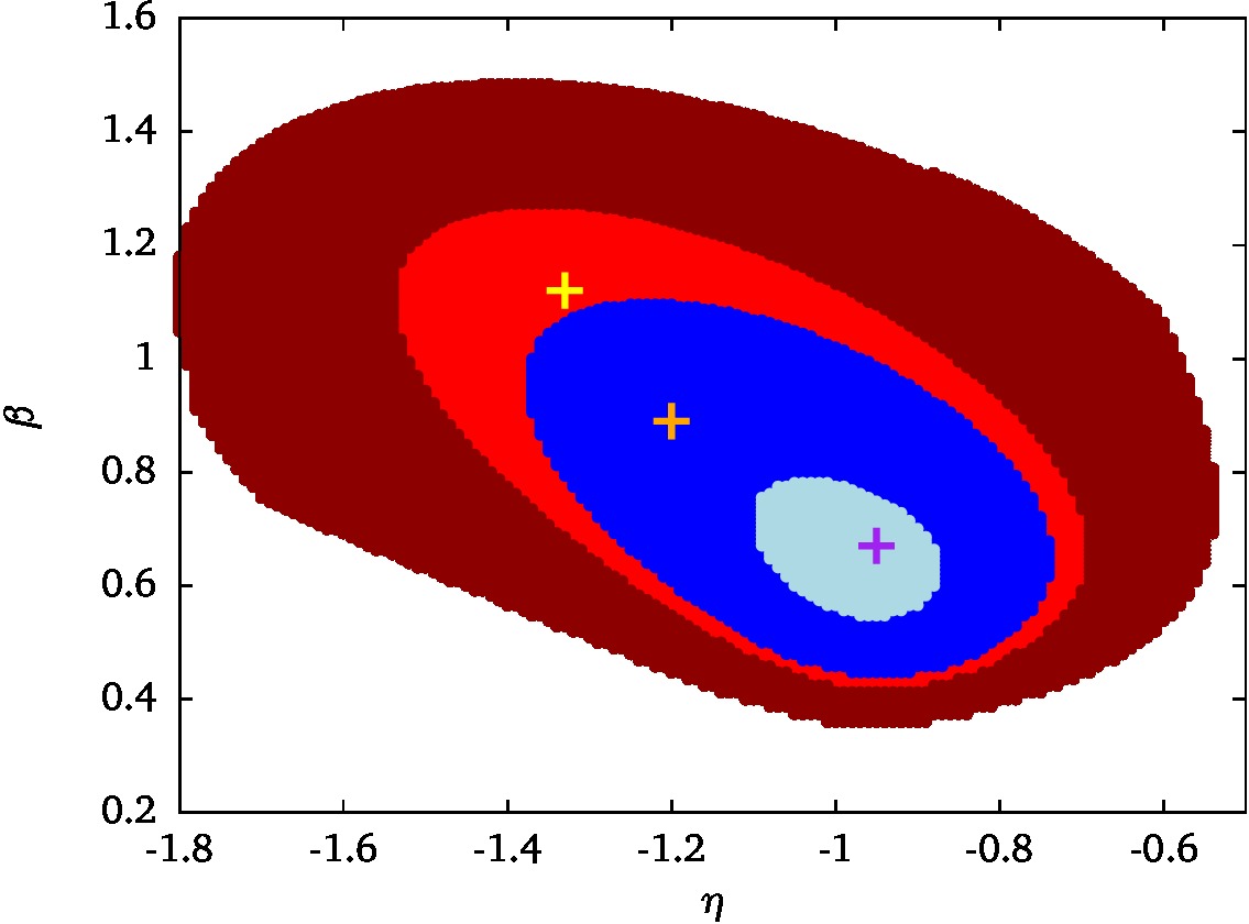
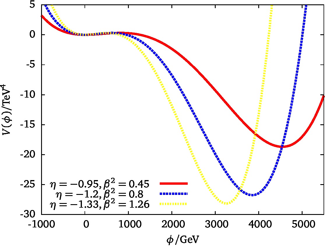
Figure 1: The field configurations for a certain sample point ($\mu=500\,\mathrm{GeV}$, $A_{\mathrm{b}}=A_{\mathrm{t}}=1500\,\mathrm{GeV}$, $\tan\beta=40$ and $M_{\text{SUSY}}=1\,\mathrm{TeV}$), which yields $m_{h^{0}}=126\,\mathrm{GeV}$ with $m_{\tilde{g}}=1.5M_{\text{SUSY}}$ and $m_{A}=800\,\mathrm{GeV}$ but is already excluded by the traditional CCB bound for $A_{\mathrm{b}}$ (the $A_{\mathrm{t}}$-bound is passed) lead to very different conclusions on the stability of the desired vacuum on cosmological scales. While the shape of the potential is qualitatively very much the same over the excluded field space (roughly $\eta\in[-1.8,0.55]$ and $\beta\in[0.13,2.2]$ and the non-standard vev varying within maybe a $1000,\dotsc,2000\,\mathrm{GeV}$ range, the bounce action (shown in contours on the left panel) indicates cosmologically stable and long-lived (blue: $B>400$, light blue: $B>1000$) configuration as well as meta-stable and very short-lived (red: $B<400$, dark red: $B<230$, corresponding to a life-time of less then a second). The crosses on the left-side plot denote positions of the three choices in $\eta$ and $\beta$ shown on the right; the yellow one corresponds to the yellow line, for the others we have $\text{orange}=\text{blue}$ and $\text{purple}=\text{red}$.

 

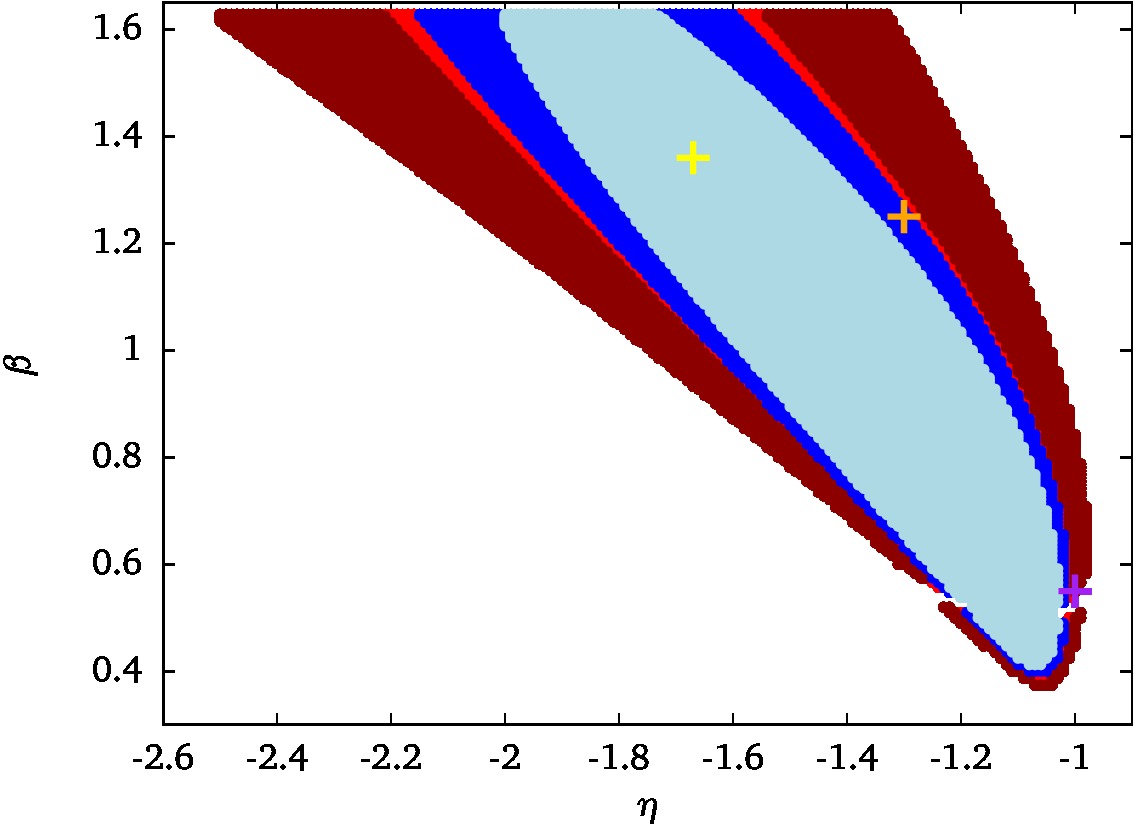
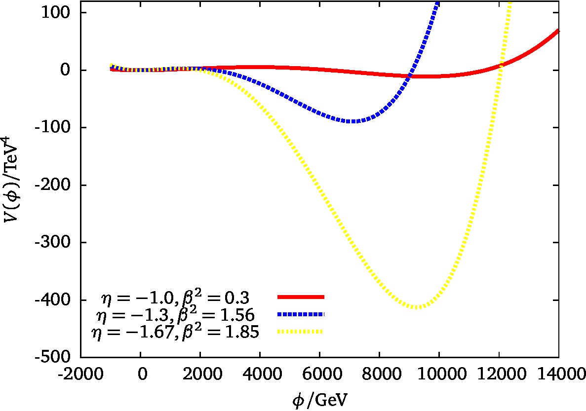
Figure 2: The same as for Fig. 2 but a point which has a long-lived desired vacuum w.r.t. the true vacuum and a too light Higgs of $m_{h^{0}}=113\,\mathrm{GeV}$. We have $A_{\mathrm{t}}=A_{\mathrm{b}}=\mu=500\,\mathrm{GeV}$, $\tan\beta=40$. All other parameters and color coding as in Fig. 2. Here, the global minimum (indicated by the yellow cross in the light blue area) would suggest the desired vacuum to be extremely long-lived. This conclusion may be misleading as there are other configuration with a much shorter tunneling time.

 

To check for metastability, one may be tempted to define the field configuration and the specific ray that shows the deepest non-standard vacuum as the ideal or optimal one. However, as the new vev appears at say $\mathcal{O}(10\,\mathrm{TeV})$ and the barrier in between gets sufficiently high, say $\mathcal{O}(\text{few}\leavevmode\nobreak\ \mathrm{TeV}^{4})$, $B$ is $\gg 400$ in that specific direction as for the point in Fig. 2. However, there are other directions via which the global minimum can be accessed with a much smaller tunneling time. For the sample point of Fig. 1 from above, we show a tomographic view of the scalar potential in the $\tilde{b}$-$h_{\mathrm{u}}$ plane for increasing $\eta=h_{\mathrm{d}}/h_{\mathrm{u}}$ in Fig. 3 and the same potential sliced differently for increasing $\beta=\tilde{b}/h_{\mathrm{u}}$ in the $h_{\mathrm{d}}$-$h_{\mathrm{u}}$ plane in Fig. 4. This is to illustrate that there is no unique choice for some fixed values of $\eta$ and $\beta$ that exclusively show a non-standard vacuum. There are wide regions in field space and all paths should be treated equal to estimate the tunneling rate. The “optimal” direction for the determination of the bounds on the potential parameters (masses, trilinear and quadrilinear couplings) should be rather given by the shortest tunneling time. As recommendation how to deal with any CCB exclusion, we declare each point that fails the condition

$$\mathcal{A}(\eta,\alpha,\beta)^{2}<4\lambda(\eta,\alpha,\beta)M^{2}(\eta,\alpha,\beta)$$

for any specific combination of $\eta$, $\alpha$ and $\beta$ as clearly unstable. An easy (but maybe CPU intensive) way to check this is to scan over a reasonable range, e. g.  $\eta\in[-3,3]$ and $\alpha,\beta\in[0,2]$; with a binning of $0.1$ this procedure should find CCB configurations (since the field space regions are quite extended, even coarser binnings should lead to a trustable result).

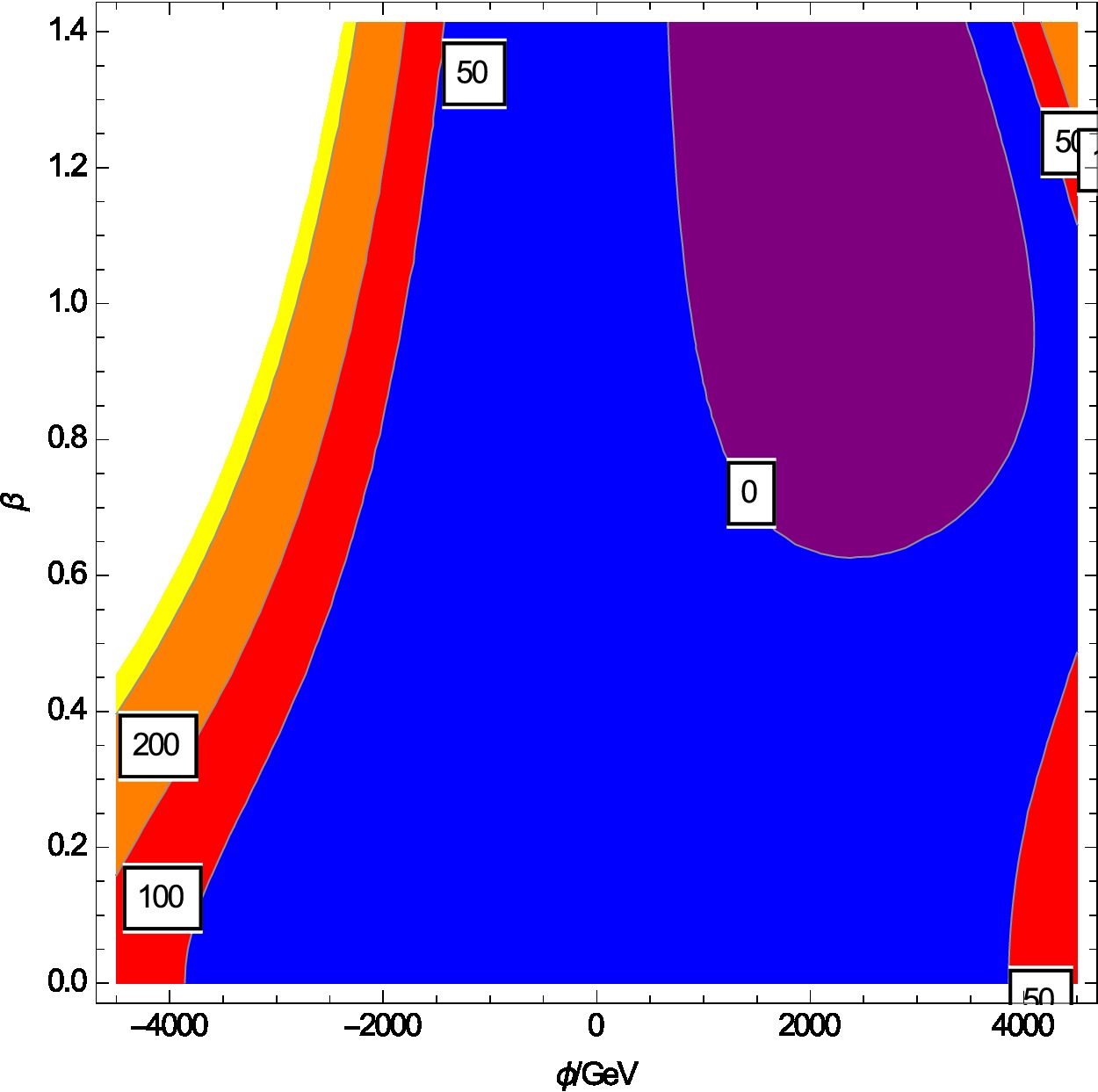
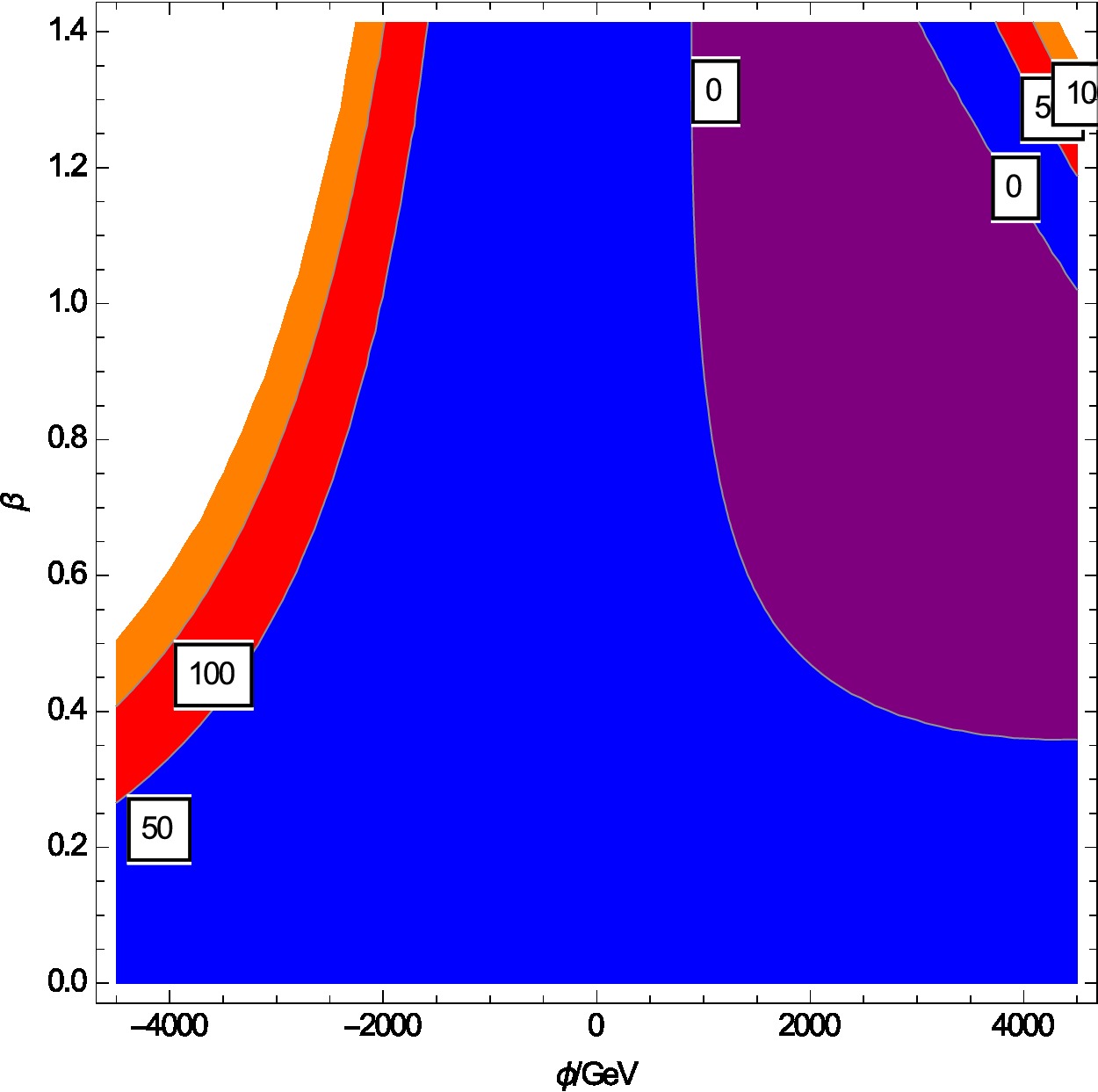
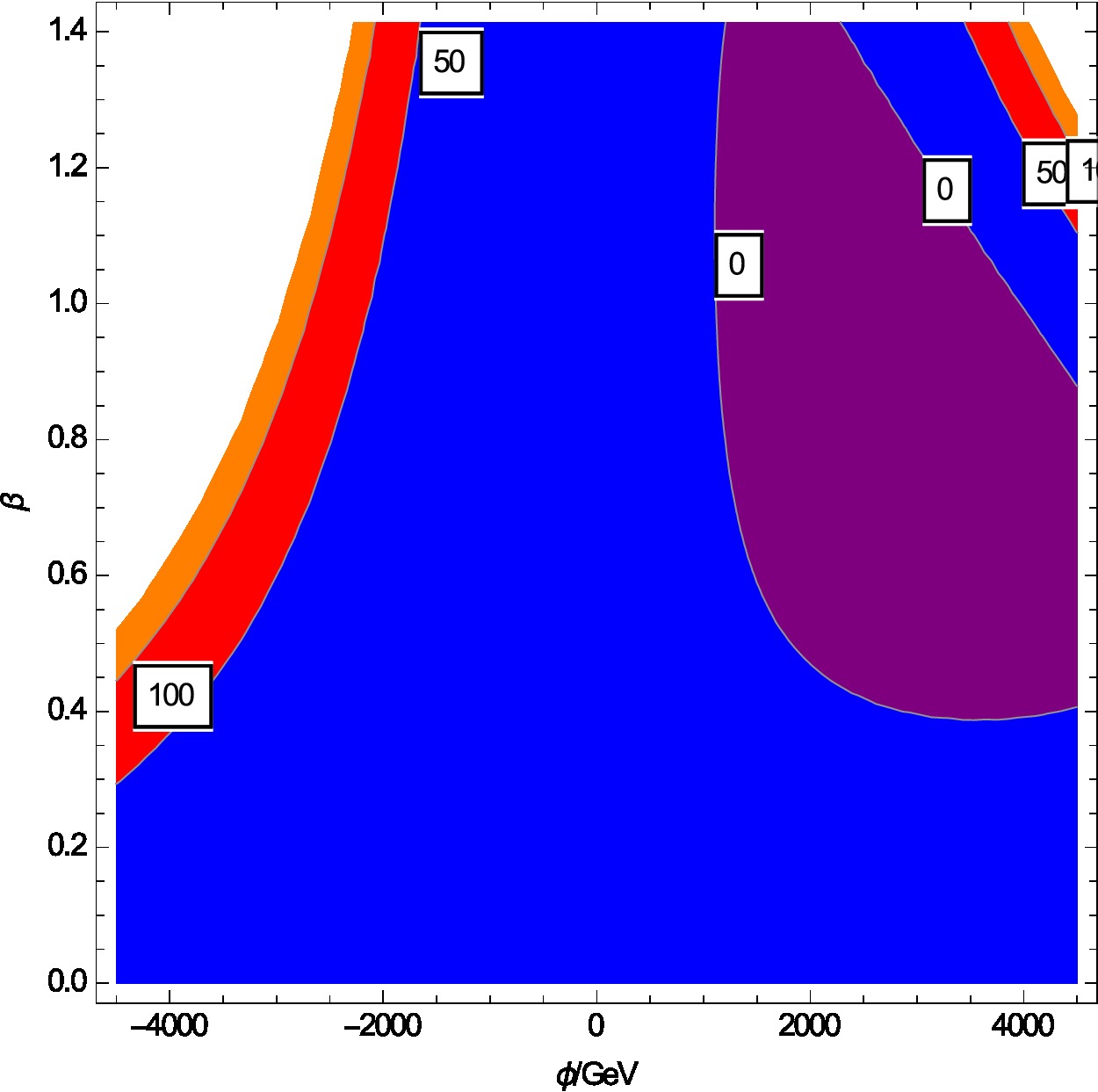
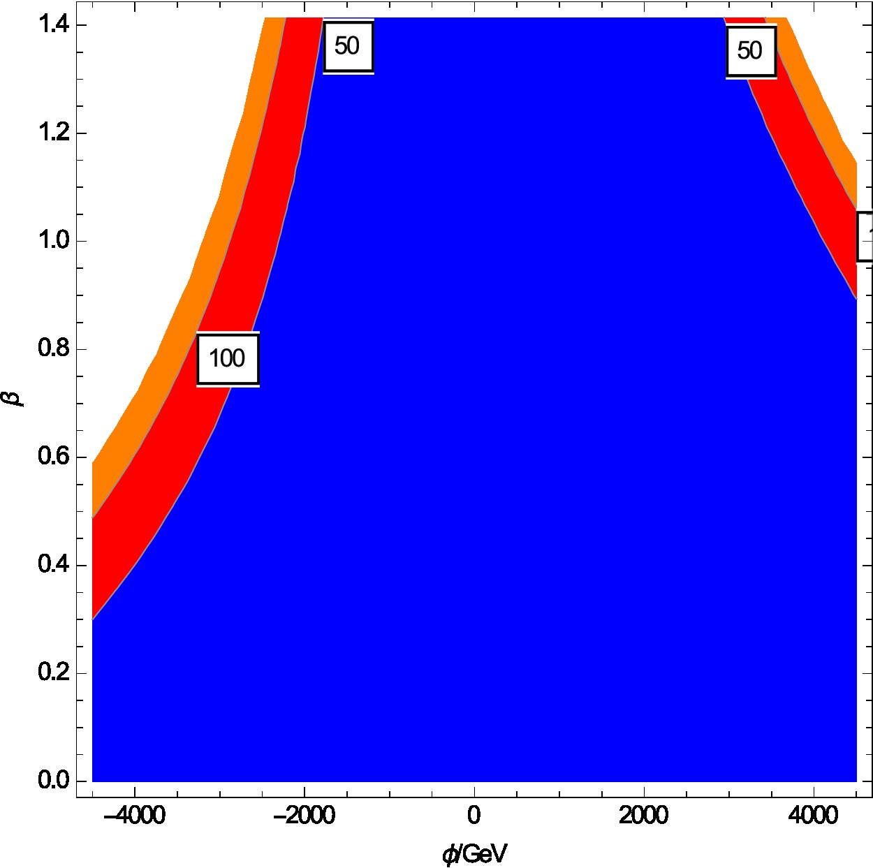
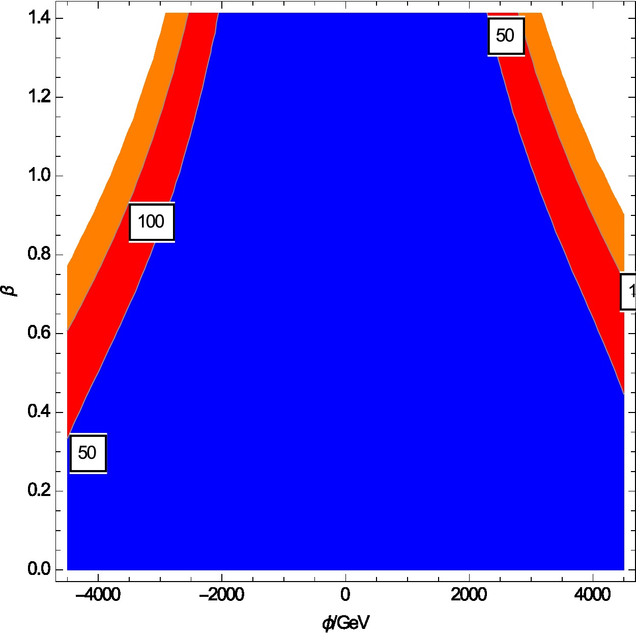
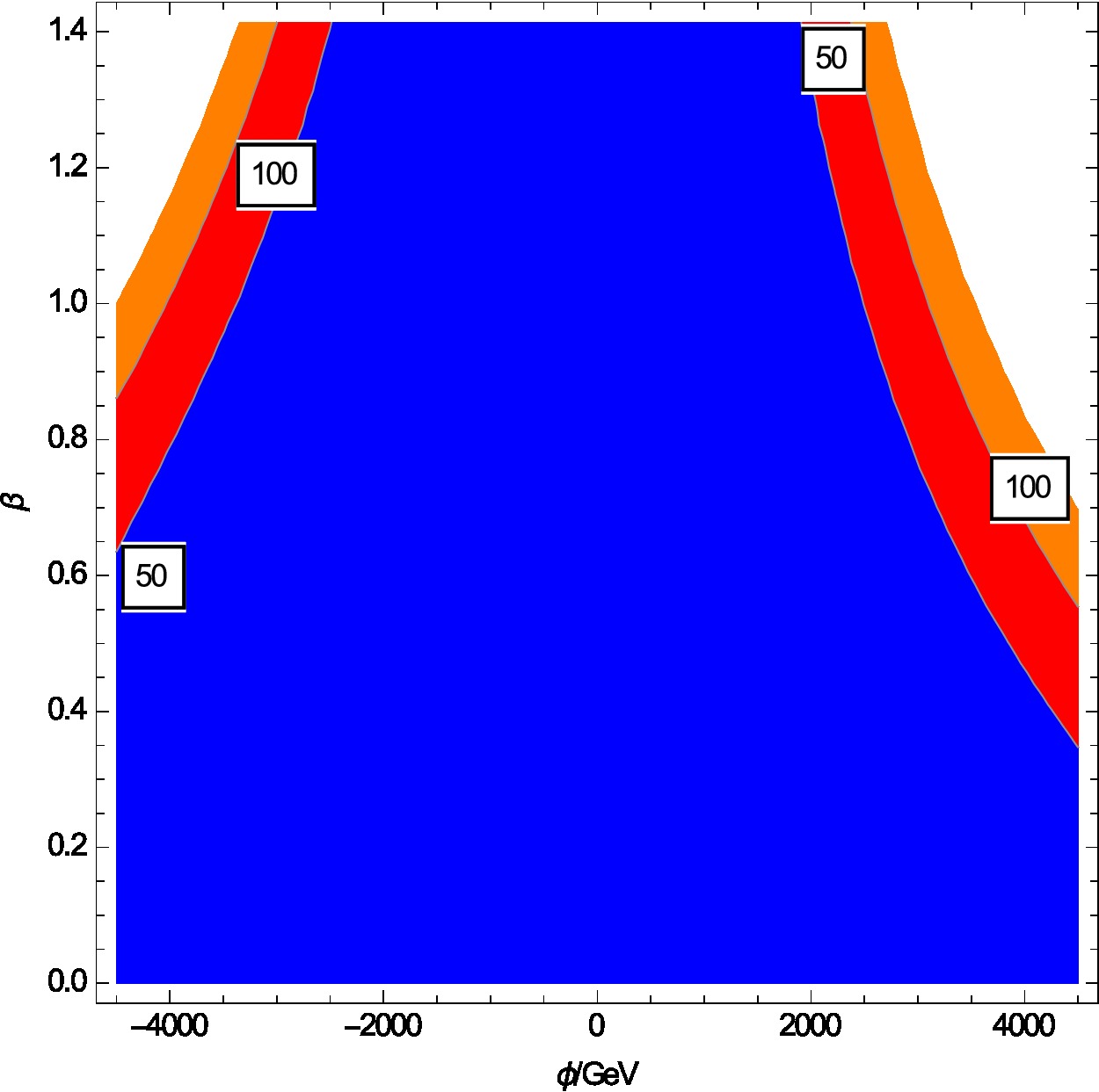
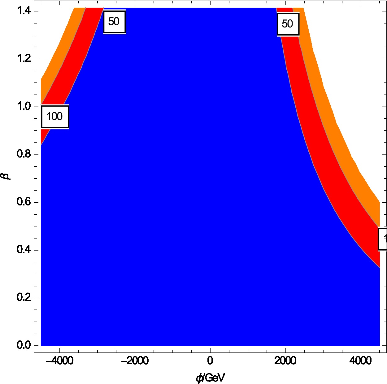
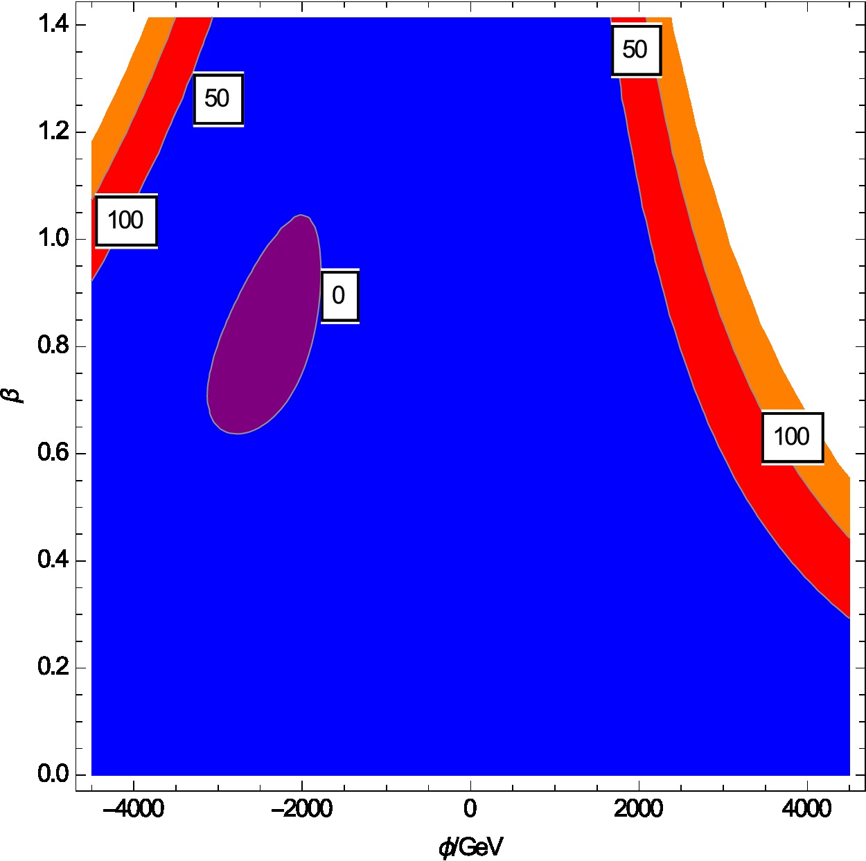
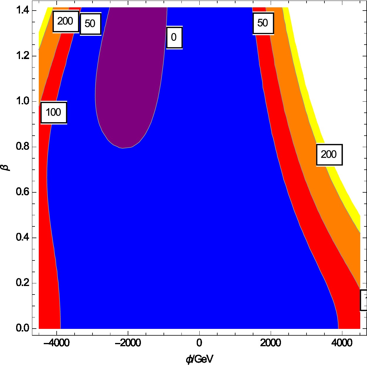
Figure 3: A tomographicly sliced view of the CCB potential in the $\phi=h_{\mathrm{u}}$ and $\tilde{b}=\beta\phi$ direction for $\eta={-1.5,-1.0,-0.8,-0.5,0,0.5,0.8,1.0,1.5}$ (reading single plots from left to right and top to bottom), where $h_{\mathrm{d}}=\eta\phi$. The numbers at the contour lines represent the scaled potential value $V(\phi,\eta,\beta)/\mathrm{TeV}^{4}$ to enhance readability. Negative regions within the $0$-contour indicate the existence of a non-standard true vacuum.

 

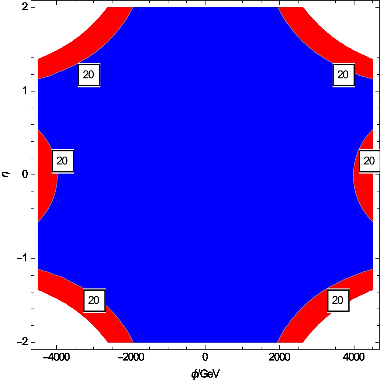
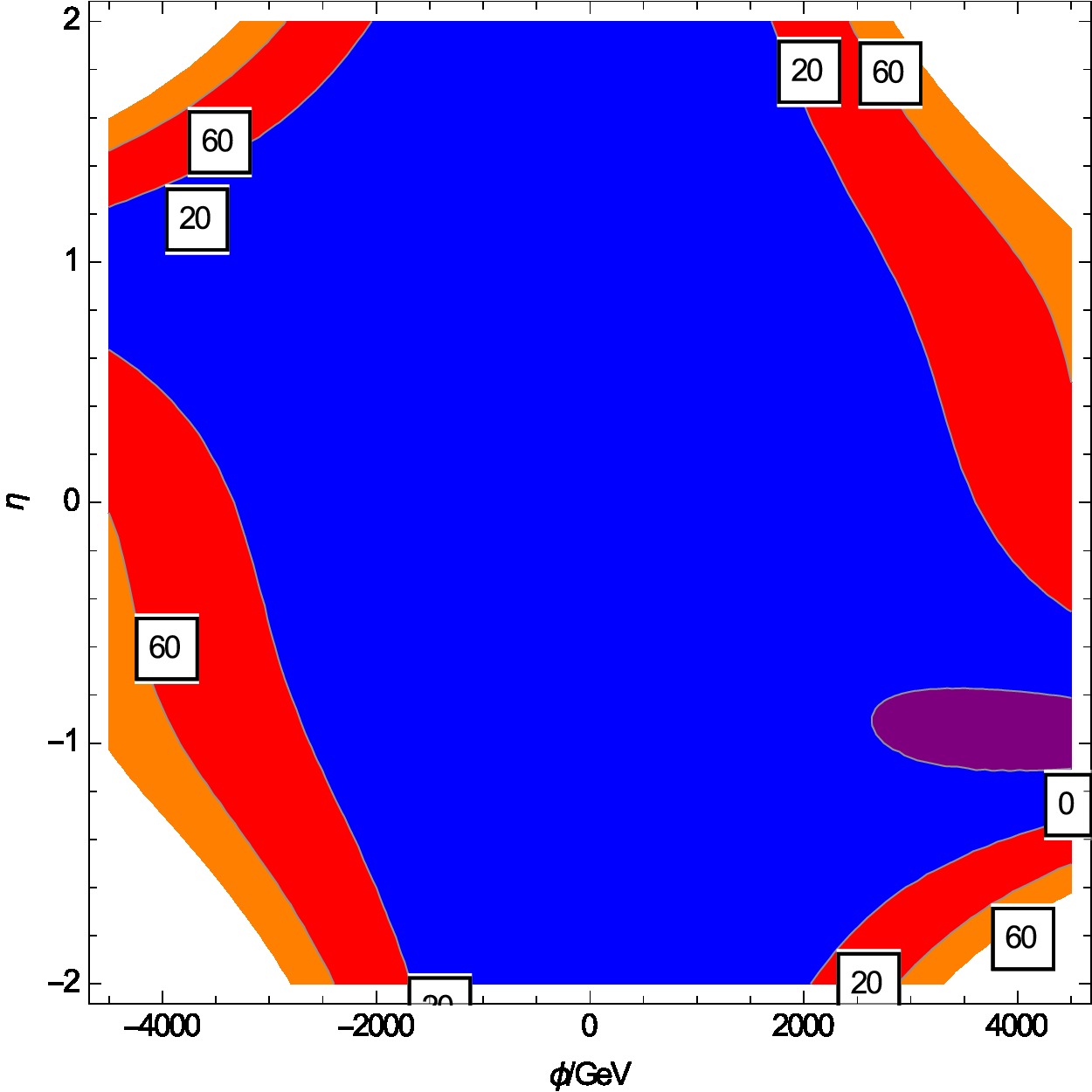
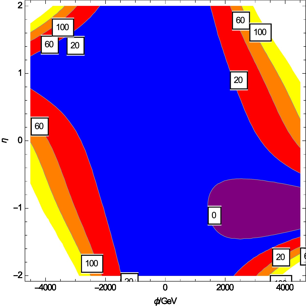
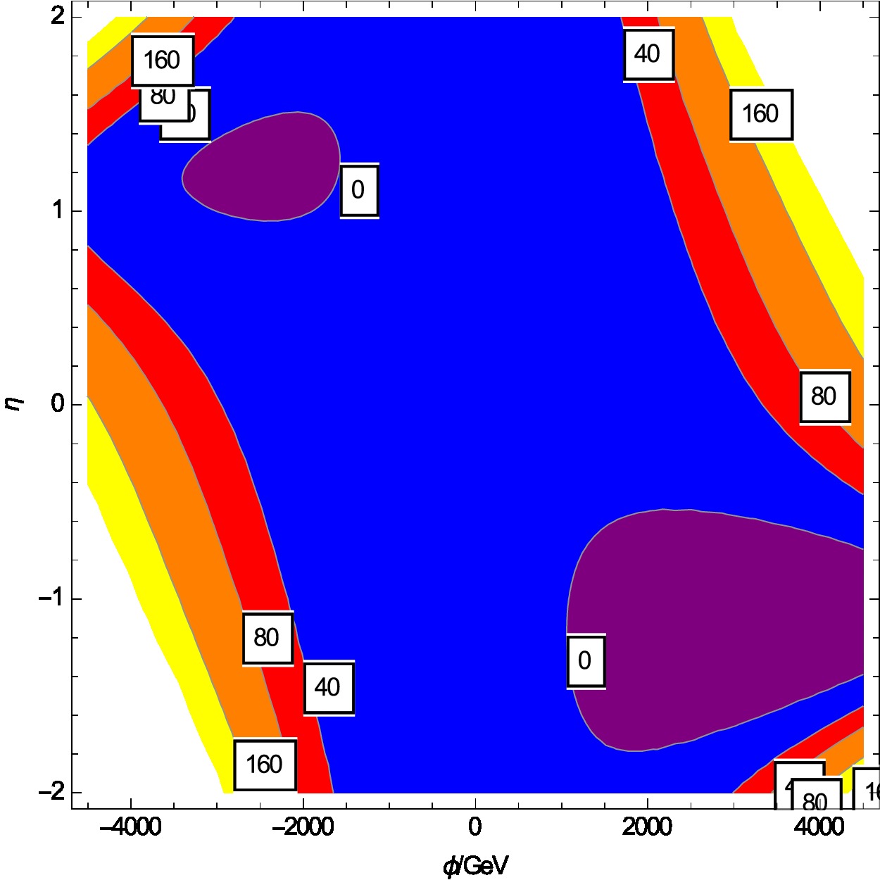
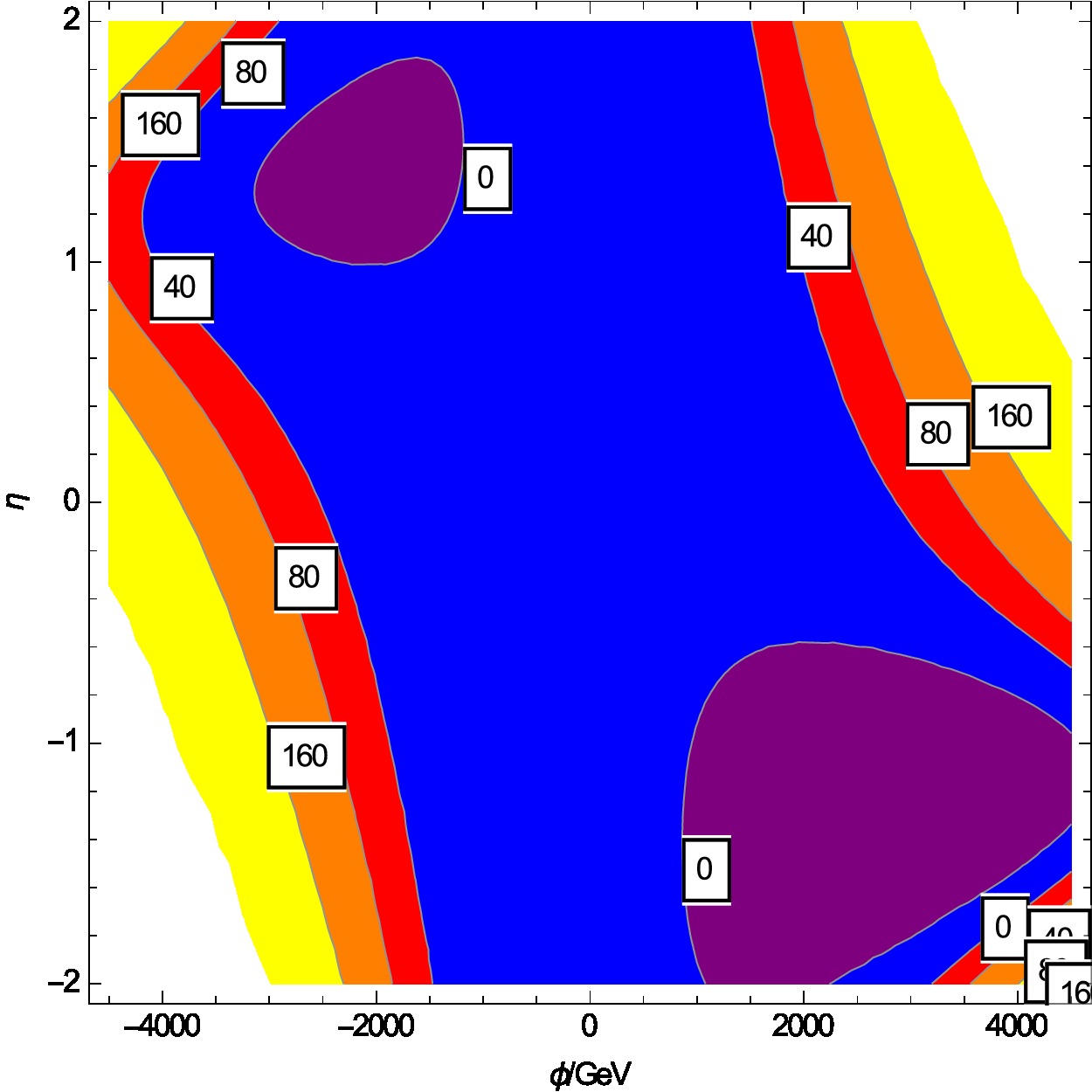
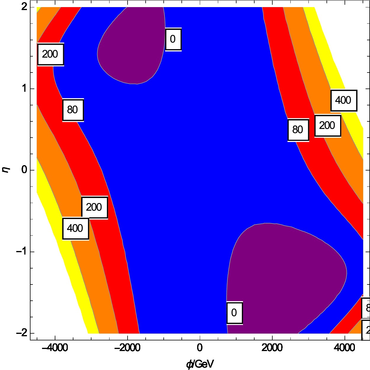
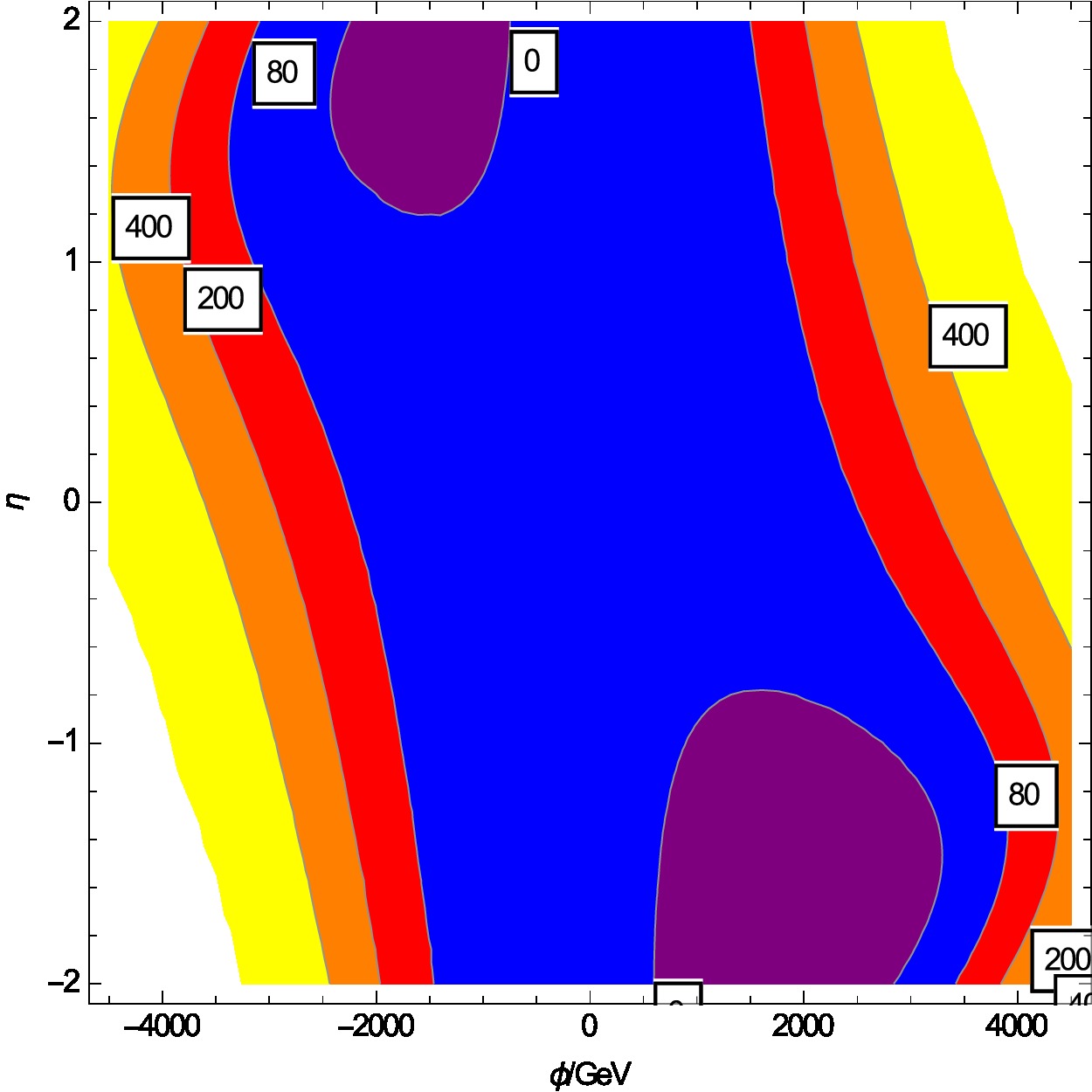
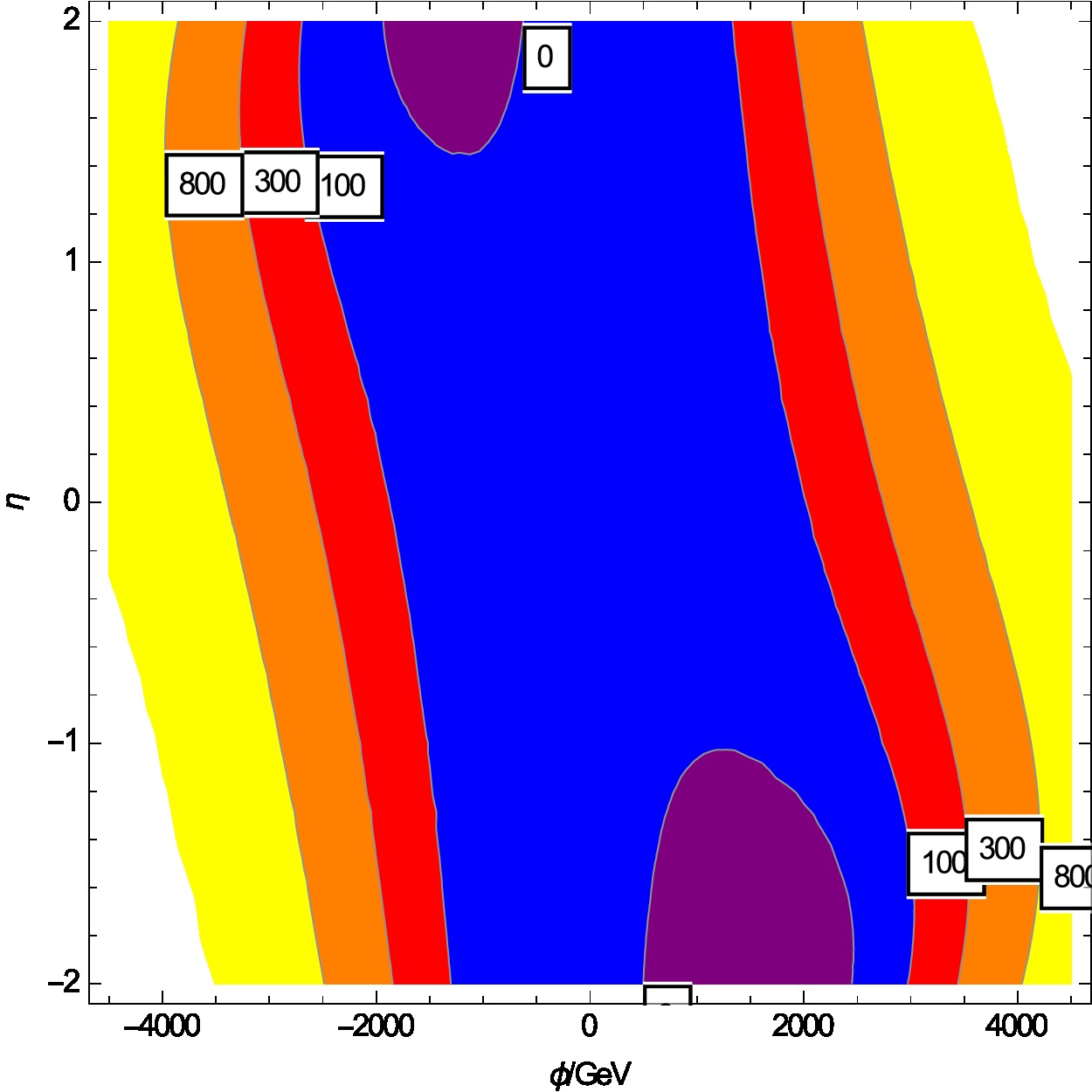
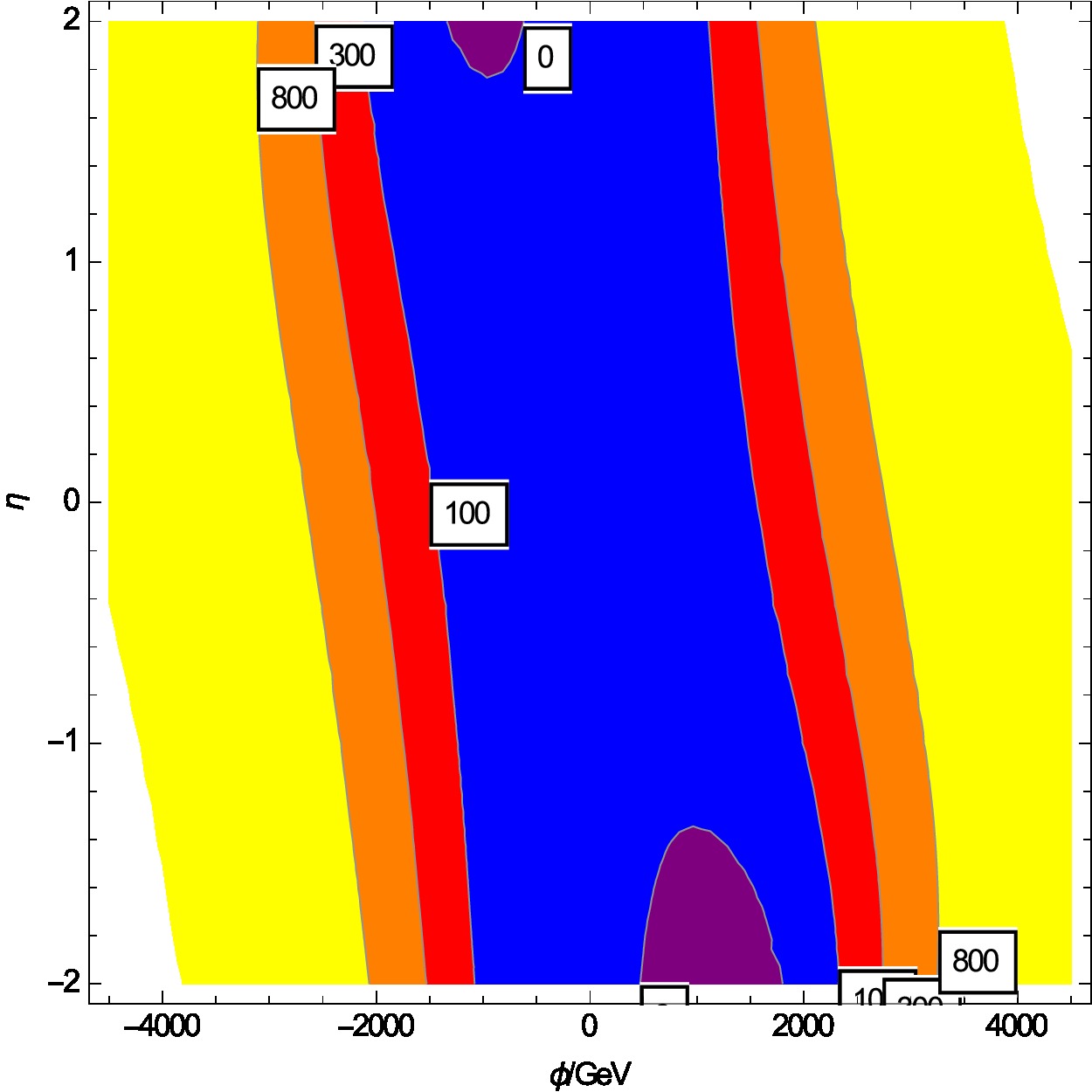
Figure 4: A similar tomographic view as in Fig. 3 in the perpendicular direction with $\eta=h_{\mathrm{d}}/\phi$ on the vertical axis and scanning $\beta=\tilde{b}/\phi$ for $\beta={0,0.4,0.6,0.8,1.0,1.2,1.5,2.0,2.6}$ from left to right and top to bottom with $\phi=h_{\mathrm{u}}$. The existence of up to two non-standard vacua reflects the actually broken reflection symmetry, $\eta\to-\eta$ and $\phi\to-\phi$, as can be seen that there no such exact symmetry.

 

3 Anatomy of Charge and Color Breaking

The main stability condition is given by the unequation

$$M^{2}(\eta,\alpha,\beta)>\frac{A(\eta,\alpha,\beta)^{2}}{4\lambda(\eta,\alpha,\beta)},$$ (19)

depending on the field misalignments, as well as on all relevant model parameters. We distinguish between parameters in configuration space that independently of the model parameters can lead to instable configurations, such as $\alpha$, $\beta$ and $\eta$—and the model parameters that change the shape of the scalar potential as whole object (such as the soft masses, the trilinear couplings $A_{\mathrm{t}}$ and $A_{\mathrm{b}}$ as well as the $\mu$-parameter). Furthermore, we request the parameters of the one-loop Higgs potential (i. e. the genuine type-II 2HDM of the MSSM) to allow for spontaneous electroweak breaking with the correct vevs. The ratio of the standard $v_{\mathrm{u}}/v_{\mathrm{d}}$ is what we call $\tan\beta$, obeying $v_{\mathrm{d}}^{2}+v_{\mathrm{u}}^{2}=v^{2}=(246\;\mathrm{GeV})^{2}$. Note that finally, the “true” $\tan\beta$ will be given by $1/\eta$. We neither keep $\tan\beta$ fixed in a sense that the true vacuum has to respect this relation, nor do we infer that from an original $\tan\beta>1$ the ratio $\langle h_{\mathrm{u}}\rangle/\langle h_{\mathrm{d}}\rangle$ has to have the same property. What we actually find is that for most configurations the true vacuum seems to have $\langle h_{\mathrm{d}}\rangle>\langle h_{\mathrm{u}}\rangle$ and the CCB vev typically shows $\langle\tilde{q}\rangle\gtrsim 0.7\langle h_{\mathrm{u}}\rangle$. Unfortunately, for the bounds deduced numerically by attempting to find the global minimum of parameter points violating (19), no expression of the scaling parameters $\alpha$, $\beta$ and $\eta$ can be found in terms of the relevant potential parameters although they crucially depend on the MSSM parameter point. The ideal solution would be an exclusion of the form (19) with $\eta$, $\alpha$ and $\beta$ given in terms of the model parameters. Similar attempts have been achieved by [27] where one trilinear operator at a time was considered only. For four operators this appears to be impossible.

For the numerical analysis in the following, we consider a very phenomenological version of the MSSM with all SUSY breaking parameters defined at the low (SUSY) scale without referring to any high-scale unified scenario. As the developing CCB minima typically also show up around the same low scale, we ignore any effects from the renormalization group as the corresponding logarithms are small and only have a mild impact on the shape of the potential (see e. g.  [34] and the reference therein to [72]). For the qualitative discussion this point is irrelevant anyway. Quantitatively, if desired, parameters at the relevant scale can be employed as input values for the analytical bounds.

We determine the soft SUSY breaking Higgs masses $m_{H_{\mathrm{u}}}^{2}$ and $m_{H_{\mathrm{d}}}^{2}$ requiring electroweak symmetry breaking via the conditions $\partial V_{1}/\partial h_{\mathrm{u}}\big{|}_{h_{\mathrm{u}}=v_{\mathrm{u}},h_{\mathrm{d}}=v_{\mathrm{d}}}=0$ and $\partial V_{1}/\partial h_{\mathrm{d}}\big{|}_{h_{\mathrm{u}}=v_{\mathrm{u}},h_{\mathrm{d}}=v_{\mathrm{d}}}=0$ with the one-loop Higgs potential $V_{1}$ [42]. The bilinear soft breaking term is related to the pseudoscalar mass at tree-level via $B_{\mu}=m_{A}^{2}\sin\beta\cos\beta$. Our free parameters are the ratio of the two Higgs vevs at tree-level, $\tan\beta=v_{\mathrm{u}}/v_{\mathrm{d}}$, the soft squark masses, which we for simplicity set to ${\tilde{m}}_{Q}^{2}={\tilde{m}}_{t}^{2}={\tilde{m}}_{b}^{2}=M_{\text{SUSY}}^{2}$, and the superpotential parameter $\mu$ as well as the soft breaking trilinear Higgs–squark couplings $A_{\mathrm{t}}$ and $A_{\mathrm{b}}$. The gaugino masses $M_{1},M_{2}$ and $M_{3}$ enter only indirectly and play a less crucial role, where the gluino mass $M_{3}$ can be more important for the threshold effects on the bottom Yukawa coupling and in the two-loop light Higgs mass as provided by FeynHiggs. If nothing else is stated, we set $M_{1}=M_{2}=M_{\text{SUSY}}=1\,\mathrm{TeV}$ and $M_{3}=1.5M_{\text{SUSY}}$.

Including bottom Yukawa effects in the analysis of CCB minima has not been done to great extend in the literature, as $y_{\mathrm{b}}$ usually is neglected because of its smallness. However, for large $\tan\beta$ and certain other regions in parameter space this cannot be done anymore. Especially the $\Delta_{b}$ resummation for the bottom quark mass effectively changes the bottom Yukawa coupling dramatically for such regions. While $y_{\mathrm{b}}$ gets lowered compared to $m_{\mathrm{b}}/v_{\mathrm{d}}$ for large $\tan\beta$, it grows severely for negative $\mu$ as can be seen from the expressions and even runs into a non-perturbative region (what is a well-known behavior). The reduction at large $\tan\beta$ and small but positive $\mu$ keeps this window open in the following analysis. We include the dominant contributions to $\Delta_{b}$ from the gluino and the higgsino loop [73, 74, 75, 76],

$$\Delta_{b}^{\text{gluino}} =\frac{2\alpha_{s}}{3\pi}\mu M_{\tilde{G}}\tan\beta C_{0}(\tilde{m}_{\tilde{b}_{1}},\tilde{m}_{\tilde{b}_{2}},M_{\tilde{G}}),$$ (20a)

$$\Delta_{b}^{\text{higgsino}} =\frac{y_{\mathrm{t}}^{2}}{16\pi^{2}}\mu A_{\mathrm{t}}\tan\beta C_{0}(\tilde{m}_{\tilde{t}_{1}},\tilde{m}_{\tilde{t}_{2}},\mu),$$ (20b)

and get the corrected bottom Yukawa coupling with $\Delta_{b}=\Delta_{b}^{\text{gluino}}+\Delta_{b}^{\text{higgsino}}$ as

$$y_{\mathrm{b}}=\frac{m_{\mathrm{b}}}{v_{\mathrm{d}}(1+\Delta_{b})}.$$ (21)

Another remark is inevitable on the relevance of the parameters in the discussion. Usually, when MSSM effects on the Higgs mass are discussed, the “stop mixing parameter” $X_{t}=A_{\mathrm{t}}/y_{\mathrm{t}}-\mu\cot\beta$ is used to measure the strength of the corrections rescaled with the SUSY scale, $X_{t}/M_{\text{SUSY}}$. In the maximal mixing scenario, this parameter is set to a large value, $X_{t}=\sqrt{6}M_{\text{SUSY}}$ what appears to be in trouble with the exclusions presented here. Although it would be desired to directly impose constraints on $X_{t}$, we are unable to do so because the two independent Higgs vevs $v_{\mathrm{d}}$ and $v_{\mathrm{u}}$ have to be treated as dynamical variables and $\tan\beta$ cannot be kept fixed. Doing so would lead to wrong conclusions. However, we can translate the final exclusions we found to an effective exclusion on $X_{t}$ where $\tan\beta=v_{\mathrm{u}}/v_{\mathrm{d}}$ gives the ratio of the two Higgs vevs in the desired electroweak state. This is especially important in connection to the importance of $X_{t}$ for the light Higgs mass.

In comparison with earlier work on the vacuum stability issue in the MSSM, we are now able to exclude a wider region of parameter space which gets accessed when both stop and sbottom vevs and non-standard values for the two Higgs doublets are considered. Non-standard in this respect means $\langle h_{\mathrm{u}}\rangle\neq v_{\mathrm{u}}=v\sin\beta$ and $\langle h_{\mathrm{d}}\rangle\neq v_{\mathrm{d}}=v\cos\beta$. Excluded regions in the $\mu$-$\tan\beta$ plane have been derived from an analysis of the one-loop Higgs potential in the MSSM, where loop effects of third generation sfermions have been included [42]. An additional minimum seems to appear at a larger field value $h_{\mathrm{u}}$ which is driven by the $\mu$-term and therefore the requirement is that this non-standard (apparently charge and color conserving!) vev does not lead to a minimal value of the potential that is lower than at the electroweak vev. Actually, this behavior is an artifact of neglecting colored directions in the potential already at the tree-level leading to an imaginary part in the example of Ref. [42] that was not understood (and therefore just ignored). As this imaginary part is related to a tachyonic sbottom mass at the new vev, this indicates a CCB global minimum, where the “one-loop global minimum” is rather a saddle point of the potential in the Higgs–sbottom field configuration. For the same configuration (basically $h_{\mathrm{d}}=0$ and $\tilde{b}=h_{\mathrm{u}}$) the shape of the exclusion is very much the same but a bit tighter and shown in the upper left plot of Fig. 5. The choice of $h_{\mathrm{d}}=0$ basically follows from the consideration that if $\langle h_{\mathrm{d}}\rangle=v_{\mathrm{d}}$ kept fixed, this value can be neglected for large $\tan\beta$ with respect to the much larger $\langle h_{\mathrm{u}}\rangle>v_{\mathrm{u}}$. However, this choice (as well as $\tilde{b}\sim h_{\mathrm{u}}$) does not resemble the true behavior of the potential as can be seen, when both $h_{\mathrm{d}}$ and $\tilde{b}$ are treated as independent dynamical variables as described above. If one commits to the genuine $D$-flat direction only (say $|h_{\mathrm{d}}|^{2}=|h_{\mathrm{u}}|^{2}+|\tilde{b}|^{2}$), similarly wrong exclusions (conclusions?) can be drawn. The comparison of these two choices has been elaborated in [43] together with the corresponding analytic bound Uneqs. (13) and (14). The combined exclusion limit interpolates between the two and is shown in the upper right plot of Fig. 5. Again, the artificial constraint $\tilde{t}=0$ leads to weaker exclusions than under a non-vanishing stop vev. This behavior finally is shown in the lower left plot of Fig. 5 and excludes large parts of the $\mu$-$\tan\beta$ plane. So far, we also have kept the trilinear soft SUSY breaking sbottom parameter $A_{\mathrm{b}}$ to zero and employed a large but moderate $A_{\mathrm{t}}=-1500\,\mathrm{GeV}$ (the negative sign was chosen to enhance the sbottom-vev bound related to $y_{\mathrm{b}}$). As a non-vanishing $A_{\mathrm{b}}$ drives the formation of vacua with $\langle\tilde{b}\rangle\neq 0$ and similarly $\langle h_{\mathrm{d}}\rangle\gg v_{\mathrm{d}}$, we close the remaining allowed parameter space to values of $\tan\beta\gtrsim 40$ and $\mu\lesssim 700\,\mathrm{GeV}$ (in a world with ${\tilde{m}}_{Q}={\tilde{m}}_{t}={\tilde{m}}_{b}=M_{\text{SUSY}}=1\,\mathrm{TeV}$ and $m_{A}=800\,\mathrm{GeV}$ as the relevant further input parameters).

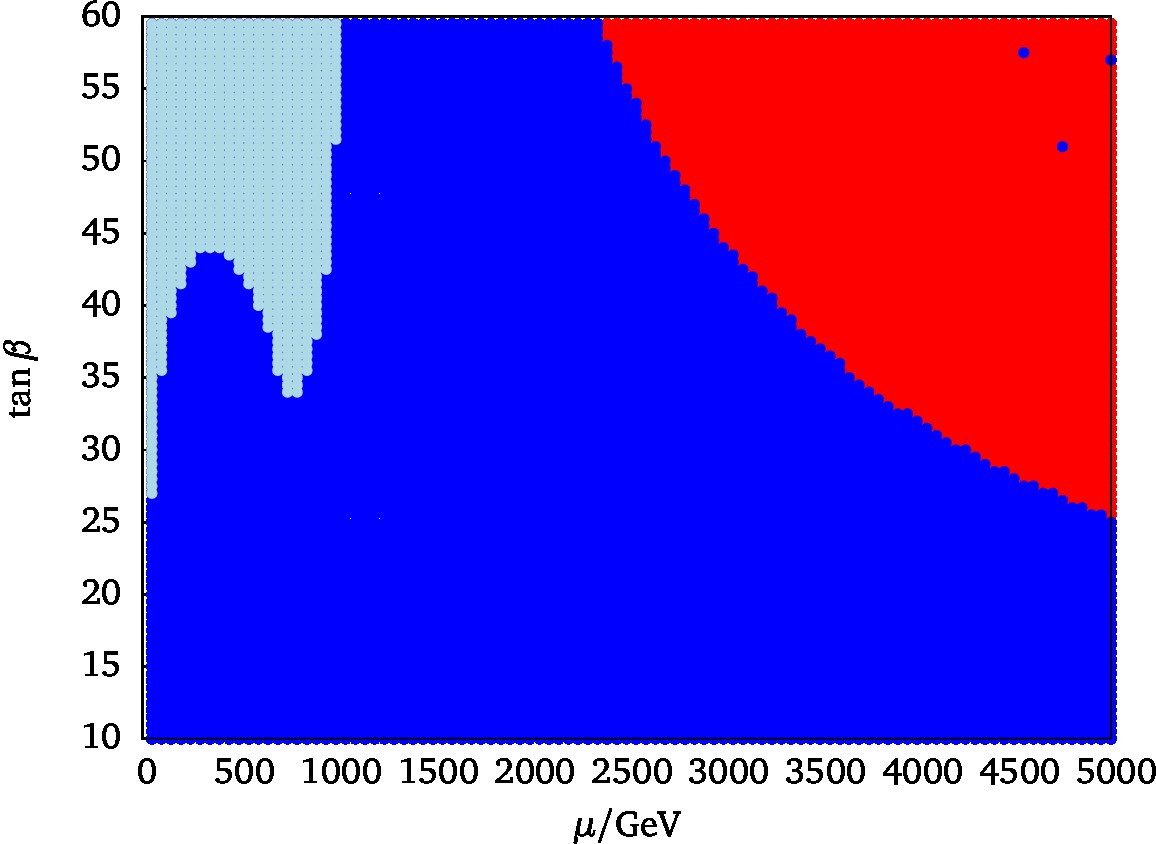
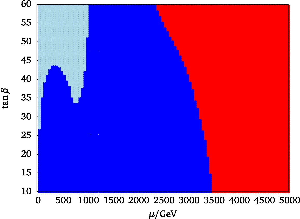
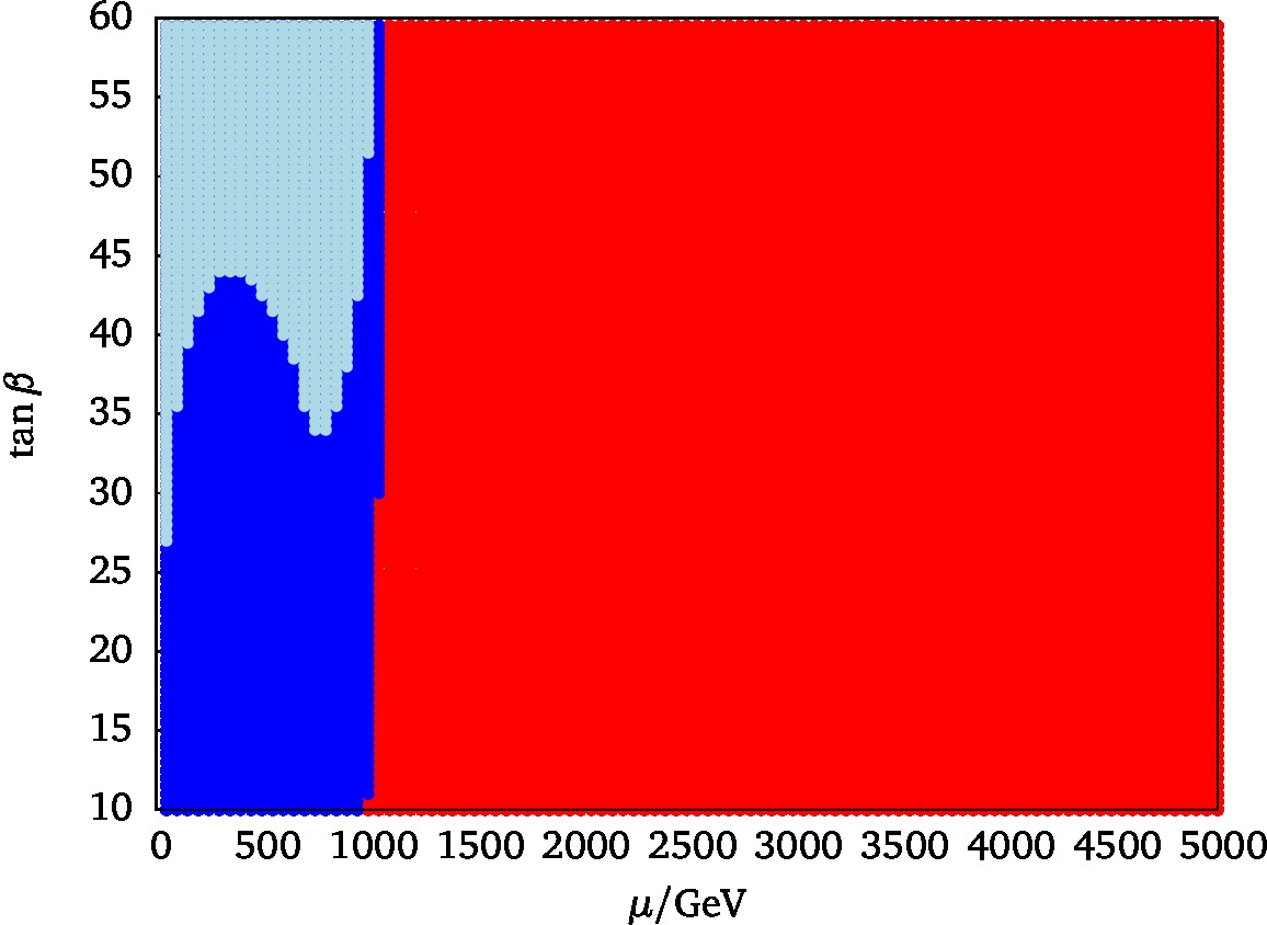
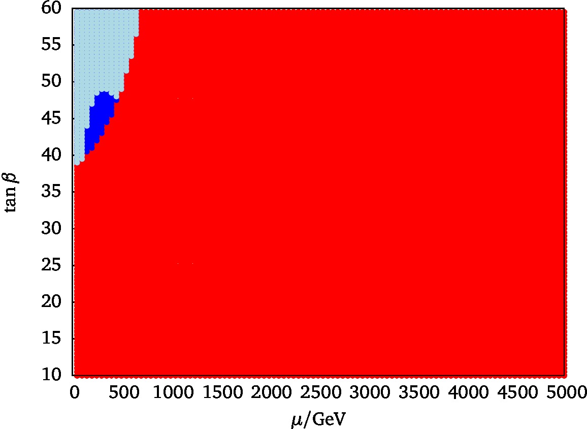
Figure 5: Growing exclusion limits if more vevs are allowed; red points are excluded by vacuum stability, blue points are still allowed. The light blue points indicate a light Higgs mass within $125\pm 1\,\mathrm{GeV}$ (FeynHiggs with a gluino mass at $3M_{\text{SUSY}}$). All plots have $A_{\mathrm{t}}=-1500\,\mathrm{GeV}$ and $M_{\text{SUSY}}=1\,\mathrm{TeV}$ for comparison with previous works. Top left: similar configuration as in [42, 43] with no stop and $h_{\mathrm{d}}$ vevs; top right: including also $h_{\mathrm{d}}\neq 0$, where the exclusion is now interpolating between the two scenarios of [43] and is a bit stronger (as not necessarily $|h_{\mathrm{d}}|^{2}=|h_{\mathrm{u}}|^{2}+|\tilde{b}|^{2}$ is fixed). Down left: including all field directions discussed in this paper, as in the upper row we kept $A_{\mathrm{b}}=0$; down right: now switching on $A_{\mathrm{b}}=A_{\mathrm{t}}$, nearly the complete area seems to be excluded. To compare with the usual (p)MSSM literature, we have to rescale the $A$-terms $A_{\mathrm{t}}\to A_{\mathrm{t}}/y_{\mathrm{t}}$ and $A_{\mathrm{b}}\to A_{\mathrm{b}}/y_{\mathrm{b}}$. In this area, $y_{\mathrm{b}}$ ranges from $\sim 0.12$ to $\sim 0.8$ and gets large in the upper left corner of the $\mu$-$\tan\beta$ plane including the $\Delta_{b}$ resummation but less large than $m_{\mathrm{b}}/v_{\mathrm{d}}$ (which seems to rescue this corner once $A_{\mathrm{b}}$ is switched on).

 

How much is the interplay of stop and sbottom vevs? The exclusion from stop vevs only has a rather circular shape in the $\mu$-$A_{\mathrm{t}}$ plane, illustrated in Fig.6. This shape does not change much with $\tan\beta$ as long as $A_{\mathrm{b}}$ is switched off. In the upper left corner, we show exactly this for $\tan\beta=40$ and $A_{\mathrm{b}}=0$. For the purposes of Figs. 5 and 6, we relied on our own determination of the Higgs potential parameters (basically $m_{H_{\mathrm{u}}}^{2}$ and $m_{H_{\mathrm{d}}}^{2}$ to have the correct $v_{\mathrm{d},\mathrm{u}}$ in presence of the one-loop corrected potential). Comparison of public codes doing the same (SPheno [77, 78], softsusy [79] and SuSpect [80] with the convenient Mathematica interface SLAM [81]) shows very similar shapes, where the border lines get less sharp due to several effects we do not have under control. For aesthetic reasons, we show the (slightly wrong but nicer) plots determined with our own algorithm. The color coding in Fig. 6 shows allowed regions in blue, excluded by stop vevs in red and sbottom vev appearing in orange. As can be seen by turning on $A_{\mathrm{b}}$, a larger portion of the previously allowed parameter space is excluded. The allowed parameter space for $m_{h^{0}}$ within a $1\,\mathrm{GeV}$ interval around $125\,\mathrm{GeV}$ is shown in light blue.

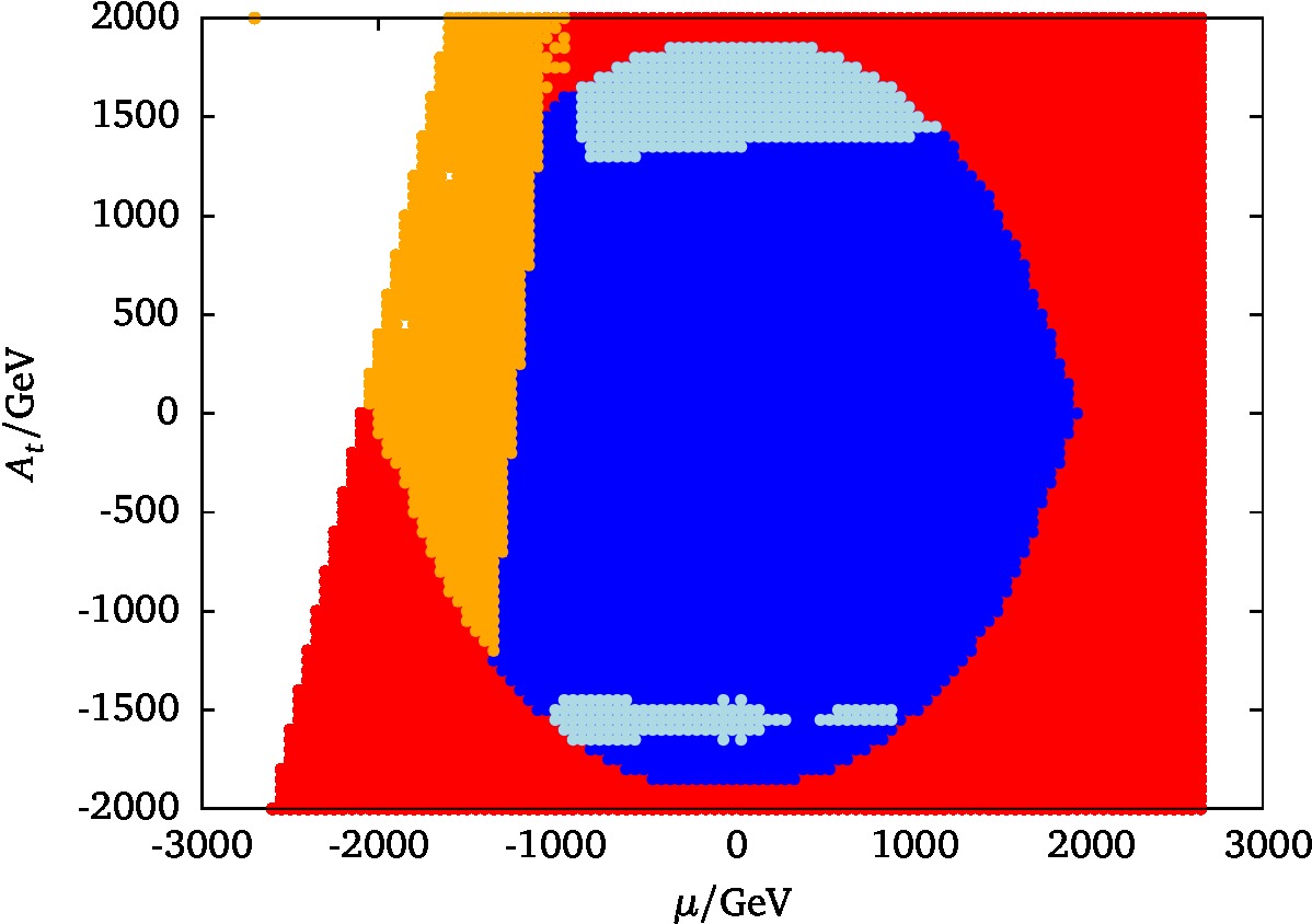
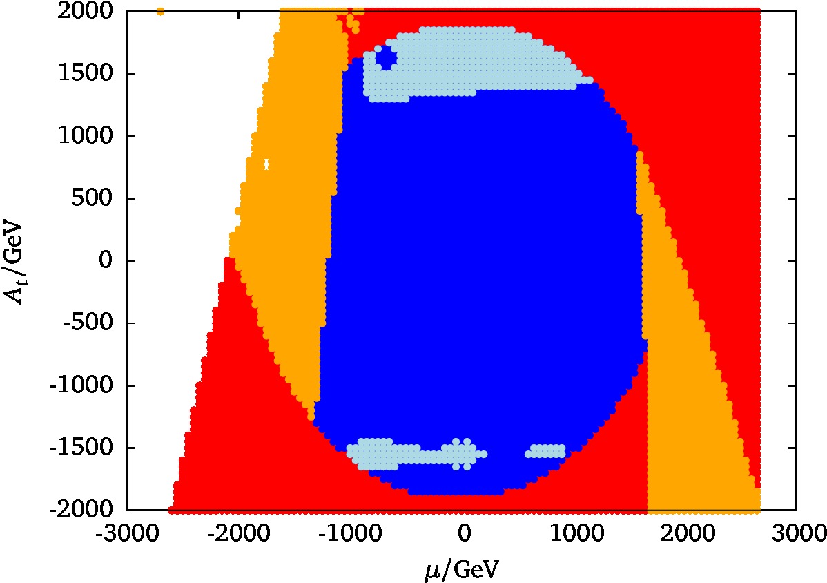
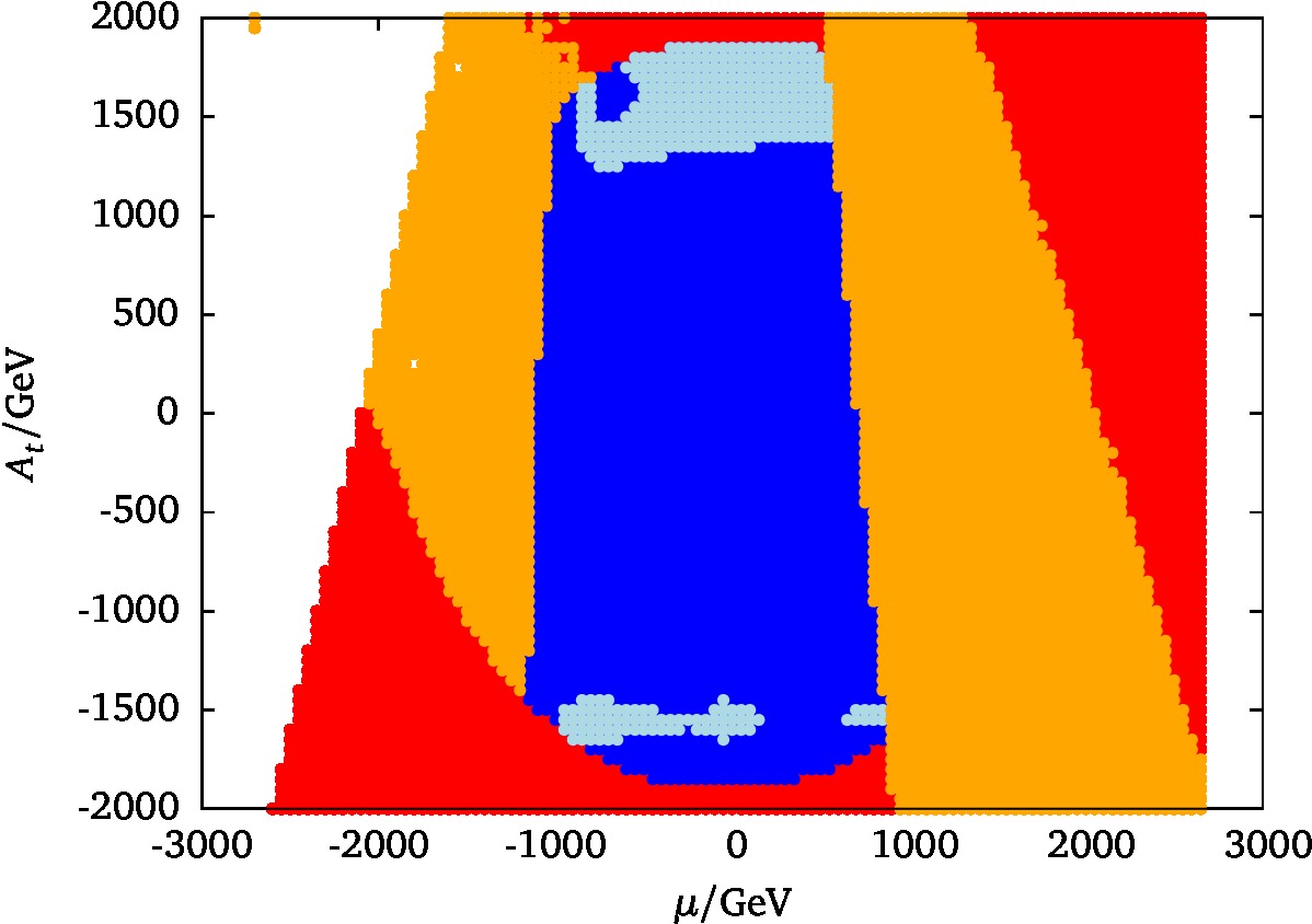
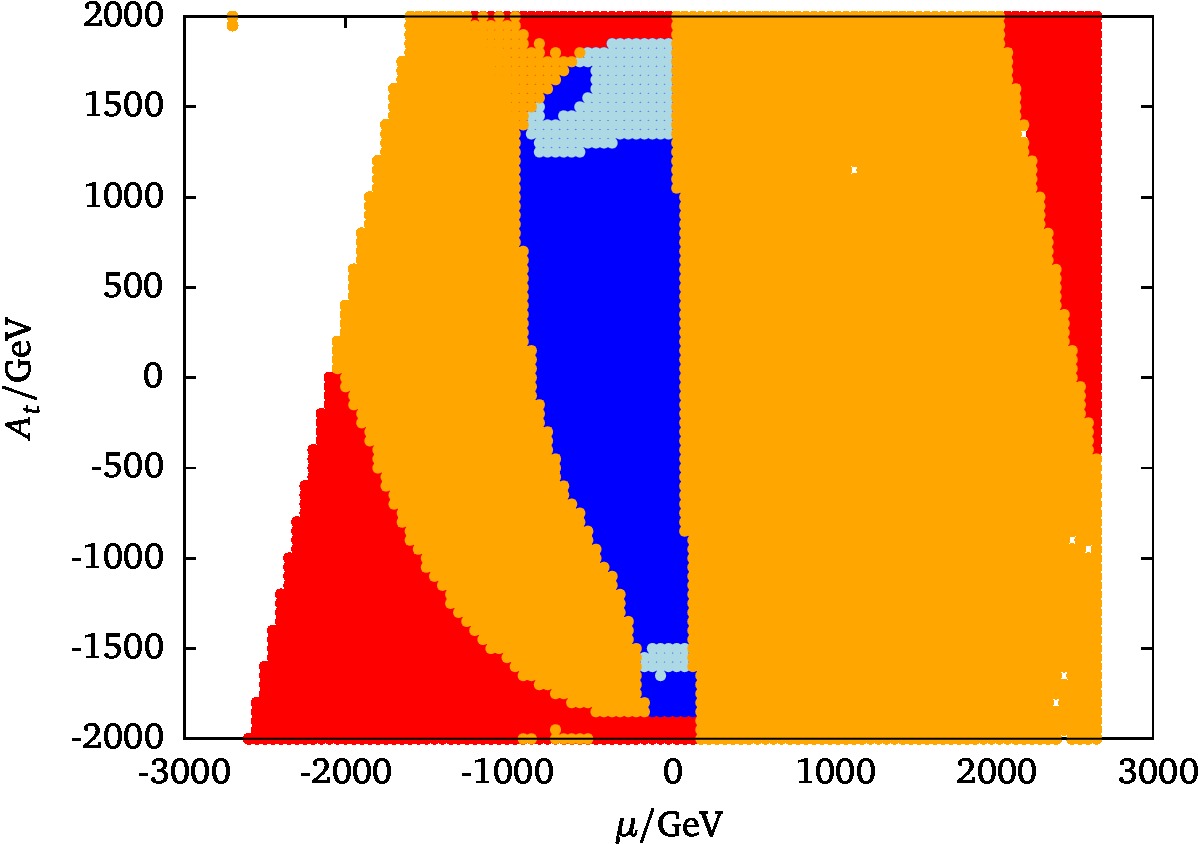
Figure 6: We show exclusion limits from the formation of non-standard vacua in the $A_{\mathrm{t}}$-$\mu$ plane. The central blue area appears to be allowed, where the red and orange regions are excluded by the existence of stop and sbottom vevs, respectively. Light blue points indicate the region of the correct light Higgs mass as in Fig. 5. In all plots, we assigned $M_{\text{SUSY}}=1\,\mathrm{TeV}$. The soft SUSY breaking trilinear coupling is set to $A_{\mathrm{b}}=0\,\mathrm{GeV}$ (upper left), $A_{\mathrm{b}}=500\,\mathrm{GeV}$ (upper right), $A_{\mathrm{b}}=1000\,\mathrm{GeV}$ (lower left) and $A_{\mathrm{b}}=1500\,\mathrm{GeV}$ (lower right).

 

So far, we only analyzed the very generic potential of Eq. (6), rewritten as single-field potential (9), without any reference to current phenomenology of the MSSM. It appears that the pure theoretical consideration to have a self-consistent theory (especially having no deeper minimum than the electroweak ground state) already excludes wide regions of the available parameter space. The constraints are even stronger than the well-known strong constraints of [27]. Reasons are that we do not insist on $\tan\beta>1$ for the new vacuum and include simultaneously stop and sbottom vevs. Unfortunately, for direct comparison with the Vevacious collection, the corresponding model file treating non-vanishing stop and sbottom vevs at the same time without the need of the full squark potential including the first two generations is missing (although there $|h_{\mathrm{d}}|>|h_{\mathrm{u}}|$ is allowed and field values can also acquire negative values with respect to $h_{\mathrm{u}}$ as we do; the usage of the full squark potential appears to be less stable and requires very long running times for each data point). In its full generality, however, Vevacious is not constrained to the MSSM and can be used to check the stability of any desired beyond the SM physics—if the user is willing to produce the necessary model file. Even more constrained gets the leftover parameter space when we in addition impose the light Higgs mass $m_{h^{0}}=125\,\mathrm{GeV}$ which was not available 20 years ago and on its own narrows down the allowed region. Of course, a detailed analysis of the MSSM parameter space can only be done in terms of a global fit including various other constraints (collider data, Higgs properties, dark matter constraints) and goes much beyond the scope of this work. The analysis of the CCB anatomy, however, is interesting by itself and even more in connection to the determination of the Higgs mass.

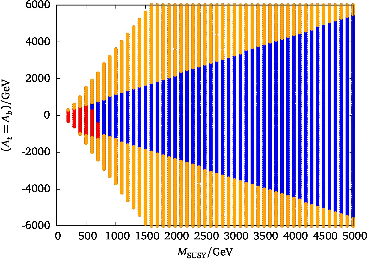
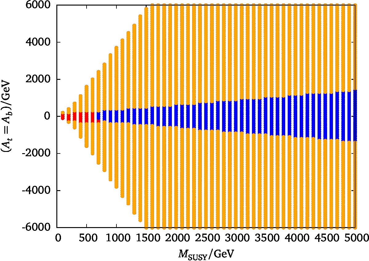
Figure 7: The allowed and excluded regions for varying SUSY masses ${\tilde{m}}_{Q}={\tilde{m}}_{t}=M_{\text{SUSY}}$ and $\tan\beta=40$ (left) as well as $\tan\beta=10$ (right) and $\mu=350\,\mathrm{GeV}$ (both). Blue points do not show any deeper non-standard vacua whereas red and orange do. Orange points have explicitly non-vanishing sbottom vevs. For the purpose of these plots, we have employed SPheno to calculate the spectra.

 

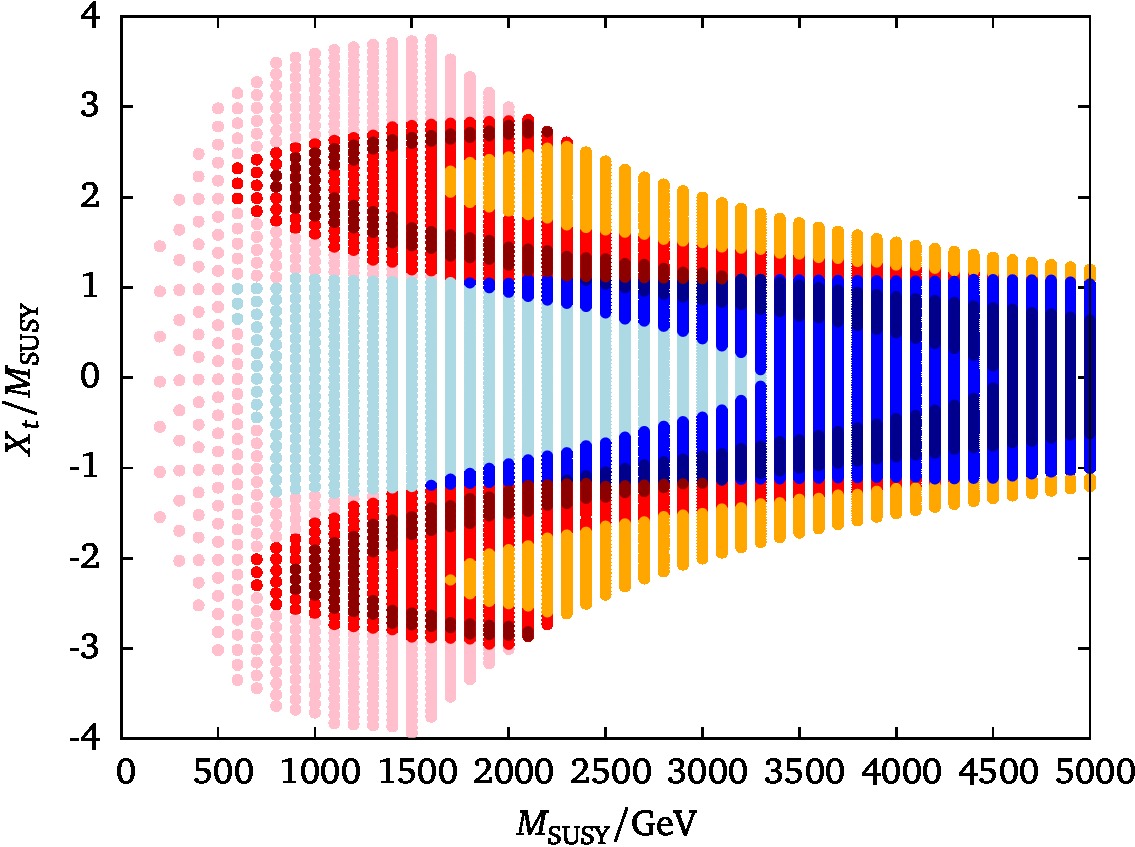
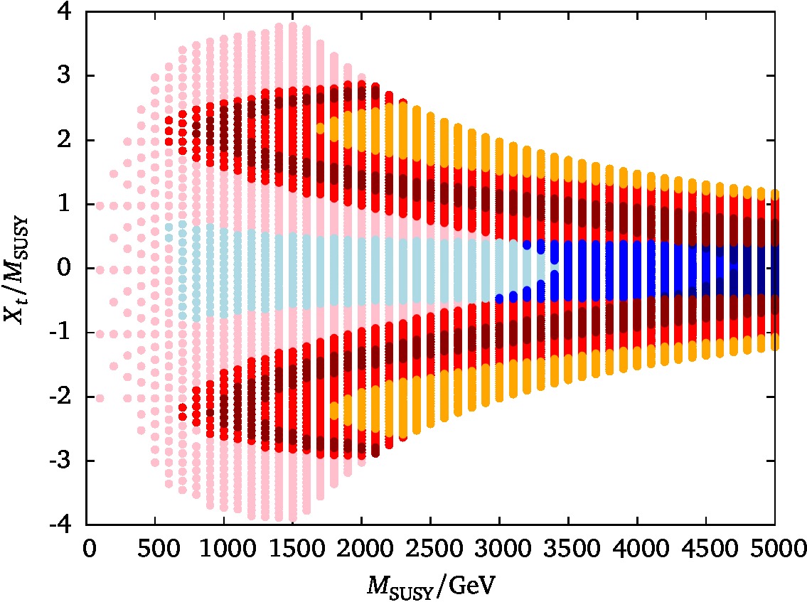
Figure 8: For the inclusion of the Higgs mass prediction in the MSSM, we show the value of $X_{t}/M_{\text{SUSY}}$ varying with the SUSY scale (at $A_{\mathrm{b}}=A_{\mathrm{t}}$ as usually done). On the left side, we kept a low $\mu$-value, $\mu=350\,\mathrm{GeV}$, fixed; whereas on the right side, $\mu$ scales with the SUSY mass, $\mu=M_{\text{SUSY}}$. In both cases we employed $\tan\beta=40$. The color coding shows the compatibility with the Higgs mass measurements: the darker the color the more compatible (the dark blue and red regions indicate $m_{h^{0}}\in[124,126]\,\mathrm{GeV}$ as produced by SPheno corresponding to a $1\,\mathrm{GeV}$ uncertainty; the neighboring region has the $3\,\mathrm{GeV}$ uncertainty). The blueish region is allowed by vacuum stability considerations whereas the reddish region is excluded. For fixed $\mu=350\,\mathrm{GeV}$ that means roughly $|X_{t}|\leq 1.1M_{\text{SUSY}}$; in the case with $\mu=M_{\text{SUSY}}$ the allowed area shrinks with increasing SUSY scale.

 

SUSY hides behind the corner

The question that remains is how much do these bounds depend on the SUSY scale. So far, we have employed $M_{\text{SUSY}}=1\,\mathrm{TeV}$ which needs large $A_{\mathrm{t}}$ close to the border line in order to get $m_{h^{0}}$ right and what points towards near-criticality also in the MSSM. There is of course one way out to still consider the MSSM (with the assumptions applied in this work) as valid and alive. We find that the constraints get weaker with increasing $M_{\text{SUSY}}$, especially the value of the ratio $X_{t}/M_{\text{SUSY}}$ for which a model point would be excluded stays rather constant or even grows for fixed $\mu$ whereas it shrinks with larger $\mu$. This shrinking is not surprising, as $\mu$ enters $X_{t}$ and can enhance its value for various configurations. Similarly, the value of the tree-level $\tan\beta$ enters severely as can be seen from Fig. 7, where we compare the allowed and excluded regions of $A_{\mathrm{t}}=A_{\mathrm{b}}$ with respect to $M_{\text{SUSY}}$ for $\tan\beta=40$ and $10$.. In addition, the proper value for the lightest Higgs mass, $m_{h^{0}}\approx 125\,\mathrm{GeV}$ selects a small band in $X_{t}$-$M_{\text{SUSY}}$. We clearly see from Fig. 8, where the spectrum has been determined with the help of SPheno, that only for SUSY masses that are anyway not yet excluded by experiment in the simplified analyses $M_{\text{SUSY}}\geq 1500\,\mathrm{GeV}$ (for a small $\mu$-term and rather large $\tan\beta$), we can enter the correct range. Increasing $\mu$ shifts the allowed regime to even larger $M_{\text{SUSY}}$. It is therefore with hindsight not surprising at all, that there have been no signals of SUSY found so far in combination to the measured light Higgs mass. Without this additional crucial ingredient one might get depressed seeing the parameter space being closed, especially when the trilinear soft SUSY breaking couplings are taken equally large, $A_{\mathrm{b}}=A_{\mathrm{t}}$, as usually done. One the other hand, this is exactly what is observed by the non-observation of light stops so far. Very light squarks (below say $1\,\mathrm{TeV}$) in connection with large squark mixing are inconsistent with a stable electroweak vacuum. In that sense, SUSY awaits her discovery in the very near future.

4 Conclusions

We have reported on a new view of charge and color breaking minima in the Minimal Supersymmetric Standard Model and consequently derived novel bounds on the parameter space from the self-consistency of the theory. In order to avoid any configurations that lead to an unstable electroweak ground state, large portions of the available parameter space are excluded. We have argued that the exclusions cannot be treated as metastability bounds requiring only a life-time of the false vacuum of about the age of the universe and any CCB exclusion an MSSM parameters is to be seen strict. We have extended the exhaustive work of Ref. [27] mostly by relaxing the constraint on $h_{\mathrm{d}}$ to be strictly smaller than $h_{\mathrm{u}}$ but lacking simple analytic expressions to cover the numerical exclusions. By analyzing both Higgs and third generation squark directions simultaneously (four fields), we cannot fix the signs of the trilinear terms to make them positive. This in addition opens a new window to exclude larger parameter regions as $h_{\mathrm{d}}=-h_{\mathrm{u}}$ is allowed and particularly enhances the effect for certain sign combinations. A generic analytic bound on the four-field level is rather impossible; the remaining freedom, however, allows not to be too restrictive and especially allow for short-lived vacua in formerly metastable parameter regions.

Finally, we have included the determination of the light Higgs mass in the MSSM and find that a low superpartner spectrum (especially light stops) in combination with a $125\,\mathrm{GeV}$ Higgs is excluded by the formation of non-standard vacua around the SUSY scale. A stable electroweak vacuum at the low scale requests (depending on the specific scenario) SUSY masses to be in the multi-TeV regime, $M_{\text{SUSY}}\gtrsim 1.5,\dotsc,6\,\mathrm{TeV}$, for positive $\mu$-values and sizeable $A_{\mathrm{b}}$. Exclusions get weakened for smaller or vanishing $A_{\mathrm{b}}$. Variations on the bounds with rising $M_{\text{SUSY}}$ are given in Fig. 9. Further investigation is needed in very special corners of the parameter space see Fig. 10: negative and small values of $\mu$ keep the window for a $125\,\mathrm{GeV}$ Higgs and squark masses below $1\,\mathrm{TeV}$ open (say $0\geq\mu\geq-1000\,\mathrm{GeV}$, as already indicated in Fig. 6 for $A_{\mathrm{t}}\approx A_{\mathrm{b}}\approx\pm 1500\,\mathrm{GeV}$).

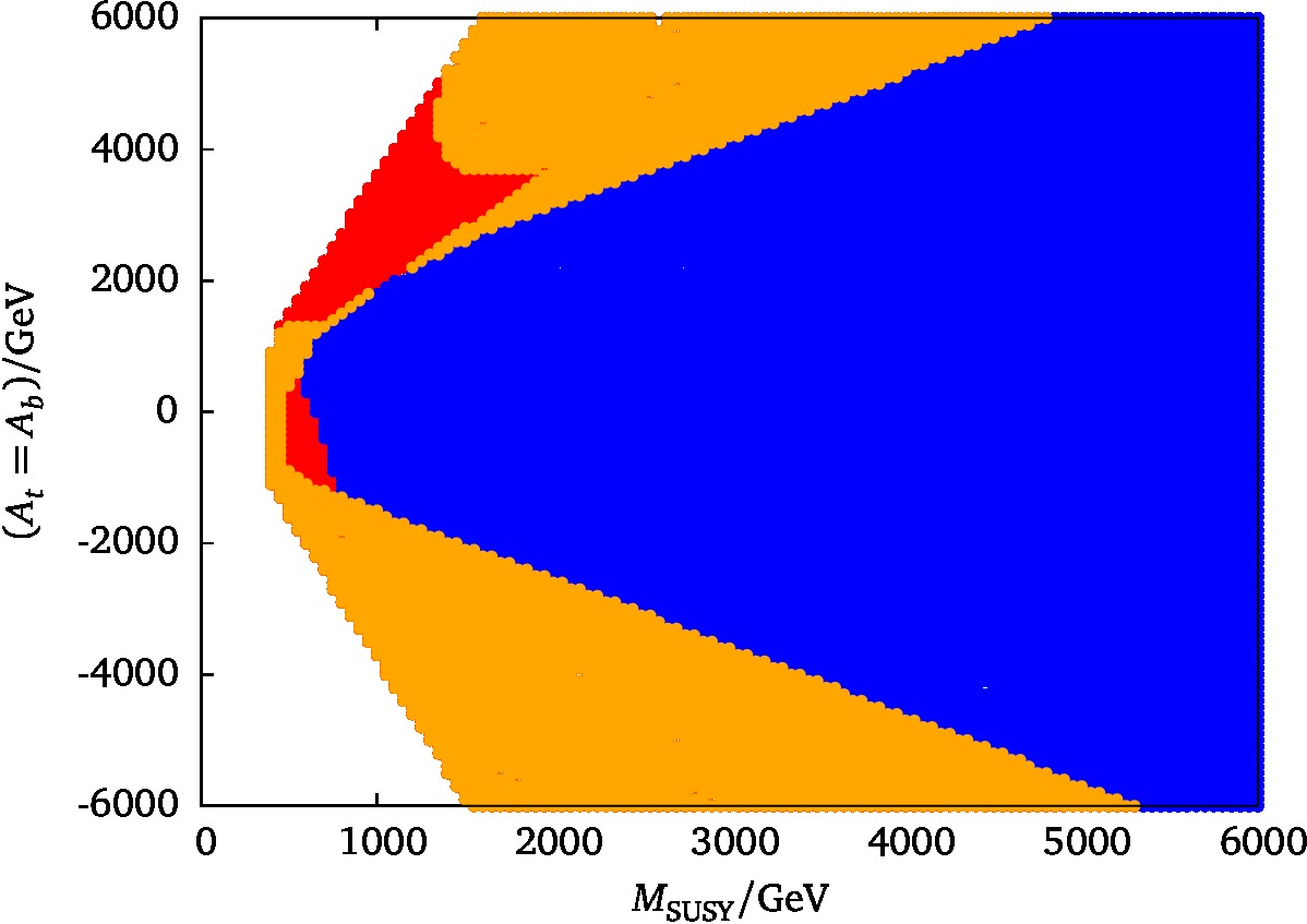
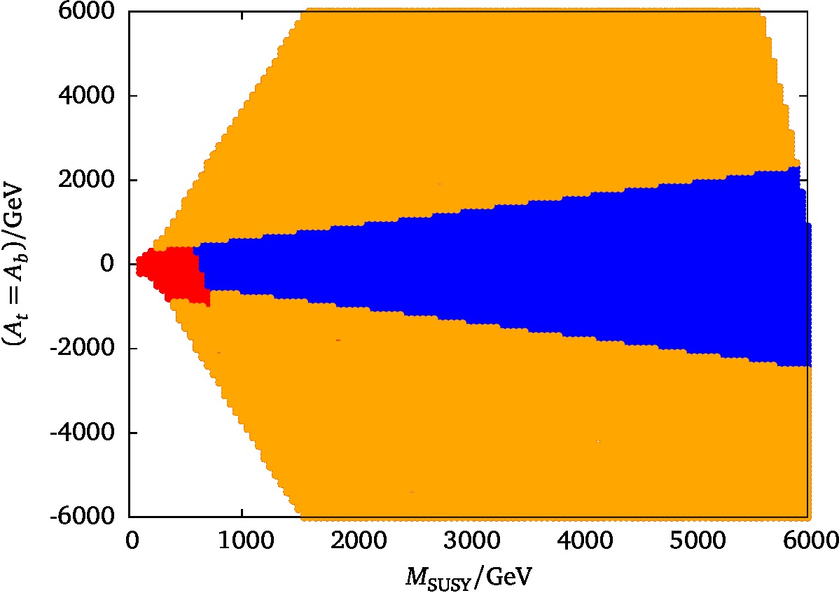
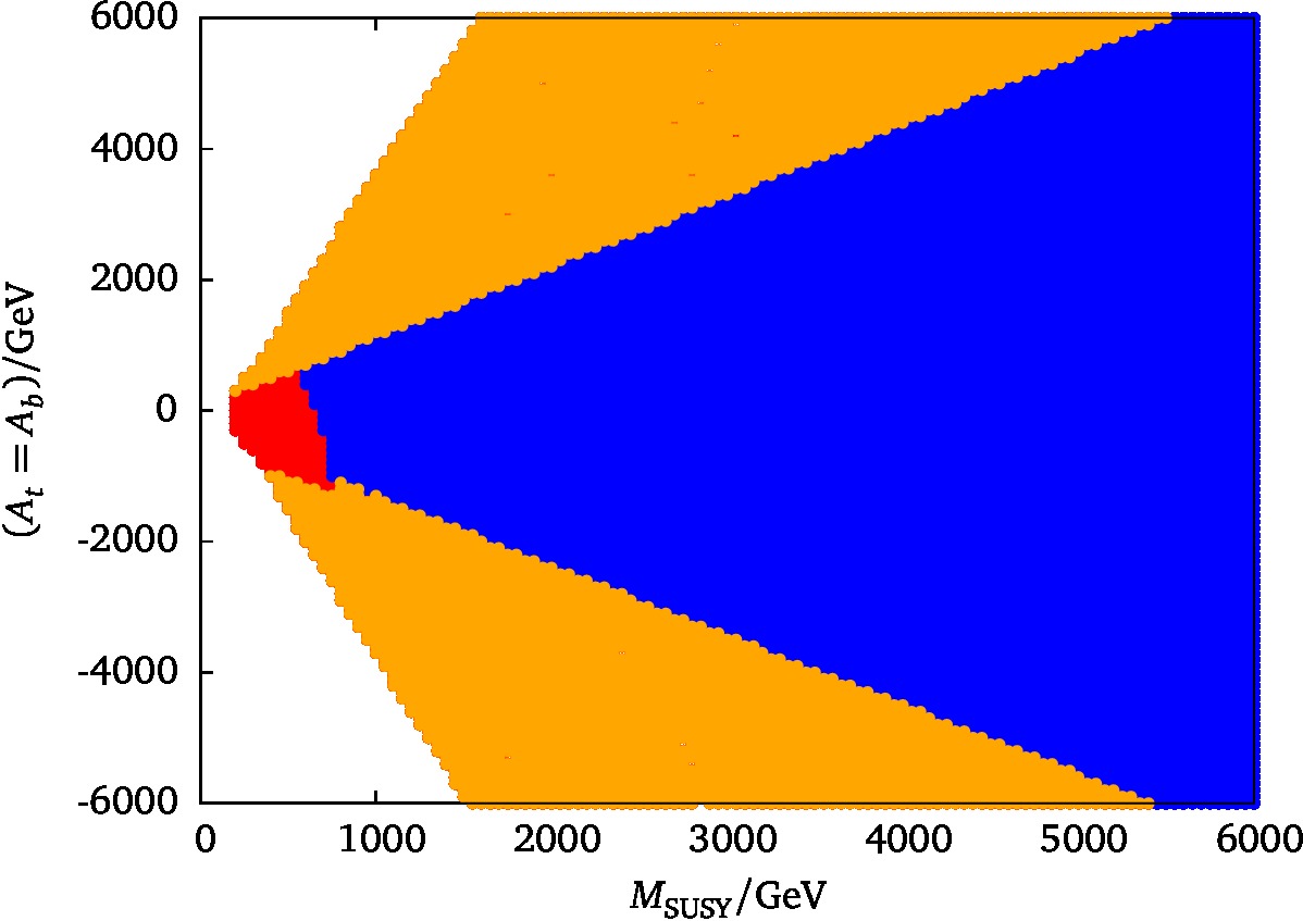
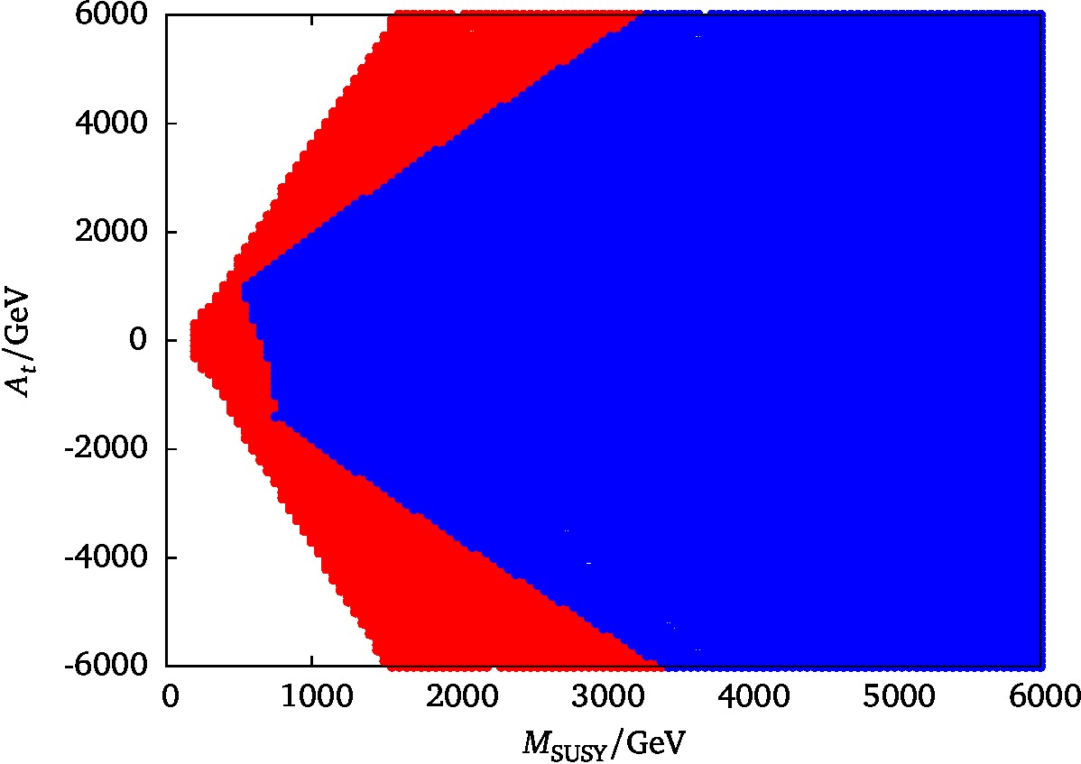
Figure 9: Variations of Fig. 7, all with $\tan\beta=40$ and $m_{A}=800\,\mathrm{GeV}$. All but the lower right have $A_{\mathrm{b}}=A_{\mathrm{t}}$, in the lower right plot we have set $A_{\mathrm{b}}=0\,\mathrm{GeV}$. For the upper left, we keep a negative $\mu$-value $\mu=-500\,\mathrm{GeV}$ fixed, where the upper right has a varying $\mu=M_{\text{SUSY}}$, where the lower left has $\mu=350\,\mathrm{GeV}$ fixed. Color coding as in Fig. 7.

 

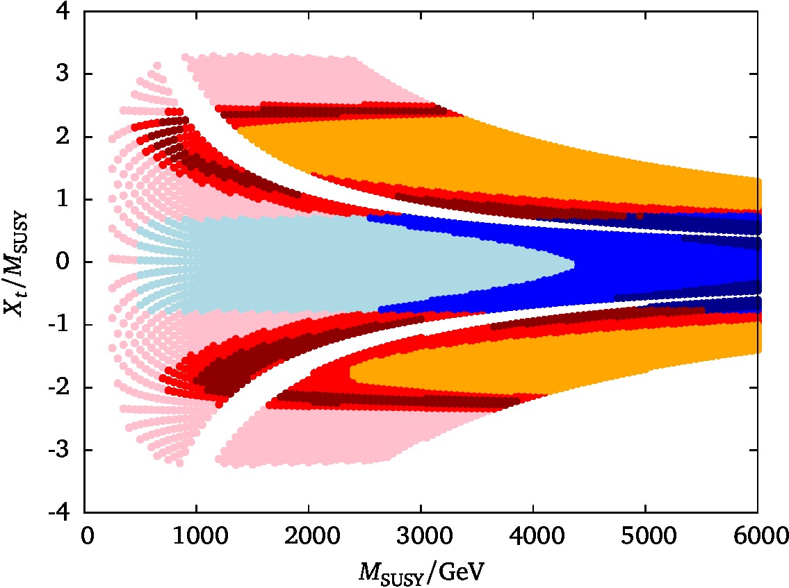
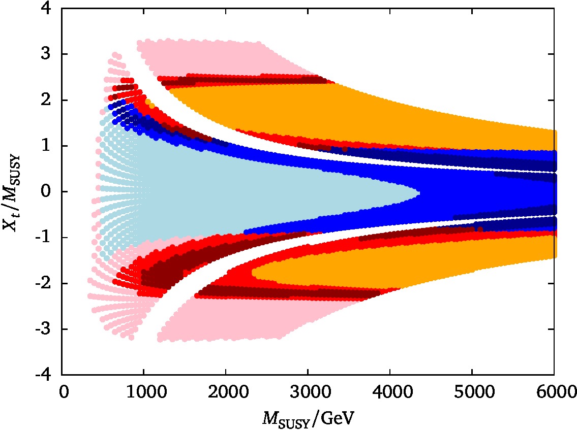
Figure 10: Variations of Fig. 8 with $\tan\beta=40$ and $\mu=350\,\mathrm{GeV}$ (left) as well as $\mu=-500\,\mathrm{GeV}$ (right). The light CP-even Higgs mass has been calculated with the help of FeynHiggs and $m_{\tilde{g}}=1.5M_{\text{SUSY}}$, $m_{A}=800\,\mathrm{GeV}$. The white stripes are left blank because the one-loop effective potential of [42] develops an imaginary part already at the standard vevs and a tachyonic sbottom mass there.

References

- [1] ATLAS Collaboration collaboration, G. Aad et al., Observation of a new particle in the search for the Standard Model Higgs boson with the ATLAS detector at the LHC, Phys.Lett. B716 (2012) 1–29, [1207.7214].
- [2] CMS Collaboration collaboration, S. Chatrchyan et al., Observation of a new boson at a mass of 125 GeV with the CMS experiment at the LHC, Phys.Lett. B716 (2012) 30–61, [1207.7235].
- [3] ATLAS, CMS collaboration, G. Aad et al., Measurements of the Higgs boson production and decay rates and constraints on its couplings from a combined ATLAS and CMS analysis of the LHC collision data at 7 and 8 TeV, 1606.02266.
- [4] S. Weinberg, Implications of Dynamical Symmetry Breaking, Phys.Rev. D13 (1976) 974–996.
- [5] S. Weinberg, Implications of Dynamical Symmetry Breaking: An Addendum, Phys. Rev. D19 (1979) 1277–1280.
- [6] E. Gildener, Gauge Symmetry Hierarchies, Phys. Rev. D14 (1976) 1667.
- [7] L. Susskind, Dynamics of Spontaneous Symmetry Breaking in the Weinberg-Salam Theory, Phys.Rev. D20 (1979) 2619–2625.
- [8] J. Elias-Miro, J. R. Espinosa, G. F. Giudice, G. Isidori, A. Riotto et al., Higgs mass implications on the stability of the electroweak vacuum, Phys.Lett. B709 (2012) 222–228, [1112.3022].
- [9] G. Degrassi, S. Di Vita, J. Elias-Miro, J. R. Espinosa, G. F. Giudice et al., Higgs mass and vacuum stability in the Standard Model at NNLO, JHEP 1208 (2012) 098, [1205.6497].
- [10] M. Zoller, Vacuum stability in the SM and the three-loop -function for the Higgs self-interaction, in What We Would Like LHC to Give Us (A. Zichichi, ed.), pp. 557–566, World Scientific, 2014.
- [11] K. Chetyrkin and M. Zoller, -function for the Higgs self-interaction in the Standard Model at three-loop level, JHEP 1304 (2013) 091, [1303.2890].
- [12] V. Branchina and E. Messina, Stability, Higgs Boson Mass and New Physics, Phys.Rev.Lett. 111 (2013) 241801, [1307.5193].
- [13] V. Branchina, E. Messina and A. Platania, Top mass determination, Higgs inflation, and vacuum stability, JHEP 1409 (2014) 182, [1407.4112].
- [14] B. A. Kniehl, A. F. Pikelner and O. L. Veretin, Two-loop electroweak threshold corrections in the Standard Model, Nucl. Phys. B896 (2015) 19–51, [1503.02138].
- [15] S. Di Vita and C. Germani, Electroweak vacuum stability and inflation via nonminimal derivative couplings to gravity, Phys. Rev. D93 (2016) 045005, [1508.04777].
- [16] L. Di Luzio, G. Isidori and G. Ridolfi, Stability of the electroweak ground state in the Standard Model and its extensions, Phys. Lett. B753 (2016) 150–160, [1509.05028].
- [17] R. N. Mohapatra and G. Senjanovic, Neutrino Mass and Spontaneous Parity Violation, Phys.Rev.Lett. 44 (1980) 912.
- [18] Y. Chikashige, R. N. Mohapatra and R. D. Peccei, Spontaneously Broken Lepton Number and Cosmological Constraints on the Neutrino Mass Spectrum, Phys. Rev. Lett. 45 (1980) 1926.
- [19] J. Schechter and J. Valle, Neutrino Decay and Spontaneous Violation of Lepton Number, Phys.Rev. D25 (1982) 774.
- [20] R. Kuchimanchi and R. N. Mohapatra, No parity violation without R-parity violation, Phys. Rev. D48 (1993) 4352–4360, [hep-ph/9306290].
- [21] J. Frere, D. Jones and S. Raby, Fermion Masses and Induction of the Weak Scale by Supergravity, Nucl.Phys. B222 (1983) 11.
- [22] J. Gunion, H. Haber and M. Sher, Charge / Color Breaking Minima and a-Parameter Bounds in Supersymmetric Models, Nucl.Phys. B306 (1988) 1.
- [23] M. Drees, M. Gluck and K. Grassie, A New Class of False Vacua in Low-energy Supergravity Theories, Phys.Lett. B157 (1985) 164.
- [24] H. Komatsu, New Constraints on Parameters in the Minimal Supersymmetric Model, Phys.Lett. B215 (1988) 323.
- [25] P. Langacker and N. Polonsky, Implications of Yukawa unification for the Higgs sector in supersymmetric grand unified models, Phys. Rev. D50 (1994) 2199–2217, [hep-ph/9403306].
- [26] A. Strumia, Charge and color breaking minima and constraints on the MSSM parameters, Nucl. Phys. B482 (1996) 24–38, [hep-ph/9604417].
- [27] J. Casas, A. Lleyda and C. Munoz, Strong constraints on the parameter space of the MSSM from charge and color breaking minima, Nucl.Phys. B471 (1996) 3–58, [hep-ph/9507294].
- [28] C. Le Mouel, Optimal charge and color breaking conditions in the MSSM, Nucl.Phys. B607 (2001) 38–76, [hep-ph/0101351].
- [29] C. Le Mouel and G. Moultaka, Novel electroweak symmetry breaking conditions from quantum effects in the MSSM, Nucl.Phys. B518 (1998) 3–36, [hep-ph/9711356].
- [30] P. Ferreira, A Full one loop charge and color breaking effective potential, Phys.Lett. B509 (2001) 120–130, [hep-ph/0008115].
- [31] P. Ferreira, Minimization of a one loop charge breaking effective potential, Phys.Lett. B512 (2001) 379–391, [hep-ph/0102141].
- [32] P. Ferreira, One-loop charge and colour breaking associated with the top Yukawa coupling, hep-ph/0406234.
- [33] M. Claudson, L. J. Hall and I. Hinchliffe, Low-Energy Supergravity: False Vacua and Vacuous Predictions, Nucl.Phys. B228 (1983) 501.
- [34] A. Kusenko, P. Langacker and G. Segre, Phase transitions and vacuum tunneling into charge and color breaking minima in the MSSM, Phys.Rev. D54 (1996) 5824–5834, [hep-ph/9602414].
- [35] J. Casas and S. Dimopoulos, Stability bounds on flavor violating trilinear soft terms in the MSSM, Phys.Lett. B387 (1996) 107–112, [hep-ph/9606237].
- [36] J.-h. Park, Metastability bounds on flavour-violating trilinear soft terms in the MSSM, Phys.Rev. D83 (2011) 055015, [1011.4939].
- [37] C. L. Wainwright, CosmoTransitions: Computing Cosmological Phase Transition Temperatures and Bubble Profiles with Multiple Fields, Comput. Phys. Commun. 183 (2012) 2006–2013, [1109.4189].
- [38] J. Camargo-Molina, B. O’Leary, W. Porod and F. Staub, Vevacious: A Tool For Finding The Global Minima Of One-Loop Effective Potentials With Many Scalars, Eur.Phys.J. C73 (2013) 2588, [1307.1477].
- [39] D. Chowdhury, R. M. Godbole, K. A. Mohan and S. K. Vempati, Charge and Color Breaking Constraints in MSSM after the Higgs Discovery at LHC, JHEP 1402 (2014) 110, [1310.1932].
- [40] U. Chattopadhyay and A. Dey, Exploring MSSM for Charge and Color Breaking and Other Constraints in the Context of Higgs@125 GeV, JHEP 11 (2014) 161, [1409.0611].
- [41] N. Blinov and D. E. Morrissey, Vacuum Stability and the MSSM Higgs Mass, JHEP 1403 (2014) 106, [1310.4174].
- [42] M. Bobrowski, G. Chalons, W. G. Hollik and U. Nierste, Vacuum stability of the effective Higgs potential in the Minimal Supersymmetric Standard Model, Phys.Rev. D90 (2014) 035025, [1407.2814].
- [43] W. G. Hollik, Charge and color breaking constraints in the Minimal Supersymmetric Standard Model associated with the bottom Yukawa coupling, Phys. Lett. B752 (2016) 7–12, [1508.07201].
- [44] W. Altmannshofer, M. Carena, N. R. Shah and F. Yu, Indirect Probes of the MSSM after the Higgs Discovery, JHEP 01 (2013) 160, [1211.1976].
- [45] J. E. Camargo-Molina, B. Garbrecht, B. O’Leary, W. Porod and F. Staub, Constraining the Natural MSSM through tunneling to color-breaking vacua at zero and non-zero temperature, Phys. Lett. B737 (2014) 156–161, [1405.7376].
- [46] J. Camargo-Molina, B. O’Leary, W. Porod and F. Staub, Stability of the CMSSM against sfermion VEVs, JHEP 1312 (2013) 103, [1309.7212].
- [47] W. Altmannshofer, C. Frugiuele and R. Harnik, Fermion Hierarchy from Sfermion Anarchy, JHEP 1412 (2014) 180, [1409.2522].
- [48] E. Bagnaschi, F. Brummer, W. Buchmuller, A. Voigt and G. Weiglein, Vacuum stability and supersymmetry at high scales with two Higgs doublets, JHEP 03 (2016) 158, [1512.07761].
- [49] ATLAS, CMS collaboration, G. Aad et al., Combined Measurement of the Higgs Boson Mass in Collisions at and 8 TeV with the ATLAS and CMS Experiments, Phys. Rev. Lett. 114 (2015) 191803, [1503.07589].
- [50] J. R. Ellis, G. Ridolfi and F. Zwirner, Radiative corrections to the masses of supersymmetric Higgs bosons, Phys.Lett. B257 (1991) 83–91.
- [51] R. Barbieri, M. Frigeni and F. Caravaglios, The Supersymmetric Higgs for heavy superpartners, Phys.Lett. B258 (1991) 167–170.
- [52] J. L. Feng, P. Kant, S. Profumo and D. Sanford, Three-Loop Corrections to the Higgs Boson Mass and Implications for Supersymmetry at the LHC, Phys.Rev.Lett. 111 (2013) 131802, [1306.2318].
- [53] M. Carena, S. Heinemeyer, O. Stål, C. E. M. Wagner and G. Weiglein, MSSM Higgs Boson Searches at the LHC: Benchmark Scenarios after the Discovery of a Higgs-like Particle, Eur. Phys. J. C73 (2013) 2552, [1302.7033].
- [54] O. Buchmueller et al., The CMSSM and NUHM1 after LHC Run 1, Eur. Phys. J. C74 (2014) 2922, [1312.5250].
- [55] A. Djouadi and A. Pilaftsis, The 750 GeV Diphoton Resonance in the MSSM, 1605.01040.
- [56] Search for resonances decaying to photon pairs in 3.2 fb-1 of collisions at = 13 TeV with the ATLAS detector, Tech. Rep. ATLAS-CONF-2015-081, CERN, Geneva, Dec, 2015.
- [57] CMS Collaboration collaboration, Search for new physics in high mass diphoton events in proton-proton collisions at TeV, Tech. Rep. CMS-PAS-EXO-15-004, CERN, Geneva, 2015.
- [58] W. G. Hollik, Neutrinos Meet Supersymmetry: Quantum Aspects of Neutrinophysics in Supersymmetric Theories. PhD thesis, Karlsruhe Institute of Technology, 2015. 1505.07764.
- [59] S. R. Coleman and E. J. Weinberg, Radiative Corrections as the Origin of Spontaneous Symmetry Breaking, Phys.Rev. D7 (1973) 1888–1910.
- [60] R. Jackiw, Functional evaluation of the effective potential, Phys.Rev. D9 (1974) 1686.
- [61] D. Buttazzo, G. Degrassi, P. P. Giardino, G. F. Giudice, F. Sala et al., Investigating the near-criticality of the Higgs boson, JHEP 1312 (2013) 089, [1307.3536].
- [62] C. Froggatt and H. B. Nielsen, Standard model criticality prediction: Top mass and Higgs mass , Phys.Lett. B368 (1996) 96–102, [hep-ph/9511371].
- [63] M. J. Duncan and L. G. Jensen, Exact tunneling solutions in scalar field theory, Phys.Lett. B291 (1992) 109–114.
- [64] S. R. Coleman, The Fate of the False Vacuum. 1. Semiclassical Theory, Phys.Rev. D15 (1977) 2929–2936.
- [65] ATLAS collaboration, G. Aad et al., Search for neutral Higgs bosons of the minimal supersymmetric standard model in pp collisions at = 8 TeV with the ATLAS detector, JHEP 11 (2014) 056, [1409.6064].
- [66] CMS collaboration, V. Khachatryan et al., Search for neutral MSSM Higgs bosons decaying to a pair of tau leptons in pp collisions, JHEP 10 (2014) 160, [1408.3316].
- [67] T. Hahn, S. Heinemeyer, W. Hollik, H. Rzehak and G. Weiglein, High-Precision Predictions for the Light CP -Even Higgs Boson Mass of the Minimal Supersymmetric Standard Model, Phys. Rev. Lett. 112 (2014) 141801, [1312.4937].
- [68] M. Frank, T. Hahn, S. Heinemeyer, W. Hollik, H. Rzehak et al., The Higgs Boson Masses and Mixings of the Complex MSSM in the Feynman-Diagrammatic Approach, JHEP 0702 (2007) 047, [hep-ph/0611326].
- [69] G. Degrassi, S. Heinemeyer, W. Hollik, P. Slavich and G. Weiglein, Towards high precision predictions for the MSSM Higgs sector, Eur.Phys.J. C28 (2003) 133–143, [hep-ph/0212020].
- [70] S. Heinemeyer, W. Hollik and G. Weiglein, The Masses of the neutral CP - even Higgs bosons in the MSSM: Accurate analysis at the two loop level, Eur.Phys.J. C9 (1999) 343–366, [hep-ph/9812472].
- [71] S. Heinemeyer, W. Hollik and G. Weiglein, FeynHiggs: A Program for the calculation of the masses of the neutral CP even Higgs bosons in the MSSM, Comput.Phys.Commun. 124 (2000) 76–89, [hep-ph/9812320].
- [72] A. J. Bordner, Parameter bounds in the supersymmetric standard model from charge / color breaking vacua, hep-ph/9506409.
- [73] L. J. Hall, R. Rattazzi and U. Sarid, The Top quark mass in supersymmetric SO(10) unification, Phys.Rev. D50 (1994) 7048–7065, [hep-ph/9306309].
- [74] M. S. Carena, M. Olechowski, S. Pokorski and C. Wagner, Electroweak symmetry breaking and bottom - top Yukawa unification, Nucl.Phys. B426 (1994) 269–300, [hep-ph/9402253].
- [75] D. M. Pierce, J. A. Bagger, K. T. Matchev and R.-j. Zhang, Precision corrections in the minimal supersymmetric standard model, Nucl.Phys. B491 (1997) 3–67, [hep-ph/9606211].
- [76] M. S. Carena, D. Garcia, U. Nierste and C. E. Wagner, Effective Lagrangian for the interaction in the MSSM and charged Higgs phenomenology, Nucl.Phys. B577 (2000) 88–120, [hep-ph/9912516].
- [77] W. Porod, SPheno, a program for calculating supersymmetric spectra, SUSY particle decays and SUSY particle production at colliders, Comput.Phys.Commun. 153 (2003) 275–315, [hep-ph/0301101].
- [78] W. Porod and F. Staub, SPheno 3.1: Extensions including flavour, CP-phases and models beyond the MSSM, Comput. Phys. Commun. 183 (2012) 2458–2469, [1104.1573].
- [79] B. Allanach, SOFTSUSY: a program for calculating supersymmetric spectra, Comput.Phys.Commun. 143 (2002) 305–331, [hep-ph/0104145].
- [80] A. Djouadi, J.-L. Kneur and G. Moultaka, SuSpect: A Fortran code for the supersymmetric and Higgs particle spectrum in the MSSM, Comput.Phys.Commun. 176 (2007) 426–455, [hep-ph/0211331].
- [81] P. Marquard and N. Zerf, SLAM, a Mathematica interface for SUSY spectrum generators, Comput.Phys.Commun. 185 (2014) 1153–1171, [1309.1731].