An Efficient Implementation of the Generalized Labeled Multi-Bernoulli Filter

Abstract

This paper proposes an efficient implementation of the generalized labeled multi-Bernoulli (GLMB) filter by combining the prediction and update into a single step. In contrast to an earlier implementation that involves separate truncations in the prediction and update steps, the proposed implementation requires only one truncation procedure for each iteration. Furthermore, we propose an efficient algorithm for truncating the GLMB filtering density based on Gibbs sampling. The resulting implementation has a linear complexity in the number of measurements and quadratic in the number of hypothesized objects.

I Introduction

Multi-object tracking refers to the problem of jointly estimating the number of objects and their trajectories from sensor data. Driven by aerospace applications in the 1960’s, today multi-object tracking lies at the heart of a diverse range of application areas, see for example the texts [1, 2, 3, 4]. The most popular approaches to multi-object tracking are the joint probabilistic data association filter [1], multiple hypothesis tracking [2], and recently, random finite set (RFS) [3, 4].

The RFS approach has attracted significant attention as a general systematic treatment of multi-object systems and provides the foundation for the development of novel filters such as the Probability Hypothesis Density (PHD) filter [5], Cardinalized PHD (CPHD) filter [6], and multi-Bernoulli filters [3, 7, 8]. While these filters were not designed to estimate the trajectories of objects, they have been successfully deployed in many applications including radar/sonar [9], [10], computer vision [11, 12, 13], cell biology [14], autonomous vehicle [15, 16, 17] automotive safety [18, 19], sensor scheduling [20, 21, 22, 23], and sensor network [24, 25, 26].

The introduction of the generalized labeled multi-Bernoulli (GLMB) RFS in [27, 28] has led to the development of the first tractable and mathematically principled RFS-based multi-object tracker. Recent extensions and applications [29, 30, 31, 32, 33, 34, 35, 36], suggest that the GLMB is a versatile model that offers good trade-offs between tractability and fidelity. The GLMB filter exploits the conjugacy (with respect to the standard measurement model) of the GLMB family to propagate forward in time the (labeled) multi-object filtering density [27]. Each iteration of this filter involves an update operation and a prediction operation, both of which result in weighted sums of multi-object exponentials with intractably large number of terms. The first implementation of the GLMB filter truncates these sums by using the $K$-shortest path and ranked assignment algorithms, respectively, in the prediction and update to determine the most significant components [28].

While the original two-staged implementation is intuitive and highly parallelizable, it is structurally inefficient as two independent truncations of the GLMB densities are required. Specifically, in the update, truncation is performed by solving a ranked assignment problem for each predicted GLMB component. Since truncation of the predicted GLMB sum is performed separately from the update, a significant portion of the predicted components would generate updated components with negligible weights. Thus, computations are wasted in solving a large number of ranked assignment problems with at best cubic complexity in the number of measurements.

In this paper, we present an efficient implementation of GLMB filter with linear complexity in the number of measurements, i.e. at least two orders of magnitude less than the original implementation in [28]. In particular, we derive a joint prediction and update that eliminates inefficiencies in the truncation procedures of the original two-staged implementation (this result has been presented at a conference in [37]). More importantly, we propose an efficient technique for truncating the GLMB filtering density based on Gibbs sampling, which also offers an efficient solution to the data association problem and more generally, the ranked assignment problem. Further, we show that the proposed Gibbs sampler has an exponential convergence rate. Naturally, in the joint prediction and update, deterministic ranked assignment algorithms can also be applied to truncate the GLMB filtering density. While both implementations are highly parallelizable, the Gibbs sampler based solution has a linear complexity in the number of measurements whereas deterministic solutions are cubic at best.

The paper is organized as follows. Background on labeled RFS and the GLMB filter is provided in section II. Section III presents the joint prediction and update formulation and the Gibbs sampler based implementation of the GLMB filter. Numerical results are presented in Section IV and concluding remarks are given in Section V.

II Background

This section summarizes the GLMB filter and its implementation. The reader is referred to the original works [27, 28] for detailed expositions.

Throughout this article, we denote a generalization of the Kroneker delta that takes arbitrary arguments such as sets, vectors, integers etc., by

$$\delta_{Y}[X]\triangleq\left\{\begin{array}[]{l}1,\text{ if }X=Y\\ 0,\text{ otherwise}\end{array}\right..$$

The list of variables $X_{m},X_{m+1},...,X_{n}$ is abbreviated as $X_{m:n}$. For a given set $S$, $1_{S}(\cdot)$ denotes the indicator function of $S$, and $\mathcal{F}(S)$ denotes the class of finite subsets of $S$. For a finite set $X$, its cardinality (or number of elements) is denoted by $|X|$, in addition we use the multi-object exponential notation $f^{X}$ for the product $\mathop{\textstyle\prod}_{x\in X}f(x)$, with $f^{\emptyset}=1$. The inner product $\int f(x)g(x)dx$ is denoted by $\left\langle f,g\right\rangle$.

II-A Labeled RFS

From a Bayesian estimation viewpoint the multi-object state is naturally represented as a finite set, and subsequently modeled as an RFS or a simple-finite point process [5]. In this paper we use Mahler’s Finite Set Statistics (FISST) notion of integration/density (which is consistent with measure theoretic integration/density [38]) to characterize RFSs. Treatments of RFS in the context of multi-object filtering can be found in [3, 4].

Consider a state space $\mathbb{X}$, and a discrete space $\mathbb{L}$, let $\mathcal{L}:\mathbb{X}\mathcal{\times}\mathbb{L}\rightarrow\mathbb{L}$ be the projection defined by $\mathcal{L}((x,\ell))=\ell$. Then $\mathcal{L}(\mathbf{x})$ is called the label of the point $\mathbf{x}\in\mathbb{X}\mathcal{\times}\mathbb{L}$, and a finite subset $\mathbf{X}$ of $\mathbb{X}\mathcal{\times}\mathbb{L}$ is said to have distinct labels if and only if $\mathbf{X}$ and its labels $\mathcal{L}(\mathbf{X})=\{\mathcal{L}(\mathbf{x}):\mathbf{x}\in\mathbf{X}\}$ have the same cardinality. The distinct label indicator is defined by

$$\Delta(\mathbf{X})\triangleq\delta_{|\mathbf{X}|}[|\mathcal{L(}\mathbf{X})|]$$

A labeled RFS is a marked simple point process with state space $\mathbb{X}$ and (discrete) mark space $\mathbb{L}$ such that each realization has distinct labels [27, 28]. The distinct labels provide the means to identify trajectories or tracks of individual objects since a trajectory is a time-sequence of states with the same label.

A GLMB is a labeled RFS with state space $\mathbb{X}$ and (discrete) label space $\mathbb{L}$ distributed according to [27, 28]

$$\mathbf{\pi}(\mathbf{X})=\Delta(\mathbf{X})\sum_{\xi\in\Xi}w^{(\xi)}(\mathcal{L}(\mathbf{X}))\left[p^{(\xi)}\right]^{\mathbf{X}}$$ (1)

where $\Xi$ is a given discrete set, each $p^{(\xi)}(\cdot,\ell)$ is a probability density on $\mathbb{X}$, and each $w^{(\xi)}(L)$ is non-negative with $\sum_{\xi\in\Xi}\sum_{L\in\mathcal{F}\!\left(\mathbb{L}\right)}w^{\left(\xi\right)}\!\left(L\right)=1$. Each term in the mixture (1) consists of: a weight $w^{\left(\xi\right)}\!\left(\mathcal{L}\!\left(\mathbf{X}\right)\right)$ that only depends on the labels of the multi-object state $\mathbf{X}$; and a multi-object exponential $\left[p^{(\xi)}\right]^{\mathbf{X}}$ that depends on the entire multi-object state. A salient feature of the GLMB family is its closure under the multi-object Bayes recursion for the standard multi-object transition kernel and likelihood function [27].

Throughout the paper, single-object states are represented by lowercase letters (e.g. $x$, $\mathbf{x}$) while multi-object states are represented by uppercase letters (e.g. $X$, $\mathbf{X}$), symbols for labeled states and their distributions are bolded (e.g. $\mathbf{x}$, $\mathbf{X}$, $\mathbf{\pi}$) to distinguish them from unlabeled ones, spaces are represented by blackboard bold (e.g. $\mathbb{X}$, $\mathbb{Z}$, $\mathbb{L}$).

II-B Multi-object system model

Using the convention from [27], an object is labeled by an ordered pair $\ell=(k,i)$, where $k$ is the time of birth, and $i\in\mathbb{N}$ is a unique index to distinguish objects born at the same time. Thus, the label space for objects born at time $k$ is $\mathbb{B}_{k}\mathbb{\triangleq}\{k\}\times\mathbb{N}$, and an object born at time $k$ has state $\mathbf{x}\in\mathbb{X}\mathcal{\times}\mathbb{B}_{k}$. Moreover, the label space $\mathbb{L}_{k}$ for objects at time $k$ (including those born prior to $k$) is given by $\mathbb{L}_{k}=\mathbb{L}_{k-1}\cup\mathbb{B}_{k}$ (note that $\mathbb{L}_{k-1}$ and $\mathbb{B}_{k}$ are disjoint). A multi-object state $\mathbf{X}$, at time $k$, is a finite subset of $\mathbb{X}\mathcal{\times}\mathbb{L}_{k}$.

For compactness we omit the subscript $k$ for the current time, the next time is indicated by the subscripts ‘$+$’.

Given the multi-object state $\mathbf{X}$ (at time $k$), each state $(x,\ell)\in\mathbf{X}$ either survives with probability $P_{S}(x,\ell)$ and evolves to a new state $(x_{+},\ell_{+})$ (at time $k+1$) with probability density $f_{+}(x_{+}|x,\ell)\delta_{\ell}[\ell_{+}]$ or dies with probability $1-P_{S}(x,\ell)$. The set $\mathbf{Y}$ of new targets born at time $k+1$ is distributed according to the labeled multi-Bernoulli (LMB)

$$\Delta(\mathbf{Y})\left[1_{\mathbb{B}_{\,+}}\,r_{B,+}\right]^{\mathcal{L(}\mathbf{Y})}\left[1-r_{B,+}\right]^{\mathbb{B}_{+}-\mathcal{L(}\mathbf{Y})}p_{B,+}^{\mathbf{Y}},$$ (2)

where $r_{B,+}(\ell_{+})$ is probability that a new object with label $\ell_{+}$ is born, and $p_{B,+}(\cdot,\ell_{+})$ is the distribution of its kinematic state [27]. The multi-object state $\mathbf{X}_{+}$ (at time $k+1$) is the superposition of surviving objects and new born objects. It is assumed that, conditional on $\mathbf{X}$,  objects move, appear and die independently of each other. The expression for the multi-object transition density can be found in [27, 28].

For a given multi-object state $\mathbf{X}$ with distinct labels, each state $(x,\ell)\in\mathbf{X}$ is either detected with probability $P_{D}(x,\ell)$ and generates an observation $z$ with likelihood $g(z|x,\ell)$ or missed with probability $1-P_{D}(x,\ell)$. The multi-object observation at time $k$, $Z=\{z_{1:|Z|}\}$, is the superposition of the observations from detected objects and Poisson clutter with intensity $\kappa$. Assuming that, conditional on $\mathbf{X}$ (with distinct labels), detections are independent of each other and of clutter, the multi-object likelihood is given by [27, 28]

$$g(Z|\mathbf{X})\propto\sum_{\theta\in\Theta}1_{\Theta(\mathcal{L(}\mathbf{X}))}(\theta)\prod\limits_{(x,\ell)\in\mathbf{X}}\psi_{Z_{{}_{\!}}}^{(\theta(\ell))}(x,\ell)$$ (3)

where: $\Theta$ is the set of positive 1-1 maps $\theta:\mathbb{L}\rightarrow\{0$:$|Z|\}$, i.e. maps such that no two distinct labels are mapped to the same positive value; $\Theta(I)\subseteq\Theta$ denotes the set of positive 1-1 maps with domain $I$; and

$$\psi_{\{z_{1:|Z|}\}}^{(j)}(x,\ell)=\left\{\!\begin{array}[]{ll}\!\frac{P_{D}(x,\ell)g(_{\!}z_{j\!}|_{{}_{\!}}x,\ell)}{\kappa(z_{j})},&\!\!\text{if }j\in\left\{1,...,|Z|\right\}\\ \!1-P_{D}(x,\ell),&\!\!\text{if }j=0\end{array}\right.\!\!.$$ (4)

The map $\theta$ specifies which objects generated which measurements, i.e. object $\ell$ generates measurement $z_{\theta(\ell)}\in Z$, with undetected objects assigned to $0$. The positive 1-1 property means that $\theta$ is 1-1 on $\{\ell:\theta(\ell)>0\}$, the set of labels that are assigned positive values, and ensures that any measurement in $Z$ is assigned to at most one object.

II-C GLMB filter

The GLMB filter propagates the multi-object filtering density forward in time, analytically, under the multi-object transition and measurement models. In implementation, the GLMB filtering density is expressed in an alternative form, known as $\delta$-GLMB

$$\mathbf{\pi}(\mathbf{X})=\Delta(\mathbf{X})\sum_{\xi\in\Xi,I\in\mathcal{F}(\mathbb{L})}\omega^{(I,\xi)}\delta_{I}[\mathcal{L(}\mathbf{X})]\left[p^{(\xi)}\right]^{\mathbf{X}},$$ (5)

where $\omega^{(I,\xi)}=w^{(\xi)}(I)$. Each $\xi\in\Xi$ represents a history of association maps $\xi=(\theta_{1:k})$ while each $I\in\mathcal{F}(\mathbb{L})$ represents a set of object labels. Collectively, the weight $\omega^{(I,\xi)}$ and function $p^{(\xi)}$ is called component $(I,\xi)$ of the $\delta$-GLMB.

Given the $\delta$-GLMB filtering density (5) at time $k$, the $\delta$-GLMB prediction density to time $k+1$ is given by [27]

$$\mathbf{\bar{\pi}}_{{}_{\!}+}(_{{}_{\!}}\mathbf{X})=\Delta_{{\!}}(_{{}_{\!}}\mathbf{X}_{{}_{\!}})\!\sum_{\xi,J_{\!},L_{+}}\bar{\omega}_{+}^{(\xi,J,L_{+\!})}\delta_{{}_{\!}J\cup L_{+\!}}[\mathcal{L}(\mathbf{X})]\!\left[\bar{p}_{+}^{(\xi)}\right]^{\mathbf{X}}$$ (6)

where $\xi\in\Xi$, $J\in\mathcal{F}(\mathbb{L})$, $L_{+}\in\mathcal{F}(\mathbb{B}_{+})$, and

$$\!\!\!\bar{\omega}_{+}^{(\xi,J,L_{+\!})}\!\!\! = \!\!\!1_{\mathcal{F}(\mathbb{B}_{{+}})}(L_{+})\text{ }r_{B\!,+}^{L_{\!+\!}}\left[1-r_{B,+}\right]^{\mathbb{B}_{+}-L_{\!+\!}}$$ (7)

$$\!\times \!\!\!\!\sum_{I\in\mathcal{F}(\mathbb{L})}\!\!1_{\mathcal{F}(I)\!}(_{\!}J)\!\left[{}_{\!}\bar{P}_{S}^{(\xi)\!}\right]^{\!J}\!\left[{}_{\!}1\!-\!\bar{P}_{S\!}^{{}_{\!}(_{\!}\xi)\!}\right]^{\!I-J\!}\omega^{(\!I,\xi)}$$

$$\!\!\!\bar{P}_{{}_{\!}S\!}^{(\xi)}(\ell)\!\!\! = \!\!\!\left\langle p^{(\xi)}(\cdot,\ell),P_{S}(\cdot,\ell)\right\rangle$$ (8)

$$\!\!\!\bar{p}_{+}^{(\xi)}(x_{+},\ell_{+})\!\!\! = \!\!\!1_{\mathbb{L}_{\!}}(\ell_{+})\frac{\!\left\langle P_{S}(\cdot,\ell_{+})f_{{}_{\!}+\!}(x_{+}|\cdot,\ell_{+}),p^{(\xi)}(\cdot,\ell_{+})\right\rangle}{\bar{P}_{S}^{(\xi)}(\ell_{+})}$$ (9)

$$+ \!\!\!1_{\mathbb{B}_{+\!}}(\ell_{+})p_{B,+_{{}_{\!}}}(x_{+},\ell_{+}).$$

Moreover, the $\delta$-GLMB filtering density at time $k+1$ is [27]

$$\mathbf{\pi}_{\!Z_{{}_{\!}+}\!}(\mathbf{X})\propto\Delta_{\!}(_{\!}\mathbf{X}_{\!})\!\!\!\sum\limits_{\xi,J_{\!},L_{\!+\!},\theta_{\!+\!}}\!\!\!\omega_{Z_{{}_{\!}+}}^{(_{\!}\xi,J,L_{\!+\!},\theta_{\!+\!})}\delta_{J\cup L_{\!+\!}}[\mathcal{L}(_{\!}\mathbf{X}_{\!})]\!\left[p_{Z_{{}_{\!}+_{\!}}}^{{}_{\!}(_{\!}\xi,\theta_{\!+\!})}{}_{\!}\right]^{\mathbf{X}}\!\!$$ (10)

where $\theta_{+}\in\Theta_{+}$, and

$$\!\!\!\!\!\!\!\!\omega_{Z_{{}_{\!}+}}^{(\xi,J,L_{+\!},\theta_{+\!})}\!\!\! = \!\!\!1_{{\Theta}_{+\!}(J\cup L_{\!+\!})}(\theta_{+})\!\!\left[\bar{\psi}_{Z_{+}}^{(\xi,\theta_{\!+\!})\!}\right]^{\!J\cup L_{+}}\!\!\bar{\omega}_{+}^{(\xi,J,L_{+})}$$ (11)

$$\!\!\!\!\!\!\!\!\bar{\psi}_{Z_{+}}^{(\xi,\theta_{{}_{\!}+_{\!}})}(\ell_{{}_{\!}+_{\!}})\!\!\! = \!\!\!\left\langle\bar{p}_{+}^{(\xi)}(\cdot,\ell_{+}),\psi_{{}_{\!}Z_{{}_{\!}+}}^{(\theta_{+}(\ell_{+}))}(\cdot,\ell_{+})\right\rangle$$ (12)

$$\!\!\!\!\!\!\!\!p_{Z_{+}}^{(\xi,\theta_{{}_{\!}+_{\!}})_{\!}}(x_{{}_{\!}+},\ell_{{}_{\!}+_{\!}})\!\!\! = \!\!\!\frac{\bar{p}_{+}^{(\xi)}(x_{+},\ell_{+})\psi_{Z_{+}}^{(\theta_{+}(\ell_{+}))}(x_{+},\ell_{+})}{\bar{\psi}_{Z_{+}}^{(\xi,\theta_{+})}(\ell_{+})}$$ (13)

Remark.

To be concise, $\bar{\psi}_{Z_{+}}^{(\xi,\theta_{+})}(\ell_{+})$ should be understood as $\bar{\psi}_{Z_{{}_{\!}+}}^{(\xi,\theta_{+}(\ell_{+}))}(\ell_{{}_{\!}+})$ since (12) does not require knowledge of the entire map $\theta_{+}$, but only its value at $\ell_{+}$. Similarly, $p_{Z_{{}_{\!}+}}^{(\xi,\theta_{+})}(x_{+},\ell_{+})$ should be understood as $p_{Z_{+}}^{(\xi,\theta_{+}(\ell_{+}))}(x_{+},\ell_{+})$.

The first implementation of the GLMB filter recursively computes the predicted and update densities at each time step [28]. Since the number of components in the $\delta$-GLMB prediction and filtering densities grows exponentially with time, these densities are truncated by retaining components with largest weights to minimize the $L_{1}$ truncation error [28].

From the $\delta$-GLMB weight prediction (6)-(7), note that each component $(I,\xi)$ generates a new set of “children” $(I,\xi,J,L_{+})$, $J\subseteq I$, $L_{+}\subseteq\mathbb{B}_{+}$, with weights proportional to $[\bar{P}_{S}^{(\xi)}]^{J}[~{}1~{}\!~{}-~{}\!~{}\bar{P}_{S\!}^{(_{\!}\xi)}~{}]^{I\!-\!J}$ $r_{B\!,+\!}^{L_{+}}\left[1-r_{B\!,+}\right]^{\mathbb{B}_{+}-L_{+}}$. Truncating the contribution of component $(I,\xi)$ to the predicted density without exhaustively computing all the children’s weights is performed by solving two separate $K$-shortest path problems. The first finds a prescribed number of surviving label sets $J\subseteq I$ in non-increasing order of $[\bar{P}_{S}^{(\xi)}]^{J}[1-\bar{P}_{S\!}^{(\xi)}]^{I\!-\!J}$, while the second finds a prescribed number of new label sets $L_{+}\subseteq\mathbb{B}_{+}$, in non-increasing order of $r_{B,+\!}^{L_{+}}\left[1-r_{B\!,+\!}\right]^{\mathbb{B}_{+}-L_{\!+\!}}$. This strategy ensures that components with births, which usually have very low weights, are retained.

From the $\delta$-GLMB weight update (10)-(11), note that each prediction component $(\xi,J,L_{+})$ generates a new set of components $(\xi,J,L_{+},\theta_{+})$, $\theta_{+}\in\Theta_{+}(J\cup L_{+})$, with weights proportional to $[\bar{\psi}_{Z_{+}}^{(\xi,\theta_{+})}]^{J\cup L_{+}}$. Truncating the contribution of component $(\xi,J,L_{+})$ to the updated density without exhaustively computing all the components is performed by solving the ranked assignment problem to find a prescribed number of association maps $\theta_{+}$ in non-increasing order of $[\bar{\psi}_{Z_{{}_{\!}+}}^{(\xi,\theta_{+})}]^{J\cup L_{+}}$.

Separating the truncation of the prediction from the update only exploits a priori knowledge (e.g. survival and birth probabilities), consequently, a significant portion of these predicted components would generate updated components with negligible weights. Hence, computations are wasted in solving a large number of ranked assignment problems, which have, at best, cubic complexity in the number of measurements.

III Efficient implementation of the GLMB filter

To avoid propagating prediction components that would generate weak updated components, this section proposes a new implementation of the GLMB filter with a joint prediction and update. This joint strategy only requires one truncation procedure per iteration, while preserving the filtering performance as well as parallelizability. Further, we detail a $\delta$-GLMB truncation approach based on Gibbs sampling that drastically reduces the complexity.

The $\delta$-GLMB joint prediction and update is presented in subsection III-A, followed by a formulation of the $\delta$-GLMB truncation problem in subsection III-B. The ranked assignment and Gibbs sampling solutions to the truncation problem are given in subsections III-C and III-D, followed by implementations details in subsection III-E.

III-A Joint prediction and update

The following Proposition establishes a direct recursion between the components of two GLMB filtering densities at consecutive times (see the Appendix for proof).

Proposition 1.

Given the $\delta$-GLMB filtering density (5) at time $k$, the $\delta$-GLMB filtering density at time $k+1$ is given by

$$\mathbf{\pi}_{\!Z_{{}_{\!}+}\!}(\mathbf{X})\!\propto\Delta_{\!}(_{\!}\mathbf{X}_{\!})\!\!\!\!\sum\limits_{I\!,\xi,I_{\!+},\theta_{\!+\!}}\!\!\!\!\omega^{(I,\xi)}\omega_{Z_{{}_{\!}+}}^{(_{\!}I_{\!},\xi,I_{\!+\!},\theta_{\!+\!})}\delta_{{}_{\!}I_{+\!}}[\mathcal{L}(_{\!}\mathbf{X}_{\!})]\!\left[p_{Z_{{}_{\!}+_{\!}}}^{(_{\!}\xi,\theta_{\!+\!})}{}_{\!}\right]^{\!\mathbf{X}}\!\!\!$$ (14)

where $I\in\mathcal{F}(\mathbb{L})$, $\xi\in\Xi$, $I_{+}\in\mathcal{F}(\mathbb{L}_{+}),\theta_{+}\in\Theta_{+}$, and

$$\!\!\!\!\!\!\omega_{Z_{{}_{\!}+}}^{(_{\!}I_{\!},\xi,I_{\!+\!},\theta_{\!+\!})}\!\!\! = \!\!\!1_{{\Theta}_{\!+\!}(I_{+})}(\theta_{\!+\!})\!\left[1-\bar{P}_{S}^{(\xi)}\right]^{\!I\!-I_{\!+}}\!\left[\bar{P}_{S\!}^{(\xi)}\right]^{\!I\cap I_{+\!}}$$ (15)

$$\times \!\!\!\left[1-r_{B\!,+}\right]^{\mathbb{B}_{\!+\!}-I_{\!+}\!}r_{B\!,+}^{\mathbb{B}_{\!{+}}\cap I_{+\!}}\!\left[\bar{\psi}_{{}_{\!}Z_{{}_{\!}+}}^{(_{\!}\xi,\theta_{{}_{\!}+\!})}\right]^{I_{+}}$$

$$\!\!\!\!\!\!\bar{P}_{S\!}^{(\xi)}(\ell)\!\!\! = \!\!\!\left\langle p^{(\xi)\!}(\cdot,\ell),P_{S}(\cdot,\ell)\right\rangle$$ (16)

$$\!\!\!\!\!\!\bar{\psi}_{{}_{\!}Z_{{}_{\!}+}}^{(\xi,\theta_{+\!})}(\ell_{{}_{\!}+\!})\!\!\! = \!\!\!\left\langle\bar{p}_{+}^{(\xi)}(\cdot,\ell_{{}_{\!}+}),\psi_{{}_{\!}Z_{{}_{\!}+}\!}^{(\theta_{{}_{\!}+}(\ell_{{}_{\!}+}))}(\cdot,\ell_{{}_{\!}+})\right\rangle$$ (17)

$$\!\!\!\!\!\!\bar{p}_{+}^{(\xi)_{\!}}(x_{{}_{\!}+},\ell_{{}_{\!}+\!})\!\!\! = \!\!\!1_{\mathbb{L}_{\!}}(\ell_{{}_{\!}+\!})\frac{\!\left\langle P_{S}(\cdot,\ell_{{}_{\!}+\!})f_{{}_{\!}+\!}(x_{{}_{\!}+}|\cdot,\ell_{{}_{\!}+\!}),p^{(\xi)}(\cdot,\ell_{{}_{\!}+\!})\right\rangle}{\bar{P}_{S}^{(\xi)}(\ell_{{}_{\!}+})}$$ (18)

$$+ \!\!\!1_{\mathbb{B}_{+}}\!(\ell_{{}_{\!}+_{\!}})p_{B,+_{{}_{\!}}}(x_{{}_{\!}+},\ell_{{}_{\!}+})$$

$$\!\!\!\!\!\!p_{Z_{{}_{\!}+}}^{(\xi_{\!},\theta_{\!+\!})\!}(x_{{}_{\!}+},\ell_{{}_{\!}+\!})\!\!\! = \!\!\!\frac{\bar{p}_{+}^{(\xi)}(x_{{}_{\!}+},\ell_{{}_{\!}+})\psi_{Z_{+}}^{(\theta_{{}_{\!}+}(\ell_{{}_{\!}+}))}(x_{{}_{\!}+},\ell_{{}_{\!}+})}{\bar{\psi}_{Z_{+}}^{(\xi,\theta_{{}_{\!}+})}(\ell_{{}_{\!}+})}.$$ (19)

The summation (14) can be interpreted as an enumeration of all possible combinations of births, deaths and survivals together with associations of new measurements to hypothesized labels. Observe that (14) does indeed take on the $\delta$-GLMB form when rewritten as a sum over $I_{+},\xi,\theta_{+}$ with weights

$$\omega_{Z_{+}}^{(I_{+},\xi,\theta_{+})}\propto\sum\limits_{I}\omega^{(I,\xi)}\omega_{Z_{+}}^{(I,\xi,I_{+},\theta_{+\!})}.$$ (20)

Hence at the next iteration we only propagate forward the components $(I_{+},\xi,\theta_{+})$ with weights $\omega_{Z_{{}_{\!}+}}^{(I_{+},\xi,\theta_{+})}$.

The number of components in the $\delta$-GLMB filtering density grows exponentially with time, and needs to be truncated at every time step, ideally, by retaining those with largest weights since this minimizes the $L_{1}$ approximation error [28]. Note from the $\delta$-GLMB recursion (14)-(15) that each component $(I,\xi)$ generates a set of “children” $(I,\xi,I_{+},\theta_{+})$, $(I_{+},\theta_{+})\in\mathcal{F}(\mathbb{L}_{+})\times\Theta_{+}(I_{+})$ with weights proportional to $\omega_{Z_{{}_{\!}+}}^{(I,\xi,I_{+},\theta_{+})}$. Truncating the contribution of component $(I,\xi)$ to the $\delta$-GLMB filtering density, at time $k+1$, amounts to selecting its “children” $(I,\xi,I_{+},\theta_{+})$ with significant weights.

III-B GLMB truncation formulation

In this and the next two subsections, we consider a fixed component $(\xi,$ $I)$ of the $\delta$-GLMB filtering density at time $k$, and a fixed measurement set $Z_{+}$ at time $k+1$. Specifically, we enumerate $Z_{+}=\{z_{1:M}\}$, $I=\{\ell_{1:R}\}$, and in addition $\mathbb{B}_{{+}\!}=\{\ell_{R+1:P}\}$. The goal is to find a set of pairs $(I_{+},\theta_{+})\in\mathcal{F}(\mathbb{L}_{+})\times\Theta_{+}(I_{+})$ with significant $\omega_{Z_{{}_{\!}+}}^{(I,\xi,I_{+},\theta_{+})}$.

Figure 1: The cost matrix $C$ for the joint prediction and update optimal assignment problem of component $(\xi,$ $I)$. The 3 partitions correspond to survived and detected objects, survived and misdetected objects, and objects that died or not born. The assignment matrix $S$ has the same structure, but with 1’s and 0’s as entries.

For each pair $(I_{+},\theta_{+})\in\mathcal{F}(\mathbb{L}_{+})\times\Theta_{+}(I_{+})$, we define a $P$-tuple $\gamma=(\gamma_{1:P})\in\{-1$:$M\}^{P}$ by

$$\gamma_{i}=\left\{\begin{array}[]{ll}\theta_{+}(\ell_{i}),&\text{if }\ell_{i}\in I_{+}\\ -1,&\text{otherwise}\end{array}\right.$$

Note that $\gamma$ inherits, from $\theta_{+}$, the positive 1-1 property, i.e., there are no distinct $i$, $i^{\prime}\in\{1$:$P\}$ with $\gamma_{i}\!=\!\gamma_{i^{\prime}}>0$. The set of all positive 1-1 elements of $\{-1$:$M\}^{P}$ is denoted by ${\Gamma}$. From $\gamma\in{\Gamma}$, we can recover $I_{+}$ and $\theta_{+}:I_{+}\rightarrow\{0$:$M\}$, respectively, by

$$I_{+}=\{\ell_{i}\in I\cup\mathbb{B}_{\!{+}\!}:\gamma_{i}\geq 0\}\text{ and }\theta_{+}(\ell_{i})=\gamma_{i}.$$ (21)

Thus, $1_{{\Gamma}}(\gamma)=1_{{}_{\!}{\Theta}_{+}(I_{+})}(\theta_{+})$, and there is a 1-1 correspondence between the spaces $\Theta_{+}(I_{+})$ and ${\Gamma}$.

Assuming that for all $i\in\{1$:$P\}$, $\bar{P}_{S}^{(\xi)\!}(\ell_{i})\in(0,1)$ and $\bar{P}_{{}_{\!}D}^{(\xi)\!}(\ell_{i})\triangleq\left\langle\bar{p}_{+}^{(\xi)\!}(\cdot,\ell_{i}),P_{{}_{\!}D}(\cdot,\ell_{i})\right\rangle\in(0,1)$, we define

$$\eta_{i}(j)\!=\!\begin{cases}1-\bar{P}_{S}^{(\xi)\!}(\ell_{i}),&\!1\leq i\leq R,\text{ }j\!<0\!,\\ \bar{P}_{S\!}^{(\xi)\!}(\ell_{i})\bar{\psi}_{Z_{+_{\!}}}^{(\xi,j)\!}(\ell_{i\!}),&\!1\leq i\leq R,\text{ }j\!\geq 0,\\ 1-r_{B\!,+}(\ell_{i}),&\!R\!+\!1\leq i\leq P,\text{ }j\!<0,\\ r_{B\!,+}(\ell_{i})\bar{\psi}_{Z_{+}}^{(\xi,j)}(\ell_{i}),&\!R\!+\!1\leq i\leq P,\text{ }j\!\geq 0.\end{cases}$$ (22)

where $\bar{\psi}_{Z_{+}}^{(\xi,j)}(\ell_{i})\!=\!\left\langle\bar{p}_{+}^{(\xi)}(\cdot,\ell_{i}),\psi_{{}_{\!}Z_{+}}^{(j)}(\cdot,\ell_{i})\right\rangle$, and $j\in\{-1$:$M\}$ is the index of the measurement assigned to label $\ell_{i}$, with $j=0$ indicating that $\ell_{i}$ is misdetected, and $j=-1$ indicating that $\ell_{i}$ no longer exists. It is implicit that $\eta_{i}(j)$ depends on the given $(\xi,$ $I)$ and $Z_{+}$, which have been omitted for compactness. The assumptions on the expected survival and detection probabilities, $\bar{P}_{S}^{(\xi)\!}(\ell_{i})$ and $\bar{P}_{D}^{(\xi)\!}(\ell_{i})$, eliminates trivial and ideal sensing scenarios, as well as ensuring $\eta_{i}(j)>0$.

Note from (21) that since $\theta_{+}(\ell_{i})$ = $\gamma_{i}$, we have $\bar{\psi}_{Z_{+}}^{(\xi,\gamma_{i})}(\ell_{i})$ = $\bar{\psi}_{Z_{+}}^{(\xi,\theta_{+}(\ell_{i}))}(\ell_{i})$ = $\bar{\psi}_{Z_{+}}^{(\xi,\theta_{+})}(\ell_{i})$, (see (12) and the subsequent remark), hence it follows from (22) that

$$\prod\limits_{n=1}^{R}\eta_{n}(\gamma_{n})\!\! = \!\!\left[1-\bar{P}_{S}^{(\xi)}\right]^{I-I_{+}}\left[\bar{P}_{S}^{(\xi)}\bar{\psi}_{Z_{+}}^{(\xi,\theta_{+})}\right]^{I\cap I_{+}}\!,$$

$$\prod\limits_{n=R+1}^{P}\!\eta_{n}(\gamma_{n})\!\! = \!\!\left[1-r_{B\!,+}\right]^{\mathbb{B}_{+}-I_{+}}\left[r_{B\!,+}\bar{\psi}_{Z_{+}}^{(\xi,\theta_{+})}\right]^{\mathbb{B}_{{+}}\cap I_{+}}\!.$$

Moreover, using (15), we have

$$\omega_{Z_{+}}^{(I,\xi,I_{+},\theta_{+})}=1_{{\Gamma}}(\gamma)\prod\limits_{i=1}^{P}\eta_{i}(\gamma_{i}).$$ (23)

Consequently, finding a set of $(I_{+},\theta_{+})\in\mathcal{F}(\mathbb{L}_{+})\times\Theta_{+}(I_{+})$ with significant $\omega_{Z_{{}_{\!}+}}^{(I,\xi,I_{+},\theta_{+})}$ is equivalent to finding a set of positive 1-1 vectors $\gamma$ with significant $\mathop{\textstyle\prod}\nolimits_{i=1\!}^{P}\eta_{i}(\gamma_{i})$.

III-C Ranked Assignment

Similar to the GLMB update implementation in [28], for a given component $(I,\xi)$, the $T$ best positive 1-1 vectors $\gamma$ in non-increasing order of $\prod\nolimits_{i=1}^{P}\eta_{i}(\gamma_{i})$, can be obtained, without exhaustive enumeration, by solving the following ranked assignment problem.

Each $\gamma\in{\Gamma}$ can be represented by a $P\!\times\!(M+2P)$ assignment matrix $S$ consisting of $0$ or $1$ entries with every row summing to $1$, and every column summing to either $1$ or $0$. Note that $S$ can be partitioned into 3 sub-matrices similar to the matrix shown in Fig. 1. For $(i,j)$ $\in$ $\{1$:$P\}\!\times\!\{1$:$M\}$, $S_{i,j}=1$ when $\gamma_{i}$ $=$ $j$ (i.e. $\ell_{i}$ generates the $j$th measurement). For $(i,j)$ $\in$ $\{1$:$P\}\!\times\!\{M+1$:$M+P\}$, $S_{i,j}=1$ when $\gamma_{i}$ $=$ $0$ and $j=M+i$ (i.e. $\ell_{i}$ not detected). For $(i,j)$ $\in$ $\{1$:$P\}\!\times\!\{M\!+\!P\!+\!1$:$M\!+\!2P\}$, $S_{i,j}=1$ when $\gamma_{i}$ $=$ $-1$ and $j=M\!+\!P\!+\!i$ (i.e. $\ell_{i}$ does not exist). More concisely,

$$S_{i,j}=1_{\{1:M\}}(j)\delta_{\gamma_{i\!}}[j]+\delta_{\!M+i}[j]\delta_{\gamma_{i\!}}[0]+\delta_{\!M+P+i}[j]\delta_{\gamma_{i\!}}[-1].$$

The $P\!\times\!(M+2P)$ cost matrix $C$ of this optimal assignment problem (implicitly depends on $(\xi,$ $I)$ and $Z_{+}$), is given by

$$C_{i,j}=\begin{cases}-\ln\eta_{i}(j)&j\in\{1:M\}\\ -\ln\eta_{i}(0)&j=M+i\\ -\ln\eta_{i}(-1)&j=M+P+i\\ \infty&\text{otherwise}\end{cases}$$ (24)

(see also Fig. 1). The cost of an assignment matrix $S$ is

$$\text{tr}(S^{T}C)=\sum_{i=1}^{P}\sum_{j=1}^{M+2P}C_{i,j}S_{i,j},$$

and is related to the weight of the corresponding positive 1-1 vector $\gamma$ by $\exp\!\left(-\text{tr}(S^{T}C)\right)=\mathop{\textstyle\prod}\nolimits_{i=1\!}^{P}\eta_{i}(\gamma_{i})$.

Note that the cost matrix (24) is an extension of the cost matrix of the GLMB update implementation in [28] to integrate birth, death, survival, detection, misdetection and clutter. A GLMB filter implementation using Murty’s algorithm to solve the above ranked assignment problem has been reported in [37]. The same strategy of solving ranked assignment problems with joint prediction and update was proposed for unlabeled multi-object filtering in [39]. Although this approach does not produce tracks like the GLMB filter, it is still useful in applications such as mapping [15, 16] where the individual trajectories of the landmarks are not required.

Solving the ranked assignment problem with cost matrix $C$, for the $T$ best positive 1-1 vectors can be accomplished by Murty’s algorithm [40] with a complexity of $\mathcal{O}\left(T(M+2P)^{4}\right)$. More efficient algorithms [41], [42] can reduce the complexity to $\mathcal{O}\left(T(M+2P)^{3}\right)$. The main contribution of this article is a much cheaper and simpler algorithm for generating positive 1-1 vectors with high weights.

III-D Gibbs Sampling

The main drawback in using existing ranked assignment algorithms are the high computational cost of generating a sequence of positive 1-1 vectors ordered according to their weights, whilst such ordering is not needed in the $\delta$-GLMB approximation. In this subsection, we propose a more efficient alternative by using Markov Chain Monte Carlo (MCMC) to simulate an unordered set of significant positive 1-1 vectors. In particular, we exploit the Gibbs sampler to break down a complex high-dimensional problem into simple, low-dimensional problems to achieve greater efficiency.

The key idea in the stochastic simulation approach is to consider $\gamma$ as a realization of a random variable distributed according to a probability distribution $\pi$ on $\{-1$:$M\}^{P}$. Candidate positive 1-1 vectors are then generated by independently sampling from $\pi$. Asymptotically, the proportion of samples with probabilities above a given threshold is equal to the probability mass of points with probabilities above that threshold. To ensure that mostly high-weight positive 1-1 vectors are sampled, $\pi$ is constructed so that only positive 1-1 vectors have positive probabilities, and those with high weights are more likely to be chosen than those with low weights. An obvious choice of $\pi$ is one that assigns each positive 1-1 vector a probability proportional to its weight, i.e.

$$\pi(\gamma)\propto 1_{{\Gamma}}(\gamma)\prod\limits_{i=1\!}^{P}\eta_{i}(\gamma_{i})$$ (25)

where ${\Gamma}$ is the set of positive 1-1 vectors in $\{-1$:$M\}^{P}$.

Sampling directly from the distribution (25) is very difficult. MCMC is a widely used technique for sampling from a complex distribution by constructing a suitable Markov chain. Indeed, MCMC simulation has been applied to compute posterior distributions of data association variables in multi-object tracking problems [43]. However, depending on the proposal, it could take some time for a new sample to be accepted. Designing a proposal to have high acceptance probability is still an open area of research. Furthermore, the actual distribution of the samples from a Markov chain depends on the starting value, even if asymptotically the samples are distributed according to the stationary distribution. Usually, an MCMC simulation is divided into two parts: the pre-convergence samples, known as burn-ins, are discarded; and the post-convergence samples are used for inference [44]. The key technical problem is that there are no bounds on the burn-in time nor reliable techniques for determining when convergence has occurred, see e.g. [44] and references therein.

The Gibbs sampler is a computationally efficient special case of the Metropolis-Hasting MCMC algorithm, in which proposed samples are always accepted [45, 46]. Further, in GLMB filtering, we are not interested in the distribution of the positive 1-1 vectors. Regardless of their distribution, all distinct positive 1-1 vectors will reduce the $L_{1}$ GLMB approximation error. Thus, unlike MCMC posterior inference, there are no problems with burn-ins.

 

Algorithm 1. Gibbs

• input: $\gamma^{(1)},T,\eta=[\eta_{i}(j)]$

• output: $\gamma^{(1)},...,\gamma^{(T)}$

 

$P:=\mathsf{size}(\eta,1);\quad M:=\mathsf{size}(\eta,2)-2;$

for $t=2:T$

for $n=1:P$

$\gamma_{n}^{(t)}\sim\pi_{n}(\cdot|\gamma_{1:n-1}^{(t)},\gamma_{n+1:P}^{(t-1)})$;

end

$\gamma^{(t)}:=[\gamma_{1}^{(t)},...,\gamma_{P}^{(t)}];$

end

 

Formally, the Gibbs sampler (see Algorithm 1) is a Markov chain $\{\gamma^{(t)}\}_{t=1}^{\infty}$ with transition kernel [45, 46]

$$\pi(\gamma^{\prime}|\gamma)=\mathop{\displaystyle\prod}\limits_{i=1}^{P}\pi_{n}(\gamma_{n}^{\prime}|\gamma_{1:n-1}^{\prime},\gamma_{n+1:P}),$$

where $\pi_{n}(\gamma_{n}^{\prime}|\gamma_{1:n-1}^{\prime},\gamma_{n+1:P})\propto\pi(\gamma_{1:n}^{\prime},\gamma_{n+1:P})$. In other words, given $\gamma=(\gamma_{1:P})$, the components $\gamma_{1}^{\prime},...,\gamma_{P}^{\prime}$ of the state at the next iterate of the chain, are distributed according to the sequence of conditionals

$$\pi_{1}(\gamma_{1}^{\prime}|\gamma_{{}_{\!}2:P}) \propto\pi(\gamma_{1}^{\prime},\gamma_{{}_{\!}2:P})$$

$$\text{ \ }\vdots$$

$$\pi_{n}(\gamma_{n}^{\prime}|\gamma_{1:n-1}^{\prime},\gamma_{n+1:P}) \propto\pi(\gamma_{1:n}^{\prime},\gamma_{n+1:P})$$

$$\text{ \ }\vdots$$

$$\pi_{P}(\gamma_{P}^{\prime}|\gamma_{1:P-1}^{\prime}) \propto\pi(\gamma_{1:P}^{\prime}).$$

Although the Gibbs sampler is computationally efficient with an acceptance probability of 1, it requires the conditionals $\pi_{n}(\cdot|\cdot)$, $n\in\{1$:$P\}$, to be easily computed and sampled from.

In the following we establish closed form expressions for the conditionals that can be computed/sampled at low cost.

Lemma 2.

Let $\bar{n}=\{1$:$P\}-\{n\}$, $\gamma_{\bar{n}\!}=(\gamma_{{}_{\!}1:n_{\!}-_{\!}1\!},\gamma_{{}_{\!}n_{\!}+_{\!}1:P})$, and ${\Gamma}(\bar{n})$ be the set of all positive 1-1 $\gamma_{\bar{n}}$ (i.e. $\gamma_{\bar{n}}$ for which there are no distinct $i,j\in\bar{n}$ with $\gamma_{i}\!=\!\gamma_{j}\!>\!0$). Then, for any $\gamma\in\{-1$:$M\}^{P}$, $1_{{\Gamma}}(\gamma)$ can be factorized as:

$$1_{{\Gamma}}(\gamma)=1_{{\Gamma}(\bar{n})}(\gamma_{\bar{n}\!})\mathop{\displaystyle\prod}\limits_{i\in\bar{n}}(1-1_{\{1:M\}}(\gamma_{n})\delta_{\gamma_{n}}[\gamma_{i}]).$$ (26)

The proof is given in the Appendix.

Proposition 3.

For each $n\in\{1$:$P\}$,

$$\pi_{n}(\gamma_{n}|\gamma_{\bar{n}})\propto\eta_{n}(\gamma_{n})\mathop{\displaystyle\prod}\limits_{i\in\bar{n}}(1-1_{\{1:M\}}(\gamma_{n})\delta_{\gamma_{n}}[\gamma_{i}]).$$ (27)

Proof: We are interested in highlighting the functional dependence of $\pi_{n}(\gamma_{n}|\gamma_{\bar{n}})$ on $\gamma_{n}$, while its dependence on all other variables is aggregated into the normalizing constant:

$$\pi_{n}(\gamma_{n}|\gamma_{\bar{n}}) \triangleq \frac{\pi(\gamma)}{\pi(\gamma_{\bar{n}})}\propto\pi(\gamma)\propto 1_{{\Gamma}}(\gamma)\prod\limits_{j=1}^{P}\eta_{j}(\gamma_{j})$$

$$= \eta_{n}(\gamma_{n})1_{{\Gamma}}(\gamma)\prod\limits_{j\in\bar{n}}\eta_{j}(\gamma_{j}).$$

Factorizing $1_{{\Gamma}}(\gamma)$ using Lemma 2, gives

$$\!\!\!\!\!\!\!\!\!\!\!\!\!\!\!\!\!\!\!\!\pi_{n}(\gamma_{n}|\gamma_{\bar{n}})$$

$$\propto \!\!\eta_{{}_{\!}n_{\!}}(\gamma_{n})_{\!\!}\mathop{\displaystyle\prod}\limits_{i\in\bar{n}}(1\!-\!1_{\{1:M\}\!}(\gamma_{n})\delta_{\!\gamma_{n}}[\gamma_{i}])1_{{\Gamma}\!(\bar{n})\!}(\gamma_{\!\bar{n}})\!\prod\limits_{j\in\bar{n}}\eta_{j}(\gamma_{j})$$

$$\propto \!\!\eta_{{}_{\!}n_{\!}}(\gamma_{n})_{\!\!}\mathop{\displaystyle\prod}\limits_{i\in\bar{n}}(1\!-\!1_{\{1:M\}\!}(\gamma_{n})\delta_{\!\gamma_{n}}[\gamma_{i}]).\text{ \ \ \ \ \ \ \ \ \ \ \ \ \ \ \ \ \ \ \ }\square$$

For a non-positive $j$, $1_{\{1:M\}\!}(j)=0$, and Proposition 3 implies $\pi_{n}(j|\gamma_{\bar{n}})$ $\propto$ $\eta_{n}(j)$. On the other hand, given any $j$ $\in$ $\{1:M\}$, Proposition 3 implies that $\pi_{n}(j|\gamma_{\bar{n}})$ $\propto$ $\eta_{n}(j)$, unless $j\in\{\gamma_{1:n-1},\gamma_{n+1:P}\}$, i.e. there is an $i\in\bar{n}$ with $\gamma_{i}=j$, in which case $\pi_{n}(j|\gamma_{\bar{n}})=0$. Consequently, for $j$ $\in$ $\{1:M\}$

$$\pi_{n}(j|\gamma_{\bar{n}})\propto\eta_{n}(j)(1-1_{\{\gamma_{1:n-1},\gamma_{n+1:P}\}}(j)).$$

Hence, sampling from the conditionals is simple and inexpensive as illustrated in Algorithm 1a, which has an $\mathcal{O}(PM)$ complexity since sampling from a categorical distribution is linear in the number of categories [47]. Consequently, the complexity of the Gibbs sampler (Algorithm 1) is $\mathcal{O}(TP^{2}M)$.

Proposition 3 also implies that for a given a positive 1-1 $\gamma_{\bar{n}}$, only $\gamma_{n}\in\{-1$:$M\}$ that does not violate the positive 1-1 property can be generated by the conditional $\pi_{n}(\cdot|\gamma_{\bar{n}})$, with probability proportional to $\eta_{n}(\gamma_{n})$. Thus, starting with a positive 1-1 vector, all iterates of the Gibbs sampler are also positive 1-1. If the chain is run long enough, the samples are effectively distributed from (25) as formalized in Proposition 4 (see Appendix for proof).

Proposition 4.

Starting from any initial state in ${\Gamma}$, the Gibbs sampler defined by the family of conditionals (27) converges to the target distribution (25) at an exponential rate. More concisely, let $\pi^{j}$ denote the $j$th power of the transition matrix, then

$$\max_{\gamma,\gamma^{\prime}\in{\Gamma}}(|\pi^{j}(\gamma^{\prime}|\gamma)-\pi(\gamma^{\prime})|)\leq(1-2\beta)^{\left\lfloor\frac{j}{2}\right\rfloor},$$

where $\beta\triangleq\min_{\gamma,\gamma^{\prime}\in{\Gamma}}\pi^{2}(\gamma^{\prime}|\gamma)>0$ is the least likely 2-step transition probability.

 

Algorithm 1a. $\gamma_{n}^{\prime}\sim\pi_{n}(\cdot|\gamma_{1:n-1}^{\prime},\gamma_{n+1:P})$

 

$c:=[-1:M];\quad\eta_{n}:=[\eta_{n}(-1),...,\eta_{n}(M)];$

for $j=1:M$

$\eta_{n}(j):=\eta_{n}(j)(1-1_{\{\gamma_{1:n-1}^{\prime},\gamma_{n+1:P}\}}(j));$

end

$\gamma_{n}^{\prime}\sim\mathsf{Categorical}(c,\eta_{n});$

 

The proposed Gibbs sampler has a short burn-in period due to its exponential convergence rate. More importantly, since we are not using the samples to approximate (25) as in an MCMC inference problem, it is not necessary to discard burn-in and wait for samples from the stationary distribution. For the purpose of approximating the $\delta$-GLMB filtering density, each distinct sample constitutes one term in the approximant, and reduces the $L_{1}$ approximation error by an amount proportional to its weight. Hence, regardless of their distribution, all distinct samples can be used, the larger the weights, the smaller the $L_{1}$ error between the approximant and the true $\delta$-GLMB.

Remark.

The proposed Gibbs sampling solution can be directly applied to the standard data association problem in joint probabilistic data association and multiple hypothesis tracking. Further, it can be adapted to solve a ranked assignment problem with $P$ workers and $M$ jobs as follows. Each assignment is represented by a positive 1-1 vector $\gamma$ in $\{0$:$M\}^{P}$, with $\gamma_{n}=j$ indicating that worker $n$ is assigned job $j$, which incurs a cost $F_{n,j}$. Note that $\gamma_{n}=0$ indicates that worker $n$ is assigned no job, which incurs a cost of $F_{n,0}$ (usually assumed to be 0). The cost of an assignment $\gamma$ is given by $\mathop{\textstyle\sum}\nolimits_{n=1\!}^{P}F_{n,\gamma_{n}}$. Hence, Algorithm 1 can be used to generate a sequence of assignments with significant costs by setting $c:=[0:M]$, and $\eta_{n}=[\eta_{n}(0),...,\eta_{n}(M)]$, where $\eta_{n}(j)=\exp(-F_{n,j})$, in the first line of Algorithm 1a. A sufficient condition for exponential convergence of the Gibbs sampler (i.e. Proposition 4 to hold) is a finite cost of assigning no job to any worker (usually this cost is $0$, i.e. $\eta_{i}(0)=1$). The final step is to remove duplicates and rank the Gibbs samples (according to their costs), which requires additional computations with $\mathcal{O}(T\log T)$ complexity.

III-E Joint Prediction and Update Implementation

A $\delta$-GLMB of the form (5) is completely characterized by parameters $(\omega^{(I,\xi)},p^{(\xi)})$, $(I,\xi)\in\mathcal{F}\!(\mathbb{L})\!\times\!\Xi$, which can be enumerated as $\{(I^{(h)},\xi^{(h)},\omega^{(h)},p^{(h)})\}_{h=1}^{H}$, where

$$\omega^{(h)}\triangleq\omega^{(I^{(h)},\xi^{(h)})},\;p^{(h)}\triangleq p^{(\xi^{(h)})}.$$

Since the $\delta$-GLMB (5) can now be rewritten as

$$\mathbf{\pi}(\mathbf{X})=\Delta(\mathbf{X})\sum\limits_{h=1}^{H}\omega^{(h)}\delta_{I^{(h)}}[\mathcal{L(}\mathbf{X})]\left[p^{(h)}\right]^{\mathbf{X}},$$

there is no need to store $\xi^{(h)}$, and implementing the GLMB filter amounts to propagating forward the parameter set

$$\{(I^{(h)},\omega^{(h)},p^{(h)})\}_{h=1}^{H}.$$

Estimating the multi-object state from the $\delta$-GLMB parameters is the same as in [28].

The procedure for computing the parameter set

$$\{(I_{+}^{(h_{+})},\omega_{+}^{(h_{+})},p_{+}^{(h_{+})})\}_{h_{+}=1}^{H_{+}}$$

at the next time is summarized in Algorithm 2. Note that to be consistent with the indexing by $h$ instead of $(I,\xi)$, we abbreviate

$$\!\!\!\!\!\!\!\bar{P}_{S}^{(h)}(\ell_{{}_{\!}i})\!\! \triangleq \!\!\bar{P}_{{}_{\!}S\!}^{(\xi^{(h)})}(\ell_{{}_{\!}i}),$$

$$\!\!\!\!\!\!\!\bar{p}_{+}^{(h)_{\!}}(x,\ell_{{}_{\!}i})\!\! \triangleq \!\!\bar{p}_{+}^{(\xi^{(h)})_{\!}}(x,\ell_{{}_{\!}i\!}),$$

$$\!\!\!\!\!\!\!\bar{\psi}_{Z_{+}}^{(h,j)}(\ell_{{}_{\!}i})\!\! \triangleq \!\!\bar{\psi}_{Z_{+}}^{(\xi^{(h)},j)}(\ell_{{}_{\!}i})$$

$$\!\!\!\!\!\!\!\eta_{i}^{(h)}(j)\!\! \triangleq \!\!\begin{cases}1-\bar{P}_{S}^{(h)\!}(\ell_{i}),&\!\ell_{i\!}\in I^{(h)},\text{ }j\!<0\!,\\ \bar{P}_{S}^{(h)}(\ell_{i})\bar{\psi}_{Z_{+}}^{(h,j)\!}(\ell_{i\!}),&\!\ell_{i\!}\in I^{(h)},\text{ }j\!\geq 0,\\ 1-r_{B\!,+}(\ell_{i}),&\!\ell_{i\!}\in\mathbb{B}_{+},\text{ }j\!<0,\\ r_{B\!,+}(\ell_{i})\bar{\psi}_{Z_{+}}^{(h,j)\!}(\ell_{i}),&\!\ell_{i\!}\in\mathbb{B}_{+},\text{ }j\!\geq 0.\end{cases}$$ (28)

At time $k+1$, the three main tasks are:

1. Generate $\{(I^{(h_{+})},\xi^{(h_{+})},I_{+}^{(h_{+})},\theta_{+}^{(h_{+})})\}_{h_{+}=1}^{H_{+}}$, the set of “children” with significant weights;

2. Compute $\{(I^{(h_{+})},I_{+}^{(h_{+})},\omega_{+}^{(h_{+})},p_{+}^{(h_{+})})\}_{h_{+}=1}^{H_{+}}$, the intermediate parameter set, as in Proposition 1;

3. Compute $\{(I_{+}^{(h_{+})},\omega_{+}^{(h_{+})},p_{+}^{(h_{+})})\}_{h_{+}=1}^{H_{+}}$, the parameter set at time $k+1$, using (20).

For task 1, using the rationale from subsection III-D, the set of “children” can be generated by sampling from the distribution $\pi$ given by

$$\pi(I,\xi,I_{+},\theta_{+})\propto\omega^{(I,\xi)}\omega_{Z_{{}_{\!}+}}^{(I,\xi,I_{+},\theta_{+})}.$$

This can be achieved by sampling $(I^{(h_{+})},\xi^{(h_{+})})$ from $\pi(I,\xi)\propto\omega^{(I,\xi)}$, and then conditional on $(I^{(h_{+})},\xi^{(h_{+})})$, sample $(I_{+}^{(h_{+})},\theta_{+}^{(h_{+})})$ from $\pi(I_{+},\theta_{+}|I^{(h_{+})},\xi^{(h_{+})})$. Equivalently, in Algorithm 2 we draw $H_{+}^{\max}$ samples $(I^{(h)},\xi^{(h)})$ from $\pi(I,\xi)\propto\omega^{(I,\xi)}$, and then for each distinct sample $(I^{(h)},\xi^{(h)})$ with $T_{+}^{(h)}$ copies, use the Gibbs sampler (Algorithm 2a) to generate $T_{+}^{(h)}$ samples $(I_{+}^{(h,t)},\theta_{+}^{(h,t)})$ from $\pi(I_{+},\theta_{+}|I^{(h)},\xi^{(h)})$. Note that each $(I_{+}^{(h,t)},\theta_{+}^{(h,t)})$ is represented by the positive 1-1 vector $\gamma^{(h,t)}$ (see (21) for the equivalence of this representation).

 

Algorithm 2. Joint Prediction and Update

• input: $\{(I^{(h)},\omega^{(h)},p^{(h)})\}_{h=1}^{H}$, $Z_{+}$, $H_{+}^{\max}$,

• input: $\{(r_{\!B\!,+}^{(\ell)},p_{B\!,+}^{(\ell)})\}_{\ell\in\mathbb{B}_{\!+}}$, $P_{S}$, $f_{\!+\!}(\cdot|\cdot)$, $\kappa_{+}$, $P_{D\!,+}$, $g_{+\!}(\cdot|\cdot)$,

• output: $\{(I_{+}^{(h_{+})},\omega_{+}^{(h_{+})},p_{+}^{(h_{+})})\}_{h_{+}=1}^{H_{+}}$

 

sample counts $[T_{+}^{(h)}]_{h=1}^{H}$  from a multinomial distribution with

parameters $H_{+}^{\max}$ trials and weights ${[}\omega^{(h)}]_{h=1}^{H}$

for $h=1:H$

initialize $\gamma^{(h,1)}$

compute $\eta^{(h)}=[\eta_{i}^{(h)}(j)]_{(i,j)=(1,-1)}^{(|I^{(h)}\!\cup\!\mathbb{B}_{+}|,|Z_{+}|)}$  using (28)

$\{\gamma^{(h,t)}\}_{{}_{t=1}}^{\tilde{T}_{+}^{(h)}}:=\mathsf{Unique(Gibbs}(\gamma^{(h,1)},T_{+}^{(h)},\eta^{(h)}));$

for $t=1:\tilde{T}_{+}^{(h)}$

compute $I_{+}^{(h,t)}$ from $I^{(h)}$ and $\gamma^{(h,t)}$ using (29)

compute $\omega_{+}^{(h,t)}$ from $\omega^{(h)}$ and $\gamma^{(h,t)}$ using (30)

compute $p_{+}^{(h,t)}$ from $p^{(h)}$ and $\gamma^{(h,t)}$ using (31)

end

end

$(\{(I_{+}^{(h_{+})}\!,p_{+}^{(h_{+})})\}_{h_{+}=1}^{H_{+}},\sim,[U_{h,t}])$

$:=\mathsf{Unique}(\{(I_{+}^{(h,t)}\!,p_{+}^{(h,t)})\}_{(h,t)=(1,1)}^{(H,\tilde{T}_{+}^{(h)})});$

for $h_{+}=1:H_{+}$

$\omega_{+}^{(h_{+})}:=\sum\limits_{h,t:U_{h,t}=h_{+}}\omega_{+}^{(h,t)};$

end

normalize weights $\{\omega_{+}^{(h_{+})}\}_{h_{+}=1}^{H_{+}}$

 

 

Algorithm 2a. Gibbs

• input: $\gamma^{(1)},T,\eta=[\eta_{i}(j)]$

• output: $\gamma^{(1)},...,\gamma^{(T)}$

 

$P:=\mathsf{size}(\eta,1);\ M:=\mathsf{size}(\eta,2)-2;\ c:=[-1$:$M];\ \tilde{\eta}:=\eta;$

for $t=2:T$

$\gamma^{(t)}:=[$ $];$

for $n=1:P$

for $j=1:M$

$\tilde{\eta}_{n}(j):=\eta_{n}(j)(1-1_{\{\gamma_{1:n-1}^{(t)},\gamma_{n+1:P}^{(t-1)}\}}(j));$

end

$\gamma_{n}^{(t)}\sim\mathsf{Categorical}(c,\tilde{\eta}_{n});$ $\gamma^{(t)}:=[\gamma^{(t)},\gamma_{n}^{(t)}];$

end

end

 

In task 2, for each $h$, after discarding repeated positive 1-1 vector samples via the “Unique” MATLAB function, the intermediate parameters $(I^{(h)},I_{+}^{(h,t)},\omega_{+}^{(h,t)},p_{+}^{(h,t)})$, $t=1$:$\tilde{T}_{+}^{(h)}$ are computed from the positive 1-1 vector $\gamma^{(h,t)}$ by

$$\!\!\!\!I_{+}^{(h,t)}\!\!\!\! = \!\!\!\!\{\ell_{i}\in I^{(h)}\cup\mathbb{B}_{\!{+}\!}:\gamma_{i}^{(h,t)}\geq 0\},$$ (29)

$$\!\!\!\!\omega_{+}^{(h,t)}\!\!\!\! \propto \!\!\!\!\omega^{(h)}\mathop{\textstyle\prod}\limits_{i=1}^{|I^{(h)}\cup\mathbb{B}_{+}|}\eta_{i}^{(h)}(\gamma_{i}^{(h,t)}),$$ (30)

$$\!\!\!\!p_{+}^{(h,t)\!}(\cdot,\ell_{i})\!\!\!\! = \!\!\!\!\bar{p}_{+}^{(h)}(\cdot,\ell_{i})\psi_{Z_{+}}^{(\gamma_{i}^{(h,t)})}(\cdot,\ell_{i})/\bar{\psi}_{Z_{+}}^{(h,\gamma_{i}^{(h,t)})}(\ell_{i}).$$ (31)

Equations (29)-(31) follow directly from (21), (15)-(19) and (23). Computing $p_{+}^{(h,t)}(\cdot,\ell_{i})$ (and $\eta_{i}^{(h,t)}(j)$, $\bar{\psi}_{Z_{+}}^{(h,j)}(\ell_{i})$, $\bar{P}_{{}_{\!}S\!}^{(h)\!}$) can be done via sequential Monte Carlo or Gaussian mixture, depending on the representation of the densities $p^{(h)}$ (see subsections IV.B and V.B of [28] for details).

Finally, in task 3 the intermediate parameters are marginalized via (20) and the weights normalized, to give the new component set $\{(I_{+}^{(h_{+})},\omega_{+}^{(h_{+})},p_{+}^{(h_{+})})\}_{h_{+}=1}^{H_{+}}$. Note that the output $U_{h,t}$ of the “Unique” MATLAB function gives the index of the GLMB component at time $k+1$ that $(I^{(h)},I_{+}^{(h,t)},p_{+}^{(h,t)})$ contributes to.

Since we are only interested in samples that provide a good representation of the $\delta$-GLMB filtering density, increased efficiency (for the same $H_{+}^{\max}$) can be achieved by using annealing or tempering techniques to modify the stationary distribution so as to induce the Gibbs sampler to seek more diverse samples [51], [52]. One example is to initially decrease the temperature to seek out the nearest mode, and subsequently increase the temperature for diversity.

In scenarios with small birth weights, $\delta$-GLMB components that involve births also have small weights, and are likely to be discarded when $H_{+}^{\max}$ (which depends on the available computing resource) is not large enough, leading to poor track initiation. Increasing the temperature does not guarantee the selection of components with births. Tempering with the birth model (e.g. by feeding the Gibbs sampler with a larger birth rate) directly induces the chain to generate more components with births. Note that the actual weights of the $\delta$-GLMB density components are computed using the correct birth model parameters. Similarly, tempering with the survival probability induces the Gibbs sampler to generate more components with object deaths and improves track termination. Tempering with parameters such as detection probabilities and clutter rate induces the Gibbs sampler to generate components that reduce the occurrence of dropped tracks. Note that if the number of significant components exceeds $H_{+}^{\max}$ the filtering performance will degrade in subsequent iterations.

The Gibbs sampler can be initialized with the highest weighted 1-1 vector (requires solving an optimal assignment problem [53], [54]). Alternatively, a trivial initialization is the all-zeros 1-1 vector (requires no computations). Proposition 4 ensures convergence of the chain to the stationary distribution at an exponential rate regardless of the initialization.

Remark.

It is possible to replace the Gibbs sampler by a deterministic ranked assignment algorithm with cost matrix (24) to generate the $T_{+}^{(h)}$ strongest positive 1-1 vectors, where $T_{+}^{(h)}$ is chosen to be proportional to the weight $\omega^{(h)}$ [37]. Note that such allocation scheme does not necessarily produce the $H_{+}$ best components at time $k+1$. It is possible to discard some children from weaker parents, which still have higher weights than some of those from stronger parents. Other schemes for choosing $T_{+}^{(h)}$ are possible. A ranked assignment problem can also be formulated to find the $H_{+}$ best components. However, the complexity grows and parallelizability is lost. Similar to the Gibbs sampler based solution, tempering with the multi-object model parameters can be used to increase efficiency.

Let $P\triangleq\max_{h}|I^{(h)}\!\cup\!\mathbb{B}|$ and $M\triangleq|Z_{+}|$. The standard and fastest ranked assignment algorithms have respective complexities $\mathcal{O}((2P+M)^{4})$ and $\mathcal{O}((2P+M)^{3})$ i.e. at best, cubic in both the number of hypothesized labels and measurements. On the other hand, the complexity of the Gibbs sampling based solution is $\mathcal{O}(P^{2}M)$, i.e. quadratic in the number of hypothesized labels and linear in the number of measurements.

IV Numerical Studies

This section presents two numerical experiments to verify the proposed GLMB filter implementation without consideration for parallelization. The first demonstrates its efficiency via a linear Gaussian scenario. The second demonstrates its versatility on a very challenging non-linear scenario with non-uniform detection profile and dense clutter.

IV-A Linear Gaussian

The linear Gaussian scenario in the experiment of [28] is used to compare typical speedup in CPU time between the original implementation in [28] and the proposed implementation (Algorithm 2). In summary this scenario involves an unknown and time varying number objects (up to 10 in total) with births, deaths and crossings. Individual object kinematics are described by a 4D state vector of position and velocity that follows a constant velocity model with sampling period of $1s$, and process noise standard deviation $\sigma_{\nu}=5m/s^{2}$. The survival probability $P_{S}=0.99$, and the birth model is an LMB with parameters $\{r_{B,k}(\ell_{i}),p_{B,k}(\ell_{i})\}_{i=1}^{3}$, where $\ell_{i}=(k,i)$, $r_{B,k}(\ell_{i})=0.04$, and $p_{B}(x,\ell_{i})=\mathcal{N}(x;m_{B}^{(i)},P_{B})$ with

$$\begin{array}[]{ll}m_{B}^{(1)}=[0,0,100,0]^{T},&\!\!m_{B}^{(2)}=[-100,0,-100,0]^{T},\\ m_{B}^{(3)}=[100,0,-100,0]^{T},&\!\!P_{B}^{\text{ \ \ \ }}=\mathrm{diag}([10,10,10,10]^{T})^{2}.\end{array}$$

Observations are 2D position vectors on the region $[-1000,1000]m\times[-1000,1000]m$ with noise standard deviation $\sigma_{\varepsilon}=10m$. The detection probability $P_{D}=0.88$ and clutter is modeled as a Poisson RFS with a uniform intensity of $\lambda_{c}=1.65\times 10^{-5}~{}m^{-2}$ on the observation region (i.e. an average of 66 false alarms per scan).

In the original implementation, predicted components are obtained by combining independently generated surviving and births components, together with a CPHD look ahead step for better efficiency (see [28] for full details). To increase diversity of the GLMB components, the proposed implementation with Gibbs sampling uses tempered birth, survival and detection parameters, specifically each $r_{B}(_{\!}\ell_{i\!})$ is increased by a factor of 10, while $P_{S}$ and $P_{D}$ are reduced by 5%. For completeness, the implementation via joint prediction and update with Murty’s algorithm is also considered using the same tempered parameters. All implementations use Gaussian mixture representations of the track densities. We compare the speedup (ratio of CPU times) between the original implementation and the proposed Gibbs sampler based joint prediction and update implementation as well as between the original implementation and the Murty based joint prediction and update implementation. Three cases are considered for various values of $H^{\max}$ (the cap on the number of components) under which the implementations exhibit approximately the same tracking performance (it is virtually impossible for the different implementations to have exactly the same tracking performance). The results reported below are obtained over 100 Monte Carlo trials.

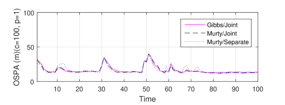
Figure 2: Similar OSPA errors for the three different implementations.

Speedup	Case 1	Case 2	Case 3
Murty/Joint	24X	2.5X	185X
Gibbs/Joint	187X	27X	1443X

Figure 3: Range of CPU time speedup factors compared to the original implementation obtained for various cases.

IV-A1 Case 1

This baseline comparison uses the values of $H^{\max}$ where each implementation starts to exhibit reasonable tracking performance, and have approximately the same average optimal sub-pattern assignment (OSPA) error [55]. The original implementation requires $H^{\max}=10^{4}$ while the joint prediction and update implementation with the proposed Gibbs sampler and Murty’s algorithm both require $H^{\max}=10^{3}$. Fig. 2 confirms that all implementations exhibit approximately similar OSPA curves, except for several pronounced peaks between times $k=55$ and $k=75$ for the original implementation, due to the latter being slower confirm new births. Fig. 3 shows speedups of about two and one orders of magnitude, respectively, for the proposed Gibbs based and Murty based joint prediction and update implementations.

IV-A2 Case 2

All implementations are allocated the same $H^{\max}=10^{4}$. Fig. 3 shows a speedup of over one order of magnitude for the proposed joint prediction and update implementation with Gibbs sampling while there is a small improvement in the Murty based joint prediction and update implementation. Both joint prediction and update implementations now only show a slightly better average OSPA error than the original implementation, confirming that $H^{\max}=10^{3}$ is a good trade-off between computational load and performance.

IV-A3 Case 3

In an attempt to reduce the peaks in the OSPA curve observed in case 1, we raise $H^{\max}$ for the original implementation to $10^{5}$ (the experiment takes too long to run for larger values of $H^{\max}$ to be useful). However, these peaks only reduce slightly and are still worse than both joint prediction and update implementations for $H^{\max}=10^{3}$. Furthermore, the original implementation now only shows a slightly better average OSPA error than the others. In this extreme case Fig. 3 shows speedups of roughly three and two orders of magnitude, respectively, for the Gibbs based and Murty based joint prediction and update implementations.

It should be noted that in general the actual speedup observed depends strongly on the scenario and testing platform, and hence the reported speedup figures should be taken only as broad indication of the range that could be expected. For an indication of the actual speed and accuracy, on real data, against some recent algorithms, we refer the reader to [56].

IV-B Non-linear

This example considers a very challenging scenario in which previous implementations breakdown, specifically the non-linear scenario in the experiment of [27], with reduced detection profile and increased clutter rate. Again there is an unknown and time varying number of objects (up to 10 in total) with births, deaths, and crossings. Individual object kinematics are described by a 5D state vector $x_{k}=[~{}p_{x,k},\dot{p}_{x,k},p_{y,k},\dot{p}_{y,k}~{},\omega_{k}]^{T}$ of planar position, velocity, and turn rate, which follows a coordinated turn model with a sampling period of $1s$ and transition density $f_{k|k-1}(x_{k}|x_{k-1})=\mathcal{N}(x_{k};F(\omega_{k})x_{k},Q)$, where

$$F(\omega)=\left[\begin{array}[]{ccccc}1&\!\!\frac{\sin\omega}{\omega}&0&\!\!-\frac{1-\cos\omega}{\omega}&0\\ 0&\!\!\cos\omega&0&\!\!-\sin\omega&0\\ 0&\!\!\frac{1-\cos\omega}{\omega}&1&\!\!\frac{\sin\omega}{\omega}&0\\ 0&\!\!\sin\omega&0&\!\!\cos\omega&0\\ 0&0&0&0&1\end{array}\right]\!\!,G=\begin{bmatrix}\frac{1}{2}&0\\ 1&0\\ 0&\frac{1}{2}\\ 0&1\end{bmatrix}\!\!,$$

$Q=\mathrm{diag}([\sigma_{w}^{2}GG^{T},\sigma_{u}^{2}])$, $\sigma_{w}=15m/s^{2}$, and $\sigma_{u}=(\pi/180)rad/s$ are the process noise standard deviations. The survival probability $P_{S}=0.99$, and the birth model is an LMB with parameters $\{r_{B,k}(\ell_{i}),p_{B,k}(\ell_{i})\}_{i=1}^{4}$, where $\ell_{i}=(k,i)$, $r_{B,k}(\ell_{1})=r_{B,k}(\ell_{2})=0.02$, $r_{B,k}(\ell_{3})=r_{B,k}(\ell_{4})=0.03$, and $p_{B,k}(x,\ell_{i})=\mathcal{N}(x;m_{B}^{(i)},P_{B})$ with

$$\!\!\!\!\!\!\!\!\!\!\!\!\!\!\begin{array}[]{ll}m_{B}^{(1)}=[-1500,0,250,0,0]^{T},&\!\!m_{B}^{(2)}=[-250,0,1000,0,0]^{T}\\ m_{B}^{(3)}=[250,0,750,0,0]^{T},&\!\!m_{B}^{(4)}=[1000,0,1500,0,0]^{T},\end{array}$$

$$\!\!\!\!\!\!\!\!\!\!\!\!\!\!\begin{array}[]{ll}P_{B}^{\text{ \ \ \ }}=\mathrm{diag}([50,50,50,50,6(\pi/180)]^{T})^{2}.&\end{array}$$

Observations are noisy 2D bearings and range detections $z=[~{}\theta,r~{}]^{T}$ on the half disc of radius $2000m$ with noise standard deviations $\sigma_{r}=5m$ and $\sigma_{\theta}=(\pi/180)rad$ respectively. The detection profile is a (unnormalized) Gaussian with a peak of $0.95$ at the origin and $0.88$ at the edge of surveillance region. Clutter follows a Poisson RFS with a uniform intensity of $\lambda_{c}=1.6\times 10^{-2}$ $(radm)^{-1}$ on the observation region (i.e. an average of 100 false alarms per scan).

The proposed GLMB filter implementation uses particle approximations of the track densities to accommodate nonlinearity and state dependent probability of detection. Again, the birth, survival and detection parameters are tempered, specifically each $r_{B}(\ell_{i\!})$ is increased by a factor of 20, while $P_{S}(x,\ell)$ and $P_{D}(x,\ell)$ are reduced by 5%. Due to the high uncertainty in the scenario, a large $H^{\max}$ is needed since there is a large number of GLMB components with similar weights. Further, the differences between the weights of significant and insignificant components are not as pronounced as the original scenario in [27]. Consequently, the Monte Carlo integration error should be significantly smaller than these differences for the computation of (28) and the weights to be useful. Thus regardless of whether Gibbs sampling or Murty’s algorithm is used, a very large number of particles per object is needed. The tracking result with $H^{\max}=10^{5}$ and 100000 particles per object for a single sample run shown in Fig. 4 illustrates that the proposed GLMB filter implementation successfully track all objects, and is confirmed by the OSPA curve in Fig. 5. Previous implementations break down due to the large number of required components and particles.

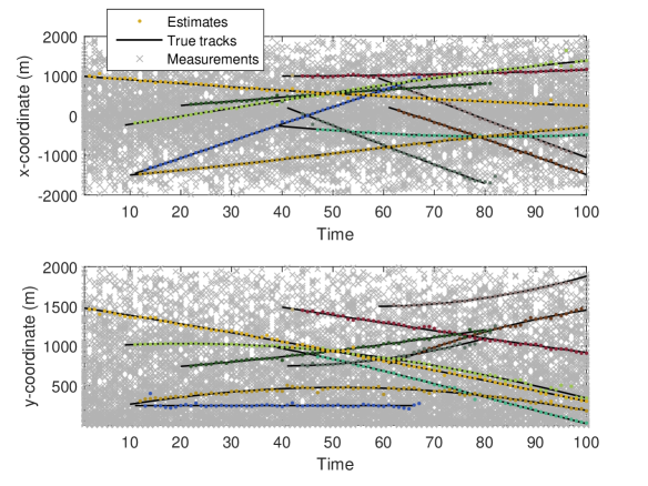
Figure 4: Track estimates, measurements and ground truths for a sample run.

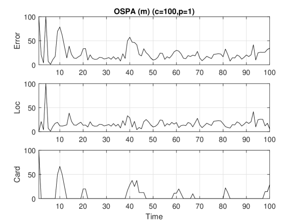
Figure 5: OSPA error for a sample run.

V Conclusions

This paper proposed an efficient implementation of the GLMB filter by integrating the prediction and update into one step along with an efficient algorithm for truncating the GLMB filtering density based on Gibbs sampling. The resulting algorithm is an on-line multi-object tracker with linear complexity in the number of measurements and quadratic in the number of hypothesized tracks, which can accommodate non-linear dynamics and measurements, non-uniform survival probabilities, sensor field of view and clutter intensity. This implementation is also applicable to approximations such as the labeled multi-Bernoulli (LMB) filter since this filter requires a special case of the $\delta$-GLMB prediction and a full $\delta$-GLMB update to be performed [29]. The proposed Gibbs sampler can be adapted to solve the ranked assignment problem and hence the data association problem in other tracking approaches. It is also possible to parallelize the Gibbs sampler [57]. A venue for further research is the generalization of the proposed technique to more complex problems such as multiple extended object tracking [31], or tracking with merged measurements [35].

VI Appendix: Mathematical Proofs

Proof of Proposition 1: Using the change of variable $I_{+\!}=J\cup L_{+}$, we have $J=\mathbb{L}\cap I_{+}$, $L_{+}=\mathbb{B}_{\!{+}\!}\cap I_{+}$, and hence (11) becomes

$$\omega_{Z_{{}_{\!}+}}^{\!(J,L_{\!+\!,}\xi,\theta_{\!+\!})}\!\!\! = \!\!\!\omega_{Z_{{}_{\!}+}}^{(\mathbb{L}\cap I_{+},\mathbb{B}_{{+}}\cap I_{+}\xi,\theta_{\!+})}$$

$$= \!\!\!1_{{}_{\!}{\Theta}_{\!+\!}(I_{+})}(\theta_{\!+\!})\!\left[{}_{\!}\bar{\psi}_{{}_{\!}Z_{{}_{\!}+}}^{(\xi,\theta_{{}_{\!}+})\!}\right]^{\!I_{+}}\!\bar{\omega}_{+}^{(\mathbb{L}\cap I_{+},\mathbb{B}_{{+}}\cap I_{+},_{\!}\xi)}$$

$$= \!\!\!1_{{}_{\!}{\Theta}_{\!+\!}(I_{+})}(\theta_{\!+\!})\!\left[{}_{\!}\bar{\psi}_{{}_{\!}Z_{{}_{\!}+}}^{(\xi,\theta_{{}_{\!}+})\!}\right]^{\!I_{+}}$$

$$\times \!\!\!1_{\!\mathcal{F}_{{}_{\!}}(_{{}_{\!}}\mathbb{B}_{\!{+}\!})\!}(\mathbb{B}_{\!{+}\!}\cap\!I_{+})\text{ }r_{B,+}^{\mathbb{B}_{\!{+}\!}\cap\!I_{+}}\left[1-r_{B,+}\right]^{\mathbb{B}_{+}-(\mathbb{B}_{{+}}\cap\!I_{+})}$$

$$\times \!\!\!\sum_{I}\!1_{\!\mathcal{F}\!(I)\!}(\mathbb{L}\!\cap\!I_{+\!})\!\!\left[{}_{\!}\bar{P}_{S\!}^{{}_{\!}(_{\!}\xi)\!}\right]^{\!\mathbb{L}\cap\!I_{+}}\!\!\left[{}_{\!}1\!-\!\bar{P}_{S\!}^{{}_{\!}(_{\!}\xi)\!}\right]^{\!I\!-(\mathbb{L}\cap\!I_{\!+\!})\!}\!\omega^{(\!I,\xi)}$$

$$= \!\!\!1_{{}_{\!}{\Theta}_{\!+\!}(I_{+\!})}(_{\!}\theta_{\!+\!})\!\left[{}_{\!}\bar{\psi}_{{}_{\!}Z_{{}_{\!}+}}^{(\xi,\theta_{{}_{\!}+\!})\!}\right]^{\!I_{+}}\!r_{B,+}^{\mathbb{B}_{{+}}\cap I_{+}}\left[1-r_{B,+\!}\right]^{\mathbb{B}_{+}-I_{+\!}}$$

$$\times \!\!\!\sum_{I}\left[{}_{\!}\bar{P}_{S\!}^{(\xi)\!}\right]^{\!I\cap I_{+\!}}\!\left[{}_{\!}1\!-\!\bar{P}_{S\!}^{(\xi)\!}\right]^{\!I\!-I_{+}\!}\omega^{(I,\xi)}$$

where the last equality follows from $1_{\mathcal{F}(_{{}_{\!}}\mathbb{B}_{\!{+}\!})}(\mathbb{B}_{\!{+}}\cap I_{+})=1$, $\mathbb{B}_{+}-(\mathbb{B}_{\!{+}}\cap I_{+})=\mathbb{B}_{\!+\!}-I_{\!+}$, and $\mathbb{L}\cap I_{+}=I\cap I_{+}$, $I\!-\!(\mathbb{L}\cap I_{+})=I\!-\!I_{\!+}$ for any $I_{+}$ such that $1_{\mathcal{F}(I)}(\mathbb{L}\cap I_{+})=1$. Further, substituting the above equation into (10) and noting that $J$, $L_{\!+\!}$ are disjoint, the sum over the pair $J$, $L_{\!+}$ reduces to the sum over $I_{\!+}$. Hence, exchanging the order of the sums gives the desired result. $\square$

Proof of Lemma 2: Note that $\gamma_{i}\!=\!\gamma_{j}\!>\!0$ iff $\delta_{\gamma_{i\!}}[\gamma_{j}]1_{\{1:M\}}(\gamma_{i})=1$. Hence, $\gamma$ is positive 1-1 iff for any distinct $i$, $j$, $\delta_{\gamma_{i\!}}[\gamma_{j}]1_{\{1:M\}}(\gamma_{i})=0$. Also, $\gamma$ is not positive 1-1 iff there exists distinct $i$, $j$ such that $\delta_{\gamma_{i}\!}[\gamma_{j}]1_{\{1:M\}}(\gamma_{i})=1$. Similarly, $\gamma_{\bar{n}\!}$ is positive 1-1 iff for any distinct $i$, $j\in\bar{n}$, $\delta_{\gamma_{i\!}}[\gamma_{j}]1_{\{1:M\}}(\gamma_{i})=0$.

We will show that (a) if $\gamma$ is positive 1-1 then the right hand side (RHS) of (26) equates to 1, and  (b) if $\gamma$ is not positive 1-1, then the RHS of (26) equates to 0.

To establish (a), assume that $\gamma$ is positive 1-1, then $\gamma_{\bar{n}\!}$ is also positive 1-1, i.e., $1_{{\Gamma}(\bar{n})}(\gamma_{\bar{n}\!})=1$, and for any $i\neq n$, $\delta_{\gamma_{n\!}}[\gamma_{i}]1_{\{1:M\}}(\gamma_{n})=0$. Hence the RHS of (26) equates to 1.

To establish (b), assume that $\gamma$ is not positive 1-1. If $\gamma_{\bar{n}\!}$ is also not positive 1-1, i.e., $1_{{\Gamma}(\bar{n})}(\gamma_{\bar{n}\!})=0$, then the RHS of (26) trivially equates to 0. It remains to show that even if $\gamma_{\bar{n}\!}$ is positive 1-1, the RHS of (26) still equates to 0. Since $\gamma$ is not positive 1-1, there exist distinct $i$, $j$ such that $\delta_{\gamma_{i\!}}[\gamma_{j}]1_{\{1:M\}}(\gamma_{i})=1$. Further, either $i$ or $j$ has to equal $n$, because the positive 1-1 property of $\gamma_{\bar{n}\!}$ implies that if such (distinct) $i$, $j$, are in $\bar{n}$, then $\delta_{\gamma_{i\!}}[\gamma_{j}]1_{\{1:M\}}(\gamma_{i})=0$ and we have a contradiction. Hence, there exists $i\neq n$ such that $\delta_{\gamma_{n\!}}[\gamma_{i}]1_{\{1:M\}}(\gamma_{n})=1$, and thus the RHS of (26) equates to 0. $\square$

Proof of Proposition 4: Convergence of finite state Markov chains can be characterized in terms of irreducibility and regularity. Following [48], a Markov chain is irreducible if it is possible to move from any state to any other state in finite time, further, an irreducible finite state Markov chain is regular if some finite power of its transition matrix has all positive entries.

Consider the $n$th conditional $\pi_{n}(\gamma_{n}^{\prime}|\gamma_{1:n-1}^{\prime},\gamma_{n+1:P})$, with $\gamma^{\prime}$ positive 1-1. Then for each $j\in\{1$:$n\!-\!1\}$, $1_{\{1:M\}}(\gamma_{j}^{\prime})\delta_{\gamma_{n}^{\prime}}[\gamma_{j}^{\prime}]=0$, hence it follows from (27) that

$$\!\!\!\!\!\!\!\!\!\!\!\!\!\!\!\!\!\!\!\!\!\!\!\!\!\!\!\!\!\!\!\!\!\!\pi_{n}(\gamma_{n}^{\prime}|\gamma_{1:n-1}^{\prime},\gamma_{n+1:P})$$ (34)

$$= \frac{\eta_{n}(\gamma_{n}^{\prime})\prod\limits_{j=n+1}^{P}(1\!-\!1_{\{1:M\}}(\gamma_{j})\delta_{\gamma_{n}^{\prime}}[\gamma_{j}])}{K_{n}(\gamma_{1:n-1}^{\prime},\gamma_{n+1:P})}$$

where $K_{n}(\gamma_{1:n-1}^{\prime},\gamma_{n+1:P})$ denotes the normalizing constant in the $n$th sub-iteration of the Gibbs sampler.

Let $0_{n}$ denotes the $n$-dimensional zero vector. In addition (to being positive 1-1), if $\gamma^{\prime}=0_{P}$, then for each $j\in\{n\!+\!1$:$P\}$, $1_{\{1:M\}}(\gamma_{j})\delta_{0}[\gamma_{j}]=0$, because $\gamma_{j}$ cannot be both positive and zero. Hence (34) becomes $\eta_{n}(0)/K_{n}(0_{n-1}\mathbf{,}\gamma_{n+1:P})$ and since $\eta_{i}(j)$ is always positive (see definition (22)), we have

$$\pi(0_{P}|\gamma)=\prod\limits_{n=1}^{P}\frac{\eta_{n}(0)}{K_{n}(0_{n-1}\mathbf{,}\gamma_{n+1:P})}>0.$$

On the other hand, if $\gamma=0_{P}$, then for each $j\in\{n\!+\!1$:$P\}$, $1_{\{1:M\}}(\gamma_{j})=0$. Hence (34) becomes $\eta_{n}(\gamma_{n}^{\prime})/K_{n}(\gamma_{1:n-1}^{\prime},0_{P-(n+1)})$ and

$$\pi(\gamma^{\prime}|0_{P})=\prod\limits_{n=1}^{P}\frac{\eta_{n}(\gamma_{n}^{\prime})}{K_{n}(\gamma_{1:n-1}^{\prime},0_{P-(n+1)})}>0.$$

Consequently, the probability of a 2-step transition from any $\gamma\in\Gamma$ to any $\gamma^{\prime}\in\Gamma$

$$\pi^{2}(\gamma^{\prime}|\gamma)=\sum\limits_{\zeta\in\Gamma}\pi(\gamma^{\prime}|\zeta)\pi(\zeta|\gamma)>\pi(\gamma^{\prime}|0_{P})\pi(0_{P}|\gamma)>0.$$

Hence, the chain is irreducible and also regular since the square of the transition matrix has all positive elements.

Lemma 1 of [49] asserts that for a finite state Gibbs sampler, irreducibility (with respect to (25)) is a sufficient condition for convergence to (25). More importantly, since the chain is regular, uniqueness of the stationary distribution and the rate of convergence follows directly from [50, Theorem 4.3.1], noting that $j=2$ is chosen since $\pi^{2}$, the square of the transition matrix, has all positive elements. $\square$

References

• [1] Y. Bar-Shalom and T. E. Fortmann, Tracking and Data Association.   San Diego: Academic Press, 1988.
• [2] S. S. Blackman and R. Popoli, Design and Analysis of Modern Tracking Systems, ser. Artech House radar library.   Artech House, 1999.
• [3] R. Mahler, Statistical Multisource-Multitarget Information Fusion.   Artech House, 2007.
• [4] R. Mahler, Advances in Statistical Multisource-Multitarget Information Fusion,    Artech House, 2014.
• [5] R. Mahler, “Multitarget Bayes filtering via first-order multitarget moments,” IEEE Trans. Aerosp. Electron. Syst., vol. 39, no. 4, pp. 1152–1178, 2003.
• [6] R. Mahler, “PHD filters of higher order in target number,” IEEE Trans. Aerosp. Electron. Syst., vol. 43, no. 4, pp. 1523–1543, 2007.
• [7] B.-T. Vo, B.-N. Vo, and A. Cantoni, “The cardinality balanced Multi-Target Multi-Bernoulli filter and its implementations,” IEEE Trans. Signal Process., vol. 57, no. 2, pp. 409–423, 2009.
• [8] B.-N. Vo, B. T. Vo, N.-T. Pham, and D. Suter, “Joint detection and estimation of multiple objects from image observations,” IEEE Trans. Signal Process., vol. 58, no. 10, pp. 5129–5141, 2010.
• [9] M. Tobias and A. D. Lanterman, “Probability hypothesis density-based multitarget tracking with bistatic range and doppler observations,” IEE Proc. - Radar, Sonar & Navigation, vol. 152, no. 3, pp. 195–205, 2005.
• [10] D. E. Clark and J. Bell, “Bayesian multiple target tracking in forward scan sonar images using the PHD filter,” IEE Proc. - Radar, Sonar & Navigation, vol. 152, no. 5, pp. 327–334, 2005.
• [11] E. Maggio, M. Taj, and A. Cavallaro, “Efficient multitarget visual tracking using random finite sets,” IEEE Trans. Circuits Syst. Video Technol., vol. 18, no. 8, pp. 1016–1027, 2008.
• [12] R. Hoseinnezhad, B.-N. Vo, B. T. Vo, and D. Suter, “Visual tracking of numerous targets via multi-bernoulli filtering of image data,” Pattern Recognition, vol. 45, no. 10, pp. 3625–3635, 2012.
• [13] R. Hoseinnezhad, B.-N. Vo, and B.-T. Vo, “Visual tracking in background subtracted image sequences via multi-bernoulli filtering,” IEEE Trans. Signal Process., vol. 61, no. 2, pp. 392–397, 2013.
• [14] S. Rezatofighi, S. Gould, B. -T. Vo, B.-N. Vo, K. Mele, and R. Hartley, “Multi-target tracking with time-varying clutter rate and detection profile: Application to time-lapse cell microscopy sequences,” IEEE Trans. Med. Imag., vol. 34, no. 6, pp. 1336–1348, 2015.
• [15] J. Mullane, B.-N. Vo, M. Adams, and B.-T. Vo, “A random-finite-set approach to Bayesian SLAM,” IEEE Trans. Robot., vol. 27, no. 2, pp. 268–282, 2011.
• [16] C. Lundquist, L. Hammarstrand, and F. Gustafsson, “Road intensity based mapping using radar measurements with a Probability Hypothesis Density filter,” IEEE Trans. Signal Process., vol. 59, no. 4, pp. 1397–1408, 2011.
• [17] C. S. Lee, D. Clark, and J. Salvi, “SLAM with dynamic targets via single-cluster PHD filtering,” IEEE J. Sel. Topics Signal Process., vol. 7, no. 3, pp. 543–552, 2013.
• [18] G. Battistelli, L. Chisci, S. Morrocchi, F. Papi, A. Benavoli, A. Di Lallo, A. Farina, and A. Graziano, “Traffic intensity estimation via PHD filtering,” Proc. 2008 European Radar Conf. (EuRAD), pp. 340–343, Oct. 2008.
• [19] D. Meissner, S. Reuter, and K. Dietmayer, “Road user tracking at intersections using a multiple-model PHD filter,” Proc. 2013 IEEE Intelligent Vehicles Symposium, pp. 377–382, June 2013.
• [20] B. Ristic, B.-N. Vo, and D. Clark, “A note on the reward function for PHD filters with sensor control,” IEEE Trans. Aerosp. Electron. Syst., vol. 47, no. 2, pp. 1521–1529, 2011.
• [21] H. G. Hoang and B. T. Vo, “Sensor management for multi-target tracking via multi-Bernoulli filtering,” Automatica, vol. 50, no. 4, pp. 1135–1142, 2014.
• [22] A. Gostar, R. Hoseinnezhad, and A. Bab-Hadiashar, “Robust multi-bernoulli sensor selection for multi-target tracking in sensor networks,” IEEE Signal Process. Lett., vol. 20, no. 12, pp. 1167–1170, 2013.
• [23] H. Hoang, , B.-N. Vo, B.-T., Vo, and R. Mahler, “The Cauchy-Schwarz divergence for Poisson point processes,” IEEE Trans. Inf. Theory, vol. 61, no. 8, pp. 4475- 4485, 2015.
• [24] X. Zhang, “Adaptive control and reconfiguration of mobile wireless sensor networks for dynamic multi-target tracking,” IEEE Trans. Autom. Control, vol. 56, no. 10, pp. 2429–2444, 2011.
• [25] G. Battistelli, L. Chisci, C. Fantacci, A. Farina, and A. Graziano, “Consensus CPHD filter for distributed multitarget tracking,” IEEE J. Sel. Topics Signal Process., vol. 7, no. 3, pp. 508–520, 2013.
• [26] M. Uney, D. Clark, and S. Julier, “Distributed fusion of PHD filters via exponential mixture densities,” IEEE J. Sel. Topics Signal Process., vol. 7, no. 3, pp. 521–531, 2013.
• [27] B.-T. Vo and B.-N. Vo, “Labeled random finite sets and multi-object conjugate priors,” IEEE Trans. Signal Process., vol. 61, no. 13, pp. 3460–3475, 2013.
• [28] B.-N. Vo, B.-T. Vo, and D. Phung, “Labeled random finite sets and the Bayes multi-target tracking filter,” IEEE Trans. Signal Process., vol. 62, no. 24, pp. 6554–6567, 2014.
• [29] S. Reuter, B.-T. Vo, B.-N. Vo, and K. Dietmayer, “The labeled multi-Bernoulli filter,” IEEE Trans. Signal Process., vol. 62, no. 12, pp. 3246–3260, 2014.
• [30] A.K. Gostar, R. Hoseinnezhad, and A. Bab-Hadiashar, “Sensor control for multi-object tracking using labeled multi-Bernoulli filter,” Proc. 17th  Int. Conf. Inf. Fusion, pp. 1-8. IEEE, July 2014.
• [31] M. Beard, B.-T. Vo, and B.-N. Vo, “Bayesian multi-target tracking with merged measurements using labelled random finite sets,” IEEE Trans. Signal Process., vol. 63, no. 6, pp. 1433-1447, 2015.
• [32] F. Papi and D. Y. Kim, “A particle multi-target tracker for superpositional measurements using labeled random finite sets,” IEEE Trans. Signal Process. vol. 63, no. 16, pp. 4348-4358, 2015.
• [33] F. Papi, B.-N. Vo, B.-T. Vo, C. Fantacci, and M. Beard, “Generalized labeled multi-Bernoulli approximation of multi-object densities,” IEEE Trans. Signal Process., vol. 63, no. 20, pp. 5487-5497, 2015.
• [34] H. Deusch, S. Reuter, and K. Dietmayer, “The labeled multi-Bernoulli SLAM filter,” IEEE Signal Process. Lett., vol. 22, no. 10, pp.1561-1565, 2015.
• [35] M. Beard, S. Reuter, K. Granström, B.-T. Vo, B.-N. Vo, and A. Scheel, “Multiple extended target tracking with labeled random finite sets,” IEEE Trans. Signal Process., vol. 64, no. 7, pp. 1638- 1653, 2016.
• [36] C. Fantacci, and F. Papi, “Scalable multisensor multitarget tracking using the marginalized-GLMB density,” IEEE Signal Process. Lett. vol. 23, no. 6, pp. 863-867, 2016.
• [37] H. Hoang, B.-T. Vo and B.-N. Vo, “A fast implementation of the generalized labeled multi-Bernoulli filter with joint prediction and update,” Proc. 18th Ann. Conf. Inf. Fusion, pp. 999-1006, Washington, DC, July 2015.
• [38] B.-N. Vo, S. Singh, and A. Doucet, “Sequential Monte Carlo methods for multi-target filtering with random finite sets,” IEEE Trans. Aerosp. Electron. Syst., vol. 41, no. 4, pp. 1224–1245, 2005.
• [39] J. Correa, M. Adams, and C. Perez, “A Dirac Delta mixture-based Random Finite Set filter,” Proc. Int. Conf. Cont., Aut.& Inf. Sc., pp. 231–238, 2015.
• [40] K. G. Murty, “An algorithm for ranking all the assignments in order of increasing cost,” Operations Research, vol. 16, no. 3, pp. 682–687, 1968.
• [41] M. Miller, H. Stone, and I. Cox, “Optimizing Murty’s ranked assignment method,” IEEE Trans. Aerosp. Electron. Syst., vol. 33, no. 3, pp. 851–862, 1997.
• [42] C. Pedersen, L. Nielsen, and K. Andersen, “An algorithm for ranking assignments using reoptimization,” Computers & Operations Research, vol. 35, no. 11, pp. 3714–3726, 2008.
• [43] S. Oh, S. Russell, and S. Sastry, “Markov Chain Monte Carlo Data Association for Multi-Target Tracking,” IEEE Trans. Aut. Cont., vol. 54, no. 3, pp. 481–497, $2009.$
• [44] S. El Adlouni, A.-C. Favre, and B. Bobee, “”Comparison of methodologies to assess the convergence of Markov Chain Monte Carlo methods,” Comp. Stats. & Data Analysis, vol. 50, no. 10, pp. 2685-2701, 2006.
• [45] S. Geman and D. Geman, “Stochastic relaxation, Gibbs distributions, and the Bayesian restoration of images,” IEEE Trans. Pattern Anal. Mach. Intell., vol. 6, no. 6, pp. 721–741, 1984.
• [46] G. Casella and E. I. George, “Explaining the Gibbs sampler,” The American Statistician, vol. 46, no. 3, pp. 167–174, 1992.
• [47] L. Devroye, Non-uniform random variate generation.   Springer-Verlag, 1986.
• [48] H. Taylor and S. Karlin, An introduction to stochastic modeling (3rd Ed.), Academic Press, 1998.
• [49] G. Roberts and A. Smith, “Simple conditions for the convergence of the Gibbs sampler and Metropolis-Hastings algorithms,” Stochastic Processes and their Applications, vol. 49, no. 2, pp. 207–216, 1994.
• [50] R. Gallager, Stochastic Processes: Theory for Applications, Cambridge Univesity Press, 2014.
• [51] C. Geyer and E. Thompson, “Annealing Markov Chain Monte Carlo with applications to ancestral inference,” J. American Statistical Association, vol. 90, no. 431, pp. 909-920, Sep. 1995.
• [52] R. Neal, “Annealed importance sampling,” Statistics & Computing, vol. 11, pp. 125-139, 2000.
• [53] J. Munkres, “Algorithms for assignment and transportation problems,” J. Soc. Ind. Appl. Math., vol. 5, no. 1, March 1957.
• [54] R. Jonker and T. Volgenant, “A shortest augmenting path algorithm for dense and sparse linear assignment problems,” Computing, vol. 38, no. 11, pp. 325–340, Nov. 1987.
• [55] D. Schumacher, B.-T. Vo, and B.-N. Vo, “A consistent metric for performance evaluation of multi-object filters,” IEEE Trans. Signal Process., vol. 56, no. 8, pp. 3447–3457, 2008.
• [56] D.Y. Kim, B.-N. Vo, and B.-T. Vo, “Online Visual Multi-Object Tracking via Labeled Random Finite Set Filtering,” arXiv preprint arXiv:1611.06011v1, Nov. 2016.
• [57] J. Gonzalez, Y.C. Low, A. Gretton, and C. Guestrin. “Parallel Gibbs Sampling: From Colored Fields to Thin Junction Trees” AISTATS, vol. 15, pp. 324-332. May 2011.