Nonperturbative light-front Hamiltonian methods

Abstract

We examine the current state-of-the-art in nonperturbative calculations done with Hamiltonians constructed in light-front quantization of various field theories. The language of light-front quantization is introduced, and important (numerical) techniques, such as Pauli–Villars regularization, discrete light-cone quantization, basis light-front quantization, the light-front coupled-cluster method, the renormalization group procedure for effective particles, sector-dependent renormalization, and the Lanczos diagonalization method, are surveyed. Specific applications are discussed for quenched scalar Yukawa theory, $\phi^{4}$ theory, ordinary Yukawa theory, supersymmetric Yang–Mills theory, quantum electrodynamics, and quantum chromodynamics. The content should serve as an introduction to these methods for anyone interested in doing such calculations and as a rallying point for those who wish to solve quantum chromodynamics in terms of wave functions rather than random samplings of Euclidean field configurations.

1 Introduction

After many years in gestation, light-front quantization [1, 2, 3, 4, 5] is now poised as a viable tool for the nonperturbative solution of quantum chromodynamics (QCD) [6]. This will establish an approach complementary to lattice gauge theory [7], one where wave functions return to their usual central role. Observables can then be computed as expectation values. In addition, the method is formulated in Minkowski space-time, rather than the Euclidean space-time of lattice theory, making time-like quantities more readily accessible. In comparison with equal-time quantization, use of the light-front affords boost-invariant wave functions without spurious vacuum contributions.

The purpose here is not to review the historical development of light-front methods; this is done quite nicely elsewhere [2]. The purpose is instead to summarize the state of the art in nonperturbative light-front calculations, in particular those aspects applicable to QCD, and thereby provide the impetus and the foundation for the massive computational effort required to complete the task. The effort is massive but then so was the development of lattice gauge theory.

Other methods are also candidates for calculations in QCD. Among them are Dyson–Schwinger equations [8], which is also a Euclidean method; the truncated conformal space approach [9]; and the transverse lattice [10], which combines a lattice in transverse coordinates with two-dimensional light-front quantization for longitudinal space and time. These are quite adequately addressed elsewhere.

Perturbative calculations can also benefit from a light-front approach; however, these are also outside the scope of the present review. Instead, the recent review by Cruz-Santiago, Kotko, and Staśto [11] provides an excellent introduction to light-front calculations of scattering amplitudes.

The focus here is on light-front Hamiltonian methods for nonperturbative bound-state problems. The methods are, at least loosely, based on Fock-state expansions of the eigenstates. The Fock states are eigenstates of momentum, particle number, and fundamental quantum numbers associated with any symmetries or charges. The wave functions appear as the coefficients of the Fock states in the expansion; they are functions of (relative) momenta and are indexed by the particle count and quantum numbers. The Hamiltonian eigenvalue problem is then transformed into a coupled set of integral equations for these wave functions, with the invariant mass of the eigenstate as the eigenvalue. As such, the approach lends itself well to numerical solution by discretization [12, 2] and by basis-function expansions [13, 14].

The light-front Fock vacuum is an eigenstate of the full Hamiltonian, including interactions, provided that zero modes are excluded [2]. The solution of the eigenvalue problem for the light-front Hamiltonian can then focus on the massive states, unlike equal-time quantization where the vacuum state itself must be computed as well. This is a significant advantage for light-front quantization. As is the added characteristic that vacuum contributions are absent from the Fock-state expansions of the massive states. The Fock-state wave functions can then be interpreted as defining the massive state itself.

However, this is a much weaker statement about the vacuum than to claim that the light-front Fock vacuum is the physical vacuum. The latter is not empty, and any physics that, in equal-time quantization flows from the structure of the physical vacuum is typically difficult to reproduce in light-front quantization. One exception to this is a light-front derivation of the Casimir effect [15], but quantities such as critical couplings and exponents in $\phi^{4}$ theory remain elusive.

To solve the infinite system of equations for the masses and wave functions requires some form of truncation. This is usually done as a truncation in Fock space to maximum numbers of particle types. However, such a truncation causes uncanceled divergences because cancellations between contributions to a particular process frequently require contributions from (disallowed) intermediate states with additional particles. Two solutions to this difficulty have been proposed. One is sector-dependent renormalization [16, 17, 18, 19], where bare parameters of the Lagrangian are allowed to depend on the Fock sector or sectors on which the particular interaction term acts. The uncanceled divergences are absorbed into renormalization of the couplings. This can lead to inconsistencies in the interpretation of the wave functions [20]. The other solution is the light-front coupled-cluster (LFCC) method [21], in which the truncation is in the way that higher Fock-state wave functions are related to the lower wave functions, with no Fock-space truncation. In either case, the bare parameters are fixed by fitting observables.

For theories beyond two dimensions, the integral operators of the integral equations are associated with divergences even without Fock-space truncation. These are the usual divergences of quantum field theory, and they require regularization. Various schemes have been proposed, particularly momentum cutoffs, in the transverse momenta for UV divergences and in the longitudinal momenta for IR divergences. Modifications of this include use of a cutoff on the invariant mass of the Fock state and on the change in the invariant mass across each interaction event. Such cutoffs violate Lorentz and gauge invariance and require counterterms for the restoration of the symmetries.

An alternative that avoids breaking these symmetries, and which has proven quite useful, is Pauli–Villars (PV) regularization [22]. In the present context of nonperturbative calculations, this is implemented by inclusion of massive PV fields with negative metric in the Lagrangian and, consequently, the Fock space. Modification of loops in individual diagrams, as is frequently done in perturbation theory, is not an option here.

The regulating PV fields are removed in the limit of infinite mass. This opens a third possibility for coping with uncanceled divergences in Fock-space truncation. One can seek plateaus in the PV-mass dependence and remain at finite values for one or more of the regulating masses [24].

The introduction of PV particles to the Lagrangian leads to a non-Hermitian Hamiltonian and a loss of unitarity. These effects are caused by the negative metric assigned to some or all of the PV fields, in order to arrange the minus signs needed to achieve the necessary subtractions. This introduces unphysical features that are to be minimized by keeping the PV masses large, if not taken all the way to infinity. In practice, matrix representations of the Hamiltonian in numerical calculations are then also non-Hermitian, and subsequently there are unphysical, negatively normed eigenvectors, as well as negatively normed contributions to the Fock-state expansions of physical eigenvectors. Numerical results must be carefully vetted for spurious eigenvectors. Also, variational methods are of limited utility, because the lowest states in the spectrum are frequently unphysical.

As compensation for the computational load and memory requirements associated with the additional Fock states containing PV particles, the PV interactions can be arranged to cancel the instantaneous fermion interactions [2]. These interactions are characteristic of light-front quantization, where part of a Dirac fermion field is constrained rather than dynamical. When the constrained components are eliminated from the Lagrangian, additional interactions are induced for the remaining dynamical components. They are four-point interactions and as such they significantly reduce the sparseness of any matrix representation of the Hamiltonian and greatly increase the time required for computation of nonzero matrix elements. Given that sparseness is very important for numerical calculations, because the matrices are much too large to be stored in full and must be stored in compressed form, a matrix representation that includes the PV Fock states can be an advantage because it is more sparse even though larger.

The physics of the instantaneous interactions is, however, not missing. When PV regularization is properly introduced, these interactions are factorized into two three-point interactions that involve an intermediate PV fermion. The precise form of the original four-point interactions is recovered in the infinite PV-mass limit. This is critical because, as is known from perturbation theory, the instantaneous fermion interactions play important roles in the cancellation of singularities and restoration of covariance [25].

Light-front Hamiltonian methods for gauge theories necessarily require a choice of gauge. The traditional choice is light-cone gauge [2], which has two advantages: a directly soluble constraint equation for Dirac fermions and no need for unphysical degrees of freedom such as ghosts. Unfortunately, working with a single fixed gauge makes impossible any check of gauge invariance and blocks the use of BRST invariance [26] for any attempt at a proof of renormalizability. The broken symmetry also makes a calculation vulnerable to dependence on its regularization parameters, and any results will be suspect. Although not a serious problem for calculations in QED, any attempt at a non-Abelian theory, such as QCD, is at a serious disadvantage without gauge invariance. Both lattice QCD and perturbative QCD are done in ways that respect gauge invariance as much as possible, and light-front calculations must do the same.

A major theme of this review is that the use of PV regularization allows the choice of a family of covariant gauges. Gauge invariance within this family can be checked by varying the gauge fixing parameter. This was first done for PV-regulated QED [27], and, although PV regularization was traditionally considered inapplicable to non-Abelian theories, a new formulation has been constructed for PV-regulated Yang–Mills theories to include a BRST invariance with ghost and anti-ghost fields  [28]. As emphasized above, the presence of such symmetries provides an important check on any calculation; conversely, the violation of such symmetries frequently leads to a strong dependence on the regularization parameters. Hence, the preservation of symmetries is more important than the extra effort associated with additional degrees of freedom. If instead, avoidance of ghosts was paramount over gauge invariance, most covariant perturbative QCD calculations would be done in Coulomb gauge, which is not the case.

Regularization can also be provided by the numerical approximation to the integral equations for the wave functions. For example, a basis-function expansion [14] for the wave functions is truncated, to establish a finite matrix representation of the original integral equations. The truncation provides a regularization which is removed in the limit of infinite basis size. This, however, entangles the renormalization process with the numerics, making control of the numerical approximation more difficult, and may lead to a net increase in difficulty, even though the numerical regularization itself may be simple.

The work on PV regularization has emphasized the philosophy that the regularization and numerics should be kept separate. The numerical approximation is of a finite theory, with relatively clear goals for numerical convergence. The renormalization of the bare parameters is investigated only in the continuum limit.

The Fock space need not be constructed directly in terms of bare particles, but can instead be made from effective particles, as is done specifically in the renormalization group procedure for effective particles (RGPEP) [29]. More generically, one can carry out renormalization-group analyses [30, 31, 32] to construct effective Hamiltonians that may be better suited for use in nonperturbative calculations.

The remainder of this review is broken into three main sections and a brief summary of questions to pursue. Section 2 presents the basic ideas and notation of light-front quantization. These include the coordinates; the free-field quantizations for scalars, fermions, and vector bosons; Fock-state expansions; and the calculation of observables. This is followed by Sec. 3 on the various methods used for light-front calculations, from the original discretized light-cone quantization (DLCQ) [12], including its supersymmetric extension, SDLCQ [33], to function expansion methods [14, 34], the LFCC method [21], and the effective particle approach [29]. The third main section, Sec. 4, is reserved for illustrative applications to various field theories: quenched scalar Yukawa theory, $\phi^{4}$ theory in two dimensions, Yukawa theory, supersymmetric Yang–Mills theory, QED, and QCD.

2 Light-Front Quantization

This section sets the basic notation and provides the foundation for the remaining sections. As such, it does not contain anything new but does keep the review self-contained.

2.1 Light-Front Coordinates

Light-front coordinates [1] are defined by

$$x^{\pm}\equiv x^{0}\pm z,$$ (1)

with $x^{+}$ as the light-front time and with the transverse coordinates $\vec{x}_{\perp}\equiv(x,y)$ unchanged. Figure 1 depicts the relationship between $x^{\pm}$ and the equal-time coordinates $z$ and $t$. In two dimensions, the origin of the name light-cone coordinates, which was used more frequently in the past, is readily apparent. In more than two dimensions, light fronts in the $x^{+}$ direction are tangential to the light cone; hence the name light-front coordinates, which is now the more common usage.

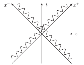
Figure 1: Light-front coordinates. The light wave along the $x^{-}$ axis is everywhere at one light-front time $x^{+}$.

Some work is done with definitions of $x^{\pm}$ that differ by a factor of $\sqrt{2}$. This shifts factors of 2 and 1/2 in what follows.

Spatial four-vectors are written as $x^{\mu}=(x^{+},x^{-},\vec{x}_{\perp})$ and light-front three-vectors as $\underline{x}=(x^{-},\vec{x}_{\perp})$. The conjugate four-momentum is $p^{\mu}=(p^{-},p^{+},\vec{p}_{\perp})$, with $p^{-}\equiv E-p_{z}$ the light-front energy and $p^{+}\equiv E+p_{z}$ the longitudinal light-front momentum. The light-front three-momentum is denoted $\underline{p}=(p^{+},\vec{p}_{\perp})$. The dot product of a coordinate vector and a momentum vector is $p\cdot x=\frac{1}{2}(p^{-}x^{+}+p^{+}x^{-})-\vec{p}_{\perp}\cdot\vec{x}_{\perp}$, hence the designations of $p^{-}$ and $p^{+}$ as light-front energy and momentum, conjugate to $x^{+}$ and $x^{-}$, respectively. The four-vector dot product implies the following spacetime metric

$$g_{\mu\nu}=\left(\begin{array}[]{cccc}0&1/2&0&0\\ 1/2&0&0&0\\ 0&0&-1&0\\ 0&0&0&-1\end{array}\right).$$ (2)

A dot product for light-front three-vectors is defined as $\underline{p}\cdot\underline{x}=\frac{1}{2}p^{+}x^{-}-\vec{p}_{\perp}\cdot\vec{x}_{\perp}$. The mass-shell condition $p^{2}=m^{2}$ becomes $p^{-}=(m^{2}+p_{\perp}^{2})/p^{+}$.

Spatial derivatives are defined by

$$\partial_{\pm}\equiv\frac{\partial}{\partial x^{\pm}}=\frac{1}{2}\left(\frac{\partial}{\partial t}\pm\frac{\partial}{\partial z}\right),\;\;\vec{\partial}_{\perp}\equiv\vec{\nabla}_{\perp}=\left(\frac{\partial}{\partial x},\frac{\partial}{\partial y}\right).$$ (3)

The factor of $\frac{1}{2}$ comes from the inversion, $t=\frac{1}{2}(x^{+}+x^{-})$, $z=\frac{1}{2}(x^{+}-x^{-})$.

For a system of $n$ particles, with $p_{i}$ the momentum of the $i$th particle and $M$ the invariant mass, we define the total momentum $P$ with components $P^{+}=\sum_{i}p_{i}^{+}$, $\vec{P}_{\perp}=\sum_{i}\vec{p_{i}}_{\perp}$, and $P^{-}=(M^{2}+P_{\perp}^{2})/P^{+}$. Notice, however, that, except for free particles, $P^{-}$ is not equal to $\sum_{i}p_{i}^{-}$; the momentum is not on the light-front energy shell.

It is convenient to define relative momenta for the constituents, as a longitudinal momentum fraction $x_{i}\equiv p_{i}^{+}/P^{+}$ and a relative transverse momentum $\vec{k_{i}}_{\perp}\equiv\vec{p_{i}}_{\perp}-x_{i}\vec{P}_{\perp}$. Clearly, the $x_{i}$ sum to unity and the $\vec{k_{i}}_{\perp}$ sum to zero. Also, if the total transverse momentum $\vec{P}_{\perp}$ is zero, the relative transverse momenta are just the transverse momenta, making this a convenient and frequent choice of frame.

Any two frames of reference can be connected by a combination of longitudinal boosts along $z$ and light-front transverse boosts that combine a transverse boost and a rotation. A longitudinal boost in equal-time coordinates is defined as

$$E^{\prime}=\gamma(E-\beta p_{z}),\;\;p^{\prime}_{z}=\gamma(p_{z}-\beta E),\;\;\vec{p^{\prime}}_{\perp}=\vec{p}_{\perp},$$ (4)

with $\beta$ the relative velocity and $\gamma=1/\sqrt{1-\beta^{2}}$. In terms of light-front coordinates, this boost is

$$p^{\prime-}=E^{\prime}-p^{\prime}_{z}=\sqrt{\frac{1+\beta}{1-\beta}}p^{-},\;\;p^{\prime+}=E^{\prime}+p^{\prime}_{z}=\sqrt{\frac{1-\beta}{1+\beta}}p^{+},\;\;\vec{p^{\prime}}_{\perp}=\vec{p}_{\perp},$$ (5)

The light-front transverse boost is

$$p^{\prime-}=p^{-}+2\vec{p}_{\perp}\cdot\vec{\beta}_{\perp}+\beta^{2}p^{+},\;\;p^{\prime+}=p^{+},\;\;\vec{p^{\prime}}_{\perp}=\vec{p}_{\perp}+p^{+}\vec{\beta}_{\perp},$$ (6)

where $\vec{\beta}_{\perp}=(\beta_{x},\beta_{y})$ is again the relative velocity. The relative momenta of constituents, $x_{i}$ and $\vec{k_{i}}_{\perp}$ are invariant with respect to these boosts. Therefore, wave functions constructed in terms of these variables will themselves be invariant. This separation of internal (relative) momenta and the external momentum is responsible for much of the utility of light-front quantization.

One disadvantage of light-front coordinates is the loss of explicit rotational symmetry. Except for rotations about the $z$ axis, rotations are associated with dynamical operators that include the interaction. This means that Fock states cannot be eigenstates of total angular momentum; the rotation operator changes the particle count. For some discussion of the restoration of rotational invariance, see [35].

2.2 Free Fields

2.2.1 scalar field

The Lagrangian for a free neutral scalar field $\phi$ of mass $m$ is

$${\cal L}=\frac{1}{2}(\partial_{\mu}\phi)^{2}-\frac{1}{2}m^{2}\phi^{2}=\frac{1}{2}\partial_{-}\phi\partial_{+}\phi-\frac{1}{2}(\vec{\partial}_{\perp}\phi)^{2}-\frac{1}{2}m^{2}\phi^{2}.$$ (7)

From this Lagrangian, we obtain the field equation as the Klein–Gordon equation, $\partial^{\mu}\partial_{\mu}\phi+m^{2}\phi=0$, and the conjugate momentum $\pi\equiv\delta{\cal L}/\delta(\partial_{+}\phi)=\frac{1}{2}\partial_{-}\phi$. Therefore, the Hamiltonian density for translations in light-front time $x^{+}$ is

$${\cal H}\equiv\pi\partial_{+}\phi-{\cal L}=\frac{1}{2}(\vec{\partial}_{\perp}\phi)^{2}+\frac{1}{2}m^{2}\phi^{2}.$$ (8)

The light-front Hamiltonian ${\cal P}^{-}$ is just the integral of this density (normal ordered) over the light-front spatial volume at $x^{+}=0$: ${\cal P}^{-}=\int d\underline{x}:{\cal H}(x^{+}=0):$, with $d\underline{x}=dx^{-}d^{2}x_{\perp}$.

The field equation is solved by the Fourier decomposition

$$\phi(x)=\int_{p^{+}\geq 0}\frac{dp^{+}}{\sqrt{4\pi p^{+}}}\frac{d^{2}p_{\perp}}{2\pi}\left[a(\underline{p})e^{-ip\cdot x}+a^{\dagger}(\underline{p})e^{ip\cdot x}\right],$$ (9)

with $p^{2}=m^{2}$. The range of integration is restricted to $p^{+}\geq 0$ because $p^{+}=\sqrt{m^{2}+p_{z}^{2}+\vec{p}_{\perp}^{2}}+p_{z}$ is always nonnegative. The $p^{+}$ and $\vec{p}_{\perp}$ integration factors are written separately, to make easy identification of the parts applicable to 1+1 and 3+1 dimensional theories. The creation and annihilation operators satisfy commutation relations

$${[}a(\underline{p}),a(\underline{p^{\prime}})]=0,\;\;{[}a^{\dagger}(\underline{p}),a^{\dagger}(\underline{p^{\prime}})]=0,\;\;{[}a(\underline{p}),a^{\dagger}(\underline{p^{\prime}})]=\delta(\underline{p}-\underline{p^{\prime}})\equiv\delta(p^{+}-p^{\prime+})\delta(\vec{p}_{\perp}-\vec{p^{\prime}}_{\perp}).$$ (10)

With use of the identity $\int dx^{-}\exp[i(k^{+}-q^{+})x^{-}/2]=4\pi\delta(k^{+}-q^{+})$, the light-front Hamiltonian can be reduced to

$${\cal P}^{-}=\int d\underline{p}\frac{m^{2}+\vec{p}_{\perp}^{2}}{p^{+}}a^{\dagger}(\underline{p})a(\underline{p}).$$ (11)

Clearly, this operator sums up the $p^{-}$ contributions identified by the number operator $a^{\dagger}(\underline{p})a(\underline{p})$ and therefore represents the light-front kinetic energy of the free field.

The case of the charged scalar is a slight generalization of the neutral case. The Lagrangian is

$${\cal L}=\partial_{\mu}\phi^{*}\partial^{\mu}\phi-m^{2}|\phi|^{2}.$$ (12)

The field equation is again the Klein–Gordon equation. The Hamiltonian density is

$${\cal H}=|\vec{\partial}_{\perp}\phi|^{2}+m^{2}|\phi|^{2}.$$ (13)

The field equation is solved by the Fourier decomposition

$$\phi(x)=\int\frac{dp^{+}d^{2}p_{\perp}}{\sqrt{16\pi^{3}p^{+}}}\left[c_{+}(\underline{p})e^{-ip\cdot x}+c_{-}^{\dagger}(\underline{p})e^{ip\cdot x}\right].$$ (14)

The nonzero commutation relations of the creation and annihilation operators are

$${[}c_{\pm}(\underline{p}),c_{\pm}^{\dagger}(\underline{p^{\prime}})]=\delta(\underline{p}-\underline{p^{\prime}}).$$ (15)

The normal-ordered light-front Hamiltonian can be reduced to

$${\cal P}^{-}=\int d\underline{p}\frac{m^{2}+\vec{p}_{\perp}^{2}}{p^{+}}\left[c_{+}^{\dagger}(\underline{p})c_{+}(\underline{p})+c_{-}^{\dagger}(\underline{p})c_{-}(\underline{p})\right].$$ (16)

2.2.2 fermion field

The Lagrangian for a free fermion field is

$${\cal L}=\overline{\psi}(i\gamma\cdot\partial-m)\psi,$$ (17)

where the $\gamma^{\mu}=(\gamma^{0},\vec{\gamma})=(\beta,\beta\vec{\alpha})$ are the Dirac matrices. One useful representation of these matrices is

$$\beta=\gamma^{0}=\left(\begin{array}[]{cc}I&0\\ 0&-I\end{array}\right),\;\;\vec{\alpha}=\left(\begin{array}[]{cc}0&\vec{\sigma}\\ \vec{\sigma}&0\end{array}\right),\;\;\vec{\gamma}=\left(\begin{array}[]{cc}0&\vec{\sigma}\\ -\vec{\sigma}&0\end{array}\right),$$ (18)

with $I$ the $2\times 2$ identity matrix and $\vec{\sigma}$ the Pauli matrices.

The field equation is the Dirac equation

$$(i\gamma\cdot\partial-m)\psi=0$$ (19)

The light-front gamma matrices are $\gamma^{\pm}\equiv\gamma^{0}\pm\gamma^{3}=(\gamma^{\mp})^{\dagger}$. They obey the usual anticommutation relation $\{\gamma^{\mu},\gamma^{\nu}\}=2g^{\mu\nu}$, with $g^{\mu\nu}$ the light-front metric. The Dirac equation can then be written as

$$(i\frac{1}{2}\gamma^{0}\gamma^{+}\partial_{+}+i\frac{1}{2}\gamma^{0}\gamma^{-}\partial_{-}+i\vec{\alpha}_{\perp}\cdot\vec{\partial}_{\perp}-\beta m)\psi=0.$$ (20)

With use of the projections $\Lambda_{\pm}\equiv\frac{1}{2}\gamma^{0}\gamma^{\pm}$, which satisfy

$$\Lambda_{\pm}^{2}=\Lambda_{\pm},\;\;\Lambda_{\pm}\Lambda_{\mp}=0,\;\;\Lambda_{+}+\Lambda_{-}=1,$$ (21)

the Dirac equation separates into a dynamical equation for $\psi_{+}\equiv\Lambda_{+}\psi$

$$i\partial_{+}\psi_{+}-(-i\vec{\alpha}_{\perp}\cdot\vec{\partial}_{\perp}+\beta m)\psi_{-}=0$$ (22)

and a constraint equation for $\psi_{-}\equiv\Lambda_{-}\psi$

$$i\partial_{-}\psi_{-}-(-i\vec{\alpha}_{\perp}\cdot\vec{\partial}_{\perp}+\beta m)\psi_{+}=0.$$ (23)

Plane-wave solutions are readily found. Let $\psi_{\pm}(x)=w_{\pm}(p)e^{-ip\cdot x}$, where $\Lambda_{\pm}w_{\pm}=w_{\pm}$. Then the dynamical and constraint equations become

$$p^{+}w_{-}-(\vec{\alpha}_{\perp}\cdot\vec{p}_{\perp}+\beta m)w_{+}=0,\;\;p^{-}w_{+}-(\vec{\alpha}_{\perp}\cdot\vec{p}_{\perp}+\beta m)w_{-}=0.$$ (24)

The constraint equation is solved, to yield $w_{-}=\frac{1}{p^{+}}(\vec{\alpha}_{\perp}\cdot\vec{p}_{\perp}+\beta m)w_{+}$. Substitution of this solution into the dynamical equation, combined with reduction of Dirac matrix products, leaves

$$p^{-}w_{+}-\frac{m^{2}+\vec{p}_{\perp}^{2}}{p^{+}}w_{+}=0$$ (25)

which is immediately satisfied by $p$ on the mass shell. The only condition that remains to be satisfied is $\Lambda_{+}w_{+}=w_{+}$. In other words, $w_{+}$ must be an eigenvector of the projection with eigenvalue 1.

In the Dirac representation of the $\gamma$-matrices, the projection matrix has the form

$$\Lambda_{+}=\frac{1}{2}\left(\begin{array}[]{cccc}1&0&1&0\\ 0&1&0&-1\\ 1&0&1&0\\ 0&-1&0&1\end{array}\right).$$ (26)

This matrix has two eigenvectors, both with eigenvalue $+1$,

$$\chi_{+\frac{1}{2}}=\frac{1}{\sqrt{2}}\left(\begin{array}[]{c}1\\ 0\\ 1\\ 0\end{array}\right),\;\;\chi_{-\frac{1}{2}}=\frac{1}{\sqrt{2}}\left(\begin{array}[]{c}0\\ 1\\ 0\\ -1\end{array}\right).$$ (27)

These can be used as a spinor basis for the Fourier expansion of the field $\psi_{+}$.

The solution of the Dirac equation for the dynamical field can then be written as

$$\psi_{+}(x)=\int\frac{d\underline{p}}{\sqrt{16\pi^{3}}}\sum_{s=\pm 1/2}\left[b_{s}(\underline{p})\chi_{s}e^{-ip\cdot x}+d_{s}^{\dagger}(\underline{p})\chi_{-s}e^{ip\cdot x}\right].$$ (28)

The nonzero anticommutators are

$$\{b_{s}(\underline{p}),b_{s^{\prime}}^{\dagger}(\underline{p}^{\prime})\}=\delta_{ss^{\prime}}\delta(\underline{p}-\underline{p^{\prime}}),\;\;\{d_{s}(\underline{p}),d_{s^{\prime}}^{\dagger}(\underline{p}^{\prime})\}=\delta_{ss^{\prime}}\delta(\underline{p}-\underline{p^{\prime}}).$$ (29)

The expansion for the constrained field $\psi_{-}$ is obtained by applying $(\vec{\alpha}_{\perp}\cdot\vec{p}_{\perp}+\beta m)/p^{+}$ to the expansion for $\psi_{+}$. The complete fermion field $\psi=\psi_{+}+\psi_{-}$ can then be simplified to

$$\psi(x)=\int\frac{d\underline{p}}{\sqrt{16\pi^{3}p^{+}}}\sum_{s=\pm 1/2}\left[b_{s}(\underline{p})u_{s}(\underline{p})e^{-ip\cdot x}+d^{\dagger}_{s}(\underline{p})v_{s}(\underline{p})e^{ip\cdot x}\right],$$ (30)

with

$$u_{s}(\underline{p})\equiv\frac{1}{\sqrt{p^{+}}}\left[p^{+}+\vec{\alpha}_{\perp}\cdot\vec{p}_{\perp}+\beta m\right]\chi_{s},\;\;v_{s}(\underline{p})\equiv\frac{1}{\sqrt{p^{+}}}\left[p^{+}+\vec{\alpha}_{\perp}\cdot\vec{p}_{\perp}-\beta m\right]\chi_{-s}.$$ (31)

The index $s$ is the light-front helicity, sometimes loosely called the spin (projection) and not to be confused with the ordinary (Jacob–Wick) helicity, the latter being the projection onto the equal-time three-momentum. The light-front helicity is left invariant by boosts that the leave the light front itself invariant.

In terms of the dynamical field, the Lagrangian is

$${\cal L}=i\psi_{+}^{\dagger}\partial_{+}\psi_{+}-\psi_{+}^{\dagger}(i\vec{\alpha}_{\perp}\cdot\vec{\partial}_{\perp}-\beta m)\frac{1}{i\partial_{-}}(i\vec{\alpha}_{\perp}\cdot\vec{\partial}_{\perp}-\beta m)\psi_{+},$$ (32)

where $\frac{1}{i\partial_{-}}$ appears as part of a formal solution of the constraint equation that eliminates $\psi_{-}$. The Hamiltonian density is

$${\cal H}=\psi_{+}^{\dagger}(i\vec{\alpha}_{\perp}\cdot\vec{\partial}_{\perp}-\beta m)\frac{1}{i\partial_{-}}(i\vec{\alpha}_{\perp}\cdot\vec{\partial}_{\perp}-\beta m)\psi_{+},$$ (33)

and the normal-ordered light-front Hamiltonian is

$${\cal P}^{-}=\int d\underline{p}\frac{m^{2}+\vec{p}_{\perp}^{2}}{p^{+}}\sum_{s}\left[b_{s}^{\dagger}(\underline{p})b_{s}(\underline{p})+d_{s}^{\dagger}(\underline{p})d_{s}(\underline{p})\right].$$ (34)

2.2.3 vector field

The Lagrangian of a free massive vector field is

$${\cal L}=-\frac{1}{4}F^{2}+\frac{1}{2}\mu A^{2}-\frac{1}{2}\zeta(\partial\cdot A)^{2},$$ (35)

where $\zeta$ is the gauge-fixing parameter and $F^{\mu\nu}=\partial^{\mu}A^{\nu}-\partial^{\nu}A^{\mu}$ is the field-strength tensor. The Lorentz gauge condition $\partial\cdot A=0$ is to be satisfied by a projection of states onto a physical subspace.

An alternative gauge choice [2] is light-cone gauge $A^{+}=0$. The $A^{-}$ component is then a constrained field and only the transverse components $\vec{A}_{\perp}$ are dynamical. Thus, the quantization has the advantage of requiring only physical fields with positive metric. However, there is the disadvantage that there is no gauge parameter with respect to which one might check gauge invariance (in the massless limit).

The Euler–Lagrange field equation for the Lorentz-gauge Lagrangian is

$$(\Box+\mu^{2})A_{\mu}-(1-\zeta)\partial_{\mu}(\partial\cdot A)=0.$$ (36)

The solution as a Fourier expansion can be constructed by the light-front analog [27] of a method due to Stueckelberg [36]. With the introduction of a four-momentum $\tilde{k}$ associated with a different mass $\tilde{\mu}\equiv\mu/\sqrt{\zeta}$, defined by

$$\underline{\tilde{k}}=\underline{k},\;\;\tilde{k}^{-}=(k_{\perp}^{2}+\tilde{\mu}^{2})/k^{+},$$ (37)

the expansion can be written as

$$A_{\mu}(x)=\int\frac{d\underline{k}}{\sqrt{16\pi^{3}k^{+}}}\left\{\sum_{\lambda=1}^{3}e_{\mu}^{(\lambda)}(\underline{k})\left[a_{\lambda}(\underline{k})e^{-ik\cdot x}+a_{\lambda}^{\dagger}(\underline{k})e^{ik\cdot x}\right]+e_{\mu}^{(0)}(\underline{k})\left[a_{0}(\underline{k})e^{-i\tilde{k}\cdot x}+a_{0}^{\dagger}(\underline{k})e^{i\tilde{k}\cdot x}\right]\right\},$$ (38)

with polarization vectors defined by

$$e^{(1,2)}(\underline{k})=(0,2\hat{e}_{1,2}\cdot\vec{k}_{\perp}/k^{+},\hat{e}_{1,2}),\;\;e^{(3)}(\underline{k})=((k_{\perp}^{2}-\mu^{2})/k^{+},k^{+},\vec{k}_{\perp})/\mu,\;\;e^{(0)}(\underline{k})=\tilde{k}/\mu.$$ (39)

The $\hat{e}_{1,2}$ are transverse unit vectors. These polarizations satisfy $k\cdot e^{(\lambda)}=0$ and $e^{(\lambda)}\cdot e^{(\lambda^{\prime})}=-\delta_{\lambda\lambda^{\prime}}$ for $\lambda,\lambda^{\prime}=1,2,3$. The first term in $A_{\mu}$ satisfies both $(\Box+\mu^{2})A_{\mu}=0$ and $\partial\cdot A=0$ separately. The $\lambda=0$ term violates each, but the violations cancel in the sum, which is the field equation. The nonzero commutators are

$$[a_{\lambda}(\underline{k}),a_{\lambda^{\prime}}^{\dagger}(\underline{k^{\prime}})]=\epsilon^{\lambda}\delta_{\lambda\lambda^{\prime}}\delta(\underline{k}-\underline{k^{\prime}}),$$ (40)

with $\epsilon^{\lambda}=(-1,1,1,1)$ the metric of each field component.

The light-front Hamiltonian density is

$${\cal H}=\frac{1}{2}\sum_{\mu=0}^{3}\epsilon^{\mu}\left[(\partial_{\perp}A^{\mu})^{2}+\mu^{2}(A^{\mu})^{2}\right]+\frac{1}{2}(1-\zeta)(\partial\cdot A)(\partial\cdot A-2\partial_{-}A^{-}-2\partial_{\perp}\cdot\vec{A}_{\perp}).$$ (41)

The first term is obviously the Feynman-gauge ($\zeta=1$) piece. The light-front Hamiltonian for the free massive vector field is then found to be

$${\cal P}^{-}=\int d\underline{k}\sum_{\lambda}\epsilon^{\lambda}\frac{k_{\perp}^{2}+\mu_{\lambda}^{2}}{k^{+}}a_{\lambda}^{\dagger}(\underline{k})a_{\lambda}(\underline{k}),$$ (42)

with $\mu_{\lambda}=\mu$ for $\lambda=1,2,3$, but $\mu_{0}=\tilde{\mu}$. Thus, the Hamiltonian for the free vector field takes the usual form except that the mass of the fourth polarization is different and gauge dependent and that the metric of this polarization is opposite that of the other polarizations. In Feynman gauge, this reduces to the usual Gupta–Bleuler quantization [37] with $\tilde{\mu}=\mu$.

2.3 Wave Functions

The light-front Hamiltonian eigenvalue problem is

$${\cal P}^{-}|\psi(\underline{P})\rangle=\frac{M^{2}+P_{\perp}^{2}}{P^{+}}|\psi(\underline{P})\rangle,\;\;\underline{\cal P}|\psi(\underline{P})\rangle=\underline{P}|\psi(\underline{P})\rangle.$$ (43)

The second equation is solved explicitly by expanding the eigenstate $|\psi(\underline{P})\rangle$ in Fock states with $n$ constituents with relative momenta $x_{i}$ and $\vec{k_{i}}_{\perp}$

$$|x_{i},\vec{k_{i}}_{\perp},\underline{P},n\rangle=\frac{1}{\sqrt{n!}}\prod_{i=1}^{n}a^{\dagger}(x_{i}P^{+},\vec{k_{i}}_{\perp}+x_{i}\vec{P}_{\perp})|0\rangle.$$ (44)

Here the construction is for scalar constituents of a single type, but the form is easily generalized.

The empty Fock vacuum $|0\rangle$ is an eigenstate of ${\cal P}^{-}$, even in the presence of interactions, with the possible exception of contributions from modes of zero $p^{+}$. This is because the longitudinal light-front momentum $p^{+}$ cannot be negative, and no interaction can create particles from the vacuum without violating momentum conservation. For practical calculations, this is an advantage of light-front quantization, in that massive eigenstates can be computed without first computing the vacuum state, and any Fock-state expansion for a massive state does not have spurious vacuum contributions. The latter aspect makes the Fock-state wave functions unambiguous as probability amplitudes for constituent momentum distributions. This does leave open the question of the connection with the equal-time vacuum and properties such as symmetry breaking that are usually associated with the vacuum [38, 39]; however, these considerations are beyond the scope of this review.

The Fock-state expansion for the eigenstate is

$$|\psi(\underline{P})\rangle=\sum_{n}(P^{+})^{\frac{n-1}{2}}\int\prod_{i}^{n}dx_{i}d^{2}k_{i\perp}\delta(1-\sum_{i}^{n}x_{i})\delta(\sum_{i}^{n}\vec{k_{i}}_{\perp})\psi_{n}(x_{i},\vec{k_{i}}_{\perp})|x_{i},\vec{k_{i}}_{\perp},\underline{P},n\rangle.$$ (45)

The $\psi_{n}$ are the Fock-state momentum-space wave functions for $n$ constituents. Substitution into the first equation of the eigenvalue problem yields a coupled set of integral equations for these wave functions, with the total mass $M$ as the eigenvalue. These equations and the wave functions are independent of the total momentum $\underline{P}$.

The normalization of the wave functions is determined by the requirement $\langle\psi(\underline{P^{\prime}})|\psi(\underline{P})\rangle=\delta(\underline{P^{\prime}}-\underline{P})$. Once the contractions of the creation and annihilation operators are carried out, this reduces to

$$1=\sum_{n}\int\prod_{i}^{n}dx_{i}d^{2}k_{i\perp}\delta(1-\sum_{i}^{n}x_{i})\delta(\sum_{i}^{n}\vec{k_{i}}_{\perp})|\psi_{n}(x_{i},\vec{k_{i}}_{\perp})|^{2}.$$ (46)

The individual terms in the sum over $n$ provide the probabilities for each Fock sector. The wave functions and their normalization are independent of $P^{+}$ because the factor of $(P^{+})^{\frac{n-1}{2}}$ in (45) has been arranged to cancel the factors of $1/P^{+}$ that come from the contractions

$$[a(x^{\prime}_{i^{\prime}}P^{\prime+},\vec{k^{\prime}_{i^{\prime}}}_{\perp}+x^{\prime}_{i^{\prime}}\vec{P^{\prime}}_{\perp}),a^{\dagger}(x_{i}P^{+},\vec{k_{i}}_{\perp}+x_{i}\vec{P}_{\perp})]=\delta(x^{\prime}_{i^{\prime}}P^{\prime+}-x_{i}P^{+})\delta(\vec{k^{\prime}_{i^{\prime}}}_{\perp}+x^{\prime}_{i^{\prime}}\vec{P^{\prime}}_{\perp}-\vec{k_{i}}_{\perp}-x_{i}\vec{P}_{\perp})$$ (47)

when integrated with respect to $x_{i}$.

For the free scalar, the equations decouple as simply

$$\left[\sum_{i}\frac{m^{2}+k_{i\perp}^{2}}{x_{i}}\right]\psi_{n}(x_{i},\vec{k_{i}}_{\perp})=M^{2}\psi_{n}(x_{i},\vec{k_{i}}_{\perp}).$$ (48)

This happens because

$$\sum_{i}\frac{m^{2}+(\vec{k_{i}}_{\perp}+x_{i}\vec{P}_{\perp})^{2}}{x_{i}P^{+}} = \frac{1}{P^{+}}\sum_{i}\left[\frac{m^{2}+k_{i\perp}^{2}+2x_{i}\vec{k_{i}}_{\perp}\cdot\vec{P}_{\perp}+x_{i}^{2}P_{\perp}^{2}}{x_{i}}\right]$$

$$= \frac{1}{P^{+}}\left[\sum_{i}\frac{m^{2}+k_{i\perp}^{2}}{x_{i}}+2\left(\sum_{i}\vec{k_{i}}_{\perp}\right)\cdot\vec{P}_{\perp}+\left(\sum_{i}x_{i}\right)P_{\perp}^{2}\right]$$

$$= \frac{1}{P^{+}}\left[\sum_{i}\frac{m^{2}+k_{i\perp}^{2}}{x_{i}}+P_{\perp}^{2}\right].$$

The last step follows from the momentum-conservation constraints $\sum_{i}\vec{k_{i}}_{\perp}=0$ and $\sum_{i}x_{i}=1$.

To make a connection with nonrelativistic quantum mechanics, consider the invariant mass $\sum_{i}(m^{2}+k_{i\perp}^{2})/x_{i}$ in the center of mass frame, where $P^{+}=M$ and $\vec{P}_{\perp}=0$. In this frame, $x_{i}=(\sqrt{m^{2}+\vec{k}_{i}^{2}}+k_{iz})/M$ and

$$\sum_{i}\frac{m^{2}+k_{i\perp}^{2}}{x_{i}}= = M\sum_{i}\frac{m^{2}+\vec{k}_{i}^{2}-k_{iz}^{2}}{\sqrt{m^{2}+\vec{k}_{i}^{2}}+k_{iz}}=mM\sum_{i}\frac{1+\vec{k}_{i}^{2}/m^{2}-k_{iz}^{2}/m^{2}}{\sqrt{1+\vec{k}_{i}^{2}/m^{2}}-k_{iz}/m}$$ (50)

$$\simeq mM\left(n-\sum_{i}\frac{k_{iz}}{m}+\sum_{i}\frac{\vec{k}_{i}^{2}}{2m^{2}}\right)=M\left(nm+\sum_{i}\frac{\vec{k}_{i}^{2}}{2m}\right).$$

Thus, the equation for the $n$-body wave function $\psi_{n}$ is approximately

$$\sum_{i}\frac{\vec{k}_{i}^{2}}{2m}\psi_{n}=(M-nm)\psi_{n}.$$ (51)

2.4 Observables

As in ordinary quantum mechanics, physical observables can be computed from matrix elements of appropriate operators with respect to chosen eigenstates. For example, the anomalous magnetic moment of the electron can be computed from the spin-flip matrix element of the electromagnetic current [40]. This is most conveniently done in the Drell–Yan frame [41], where the photon transfers zero longitudinal momentum. The electron itself is represented by a Fock-state expansion that includes dressing by photons and electron-positron pairs, as obtained from solving the Hamiltonian eigenvalue problem in QED. For the extension to generalized parton distributions [42], see the recent work of Chakrabarti et al. [43].

In general, the transition amplitude for absorption of a photon of momentum $q$ by a dressed electron is given by [44]

$$16\pi^{3}\langle\psi^{\sigma}(\underline{P}+\underline{q})|J^{+}(0)|\psi^{\pm}(\underline{P})\rangle=\bar{u}_{\sigma}(\underline{P}+\underline{q})\left[F_{1}(q^{2})+i\frac{\sigma^{\mu\nu}q_{\nu}}{2M}F_{2}(q^{2})\right]u_{\pm}(\underline{p}),$$ (52)

where $F_{1}$ and $F_{2}$ are the usual Dirac and Pauli form factors and $|\psi^{\sigma}(\underline{P})\rangle$ is the dressed electron state with light-front helicity $\sigma$. With $\vec{P}_{\perp}=0$, $q^{+}=0$, and $q^{-}=2q\cdot P/P^{+}$, the form factors can be obtained from [40]

$$F_{1}(q^{2})=\frac{16\pi^{3}}{2}\langle\psi^{\sigma}(\underline{P}+\underline{q})|J^{+}(0)|\psi^{\sigma}(\underline{P})\rangle$$ (53)

and

$$-\left(\frac{q_{x}-iq_{y}}{2M}\right)F_{2}(q^{2})=\frac{16\pi^{3}}{4\sigma}\langle\psi^{\sigma}(\underline{P}+\underline{q})|J^{+}(0)|\psi^{-\sigma}(\underline{P})\rangle.$$ (54)

Note that the factor of 1/2 comes from the normalization of the helicity spinors: $\bar{u}\gamma^{+}u=2p^{+}$. The plus component is used because, unlike the other components, it is not renormalized when the Fock space is truncated [44, 45]. The truncation destroys covariance, and the calculation of the other components requires great care [46].

The normal-ordered current operator $J^{+}$ is

$$J^{+}(0)=:\psi(0)^{\dagger}\gamma^{0}\gamma^{+}\psi(0):=2:\psi(0)^{\dagger}\Lambda_{+}\psi(0):=2:\psi_{+}(0)^{\dagger}\psi_{+}(0):,$$ (55)

which, on use of the mode expansion for $\psi_{+}$, simplifies to

$$J^{+}(0) = \int\frac{d\underline{p^{\prime}}}{\sqrt{16\pi^{3}}}\sum_{s^{\prime}=\pm 1/2}\int\frac{d\underline{p}}{\sqrt{16\pi^{3}}}\sum_{s=\pm 1/2}:\left[b_{s^{\prime}}^{\dagger}(\underline{p^{\prime}})\chi_{s^{\prime}}^{\dagger}+d_{s^{\prime}}(\underline{p^{\prime}})\chi_{-s}^{\dagger}\right]\left[b_{s}(\underline{p})\chi_{s}+d_{s}^{\dagger}(\underline{p})\chi_{-s}\right]:$$ (56)

$$= \int\frac{d\underline{p}d\underline{p^{\prime}}}{16\pi^{3}}\sum_{s=\pm 1/2}\left[b_{s}^{\dagger}(\underline{p^{\prime}})b_{s}(\underline{p})+b_{s}^{\dagger}(\underline{p^{\prime}})d_{-s}^{\dagger}(\underline{p})-d_{s}^{\dagger}(\underline{p})d_{s}(\underline{p^{\prime}})+d_{-s}(\underline{p^{\prime}})b_{s}(\underline{p})\right].$$ (57)

The last step required use of the orthonormality of $\chi_{s}$. With the current in this form, the utility of the $q^{+}=0$ frame becomes apparent; with no change in the longitudinal momentum, the pair creation and annihilation terms do not contribute and the current is diagonal in particle number.

Substitution of the final expression for the current and of the Fock-state expansion for the electron eigenstate into the matrix elements for the form factors leads to [40]

$$F_{1}(q^{2})=\sum_{n}\sum_{j}e_{j}\int\delta(1-\sum_{i}x_{i})\prod_{i}dx_{i}\delta(\sum_{i}\vec{k_{i}}_{\perp})\prod_{i}d^{2}k_{i\perp}\psi_{n}^{\sigma*}(x_{i},\vec{k}_{i\perp}^{\,\prime})\psi_{n}^{\sigma}(x_{i},\vec{k}_{i\perp})$$ (58)

and

$$-\left(\frac{q_{x}-iq_{y}}{2M}\right)F_{2}(q^{2})=\sum_{n}\sum_{j}e_{j}\int\delta(1-\sum_{i}x_{i})\prod_{i}dx_{i}\delta(\sum_{i}\vec{k_{i}}_{\perp})\prod_{i}d^{2}k_{i\perp}\psi_{n}^{1/2*}(x_{i},\vec{k}_{i\perp}^{\,\prime})\psi_{n}^{-1/2}(x_{i},\vec{k}_{i\perp}^{\,\prime}).$$ (59)

Here $\psi_{n}^{\sigma}$ is the $n$-body Fock-state wave function for the eigenstate with light-front helicity $\sigma$, $e_{j}$ is the fractional charge of the struck constituent, and $\vec{k^{\prime}_{i}}_{\perp}$ is

$$\vec{k^{\prime}_{i}}_{\perp}=\left\{\begin{array}[]{ll}\vec{k_{i}}_{\perp}-x_{i}\vec{q}_{\perp},&i\neq j\\ \vec{k_{j}}_{\perp}+(1-x_{j})\vec{q}_{\perp},&i=j.\end{array}\right.$$ (60)

As can be easily seen, the normalization of the eigenstate is equivalent to $F_{1}(0)=1$.

The anomalous moment is $a_{e}=F_{2}(0)$, which requires the taking of the limit to zero momentum transfer. As shown in [40], this limit can be expressed as

$$a_{e} = \mp M\sum_{n}\sum_{j}e_{j}\int\delta(1-\sum_{i}x_{i})\delta(\sum_{i}\vec{k_{i}}_{\perp})\left(\prod_{i}dx_{i}d^{2}k_{i\perp}\right)$$

$$\times\psi_{n}^{\pm*}(x_{i},\vec{k_{i}}_{\perp})\left[\sum_{i\neq j}x_{i}\left(\frac{\partial}{\partial k_{ix}}\pm i\frac{\partial}{\partial k_{iy}}\right)\right]\psi_{n}^{\mp}(x_{i},\vec{k_{i}}_{\perp}).$$

Thus, the anomalous moment can be computed given the solution to the coupled equations for the wave functions.

The Dirac form factor, or more specifically its slope at zero momentum transfer, can be used to measure the average radius of the eigenstate as $R=\sqrt{-6F^{\prime}_{1}(0)}$. The slope is obtained from the derivative of the expression for $F_{1}(q^{2})$, which can be simplified to

$$F^{\prime}_{1}(0)=\sum_{n}\sum_{j}\frac{e_{j}}{2}\int\delta(1-\sum_{i}x_{i})\prod_{i}dx_{i}\delta(\sum_{i}\vec{k_{i}}_{\perp})\prod_{i}d^{2}k_{i\perp}\sum_{i\neq j}|x_{i}\vec{\nabla_{i}}_{\perp}\psi_{n}^{\sigma}(x_{i},\vec{k}_{i\perp})|^{2}.$$ (62)

The finite temperature properties of a theory can computed from the partition function $Z=e^{-E/T}$. One does not use the light-front analog $e^{-P^{-}/T_{\rm LF}}$ because it does not correspond to a heat bath at rest [48]. Other examples of where this choice matters can be found in the variational analysis of $\phi^{4}$ theory [49] and the light-front derivation of the Casimir effect [15, 50, 51]. This is not to say that light-front quantization cannot be used; the physics should be the same in any coordinate system.

To compute the partition function, one needs the spectrum of the theory, which is what nonperturbative light-front methods can yield. Each mass eigenstate contributes according to its ordinary energy $E$. For bosonic states of mass $M_{n}$ in one space dimension this yields a free-energy contribution of [52]

$$F_{B}=\frac{VT}{\pi}\sum_{n=1}^{\infty}\int_{M_{n}}^{\infty}dp_{0}\frac{p_{0}}{\sqrt{p_{0}^{2}-M_{n}^{2}}}\ln\left(1-e^{-p_{0}/T}\right)$$ (63)

in a volume $V$. For fermions the contribution is

$$F_{F}=-\frac{VT}{\pi}\sum_{n=1}^{\infty}\int_{M_{n}}^{\infty}dp_{0}\frac{p_{0}}{\sqrt{p_{0}^{2}-M_{n}^{2}}}\ln\left(1+e^{-p_{0}/T}\right).$$ (64)

In supersymmetric theories, the bosonic and fermionic mass spectra are the same, and we can readily combine these expressions to obtain the total free energy

$$F(T,V)=-(K-1)\pi VT^{2}-\frac{2VT}{\pi}\sum_{n=1}^{\infty}{\sum_{l=0}^{\infty}}M_{n}\frac{K_{1}\left((2l+1)\frac{M_{n}}{T}\right)}{(2l+1)}.$$ (65)

Here the logarithms have been expanded, the integral over $p_{0}$ performed, and the contribution of $K-1$ zero-mass states separated explicitly. The sum over $l$ is well approximated by the first few terms. The sum over $n$ can be represented by an integral over a density of states $\int\rho(M)dM$. The density can be approximated by a continuous function that is fit to the numerical spectrum, and the integral $\int dM$ computed by standard numerical techniques.

Additional work on finite-temperature physics on the light front has been done by Beyer and Strauss. They studied both two-dimensional QED [53] and the Nambu-Jona-Lasinio model [54].

3 Methods of Calculation

3.1 Discretized Light-Cone Quantization

One very systematic approach to solving a quantum field theory nonperturbatively is that of discretized light-cone quantization (DLCQ) [12, 55]. It has had particular utility in two dimensions. This includes calculations of eigenstates in supersymmetric Yang–Mills theories [56] and $\phi^{4}$ theory [57, 58, 59, 60, 61], as well as the early applications to Yukawa theory [12], $\phi^{3}$ and $\phi^{4}$ theories [62, 63, 64], QED [65], and QCD [66].

Although DLCQ is in a sense a trapezoidal approximation to the coupled integral equations for the wave functions, it is based on quantization in a discrete basis obtained by placing the system in a light-front box

$$-L<x^{-}<L\,,\;\;-L_{\perp}<x,y<L_{\perp}.$$ (66)

For bosons, periodic boundary conditions are used and for fermions, antiperiodic, leading to discrete momenta

$$p^{+}\rightarrow\frac{\pi}{L}n\,,\;\;\vec{p}_{\perp}\rightarrow(\frac{\pi}{L_{\perp}}n_{x},\frac{\pi}{L_{\perp}}n_{y})\,,$$ (67)

with $n$ even for bosons and odd for fermions. Integrals are then replaced by discrete sums obtained as trapezoidal approximations on the grid of momentum values. For a generic integral, this takes the form

$$\int dp^{+}\int d^{2}p_{\perp}f(p^{+},\vec{p}_{\perp})\simeq\frac{2\pi}{L}\left(\frac{\pi}{L_{\perp}}\right)^{2}\sum_{n}\sum_{n_{x},n_{y}=-N_{\perp}}^{N_{\perp}}f(n\pi/L,\vec{n}_{\perp}\pi/L_{\perp}).$$ (68)

The sum on $n$ is restricted by the integer resolution [12]

$$K\equiv\frac{L}{\pi}P^{+},$$ (69)

with $K$ even for a boson eigenstate and odd for a fermion. The index $n$ can be no larger than this because all longitudinal momenta are positive, and the maximum individual momentum can then be no more than the total. The sums on $n_{x}$ and $n_{y}$ have been truncated at $\pm N_{\perp}$, with $N_{\perp}$ typically determined by a cutoff on the transverse momentum, either directly or as a cutoff on the invariant mass.

The longitudinal momentum fractions $x_{i}$ become ratios of integers $n_{i}/K$. Because the $n_{i}$ are all positive, DLCQ automatically limits the number of particles to be no more than $\sim\!\!K/2$. An explicit truncation in particle number, the light-front equivalent of the Tamm–Dancoff approximation [67], can also be made.

The limit $L\rightarrow\infty$ can be exchanged for the limit $K\rightarrow\infty$. This is because the combination of momentum components that defines ${\cal P}^{-}$ is simply proportional to $L$, so that the combination $P^{+}{\cal P}^{-}$, which has eigenvalues in the form $M^{2}+P_{\perp}^{2}$, is independent of $L$. As $K$ is increased, the longitudinal momentum is sampled at higher resolution.

The mode expansion for the quantum field is also approximated by a discrete sum. For example, the neutral scalar field becomes

$$\phi(x^{+}=0)=\frac{\pi}{L_{\perp}}\sum_{\underline{n}}\frac{1}{\sqrt{8\pi^{3}n}}\left[a(\underline{n})e^{-i\pi nx^{-}/2L+i\pi\vec{n}_{\perp}\cdot\vec{x}_{\perp}/L_{\perp}}+a^{\dagger}(\underline{n})e^{i\pi nx^{-}/2L-i\pi\vec{n}_{\perp}\cdot\vec{x}_{\perp}/L_{\perp}}\right],$$ (70)

with $\underline{n}=(n,n_{x},n_{y})$ and the creation operator for discrete momenta defined by

$$a^{\dagger}(\underline{n})=\frac{\pi}{L_{\perp}}\sqrt{\frac{2\pi}{L}}a^{\dagger}(\underline{p}).$$ (71)

It then satisfies a simple commutation relation

$$\left[a(\underline{n}),a^{\dagger}(\underline{n}^{\prime})\right]=\delta_{\underline{n^{\prime}},\underline{n}}\equiv\delta_{n^{\prime}n}\delta_{n^{\prime}_{x}n_{x}}\delta_{n^{\prime}_{y}n_{y}},$$ (72)

which follows from the continuum commutation relation and the discrete delta-function representation

$$\delta(\underline{p}-\underline{p}^{\prime})=\frac{L}{2\pi}\left(\frac{L_{\perp}}{\pi}\right)^{2}\delta_{\underline{n^{\prime}},\underline{n}}\,.$$ (73)

The discrete approximation of the eigenstate, with $P^{+}=K\pi/L$, $\vec{P}_{\perp}=0$, and $\underline{K}\equiv(K,\vec{0}_{\perp})$, is then

$$|\psi(\underline{K})\rangle=\sum_{n}\prod_{i}^{n}\sum_{\underline{n_{i}}}\delta_{\underline{K},\sum_{i}\underline{n_{i}}}\psi_{n}(\underline{n_{i}})|\underline{n_{i}},n\rangle,$$ (74)

where the discrete Fock states are

$$|\underline{n_{i}},n\rangle=\frac{1}{\sqrt{n!}}\prod_{i=1}^{n}a^{\dagger}(\underline{n_{i}})|0\rangle$$ (75)

and the discrete wave functions are related to the continuum wave functions by

$$\psi_{n}(\underline{n_{i}})=\left(\frac{K}{2}\frac{\pi^{2}}{L_{\perp}^{2}}\right)^{(n-1)/2}\psi_{n}(n_{i}/K,\vec{n}_{\perp}\pi/L_{\perp}).$$ (76)

The discrete eigenstate is normalized as $\langle\psi(\underline{K})|\psi(\underline{K})\rangle=1$, and the wave functions as

$$1=\sum_{n}\prod_{i}^{n}\sum_{\underline{n_{i}}}\delta_{\underline{K},\sum_{i}\underline{n_{i}}}|\psi_{n}(\underline{n_{i}})|^{2}.$$ (77)

Although the Fock basis is a natural way to write the eigenstate, a more convenient basis for a numerical calculation is the number basis, which eliminates summations over states that differ only by rearrangement of bosons of the same type.

There are zero modes, modes with zero longitudinal momentum. In DLCQ these are not dynamical but instead constrained by the spatial average of the Euler–Lagrange field equation [55, 68, 69]. These zero modes are usually either neglected or excluded by the choice of antiperiodic boundary conditions. This neglect does, however, slow convergence of the numerical solution, because contributions of order $1/K$ have been dropped; these are to be compared with the nominal $1/K^{2}$ errors associated with the trapezoidal approximation. For theories with symmetry breaking, the neglect can have serious consequences for the understanding of vacuum effects [68, 69, 70, 71, 72]. When included, zero modes generate effective interactions in the DLCQ Hamiltonian [73, 74, 75]. These effective interactions are typically due to end-point corrections where, although the wave function goes to zero as $x_{i}$ goes to zero, it does so slowly enough that the integral has a nonzero contribution which is missed by DLCQ’s neglect of the $x_{i}=0$ points in its trapezoidal approximation. They can be computed by solving the constraint equation, either nonperturbatively [71] or as an expansion in powers of $1/K$ [75]. There can also be quantum corrections to the constraint equation, such as contributions from zero-mode loops [76, 77].

If the transverse cutoff, such as an invariant-mass cutoff, creates a domain of integration that is not commensurate with the transverse DLCQ grid, there are errors generated if the basic DLCQ approximation is used. There is a truncation error, where the edge of the domain is not properly included, and there can be a loss of rotational symmetry. These can make the dependence on $K$ and $N_{\perp}$ very erratic and delay numerical convergence. However, these difficulties can be overcome by improvements on the trapezoidal approximation at the edge of the integration [78]. This idea also opens the possibility of using integration schemes that are more accurate than a trapezoidal rule for the entire domain; Simpson’s rule can be particularly helpful.

In general, any quadrature scheme that uses equally spaced points can be introduced. These will place unequal weighting factors inside the discrete sums. For the trapezoidal rule, the weighting factors are all the same (except for the neglected end points) and did not need to be considered beyond an overall factor of $1/K$. The unequal weights will destroy the symmetry of the matrix representing the action of ${\cal P}^{-}$; however, this symmetry can be restored by a simple rescaling. An eigenvalue problem of the form $\sum_{j}A_{ij}w_{j}u_{j}=\xi u_{i}$ can be rewritten as

$$\sum_{j}\sqrt{w_{i}w_{j}}A_{ij}\sqrt{w_{j}}u_{j}=\xi\sqrt{w_{i}}u_{i},$$ (78)

with $\sqrt{w_{i}w_{j}}A_{ij}$ the new symmetric matrix.

The term ‘DLCQ’ is sometimes extended to include quadratures that use unequally spaced points to approximate the coupled integral equations. This is at odds with the full intent of the DLCQ method, which discretizes before quantization, a process that would not admit unequally spaced points without spoiling momentum conservation for processes with more than two particles. Thus, the interaction terms of the DLCQ Hamiltonian could not be resolved into products of discrete creation and annihilation operators.

Nevertheless, quadratures with unequally spaced points can be a powerful tool [79, 80, 81, 82], even though their utility is limited to two-body equations. This is because the integral equations truncated at three-body contributions can usually be reduced to an effective equation in the two-body sector, sometimes without approximation and certainly when interactions are ignored in the three-body sector. The one-body and three-body wave functions are simply eliminated in favor of expressions relating them to the two-body wave function, which are then substituted into the original two-body equation. The use of unequally spaced quadratures for truncations beyond three constituents is best done by first introducing basis-function expansions, as discussed below in Sec. 3.4.

Quadratures with unequally spaced points can be particularly important when PV regularization is used, because the structure of the integrands in the effective equations can be such as to require very high resolution near the endpoints, inversely proportional to the PV mass squared [81]. In DLCQ such resolution would necessitate extremely large values of $K$, making the calculation intractable.

3.2 Supersymmetric Discretized Light-Cone Quantization

The supersymmetric form of DLCQ (SDLCQ) [33] is specifically designed to maintain supersymmetry in the discrete approximation. Ordinary DLCQ violates supersymmetry by terms that do not survive the continuum limit [83]. The SDLCQ construction discretizes the supercharge $Q^{-}$ and defines the Hamiltonian ${\cal P}^{-}$ by the superalgebra relation ${\cal P}^{-}=\{Q^{-},Q^{-}\}/2\sqrt{2}$. The range of transverse momentum is limited by a simple cutoff in the momentum value. The effects of zero modes cancel between bosonic and fermionic contributions, which enter with opposite signs [84].

The work done with SDLCQ typically uses the slightly different definition of light-front coordinates, with division by $\sqrt{2}$. The time coordinate is $x^{+}=(t+z)/\sqrt{2}$, and the space coordinate is $x^{-}\equiv(t-z)/\sqrt{2}$. The conjugate variables are the light-front energy $p^{-}=(E-p_{z})/\sqrt{2}$ and momentum $p^{+}\equiv(E+p_{z})/\sqrt{2}$. The mass-shell condition $p^{2}=m^{2}$ then yields $p^{-}=\frac{m^{2}+p_{\perp}^{2}}{2p^{+}}$; notice the factor of 2 in the denominator.

For example, consider supersymmetric QCD (SQCD) with a Chern–Simons (CS) term in the large-$N_{c}$ approximation [85]. The action is

$$S = \int d^{3}x\mbox{Tr}\left\{-\frac{1}{4}F_{\mu\nu}F^{\mu\nu}+D_{\mu}\xi^{\dagger}D^{\mu}\xi+i{\bar{\Psi}}D_{\mu}\Gamma^{\mu}\Psi\right.$$ (79)

$$\left.-g\left[{\bar{\Psi}}\Lambda\xi+\xi^{\dagger}{\bar{\Lambda}}\Psi\right]+\frac{i}{2}{\bar{\Lambda}}\Gamma^{\mu}D_{\mu}\Lambda+\frac{\kappa}{2}\epsilon^{\mu\nu\lambda}\left[A_{\mu}\partial_{\nu}A_{\lambda}+\frac{2i}{3}gA_{\mu}A_{\nu}A_{\lambda}\right]+\kappa\bar{\Lambda}\Lambda\right\}.$$

The adjoint fields are the gauge boson $A_{\mu}$ (gluons) and a Majorana fermion $\Lambda$ (gluinos); the fundamental fields are the Dirac fermion $\Psi$ (quarks) and a complex scalar $\xi$ (squarks). The CS coupling $\kappa$ induces a mass for the adjoint fields without breaking the supersymmetry; this inhibits formation of the long strings characteristic of super Yang–Mills theory. The covariant derivatives are

$$D_{\mu}\Lambda=\partial_{\mu}\Lambda+ig[A_{\mu},\Lambda]\,,\;\;D_{\mu}\xi=\partial_{\mu}\xi+igA_{\mu}\xi,\;\;D_{\mu}\Psi=\partial_{\mu}\Psi+igA_{\mu}\Psi.$$ (80)

The action is invariant under the following supersymmetry transformations, which are parameterized by a two-component Majorana fermion $\varepsilon$:

$$\delta A_{\mu}=\frac{i}{2}{\bar{\varepsilon}}\Gamma_{\mu}\Lambda,\;\;\delta\Lambda=\frac{1}{4}F_{\mu\nu}\Gamma^{\mu\nu}\varepsilon,\;\;\delta\xi=\frac{i}{2}{\bar{\varepsilon}}\Psi,\;\;\delta\Psi=-\frac{1}{2}\Gamma^{\mu}\varepsilon D_{\mu}\xi.$$ (81)

The supercharge associated with the corresponding Noether current is

$${\bar{\varepsilon}}Q = \int dx^{-}dx^{2}\left(\frac{i}{4}{\bar{\varepsilon}}\Gamma^{\alpha\beta}\Gamma^{+}\mbox{tr}\left(\Lambda F_{\alpha\beta}\right)+\frac{i}{2}D_{-}\xi^{\dagger}\ {\bar{\varepsilon}}\Psi+\frac{i}{2}\xi^{\dagger}{\bar{\varepsilon}}\Gamma^{+\nu}D_{\nu}\Psi\right.$$ (82)

$$-\left.\frac{i}{2}{\bar{\Psi}}\varepsilon D^{+}\xi+\frac{i}{2}D_{\nu}{\bar{\Psi}}\Gamma^{+\nu}\varepsilon\xi\right)\,.$$

In order that the Majorana fermion $\Lambda$ can be chosen real, the following representation is used for the Dirac matrices in three dimensions:

$$\gamma^{0}=\sigma_{2},\;\;\gamma^{1}=i\sigma_{1},\;\;\gamma^{2}=i\sigma_{3},$$ (83)

The fermionic spinor fields and the supercharge in terms of components are

$$\Lambda=\left(\lambda,{\tilde{\lambda}}\right)^{T}\,,\qquad\Psi=\left(\psi,{\tilde{\psi}}\right)^{T}\,,\qquad Q=\left(Q^{+},Q^{-}\right)^{T}\,.$$ (84)

The superalgebra has the form

$$\{Q^{+},Q^{+}\}=2\sqrt{2}P^{+}\,,\qquad\{Q^{-},Q^{-}\}=2\sqrt{2}P^{-}\,,\qquad\{Q^{+},Q^{-}\}=-4P_{\perp}\,.$$ (85)

The supercharge $Q^{-}$ is then discretized, and ${\cal P}^{-}$ is constructed from the superalgebra relation.

The eigenstates of ${\cal P}^{-}$ are of two types: meson-like states

$${\bar{f}}^{\dagger}_{i_{1}}(\underline{k}_{1})a^{\dagger}_{i_{1}i_{2}}(\underline{k}_{2})\dots b^{\dagger}_{i_{n}i_{n+1}}(\underline{k}_{n-1})\dots f^{\dagger}_{i_{p}}(\underline{k}_{n})|0\rangle,$$ (86)

where $f^{\dagger}=$ creates a quark or squark, $a^{\dagger}$ creates a gluon, and $b^{\dagger}$ creates a gluino; and glueball states

$${\rm Tr}[a^{\dagger}_{i_{1}i_{2}}(k_{1})\dots b^{\dagger}_{i_{n}i_{n+1}}(k_{n})]|0\rangle.$$ (87)

Because of the supersymmetry, either could be a boson or a fermion. In the large-$N_{c}$ limit, there is no mixing between these states, and they are composed of single traces. This simplifies the calculation, particularly with respect to the size of the matrices that need to be diagonalized. In general, states could be formed from multiple traces, such as

$${\rm Tr}[a^{\dagger}_{i_{1}i_{2}}(k_{1})\dots b^{\dagger}_{i_{n}i_{n+1}}(k_{n})]{\rm Tr}[a^{\dagger}_{j_{1}j_{2}}(p_{1})\dots b^{\dagger}_{j_{n}j_{n+1}}(p_{n})]\cdots|0\rangle,$$ (88)

which would lead to much larger SDLCQ matrix representations.

In addition to calculations of spectra, the SDLCQ approach can be used to calculate matrix elements, including correlators. Consider the (1+1)-dimensional stress-energy correlation function

$$F(x^{-},x^{+})\equiv\langle T^{++}(x)T^{++}(0)\rangle,$$ (89)

where $T^{\mu\nu}$ is the stress-energy tensor. For the string theory corresponding to two-dimensional ${\cal N}$=(8,8) SYM theory, $F$ can be calculated on the string-theory side in a weak-coupling super-gravity approximation. Its behavior for intermediate separations $r\equiv\sqrt{2x^{+}x^{-}}$ is [86, 87]

$$F(x^{-},x^{+})=\frac{N_{c}^{\frac{3}{2}}}{g_{\rm YM}r^{5}}.$$ (90)

In the SDLCQ approximation, this can be computed from SYM theory and compared.

With the total momentum $P^{+}=P_{-}$ fixed, the Fourier transform can be expressed in a spectral decomposed form as [86]

$$\tilde{F}(P_{-},x^{+}) = \frac{1}{2L}\langle T^{++}(P_{-},x^{+})T^{++}(-P_{-},0)\rangle$$

$$= \sum_{i}\frac{1}{2L}\langle 0|T^{++}(P_{-},0)|i\rangle e^{-iP^{i}_{+}x^{+}}\langle i|T^{++}(-P_{-},0)|0\rangle.$$

The position-space form is recovered by the inverse transform, with respect to $P_{-}=K\pi/L$. The continuation to Euclidean space is made by taking $r$ to be real. This yields

$$F(x^{-},x^{+})=\sum_{i}\Big{|}\frac{L}{\pi}\langle 0|T^{++}(K)|i\rangle\Big{|}^{2}\left(\frac{x^{+}}{x^{-}}\right)^{2}\frac{M_{i}^{4}K_{4}(M_{i}\sqrt{2x^{+}x^{-}})}{8\pi^{2}K^{3}}.$$ (92)

The stress-energy operator $T^{++}$ is

$$T^{++}(x^{-},x^{+})={\rm Tr}\left[(\partial_{-}X^{I})^{2}+\frac{1}{2}(iu^{\alpha}\partial_{-}u^{\alpha}-i(\partial_{-}u^{\alpha})u^{\alpha})\right].$$ (93)

In terms of the discretized creation operators, this becomes

$$T^{++}(-K)|0\rangle=\frac{\pi}{2L}\sum_{k=1}^{K-1}\left[-\sqrt{k(K-k)}a^{\dagger}_{Iij}(K-k)a^{\dagger}_{Iji}(k)+\left(\frac{K}{2}-k\right)b^{\dagger}_{\alpha ij}(K-k)b^{\dagger}_{\alpha ji}(k)\right]|0\rangle,$$ (94)

with sums over $i$ and $j$ implied. Thus $(L/\pi)\langle 0|T^{++}(K)|i\rangle$ is independent of $L$. Also, only one symmetry sector contributes.

The correlator behaves like $1/r^{4}$ at small $r$, as can be seen by taking the limit to obtain

$$\left(\frac{x^{-}}{x^{+}}\right)^{2}F(x^{-},x^{+})\sim\frac{N_{c}^{2}(2n_{b}+n_{f})}{4\pi^{2}r^{4}}(1-1/K).$$ (95)

To simplify the appearance of this behavior, $F$ can be rescaled by defining

$$f\equiv\langle T^{++}(x)T^{++}(0)\rangle\left(\frac{x^{-}}{x^{+}}\right)^{2}\frac{4\pi^{2}r^{4}}{N_{c}^{2}(2n_{b}+n_{f})}.$$ (96)

Then $f$ is just $(1-1/K)$ for small $r$.

The function $f$ can be computed numerically for small matrix representations by obtaining the entire spectrum and for large representations by using Lanczos iterations. The Lanczos technique [88] (see Sec. 3.3) generates an approximate tridiagonal representation of the Hamiltonian which captures the important contributions after only a few iterations and which is easily diagonalized to compute the sum over eigenstates. For the correlator, this sum is weighted by the square of the projection $\langle i|T^{++}(-K)|0\rangle$. The Lanczos diagonalization algorithm will naturally generate the states with nonzero projection if $T^{++}(-K)|0\rangle$ is used as the initial vector for the iterations.

3.3 Lanczos Algorithm

The matrix approximations to the coupled integral equations for the wave functions are typically quite large and sparse. Standard diagonalization algorithms do not apply, because they require storage of the entire matrix, zeros and all, which is well beyond the capacity of current memory technology. However, there exist alternative algorithms that rely upon only an ability to multiply the matrix with a vector, something which can be done with relative ease for a matrix stored in a compressed form that strips away the zeros [90]. These algorithms generate better and better approximations to eigenvalues and eigenvectors by iteration, typically converging first to the largest and smallest eigenvalues. The best known of these algorithms is the Lanczos algorithm [88], which actually predates the current standard algorithms.

The basic Lanczos algorithm for the matrix eigenvalue problem $A\vec{\psi}_{\lambda}=\lambda\vec{\psi}_{\lambda}$, with $A$ Hermitian, is as follows. Set $\vec{u}_{1}$ to some normalized initial guess and set $b_{0}=0$. Then construct a sequence of normalized vectors $\vec{u}_{n}$ according to the iteration

$$b_{n}\vec{u}_{n+1}=A\vec{u}_{n}-a_{n}\vec{u}_{n}-b_{n-1}\vec{u}_{n-1},$$ (97)

with $a_{n}=\vec{u}_{n}^{*}\cdot A\vec{u}_{n}$ and $b_{n}$ chosen to normalize $\vec{u}_{n+1}$. The $\vec{u}_{n}$ form an orthonormal basis with respect to which $A$ is tridiagonal

$$A\rightarrow T\equiv\left(\begin{array}[]{llllll}a_{1}&b_{1}&0&0&0&\ldots\\ b_{1}&a_{2}&b_{2}&0&0&\ldots\\ 0&b_{2}&a_{3}&b_{3}&0&\ldots\\ 0&0&b_{3}&.&.&\ldots\\ 0&0&0&.&.&\ldots\\ .&.&.&.&.&\ldots\end{array}\right)\,.$$ (98)

The real symmetric matrix $T$ is easily diagonalized by ordinary means. The eigenvalues $\lambda_{k}$ of $T$ approximate the eigenvalues of $A$, and the eigenvectors $\vec{c}_{k}$ of $T$ can be used to construct approximate eigenvectors of $A$

$$\vec{\psi}_{\lambda_{k}}=\sum_{n}c_{kn}\vec{u}_{n}.$$ (99)

The only use of $A$ is in the multiplication of $A$ times $\vec{u}_{n}$. Generating a complete basis by iteration can yield the exact answer; however, doing many fewer iterations, even 20, can be sufficient to capture the extreme eigenvalues. If $\vec{u}_{n+1}$ is zero, the process terminates naturally, with $T$ an exact representation of $A$ in the subspace spanned by the eigenvectors with nonzero projection on $\vec{u}_{1}$.

A slightly altered form of the algorithm minimizes the storage requirements

$$\vec{v}_{n+1} = A\vec{u}_{n}-b_{n-1}\vec{u}_{n-1},\;\;a_{n}=\vec{v}_{n+1}^{*}\cdot\vec{u}_{n},\;\;\vec{v}_{n+1}^{\,\prime}=\vec{v}_{n+1}-a_{n}\vec{u}_{n},$$ (100)

$$b_{n} = \sqrt{\vec{v}_{n+1}^{\,\prime*}\cdot\vec{v}_{n+1}^{\,\prime}},\;\;\vec{u}_{n+1}=\vec{v}_{n+1}^{\,\prime}/b_{n}.$$ (101)

In this form, the vectors $\vec{u}_{n-1}$, $\vec{v}_{n+1}$, $\vec{v}_{n+1}^{\,\prime}$, and $\vec{u}_{n+1}$ can all be stored in the same array. Therefore, storage is required for only two vectors at a time, this sequence of overwritten vectors and $\vec{u}_{n}$. To be able to construct the eigenvectors of $A$, the vectors $\vec{u}_{n}$ do need to be saved for all $n$, written temporarily to disk and retrieved later, or the Lanczos algorithm can be run a second time, after the diagonalization of $T$, to accumulate the desired eigenvectors as each $\vec{u}_{n}$ is regenerated. During the second pass of the algorithm, the $a_{n}$ and $b_{n}$ are already known and do not need to be recalculated.

As simple as this all seems, there are limitations. Because all of the vectors $\vec{u}_{n}$ are generated by applying powers of $A$ to $\vec{u}_{1}$, only those eigenvectors with nonzero projections on $\vec{u}_{1}$ should appear. Depending on the application, this may actually be an advantage; however, for a generic diagonalization, it may be necessary to generate the initial guess with random components and/or run the algorithm more than once with different initial vectors.

Another limitation, which can be quite severe, is that round-off errors will eventually destroy the orthogonality of the Lanczos vectors $\vec{u}_{n}$. This will allow additional copies of the eigenvectors of $A$ to creep into the calculation. The eigenvalues of $T$ then include multiple copies of eigenvalues of $A$, a false degeneracy.

Various strategies have been developed to overcome this limitation. One is to re-orthogonalize the vectors as they are generated; however, this consumes time and storage. Another is to simply accept the copies; the eigenvalues are not wrong, but their degeneracy is unknown. This is not as bad as it sounds, since a correct estimate of any degeneracy is difficult in any case, because any symmetry in the initial vector will suppress degenerate eigenvectors with different symmetry, and multiple initial vectors will be needed to determine the degeneracy. A third approach is to restart the algorithm after a few iterations, using the best found estimate of the target eigenvector as the initial guess for the next set of iterations. A fourth strategy is to continue the iterations without re-orthogonalization but then detect and ignore the ‘ghost’ copies. The ghost copies can be detected by comparing the eigenvalues of the matrix obtained from $T$ by deleting the first row and first column [91]; any eigenvalue that appears in both lists is spurious.

Convergence of the algorithm can be monitored by measuring directly the convergence of the desired eigenvalue and by checking an estimate of the error in the eigenvalue, given by [91] $|b_{n}c_{kn}|$, where $n$ is the number of Lanczos iterations and $k$ is the index of the desired eigenvalue of $T$. If the error estimate begins to grow, the iterations should be restarted from the last best approximation to the eigenvector.

When PV regularization is used, the matrix representation has an indefinite metric. This could be handled with the biorthogonal version of the Lanczos algorithm [92]; however, a specialized form is much more efficient. Let $\eta$ represent the metric signature, so that numerical dot products are written as ${\vec{\phi}}^{\,\prime*}\cdot\eta{\vec{\phi}}$. The Hamiltonian matrix $A$ is not Hermitian but is self-adjoint with respect to this metric [93] $\eta^{-1}A^{\dagger}\eta=A$. The Lanczos algorithm for the diagonalization of $H$ then takes the form [94]

$$\alpha_{j} = \nu_{j}{\vec{q}}_{j}^{\,*}\cdot\eta H{\vec{q}}_{j},\;\;{\vec{r}}_{j}=H{\vec{q}}_{j}-\gamma_{j-1}{\vec{q}}_{j-1}-\alpha_{j}{\vec{q}}_{j},\;\;\beta_{j}=+\sqrt{|{\vec{r}}_{j}^{\,*}\cdot\eta{\vec{r}}_{j}|},\;\;$$ (102)

$${\vec{q}}_{j+1} = {\vec{r}}_{j}/\beta_{j},\;\;\nu_{j+1}=\mbox{sign}({\vec{r}}_{j}^{\,*}\cdot\eta{\vec{r}}_{j}),\;\;\nu_{1}=\mbox{sign}({\vec{q}}_{1}^{\,*}\cdot\eta{\vec{q}}_{1}),\;\;\gamma_{j}=\nu_{j+1}\nu_{j}\beta_{j},$$ (103)

where ${\vec{q}}_{1}$ is chosen as a normalized initial guess and $\gamma_{0}=0$. Just as for the ordinary Lanczos algorithm, the original matrix $A$ acquires a tridiagonal matrix representation $T$ with respect to the basis formed by the vectors ${\vec{q}}_{j}$:

$$A\rightarrow T\equiv\left(\begin{array}[]{llllll}\alpha_{1}&\beta_{1}&0&0&0&\ldots\\ \gamma_{1}&\alpha_{2}&\beta_{2}&0&0&\ldots\\ 0&\gamma_{2}&\alpha_{3}&\beta_{3}&0&\ldots\\ 0&0&\gamma_{3}&.&.&\ldots\\ 0&0&0&.&.&\ldots\\ .&.&.&.&.&\ldots\end{array}\right)\,.$$ (104)

By construction, the elements of $T$ are real. The new matrix is not symmetric but is self-adjoint, with respect to an induced metric $\nu=\{\nu_{1},\nu_{2},\ldots\}$. The eigenvalues of $T$ approximate some of the eigenvalues of $A$, even after only a few iterations. Approximate eigenvectors of $A$ are constructed from the right eigenvectors ${\vec{c}}_{k}$ of $T$ as ${\vec{\phi}}_{k}=\sum_{j}c_{kj}{\vec{q}}_{j}$. The process will fail if $\beta_{j}$ is zero for nonzero $\vec{r}_{j}$, which can happen in principle, given the indefinite metric, but does not seem to happen in practice [91].

A useful extension of the Lanczos algorithm is a method for the estimation of densities of states without first computing the complete spectrum [52]. For two-dimensional theories, the density can be written as the following trace over the evolution operator $e^{-i{\cal P}^{-}x^{+}}$:

$$\rho(M^{2})=\frac{1}{4\pi P^{+}}\int_{-\infty}^{\infty}e^{iM^{2}x^{+}/2P^{+}}{\rm Tr}e^{-iP^{-}x^{+}}dx^{+}.$$ (105)

The trace can be approximated by an average over a random sample of vectors [95]

$$\rho(M^{2})\simeq\frac{1}{S}\sum_{s=1}^{S}\rho_{s}(M^{2}),$$ (106)

with $\rho_{s}$ a local density for a single vector $|s\rangle$, defined by

$$\rho_{s}(M^{2})=\frac{1}{4\pi P^{+}}\int_{-\infty}^{\infty}e^{iM^{2}x^{+}/2P^{+}}\langle s|e^{-i{\cal P}^{-}x^{+}}|s\rangle dx^{+}.$$ (107)

The sample vectors $|s\rangle$ can be chosen as random phase vectors [96]; the coefficient of each Fock state in the basis is a random number of modulus one.

The matrix element $\langle s|e^{-i{\cal P}^{-}x^{+}}|s\rangle$ can be approximated by Lanczos iterations [97]. Let $D$ be the length of $|s\rangle$, and define $|u_{1}\rangle=\frac{1}{\sqrt{D}}|s\rangle$ as the initial Lanczos vector. The matrix element $\langle u_{1}|e^{-i{\cal P}^{-}x^{+}}|u_{1}\rangle$ can be approximated by the $(1,1)$ element of the exponentiation of the Lanczos tridiagonalization of ${\cal P}^{-}$.

Let $P_{s}^{-}$ be the tridiagonal Lanczos matrix and $\vec{c}_{j}^{\,s}$ its eigenvectors, so that

$$P_{s}^{-}\vec{c}_{j}^{\,s}=\frac{M_{sj}^{2}}{2P^{+}}\vec{c}_{j}^{\,s}.$$ (108)

The matrix can then be factorized as $P_{s}^{-}=U\Lambda U^{-1}$, with $U_{ij}=(c_{j}^{s})_{i}$ and $\Lambda_{ij}\equiv\delta_{ij}\frac{M_{sj}^{2}}{2P^{+}}$. The $(1,1)$ element is given by

$$\left(e^{-iP_{s}^{-}x^{+}}\right)_{11}=\sum_{j}|(c_{j}^{s})_{1}|^{2}e^{-iM_{sj}^{2}x^{+}/2P^{+}}.$$ (109)

The local density can now be estimated by

$$\rho_{s}(M^{2})\simeq\sum_{j}w_{sj}\delta(M^{2}-M_{sj}^{2}),$$ (110)

where $w_{sj}\equiv D|(c_{j}^{s})_{1}|^{2}$ is the weight of each Lanczos eigenvalue. Only the extreme Lanczos eigenvalues are good approximations to eigenvalues of the original ${\cal P}^{-}$; however, the other Lanczos eigenvalues provide a smeared representation of the full spectrum. For construction of the full density of states, twenty sample local densities can be sufficient; however, the number of Lanczos iterations needs to be on the order of 1000 per sample [52].

3.4 Function Expansions

3.4.1 generic approach

To avoid the restriction to equally spaced quadrature points, as imposed by momentum conservation, without limiting a calculation to two-body equations, the Fock-state wave functions $\psi_{n}(x_{i},\vec{k_{i}}_{\perp})$ can be expanded in a set of basis functions $f_{k}^{(n)}(x_{i},\vec{k_{i}}_{\perp})$

$$\psi_{n}(x_{i},\vec{k_{i}}_{\perp})=\sum_{k}c_{k}^{(n)}f_{k}^{(n)}(x_{i},\vec{k_{i}}_{\perp}).$$ (111)

The overlap integrals

$$B_{kl}^{(n)}\equiv\int\prod_{i}dx_{i}d^{2}k_{i\perp}\delta(1-\sum_{i}x_{i})\delta(\sum_{i}\vec{k_{i}}_{\perp})f_{k}^{(n)*}(x_{i},\vec{k_{i}}_{\perp})f_{l}^{(n)}(x_{i},\vec{k_{i}}_{\perp})$$ (112)

and the matrix elements of the basis functions for the kinetic energy

$$T_{kl}^{(n)}\equiv\int\prod_{i}dx_{i}d^{2}k_{i\perp}\delta(1-\sum_{i}x_{i})\delta(\sum_{i}\vec{k_{i}}_{\perp})f_{k}^{(n)*}(x_{i},\vec{k_{i}}_{\perp})\left[\sum_{i}\frac{m^{2}+k_{i\perp}^{2}}{x_{i}}\right]f_{l}^{(n)}(x_{i},\vec{k_{i}}_{\perp})$$ (113)

and the interaction between Fock sectors $n$ and $m$

$$V_{kl}^{(n,m)}\equiv\int\prod_{i}dx_{i}d^{2}k_{i\perp}\delta(1-\sum_{i}x_{i})\delta(\sum_{i}\vec{k_{i}}_{\perp})f_{k}^{(n)*}(x_{i},\vec{k_{i}}_{\perp})V(x_{i},\vec{k_{i}}_{\perp})f_{l}^{(m)}(x_{i},\vec{k_{i}}_{\perp}),$$ (114)

can then be computed in various ways, perhaps analytically or at least numerically with whatever quadrature is appropriate. For an orthonormal basis, the overlap integrals form just the identity matrix, i.e. $B_{kl}^{(n)}=\delta_{kl}$; though preferred, this may not be the most convenient choice. A choice of basis where the kinetic energy matrix $T$ is diagonal may also be possible and certainly useful.

If the basis is introduced for the mode expansion of the quantum fields, this defines a new discretized quantization that is discrete with respect to the sum over basis states. There will then be creation and annihilation operators associated with each basis function. DLCQ is of this type, with periodic plane waves as the basis set. The two approaches can be combined, with function expansions used for transverse momenta and DLCQ for the longitudinal momenta. An example of this is discussed in the next subsection.

In general, given a complete set of orthonormal functions $f_{nlm}(\underline{p})$, discrete creation operators can be defined for neutral scalars by

$$a_{nlm}^{\dagger}=\int d\underline{p}f_{nlm}(\underline{p})a^{\dagger}(\underline{p}).$$ (115)

The original creation operator is then expanded as

$$a^{\dagger}(\underline{p})=\sum_{nlm}f_{nlm}^{*}(\underline{p})a_{nlm}^{\dagger}.$$ (116)

The nonzero commutator of the discrete operators is

$$[a_{nlm},a_{n^{\prime}l^{\prime}m^{\prime}}^{\dagger}]=\int d\underline{p}d\underline{p^{\prime}}f_{nlm}^{*}(\underline{p})f_{n^{\prime}l^{\prime}m^{\prime}}(\underline{p^{\prime}})[a(\underline{p}),a^{\dagger}(\underline{p^{\prime}})]=\int d\underline{p}f_{nlm}^{*}(\underline{p})f_{n^{\prime}l^{\prime}m^{\prime}}(\underline{p})=\delta_{nn^{\prime}}\delta_{ll^{\prime}}\delta_{mm^{\prime}},$$ (117)

which, given the assumed completeness of the basis, guarantees that

$$[a(\underline{p}),a^{\dagger}(\underline{p^{\prime}})]=\sum_{nlm}f_{nlm}^{*}(\underline{p^{\prime}})f_{nlm}(\underline{p})=\delta(\underline{p}-\underline{p^{\prime}}).$$ (118)

The field operator is then simply

$$\phi(x)=\sum_{nlm}\left[\tilde{f}_{nlm}(x)a_{nlm}+\tilde{f}_{nlm}^{*}(x)a_{nlm}^{\dagger}\right],$$ (119)

with

$$\tilde{f}_{nlm}(x)\equiv\int\frac{d\underline{p}}{\sqrt{16\pi^{3}p^{+}}}e^{-ip\cdot x}f_{nlm}(\underline{p}).$$ (120)

The extension to other types of fields is straightforward. The discrete expansions can then be used to construct ${\cal P}^{-}$ and Fock-state expansions in terms of the discrete operators, which will lead to a discrete matrix representation for the eigenvalue problem. However, the longitudinal momentum ${\cal P}^{+}$ will no longer be diagonal; therefore, such discretizations are most useful when other quantum numbers, such as angular momentum, are of particular importance.

The key approximation made in the use of function expansions, besides truncations in Fock space, is a truncation of the basis set. Convergence as the basis set is increased must then be studied. If the basis-set truncation provides the regularization as well as the finiteness of the matrix representation, then the convergence is more than just numerical convergence and must include some form of renormalization.

The matrix representation of the eigenvalue problem will take the form

$$\sum_{l}T_{kl}^{(n)}c_{l}^{(n)}+\sum_{m,l}V_{kl}^{(n,m)}c_{l}^{(m)}=\frac{M^{2}+P_{\perp}^{2}}{P^{+}}\sum_{l}B_{kl}^{(n)}c_{l}^{n}.$$ (121)

Obviously, this is a generalized eigenvalue problem, written more compactly as $H\vec{c}=\lambda B\vec{c}$, which can be solved in various ways. Usually $B$ is factorized in terms of lower and upper triangular matrices $L$ and $U$ and the problem converted to an ordinary one, $H^{\prime}\vec{c}^{\,\prime}=\lambda\vec{c}^{\,\prime}$, with $B=LU$, $H^{\prime}=L^{-1}HU^{-1}$, and $\vec{c}=U^{-1}\vec{c}^{\,\prime}$. The upper and lower triangular matrices are easily inverted implicitly through the solution of the associated linear equations $U\vec{x}=\vec{y}$ and $L\vec{x}=\vec{y}$ by backward or forward substitution. An alternative factorization, which is more robust, follows from the singular value decomposition $B=UDU^{T}$, where the columns of the unitary matrix $U$ are the eigenvectors of $B$ and $D$ is a diagonal matrix of the eigenvalues of $B$. Now the definitions of $H^{\prime}$ and $\vec{c}^{\,\prime}$ are $H^{\prime}=D^{-1/2}U^{T}HUD^{-1/2}$ and $\vec{c}^{\,\prime}=D^{1/2}U^{T}\vec{c}$. There is also a Lanczos algorithm for the generalized eigenvalue problem that avoids the factorization [98].

3.4.2 basis light-front quantization

The basis light-front quantization (BLFQ) approach [14, 99, 100, 101] is a hybrid method which uses discretization in the longitudinal direction combined with products of single-particle basis functions in the transverse. It is an adaptation of ab initio no-core methods developed for problems in nuclear structure [102]. The use of single-particle functions sacrifices strict conservation of transverse momentum for the flexibility of easily formed products that satisfy symmetries of the many-body wave functions. The desired transverse momentum eigenstates are then identified by a Lagrangian multiplier method that shifts eigenstates with excited center of mass motion to high energies, as is commonly done in nuclear many-body calculations [102].

The transverse basis functions are two-dimensional oscillator functions, as given in [101]

$$\Psi_{nm}(\vec{q}_{\perp})=\frac{1}{b}\sqrt{\frac{4\pi n!}{(n+|m|)!}}e^{im\phi}\rho^{|m|}e^{-\rho^{2}}L_{n}^{|m|}(\rho^{2}),$$ (122)

with $\vec{q}_{\perp}=\vec{p}_{\perp}/\sqrt{x}$, $\rho=|\vec{q}_{\perp}|/b$, $\phi=\tan^{-1}(q_{y}/q_{x})$, and $b=\sqrt{P^{+}\Omega}$. Here $xP^{+}$ and $\vec{p}_{\perp}$ are the longitudinal and transverse momenta of the individual particle, the $L_{n}^{m}$ are associated Laguerre polynomials, and $\Omega$ is the oscillator angular frequency. The single particle energies are $E_{nm}=(2n+|m|+1)\Omega$, with $n$ and $m$ the radial and azimuthal quantum numbers. The basis is truncated by limiting the total of single-particle energies with the constraint

$$\sum_{i}(2n_{i}+|m_{i}|+1)\leq N_{\rm max}$$ (123)

Convergence in the $N_{\rm max}\rightarrow\infty$ limit is then to be studied.

The particular choice of coordinates is made in order that the wave functions factorize into center-of-momentum and internal components [103]. The c.m. motion is removed from the lower part of the spectrum by a Lagrange-multiplier technique [104].

The basis states are combined to form an eigenstate of the total angular momentum projection $M_{J}$. This is guaranteed by forming only products for which $M_{J}=\sum_{i}(m_{i}+s_{i})$, where $s_{i}$ is the fermion spin projection. However, the product states are not eigenstates of the total angular momentum $J$; diagonalization of the Hamiltonian yields states with a range of total $J\geq M_{J}$.

The choice of oscillator basis functions is convenient for several reasons. It is the natural basis for states trapped in cavities maintained by magnetic fields. The coordinate-space wave functions can be obtained exactly by Fourier transform and take the same functional form. Matrix elements of the Hamiltonian are well converged in the ultraviolet; thus the regularization is provided by the basis functions and the truncation of the basis set, rather than by use of a PV regularization or a cutoff. Perhaps most important, transverse oscillator functions have a close connection to the successful AdS/QCD-based quark models [105].

Of course, the convergence of matrix elements does not guarantee finiteness in the continuum limit. As the number of basis functions is taken to infinity, there can and will be divergences in general. For example, in QED the wave functions of the dressed electron are known to fall off too slowly to be normalizable [24], but in the BLFQ approach the approximate wave functions are normalizable; the normalization becomes infinite only in the limit of infinite $N_{\rm max}$. This then requires some care in the regularization of the original Hamiltonian and in the process of taking the continuum limit. For QCD, where quarks are confined, this is less of a concern, and harmonic oscillator functions have a long history of utility.

The BLFQ method has been extended to include time-dependent processes [106]. The light-front time evolution of a state is determined by

$$i\frac{\partial}{\partial x^{+}}|\psi(x^{+})\rangle=\frac{1}{2}{\cal P}^{-}(x^{+})|\psi(x^{+})\rangle.$$ (124)

The light-front Hamiltonian is split as ${\cal P}^{-}={\cal P}^{-}_{0}+V$, to isolate the interaction of interest $V$ (perhaps with an external field). In the interaction picture, the time evolution is then

$$i\frac{\partial}{\partial x^{+}}|\psi(x^{+})\rangle_{I}=\frac{1}{2}V_{I}(x^{+})|\psi(x^{+})\rangle_{I},$$ (125)

with the formal solution

$$|\psi(x^{+})\rangle_{I}={\cal T}_{+}e^{-\frac{i}{2}\int_{0}^{x^{+}}dx^{\prime+}V_{I}(x^{\prime+})}|\psi(0)\rangle_{I}.$$ (126)

Here ${\cal T}_{+}$ is the light-front time-ordering operator. The initial state is expanded in terms of eigenstates $|n\rangle$ of ${\cal P}^{-}_{0}$ with coefficients chosen to match the particular physical situation. The eigenstates are approximated by time-independent BLFQ in a truncated Fock space, and the time evolution is approximated by a sequence of discrete time steps $x_{i}^{+}=i\delta x^{+}$ as

$${\cal T}_{+}e^{-\frac{i}{2}\int_{0}^{x^{+}}dx^{\prime+}V_{I}(x^{\prime+})}\simeq\prod_{i=1}^{n}\left[1-\frac{i}{2}V_{I}(x_{i}^{+})\delta x^{+}\right].$$ (127)

This approach has been applied to photon emission from an electron in a background laser field [106] and should be useful for the analysis of particle production in the chromodynamic fields of high-energy heavy-ion collisions.

3.4.3 symmetric multivariate polynomials

For two-dimensional theories, there exists a basis of symmetric multivariate polynomials [34] $P_{ki}^{(n)}(x_{i})$. The subscript $k$ is the order, and $i$ differentiates the various possibilities at that order. They are fully symmetric with respect to interchange of the $n$ momenta $x_{i}$ and yet respect the momentum conservation constraint $\sum_{i}x_{i}=1$. For $n=2$ constituents there is only one possibility at each order, but for $n>2$ there can be more than one. For example, for three constituents there are two sixth-order polynomials, $P^{(3)}_{61}=(x_{1}x_{2}x_{3})^{2}$ and $P^{(3)}_{62}=(x_{1}x_{2}+x_{1}x_{3}+x_{2}x_{3})^{3}$. If not for the momentum-conservation constraint, there would of course be even more possibilities. For example, $P^{(3)}_{2}=x_{1}x_{2}+x_{1}x_{3}+x_{2}x_{3}$ is equivalent to $x_{1}^{2}+x_{2}^{2}+x_{3}^{2}$, up to a constant, when $x_{3}$ is replaced by $1-x_{1}-x_{2}$.

The linearly independent symmetric polynomials can be written as products of powers of simpler polynomials. Define $C_{m}(x_{i})$ as a multivariate polynomial of order $m$ that is a sum of simple monomials $\prod_{j}^{n}x_{j}^{m_{j}}$, where $m_{j}$ is 0 or 1, $\sum_{j}^{n}m_{j}=m$, and the sum over the monomials ranges over all possible choices for the $m_{j}$, making each $C_{m}$ fully symmetric. As examples of the $C_{m}$, consider the general case of $n$ longitudinal momentum variables. Then $C_{2}$ is just $\sum_{j}^{n}\left(x_{j}\sum_{k>j}^{n}x_{k}\right)$, $C_{n-1}$ is $\sum_{j}^{n}\prod_{k\neq j}x_{k}$, and $C_{n}$ is $\prod_{k}^{n}x_{k}$. In particular, for n=3, $C_{2}=x_{1}x_{2}+x_{1}x_{3}+x_{2}x_{3}$ and $C_{3}=x_{1}x_{2}x_{3}$.

The full polynomial of order $k$ is then built as

$$P_{ki}^{(n)}=C_{2}^{i_{2}}C_{3}^{i_{3}}\cdots C_{n}^{i_{n}},$$ (128)

with $i=(i_{2},i_{3},\ldots,i_{n})$, as restricted by $k=\sum_{j}ji_{j}$. Thus, each way of decomposing $k$ into a sum of $n$ integers $i_{j}>1$ provides a different polynomial of the order $k$. That this captures all such linearly independent polynomials can be shown by a simple counting argument [34]. The absence of a first-order polynomial is a direct consequence of momentum conservation, since the linear fully symmetric multivariate polynomial is $\sum_{i}x_{i}=1$.

The polynomials in this form are not orthonormal. A Gram–Schmidt process or a factorization of the overlap matrix will produce the orthonormal combinations [34]. However, if these combinations cannot be computed in exact arithmetic, round-off errors can spoil the orthogonality and make computation of matrix elements actually less reliable when large orders are reached.

For antisymmetric polynomials, potentially useful for fermion wave functions, there is no known closed form. However, the constraints of momentum conservation and antisymmetry can be used to determine a set of linear equations for the polynomial coefficients [34]. These would allow construction of the polynomials order by order.

3.5 Regularization

3.5.1 general considerations

For all but two-dimensional theories, there are infinities in the integrals of the equations for the wave functions. These need to be regulated in some controlled way, such that when the regulators are removed, the theory is predictive. In other words, the regularization must provide for renormalizability. For nonperturbative calculations, renormalization is done by fixing bare parameters with fits to data. For model theories, the ‘data’ would be values of observables that would have a physical interpretation for a real-world theory. Such an observable might be a mass, a mass ratio, an average radius, or a magnetic moment.

Obviously, the dependence on the regulator needs to disappear, and regularizations with a strong dependence require some form of adjustment, which is typically the addition of counterterms to the Hamiltonian. These terms are removed as the regulator is removed but cancel the worst of the regulator dependence before it is removed. As is known from perturbation theory, a regularization that breaks some symmetry of the theory is likely to induce a strong dependence on the regulator, and counterterms should be chosen to restore the symmetry. A nonperturbative example of this can be found in the restoration of chiral symmetry in QED [45, 82].

A distinction needs to be made between cutoffs that are made for a numerical calculation, to make the calculation finite in size, and cutoffs that are made for a regularization. If the numerical approximation is made to a finite theory, one that is already regulated, then the removal of any (additional) cutoff made for numerical reasons is strictly a matter for numerical convergence; any renormalization is done after the numerical cutoff is removed and numerical convergence has been achieved. If, however, the numerical cutoff is also the regulator, then investigation of numerical convergence must be combined with the renormalization. Given the additional complications, a preferred approach is to apply numerical approximations to an already regulated theory.

The simplest ultra-violet (UV) regulator is a transverse momentum cutoff. However, this breaks Lorentz invariance as well as gauge invariance. A cutoff on the invariant mass of the Fock state, $\sum_{i}(m_{i}^{2}+k_{i\perp}^{2})/x_{i}$, is better, but still not ideal. Of course, dimensional regularization [23] has been a well-received method, particularly because Lorentz and gauge symmetries are preserved, but it is tied to modifications of integrals for which the integrand is known (as they arise in perturbation theory); here the integrands involve unknown wave functions and unknown pole structures.

A much more workable method, which also preserves Lorentz and gauge symmetries, is Pauli–Villars (PV) regularization [22], though it is not used in the way it frequently is in perturbation theory. Instead of modifying loops in the individual integrals associated with each Feynman diagram, the heavy PV fields are added to the Lagrangian. This is equivalent to the modification of propagators in individual integrals, because the additional terms in the Lagrangian generate diagrams where each field is replaced by its PV partners. All that is needed is for at least some of the PV partners to have a negative metric, so that the contraction associated with a line in a diagram will have the opposite sign and cause a subtraction between diagrams. The required number of PV fields and their metrics are determined by the number of subtractions needed and any need for symmetry restoration [45]. Details of PV regularization for Abelian and non-Abelian gauge theories are given in the next two subsections.

3.5.2 quantum electrodynamics

To see how this form of PV regularization works, consider QED. The basic Lagrangian is

$${\cal L}=-\frac{1}{4}F^{\mu\nu}F_{\mu\nu}\bar{\psi}(i\gamma^{\mu}\partial_{\mu}-m)\psi-e\bar{\psi}\gamma^{\mu}\psi A_{\mu}.$$ (129)

The nondynamical part of the fermion field must satisfy the constraint equation

$$i\partial_{-}\psi_{-}+eA_{-}\psi_{-}=(i\gamma^{0}\gamma^{\perp})\left[\partial_{\perp}\psi_{+}-ieA_{\perp}\psi_{+}\right]-m\gamma^{0}\psi_{+}.$$ (130)

Unlike the free case, $\psi_{-}$ is coupled to the photon field. The coupling to $A_{\perp}$ induces instantaneous-fermion interactions in the light-front Hamiltonian [2], where a fermion is coupled to two photons with an intermediate ‘instantaneous’ fermion in between the photon couplings. The presence of $A_{-}=A^{+}$ makes explicit inversion impossible; hence, the nominal choice of light-cone gauge, where $A_{-}=0$. In light-cone gauge, the $A^{-}$ component is also nondynamical, and the solution of its constraint equation generates instantaneous-photon interactions where fermions exchange an ‘instantaneous’ photon [2].

A PV-regulated QED Lagrangian takes the form

$${\cal L} = \sum_{k}r_{k}\left[-\frac{1}{4}F_{k}^{\mu\nu}F_{k,\mu\nu}+\frac{1}{2}\mu_{k}^{2}A_{k}^{\mu}A_{k\mu}-\frac{1}{2}\zeta\left(\partial^{\mu}A_{k\mu}\right)^{2}\right]$$

$$+\sum_{i}s_{i}\bar{\psi_{i}}(i\gamma^{\mu}\partial_{\mu}-m_{i})\psi_{i}-e\sum_{ijk}\beta_{i}\bar{\psi}_{i}\gamma^{\mu}\beta_{j}\psi_{j}\xi_{k}A_{k\mu},$$

with $F_{k,\mu\nu}=\partial_{\mu}A_{k\nu}-\partial_{\nu}A_{k\mu}$. The PV indices $i$, $j$, and $k$ each take the value of zero for a physical field. The metric signatures of the PV photons and PV fermions are $r_{k}$ and $s_{i}$, which are equal to $\pm 1$. The photon mass is $\mu_{k}$, with $\mu_{0}$ as an infrared regulator to be taken to zero. A gauge-fixing term has been included, with gauge parameter $\zeta$. The interaction term involves the following combinations:

$$\psi=\sum_{i}\beta_{i}\psi_{i},\;\;A_{\mu}=\sum_{k}\xi_{k}A_{k\mu},$$ (132)

which include the coupling coefficients $\beta_{i}$ and $\xi_{k}$, to be chosen to enforce the necessary subtractions. To keep $e$ as the charge of the physical fermion, the physical coefficients and metric signatures are set to unity, $\beta_{0}=1$, $\xi_{0}=1$, $s_{0}=1$, $r_{0}=1$.

The meaning of the metric is in the (anti)commutation relations for the creation and annihilation operators for the photon and fermion fields. The nonzero relations become

$$[a_{k\lambda}(\underline{k}),a_{k^{\prime}\lambda^{\prime}}^{\dagger}(\underline{k}^{\prime})]=r_{k}\delta_{kk^{\prime}}\epsilon^{\lambda}\delta_{\lambda\lambda^{\prime}}\delta(\underline{k}-\underline{k}^{\prime})$$ (133)

and

$$\{b_{is}(\underline{k}),b_{i^{\prime}s^{\prime}}^{\dagger}(\underline{k}^{\prime})\}=s_{i}\delta_{ii^{\prime}}\delta_{ss^{\prime}}\delta(\underline{k}-\underline{k}^{\prime}),\;\;\{d_{is}(\underline{k}),d_{i^{\prime}s^{\prime}}^{\dagger}(\underline{k}^{\prime})\}=s_{i}\delta_{ii^{\prime}}\delta_{ss^{\prime}}\delta(\underline{k}-\underline{k}^{\prime}).$$ (134)

The factors of $r_{k}$ and $s_{i}$ carry the metric.

The interactions between the field combinations $\psi$ and $A_{\mu}$, defined in (132), are what provide the PV subtractions that regulate any loop. For a loop with one photon contraction and one fermion contraction, the interaction vertex implies that the contraction of the $k$th photon field yields the metric signature $r_{k}$ and contraction of the $i$th fermion field, $s_{i}$. The coupling coefficients from the vertices are $\xi_{k}$ and $\beta_{i}$. The loop contribution then contains the factors $r_{k}\xi_{k}^{2}$ and $s_{i}\beta_{i}^{2}$. By imposing the constraints

$$\sum_{k}r_{k}\xi_{k}^{2}=0,\;\;\sum_{i}s_{i}\beta_{i}^{2}=0,$$ (135)

the loop contribution, when summed over $k$ and $i$, will contain two subtractions. This extends to more complicated loops with overlapping divergences, because each internal line is associated with a subtraction.

These constraints make the combined fields $A_{\mu}$ and $\psi$ null. The creation operators for the combined fields are $a_{\lambda}^{\dagger}(\underline{k})\equiv\sum_{k}\xi_{k}a_{k\lambda}(\underline{k})$, $b_{s}^{\dagger}(\underline{p})\equiv\sum_{i}\beta_{i}b_{is}(\underline{p})$, and $d_{s}^{\dagger}(\underline{p})\equiv\sum_{i}\beta_{i}d_{is}(\underline{p})$. They commute with the annihilation operators, hence the designation as null. More generally, if there are two types of vertices of the same general form but different coupling coefficients $\xi_{k}$, $\xi^{\prime}_{k}$, $\beta_{i}$, and $\beta^{\prime}_{i}$, the loop contribution then contains the factors $r_{k}\xi_{k}\xi^{\prime}_{k}$ and $s_{i}\beta_{i}\beta^{\prime}_{i}$, and the two subtractions are attained if the field combinations in the two vertices are mutually null, in the sense that

$$\sum_{k}r_{k}\xi^{\prime}_{k}\xi_{k}=0,\;\;\sum_{i}s_{i}\beta^{\prime}_{i}\beta_{i}=0.$$ (136)

If there is more than one PV field, the associated coupling coefficient can be chosen by some additional constraint, perhaps to restore a symmetry. For example, restoration of chiral symmetry in the limit of zero fermion mass requires a second PV photon [45] and restoration of a zero mass for the photon eigenstate requires a second PV fermion [108].

Given the interaction between the fermion and vector fields, the constraint equation for the nondynamical components of the fermion field is coupled to the vector field. The constraint is

$$is_{i}\partial_{-}\psi_{i-}+eA_{-}\beta_{i}\sum_{j}\beta_{j}\psi_{j-}=(i\gamma^{0}\gamma^{\perp})\left[s_{i}\partial_{\perp}\psi_{i+}-ieA_{\perp}\beta_{i}\sum_{j}\beta_{j}\psi_{j+}\right]-s_{i}m_{i}\gamma^{0}\psi_{i+}.$$

As discussed above, light-cone gauge ($A^{+}=A_{-}=0$) is ordinarily chosen, to make the constraint explicitly invertible. However, the interaction Lagrangian has been arranged in just such a way that the $A$-dependent terms can be canceled between the constraints for individual fields [24]. Multiplication by $(-1)^{i}\sqrt{\beta_{i}}$ and a sum over $i$ yields

$$i\partial_{-}\psi_{-}=(i\gamma^{0}\gamma^{\perp})\partial_{\perp}\psi_{+}-\gamma^{0}\sum_{i}\beta_{i}m_{i}\psi_{i+},$$ (137)

as the constraint for the null fermion field that appears in the interaction Lagrangian. This constraint is the same as the free-fermion constraint, in any gauge, and the interaction Hamiltonian can be constructed from the free-field solution.

Without this cancellation of $A$-dependent terms, the constraint would generate the four-point interactions between fermion and photon fields, the instantaneous-fermion interactions [2] discussed above. The addition of the PV-fermion fields has, in effect, factorized these interactions into type-changing photon emission and absorption three-point vertices. The instantaneous interactions are recovered in the limit of infinite PV fermion masses, because in the contraction of two three-point vertices the light-front energy denominator with an intermediate PV fermion cancels the PV-mass factors in the emission and absorption vertices and the contraction survives the infinite-PV-mass limit. The absence of instantaneous fermion and instantaneous photon contributions is important for numerical calculations, where such four-point interactions can greatly increase the computational load and matrix storage requirements; this is partial compensation for the increase in basis size brought by the PV fields.

The PV-regulated light-front QED Hamiltonian is then [24, 108]

$${\cal P}^{-} = \sum_{i,s}s_{i}\int d\underline{p}\frac{m_{i}^{2}+p_{\perp}^{2}}{p^{+}}b_{i,s}^{\dagger}(\underline{p})b_{i,s}(\underline{p})+\sum_{i,s}s_{i}\int d\underline{p}\frac{m_{i}^{2}+p_{\perp}^{2}}{p^{+}}d_{i,s}^{\dagger}(\underline{p})d_{i,s}(\underline{p})$$

$$+\sum_{k,\mu}r_{k}\int d\underline{k}\frac{\mu_{l}^{2}+k_{\perp}^{2}}{k^{+}}\epsilon^{\mu}a_{k\mu}^{\dagger}(\underline{k})a_{k\mu}(\underline{k})$$

$$+\sum_{i,j,k,s,\mu}\beta_{i}\beta_{j}\xi_{k}\int d\underline{p}d\underline{q}\left\{b_{i,s}^{\dagger}(\underline{p})\left[b_{j,s}(\underline{q})V^{\mu}_{ij,2s}(\underline{p},\underline{q})\right.\right.$$

$$\left.\left.\rule{126.47249pt}{0.0pt}+b_{j,-s}(\underline{q})U^{\mu}_{ij,-2s}(\underline{p},\underline{q})\right]a_{k\mu}^{\dagger}(\underline{q}-\underline{p})\right.$$

$$+b_{i,s}^{\dagger}(\underline{p})\left[d_{j,s}^{\dagger}(\underline{q})\bar{V}^{\mu}_{ij,2s}(\underline{p},\underline{q})+d_{j,-s}^{\dagger}(\underline{q})\bar{U}^{\mu}_{ij,-2s}(\underline{p},\underline{q})\right]a_{k\mu}(\underline{q}+\underline{p})$$

$$-\left.d_{i,s}^{\dagger}(\underline{p})\left[d_{j,s}(\underline{q})\tilde{V}^{\mu}_{ij,2s}(\underline{p},\underline{q})+d_{j,-s}(\underline{q})\tilde{U}^{\mu}_{ij,-2s}(\underline{p},\underline{q})\right]a_{k\mu}^{\dagger}(\underline{q}-\underline{p})+H.c.\right\}.$$

The vertex functions $V$ and $U$ are those given in [24]:

$$V^{0}_{ij\pm}(\underline{p},\underline{q}) = \frac{e_{0}}{\sqrt{16\pi^{3}}}\frac{\vec{p}_{\perp}\cdot\vec{q}_{\perp}\pm i\vec{p}_{\perp}\times\vec{q}_{\perp}+m_{i}m_{j}+p^{+}q^{+}}{p^{+}q^{+}\sqrt{q^{+}-p^{+}}},$$ (139)

$$V^{3}_{ij\pm}(\underline{p},\underline{q}) = \frac{-e_{0}}{\sqrt{16\pi^{3}}}\frac{\vec{p}_{\perp}\cdot\vec{q}_{\perp}\pm i\vec{p}_{\perp}\times\vec{q}_{\perp}+m_{i}m_{j}-p^{+}q^{+}}{p^{+}q^{+}\sqrt{q^{+}-p^{+}}},$$

$$V^{1}_{ij\pm}(\underline{p},\underline{q}) = \frac{e_{0}}{\sqrt{16\pi^{3}}}\frac{p^{+}(q^{1}\pm iq^{2})+q^{+}(p^{1}\mp ip^{2})}{p^{+}q^{+}\sqrt{q^{+}-p^{+}}},$$

$$V^{2}_{ij\pm}(\underline{p},\underline{q}) = \frac{e_{0}}{\sqrt{16\pi^{3}}}\frac{p^{+}(q^{2}\mp iq^{1})+q^{+}(p^{2}\pm ip^{1})}{p^{+}q^{+}\sqrt{q^{+}-p^{+}}},$$

$$U^{0}_{ij\pm}(\underline{p},\underline{q}) = \frac{\mp e_{0}}{\sqrt{16\pi^{3}}}\frac{m_{j}(p^{1}\pm ip^{2})-m_{i}(q^{1}\pm iq^{2})}{p^{+}q^{+}\sqrt{q^{+}-p^{+}}},$$

$$U^{3}_{ij\pm}(\underline{p},\underline{q}) = \frac{\pm e_{0}}{\sqrt{16\pi^{3}}}\frac{m_{j}(p^{1}\pm ip^{2})-m_{i}(q^{1}\pm iq^{2})}{p^{+}q^{+}\sqrt{q^{+}-p^{+}}},$$

$$U^{1}_{ij\pm}(\underline{p},\underline{q}) = \frac{\pm e_{0}}{\sqrt{16\pi^{3}}}\frac{m_{i}q^{+}-m_{j}p^{+}}{p^{+}q^{+}\sqrt{q^{+}-p^{+}}},$$

$$U^{2}_{ij\pm}(\underline{p},\underline{q}) = \frac{ie_{0}}{\sqrt{16\pi^{3}}}\frac{m_{i}q^{+}-m_{j}p^{+}}{p^{+}q^{+}\sqrt{q^{+}-p^{+}}}.$$

The other four vertex functions are related to these by [108]

$$\bar{V}_{ij,2s}^{\mu}(\underline{p},\underline{q}) = \sqrt{\frac{q^{+}-p^{+}}{q^{+}+p^{+}}}\left.V_{ij,2s}^{\mu}(\underline{p},\underline{q})\right|_{m_{j}\rightarrow-m_{j}},$$ (140)

$$\bar{U}_{ij,2s}^{\mu}(\underline{p},\underline{q}) = \sqrt{\frac{q^{+}-p^{+}}{q^{+}+p^{+}}}\left.U_{ij,2s}^{\mu}(\underline{p},\underline{q})\right|_{m_{j}\rightarrow-m_{j}},$$

$$\tilde{V}_{ij,2s}^{\mu}(\underline{p},\underline{q}) = \sqrt{\frac{p^{+}-q^{+}}{q^{+}-p^{+}}}\left.V_{ij,2s}^{\mu}(\underline{q},\underline{p})\right|_{m_{j}\rightarrow-m_{j},\,m_{i}\rightarrow-m_{i}},$$ (141)

$$\tilde{U}_{ij,2s}^{\mu}(\underline{p},\underline{q}) = \sqrt{\frac{p^{+}-q^{+}}{q^{+}-p^{+}}}\left.U_{ij,2s}^{\mu}(\underline{q},\underline{p})\right|_{m_{j}\rightarrow-m_{j},\,m_{i}\rightarrow-m_{i}}.$$

The factors of $r_{k}$ and $s_{i}$ guarantee that the kinetic-energy terms have the correct signatures. For example, when the number operator $b_{is}^{\dagger}(\underline{p})b_{is}(\underline{p})$ acts on a Fock state and contracts with $b_{js^{\prime}}^{\dagger}(\underline{p^{\prime}})$, the result is $s_{j}b_{js^{\prime}}^{\dagger}(\underline{p^{\prime}})\delta_{ij}\delta(\underline{p}-\underline{p^{\prime}})$; the leading factor of $s_{j}$ is canceled by the $s_{i}$ in the kinetic energy term, yielding a positive kinetic-energy contribution for the PV constituent, independent of whether $s_{i}$ is positive or negative.

3.5.3 non-Abelian gauge theories

In order to do nonperturbative calculations with light-front Hamiltonian methods in a non-Abelian gauge theory such as QCD, we must have a regularization for which renormalizability can be shown. Proofs of renormalizability for non-Abelian gauge theories typically rely on BRST invariance [26], which is the remnant of gauge invariance after the gauge is fixed. The underlying gauge invariance requires massless gauge particles, unless some form of spontaneous symmetry breaking is invoked. If massive Pauli–Villars particles are to be used as the regulators, then their mass and the modification of interactions to include PV-index-changing currents, both break ordinary gauge invariance.

However, this breaking can be resolved with two modifications [28]. One is a generalization of the ordinary gauge transformation to include mixing of fields with different PV indices; this re-establishes the gauge invariance for massless PV gluons and mass-degenerate PV quarks. The other is the introduction of masses for the PV particles through the addition of interactions with auxiliary scalars, in a non-Abelian extension of a method due to Stueckelberg [111, 112]. A particular gauge-fixing term is also part of the method, and the appropriate Faddeev–Popov ghost terms [113] can then be computed. The ghost terms restore the BRST invariance. These steps, while not specifically light-front in character, yield a Lagrangian from which a light-front Hamiltonian can be constructed in an arbitrary covariant gauge [28].

A PV-regulated Lagrangian for a non-Abelian gauge theory can be built from four terms

$${\cal L}={\cal L}_{\rm massless}+{\cal L}_{\rm gluon}+{\cal L}_{\rm quark}+{\cal L}_{\rm ghost}.$$ (142)

The first, ${\cal L}_{\rm massless}$, is a gauge-invariant Lagrangian for massless gluons and quarks; ${\cal L}_{\rm gluon}$ is the mass and gauge-fixing term for gluons and auxiliary scalars; ${\cal L}_{\rm quark}$ is the mass term for quarks; and ${\cal L}_{\rm ghost}$ is the Faddeev-Popov ghost term. The starting point is the first term, given by

$${\cal L}_{\rm massless}=-\frac{1}{4}\sum_{k}r_{k}F_{ak}^{\mu\nu}F_{ak\mu\nu}+\sum_{i}s_{i}\bar{\psi}_{i}i\gamma^{\mu}\partial_{\mu}\psi_{i}+g\sum_{ijk}\beta_{i}\beta_{j}\xi_{k}\bar{\psi}_{i}\gamma^{\mu}T_{a}A_{ak\mu}\psi_{j},$$ (143)

where the field tensor is

$$F_{ak}^{\mu\nu}=\partial^{\mu}A_{ak}^{\nu}-\partial^{\nu}A_{ak}^{\mu}-r_{k}\xi_{k}gf_{abc}\sum_{lm}\xi_{l}\xi_{m}A_{bl}^{\mu}A_{cm}^{\nu}.$$ (144)

The indices are $k$ for (PV) gluons and $i$, $j$ for (PV) quarks; each takes the value of zero for a physical field. The metric signatures are $r_{k}$ and $s_{i}$ are just $\pm 1$ (e.g. $(-1)^{k}$ and $(-1)^{i}$). The extended gauge transformations are

$$A_{ak}^{\mu}\longrightarrow A_{ak}^{\mu}+\partial^{\mu}\Lambda_{ak}+r_{k}\xi_{k}gf_{abc}\Lambda_{b}A_{c}^{\mu},$$ (145)

$$\psi_{i}\longrightarrow\psi_{i}+igs_{i}\beta_{i}T_{a}\Lambda_{a}\psi,$$ (146)

with $\Lambda_{a}\equiv\sum_{k}\xi_{k}\Lambda_{ak}$ and $[T_{a},T_{b}]=if_{abc}T_{c}$.

The subtractions needed for regularization are provided by the null field combinations

$$A_{a}^{\mu}\equiv\sum_{k}\xi_{k}A_{ak}^{\mu},\;\;\psi\equiv\sum_{i}\beta_{i}\psi_{i},$$ (147)

with $\sum_{k}r_{k}\xi_{k}^{2}=0$ and $\sum_{i}s_{i}\beta_{i}^{2}=0$. These make $A_{a}^{\mu}$ Abelian and $\psi$ gauge invariant. With these definitions, this first term of the Lagrangian can be written as

$${\cal L}_{\rm massless}=-\frac{1}{4}\sum_{k}r_{k}(\partial^{\mu}A_{ak}^{\nu}-\partial^{\nu}A_{ak}^{\mu})^{2}+gf_{abc}\partial^{\mu}A_{a}^{\nu}A_{b\mu}A_{c\nu}+\sum_{i}s_{i}\bar{\psi}_{i}i\gamma^{\mu}\partial_{\mu}\psi_{i}+g\bar{\psi}\gamma^{\mu}T_{a}A_{a\mu}\psi.$$ (148)

The Lagrangian includes kinetic energy terms for fields with metrics $r_{k}$ and $s_{i}$, and the interaction terms involve only null fields.

The four-gluon interaction is implicit in the infinite-PV-mass limit through a contraction of two three-gluon interactions, with the contraction being a PV gluon. This is reminiscent of a method used to simplify color factors in perturbation theory, by introducing an auxiliary field to two three-gluon interactions [114].

The gluon mass and gauge-fixing term is constructed from a gauge-invariant piece and a gauge-fixing piece, each with couplings to an auxiliary set of PV scalar fields $\phi_{ak}$, in a non-Abelian extension of a Stueckelberg mechanism [36, 111, 112]

$${\cal L}_{\rm gluon}=\frac{1}{2}\sum_{k}r_{k}\left(\mu_{k}A_{ak}^{\mu}-\partial^{\mu}\phi_{ak}\right)^{2}-\frac{\zeta}{2}\sum_{k}r_{k}\left(\partial_{\mu}A_{ak}^{\mu}+\frac{\mu_{k}}{\zeta}\phi_{ak}\right)^{2}.$$ (149)

The $\phi_{ak}$ obey the gauge transformation

$$\phi_{ak}\longrightarrow\phi_{ak}+\mu_{k}\Lambda_{ak}+\mu_{k}r_{k}\xi_{k}gf_{abc}\int^{x}\!\!\!\!dx^{\prime}_{\mu}\Lambda_{b}(x^{\prime})A_{c}^{\mu}(x^{\prime}).$$ (150)

The line integral is needed in order to allow the derivative to transform as

$$\partial^{\mu}\phi_{ak}\longrightarrow\partial^{\mu}\phi_{ak}+\mu_{k}\partial^{\mu}\Lambda_{ak}+\mu_{k}r_{k}\xi_{k}gf_{abc}\Lambda_{b}A_{c}^{\mu}.$$ (151)

When the two terms of this part of the Lagrangian are combined, the cross terms form a total derivative that can be neglected. The remaining terms leave

$${\cal L}_{\rm gluon}=\frac{1}{2}\sum_{k}r_{k}\mu_{k}^{2}\left(A_{ak}^{\mu}\right)^{2}-\frac{\zeta}{2}\sum_{k}r_{k}\left(\partial_{\mu}A_{ak}^{\mu}\right)^{2}+\frac{1}{2}\sum_{k}r_{k}\left[\left(\partial_{\mu}\phi_{ak}\right)^{2}-\frac{\mu_{k}^{2}}{\zeta}\phi_{ak}^{2}\right],$$ (152)

where the gluon acquires the mass $\mu_{k}$ and the scalar, a mass of $\mu_{k}/\sqrt{\zeta}$. The scalar field also inherits the metric $r_{k}$.

The quark mass term also involves a coupling to the auxiliary scalar:

$${\cal L}_{\rm quark}=-\sum_{i}s_{i}m_{i}(\bar{\psi}_{i}+ig\frac{s_{i}\beta_{i}}{\mu_{\rm PV}}\widetilde{\phi}_{a}\bar{\psi}T_{a})(\psi_{i}-ig\frac{s_{i}\beta_{i}}{\mu_{\rm PV}}\widetilde{\phi}_{a}T_{a}\psi),$$ (153)

with $\mu_{\rm PV}\equiv\max_{k}\mu_{k}$. The combination

$$\widetilde{\phi}_{a}\equiv\sum_{k}\xi_{k}\frac{\mu_{\rm PV}}{\mu_{k}}\phi_{ak}$$ (154)

must also be null, which is enforced by the additional constraint $\sum_{k}r_{k}\frac{\xi_{k}^{2}}{\mu_{k}^{2}}=0$. The gauge transformation of the combination is Abelian:

$$\widetilde{\phi}_{a}\longrightarrow\widetilde{\phi}_{a}+\mu_{\rm PV}\Lambda_{a}.$$ (155)

In order that all couplings be null, the combination

$$\widetilde{\psi}=\sum_{i}\beta_{i}\frac{m_{i}}{m_{\rm PV}}\psi_{i},$$ (156)

with $m_{\rm PV}\equiv\max_{i}m_{i}$, can be made null by imposition of the constraint $\sum_{i}s_{i}m_{i}^{2}\beta_{i}^{2}=0$ and made mutually null with $\psi$ by imposition of $\sum_{i}s_{i}m_{i}\beta_{i}^{2}=0$. This second constraint also eliminates the quartic coupling term. With these definitions and constraints, the quark mass term becomes

$${\cal L}_{\rm quark}=-\sum_{i}s_{i}m_{i}\bar{\psi}_{i}\psi_{i}-ig\frac{m_{\rm PV}}{\mu_{\rm PV}}\left[\bar{\psi}T_{a}\widetilde{\phi}_{a}\widetilde{\psi}-\bar{\widetilde{\psi}}T_{a}\widetilde{\phi}_{a}\psi\right]$$ (157)

The ghost term [113] is obtained from a standard construction [115]

$${\cal L}_{\rm ghost}=\sum_{k}r_{k}\partial_{\mu}\bar{c}_{ak}\partial^{\mu}c_{ak}-\sum_{k}r_{k}\frac{\mu_{k}^{2}}{\zeta}\bar{c}_{ak}c_{ak}+gf_{abc}\left[\partial_{\mu}\bar{c}_{a}c_{b}A_{c}^{\mu}-\frac{\mu_{\rm PV}^{2}}{\zeta}\bar{\widetilde{c}}_{a}\int^{x}\!\!\!\!dx^{\prime}_{\mu}c_{b}(x^{\prime})A_{c}^{\mu}(x^{\prime})\right],$$ (158)

for ghosts $c_{ak}$ and anti-ghosts $\bar{c}_{ak}$, with null combinations defined as

$$c_{a}\equiv\sum_{k}\xi_{k}c_{ak},\;\;\bar{c}_{a}\equiv\sum_{k}\xi_{k}\bar{c}_{ak},\;\;\bar{\widetilde{c}}_{a}\equiv\sum_{k}\xi_{k}\frac{\mu_{k}^{2}}{\mu_{\rm PV}^{2}}\bar{c}_{ak}.$$ (159)

For these to be (mutually) null, the additional constraints $\sum_{k}r_{k}\mu_{k}^{2}\xi_{k}^{2}=0$ and $\sum_{k}r_{k}\mu_{k}^{4}\xi_{k}^{2}=0$ must be required.

To summarize the constraints, there are four for the adjoint fields:

$$\sum_{k}r_{k}\xi_{k}^{2}=0,\;\;\sum_{k}r_{k}\frac{\xi_{k}^{2}}{\mu_{k}^{2}}=0,\;\;\sum_{k}r_{k}\mu_{k}^{2}\xi_{k}^{2}=0,\;\;\sum_{k}r_{k}\mu_{k}^{4}\xi_{k}^{2}=0,$$ (160)

and three for the quark fields:

$$\sum_{i}s_{i}\beta_{i}^{2}=0,\;\;\sum_{i}s_{i}m_{i}^{2}\beta_{i}^{2}=0,\;\;\sum_{i}s_{i}m_{i}\beta_{i}^{2}=0.$$ (161)

If the PV masses are to be chosen independently, the constraints require four PV gluons, four PV ghosts and antighosts, five PV scalars, and three PV quarks. For pure Yang–Mills theory, the number of PV scalars is reduced to four, because the $k=0$ fields can be dropped and the physical gluon mass $\mu_{0}$ set to zero. The eliminated fields $\phi_{a0}$ are needed only to split the masses of the PV quarks. In either case, the number of PV fields implies that the computational load will necessarily be large.

The BRST transformations are

$$\delta A_{ak}^{\mu} = \epsilon\partial^{\mu}c_{ak}+\epsilon r_{k}\xi_{k}gf_{abc}c_{b}A_{c}^{\mu},$$ (162)

$$\delta\psi_{i} = i\epsilon gs_{i}\beta_{i}T_{a}c_{a}\psi,\;\;\delta\bar{\psi}_{i}=-i\epsilon gs_{i}\beta_{i}\bar{\psi}T_{a}c_{a},$$ (163)

$$\delta\phi_{ak} = \epsilon\mu_{k}c_{ak}+\epsilon r_{k}\xi_{k}\mu_{k}gf_{abc}\int^{x}\!\!\!\!dx^{\prime}_{\mu}c_{b}(x^{\prime})A_{c}^{\mu}(x^{\prime}),$$ (164)

$$\delta\partial^{\mu}\phi_{ak} = \epsilon\mu_{k}\partial^{\mu}c_{ak}+\epsilon r_{k}\xi_{k}\mu_{k}gf_{abc}c_{b}A_{c}^{\mu},$$ (165)

$$\delta\bar{c}_{ak} = -\zeta\epsilon\left(\partial_{\mu}A_{ak}^{\mu}+\frac{\mu_{k}}{\zeta}\phi_{ak}\right),\;\;\delta c_{ak}=\frac{1}{2}\epsilon r_{k}\xi_{k}gf_{abc}c_{b}c_{c},$$ (166)

with $\epsilon$ a real Grassmann constant and $\epsilon^{2}=0$. For the various null combinations, the transformations are

$$\delta A_{a}^{\mu}=\epsilon\partial^{\mu}c_{a},\;\;\delta\widetilde{\phi}_{a}=\epsilon\mu_{\rm PV}c_{a},\;\;\delta c_{a}=0,\;\;\delta\psi=0,\;\;\delta\widetilde{\psi}=0.$$ (167)

The full Lagrangian is invariant with respect to these transformations.

The construction of the light-front Hamiltonian from this Lagrangian follows the pattern laid out for QED. Calculations would then be done for a range of PV masses and the limit of infinite PV mass studied. This would all be done for a series of values for the gauge-fixing parameter, in order to investigate the gauge-independence of computed observables.

3.6 Sector Dependent Renormalization

In the usual approach to renormalization of a quantum field theory, one seeks to give meaning to the bare parameters of the Lagrangian in relation to physical observables. For nonperturbative calculations in a truncated Fock space, there can be some utility in allowing these bare parameters to be Fock-sector dependent; this is known as sector-dependent renormalization. This was originally proposed by Perry, Harindranath, and Wilson [16] and applied to QED by Hiller and Brodsky [17]. More recent work with this approach has been by Karmanov, Mathiot, and Smirnov [18].

The simplest way to motivate sector-dependent bare parameters is to consider what happens to self-energy contributions as the edge of the truncation is approached. Clearly, the contributions are reduced as more and more potential intermediate states are forbidden by the truncation. In particular, for constituents in the highest Fock sector, there are no self-energy contributions, which suggests that each bare mass should be equal to the physical mass. Similarly, in a transition between the highest Fock sector and a sector just below, with one less constituent, there can be no loop corrections and the only self-energy corrections are on the side of the lower sector; this is illustrated in Fig. 2. This would suggest that the bare coupling associated with the transition should be renormalized differently than the bare coupling for a transition of the same type between lower sectors, where loop corrections and different self-energy corrections are possible. The calculation of the sector-dependent bare parameters can be done systematically [17, 18] by an iterative procedure, beginning with the most severe truncation and working up to the desired truncation; at each step, the bare parameters of all but the lowest sector are held fixed at the values obtained in the previous iteration.

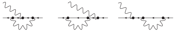
Figure 2: Contributions to the Ward identity in QED. Only the last survives a truncation to one photon and one fermion.

If sector-dependent renormalization is not done, there are uncanceled divergences that arise because the truncation has eliminated contributions that would otherwise cancel against contributions that are kept. The distinction between which are kept and which not is the number of constituents required by intermediate states. This prevents complete removal of the regulators and requires a strategy of seeking a range of regulation parameters (e.g., the PV masses) within which the physical observables are insensitive to the regularization [24]. This minimizes the net effect of two sources of error: the truncation itself, which creates the sensitivity to the regulators, and the presence of PV fields with finite masses.

Sector-dependent bare parameters are chosen to absorb the uncanceled divergences. However, this leads to some unexpected consequences. In QED, there can be coupling renormalization without vacuum polarization; normally the Ward identity prevents this, but a Fock-space truncation violates the Ward identity, as illustrated by Fig. 2. There are also difficulties in removal of regulators, in that Fock-sector probabilities move outside the range of zero to one and some bare couplings can become imaginary. For a consistent theory, the regulators may not be completely removed, just as for the standard approach to renormalization; there may be no uncanceled divergences but Fock-sector probabilities and couplings may take on unphysical values. Any calculation that uses the sector-dependent approach must check for this behavior.

As discussed below, the difficulties are associated with the sector-dependent coupling renormalization. This suggests a middle ground where only bare masses are sector dependent. Such an arrangement can be useful in avoiding the difficulties of sector-dependent renormalization and yet making the invariant mass of higher Fock states more physically reasonable. The scale of the invariant mass for the higher Fock states can be important because Fock states with an invariant mass much larger than the eigenstate mass will not make a significant contribution to the eigenstate. In calculations where the eigenstate/physical mass is much smaller than the bare mass and where higher Fock states should be included, sector-dependent masses will allow a better approximation.

Of course, in the limit that the Fock-space truncation is removed, both the standard renormalization and the sector-dependent renormalization should yield the same result. For the standard case, the limit simply removes the uncanceled divergences. For the sector-dependent case, the bare parameters become sector independent.

For a detailed comparison of the two renormalization methods, consider the dressed-electron state in QED with a truncation to at most one photon [20]. The Fock-state expansion is

$$|\psi^{\pm}(\underline{P})\rangle=\sum_{i}z_{i}b_{i\pm}^{\dagger}(\underline{P})|0\rangle+\sum_{ijs\mu}\int d\underline{k}C_{ijs}^{\mu\pm}(\underline{k})b_{is}^{\dagger}(\underline{P}-\underline{k})a_{j\mu}^{\dagger}(\underline{k})|0\rangle.$$ (168)

A second PV fermion flavor plays no role in this sector, so that sums over the PV fermion indices can be limited to 0 and 1, with $\beta_{1}=1$. The coupled equations for the one-electron amplitude $z_{i}$ and the one-electron/one-photon wave function $C_{ijs}^{\mu\pm}(\underline{k})$ are, with $y=k^{+}/P^{+}$:

$$[M^{2}-m_{i}^{2}]z_{i}=\int(P^{+})^{2}dyd^{2}k_{\perp}\sum_{j,l,\mu}\xi_{l}s_{j}r_{l}\epsilon^{\mu}\left[V_{ji\pm}^{\mu*}(\underline{P}-\underline{k},\underline{P})C^{\mu\pm}_{jl\pm}(\underline{k})+U_{ji\pm}^{\mu*}(\underline{P}-\underline{k},\underline{P})C^{\mu\pm}_{jl\mp}(\underline{k})\right],$$ (169)

and

$$\left[M^{2}-\frac{m_{j}^{2}+k_{\perp}^{2}}{1-y}-\frac{\mu_{l}^{2}+k_{\perp}^{2}}{y}\right]C^{\mu\pm}_{jl\pm}(\underline{k})=\xi_{l}\sum_{i^{\prime}}s_{i^{\prime}}z_{i^{\prime}}P^{+}V_{ji^{\prime}\pm}^{\mu}(\underline{P}-\underline{k},\underline{P}),$$ (170)

$$\left[M^{2}-\frac{m_{j}^{2}+k_{\perp}^{2}}{1-y}-\frac{\mu_{l}^{2}+k_{\perp}^{2}}{y}\right]C^{\mu\pm}_{jl\mp}(\underline{k})=\xi_{l}\sum_{i^{\prime}}s_{i^{\prime}}z_{i^{\prime}}P^{+}U_{ji^{\prime}\pm}^{\mu}(\underline{P}-\underline{k},\underline{P}).$$ (171)

The indexing is arranged such that an index of $i$ or $i^{\prime}$ corresponds to the one-electron sector and $j$ to the one-electron/one-photon sector. For a sector-dependent approach, the mass $m_{i}$ is chosen to be the bare mass $m_{0}$, and $m_{j}$ the physical mass, $M=m_{e}$. In the standard parameterization, all are bare masses.

The coupled equations can be solved analytically [24]. The wave functions $C_{ils}^{\mu\pm}$ are

$$C^{\mu\pm}_{il\pm}(\underline{k})=\xi_{l}\frac{\sum_{j}s_{j}z_{j}P^{+}V_{ij\pm}^{\mu}(\underline{P}-\underline{k},\underline{P})}{M^{2}-\frac{m_{i}^{2}+k_{\perp}^{2}}{1-y}-\frac{\mu_{l}^{2}+k_{\perp}^{2}}{y}},\;\;C^{\mu\pm}_{il\mp}(\underline{k})=\xi_{l}\frac{\sum_{j}s_{j}z_{j}P^{+}U_{ij\pm}^{\mu}(\underline{P}-\underline{k},\underline{P})}{M^{2}-\frac{m_{i}^{2}+k_{\perp}^{2}}{1-y}-\frac{\mu_{l}^{2}+k_{\perp}^{2}}{y}},$$ (172)

and the one-electron amplitudes satisfy

$$(M^{2}-m_{i}^{2})z_{i}=2e_{0}^{2}\sum_{i^{\prime}}s_{i^{\prime}}z_{i^{\prime}}\left[\bar{J}+m_{i}m_{i^{\prime}}\bar{I}_{0}-2(m_{i}+m_{i^{\prime}})\bar{I}_{1}\right],$$ (173)

with

$$\bar{I}_{n}(M^{2}) \equiv \int\frac{dydk_{\perp}^{2}}{16\pi^{2}}\sum_{jl}\frac{s_{j}r_{l}\xi_{l}^{2}}{M^{2}-\frac{m_{j}^{2}+k_{\perp}^{2}}{1-y}-\frac{\mu_{l}^{2}+k_{\perp}^{2}}{y}}\frac{m_{j}^{n}}{y(1-y)^{n}}\,,$$ (174)

$$\bar{J}(M^{2}) \equiv \int\frac{dydk_{\perp}^{2}}{16\pi^{2}}\sum_{jl}\frac{s_{j}r_{l}\xi_{l}^{2}}{M^{2}-\frac{m_{j}^{2}+k_{\perp}^{2}}{1-y}-\frac{\mu_{l}^{2}+k_{\perp}^{2}}{y}}\frac{m_{j}^{2}+k_{\perp}^{2}}{y(1-y)^{2}}.$$ (175)

These integrals satisfy the identity [45] $\bar{J}=M^{2}\bar{I}_{0}$. The coupling coefficient $\xi_{2}$ is fixed by requiring that $M=0$ when $m_{0}=0$, to retain the chiral symmetry [45]. However, to further simplify the calculation, the second PV photon will be dropped and $\xi_{1}=1$ for the first.

The analytic solution for the remaining PV amplitude is

$$z_{1}=\frac{M\pm m_{0}}{M\pm m_{1}}z_{0},$$ (176)

with the bare coupling $\alpha_{0}=e_{0}^{2}/4\pi$ restricted to two possibilities

$$\alpha_{0\pm}=\frac{(M\pm m_{0})(M\pm m_{1})}{8\pi(m_{1}-m_{0})(2\bar{I}_{1}\pm M\bar{I}_{0})}.$$ (177)

The lower sign corresponds to the physical answer, because $m_{0}$ then becomes the physical mass $M=m_{e}$ at zero coupling. The amplitude $z_{0}$ is determined by the normalization.

In this truncation, the limit $m_{1}\rightarrow\infty$ can be taken, to simplify the remaining calculation, leaving only $\mu_{1}$ as the regulating mass. In this limit, $z_{1}$ is zero, $m_{1}z_{1}\rightarrow\pm(M-m_{0})z_{0}$, and

$$\alpha_{0\pm}=\pm\frac{M(M\pm m_{0})}{8\pi(2\bar{I}_{1}\pm M\bar{I}_{0})}.$$ (178)

In the sector-dependent approach, $\bar{I}_{1}$ and $\bar{I}_{0}$ are independent of $m_{0}$. This allows the solution for $\alpha_{0}$ to be rearranged as an explicit expression for $m_{0}$

$$m_{0}=\mp M+8\pi\frac{\alpha_{0\pm}}{M}(2\bar{I}_{1}\pm M\bar{I}_{0}).$$ (179)

The anomalous magnetic moment can be computed in this one-photon truncation as

$$a_{e} = m_{e}\sum_{s\mu}\int d\underline{k}\epsilon^{\mu}\sum_{j=0,2}\xi_{j}^{2}\left(\sum_{i^{\prime}=0}^{1}\sum_{k^{\prime}=j/2}^{j/2+1}\frac{s_{i^{\prime}}r_{k^{\prime}}}{\xi_{k^{\prime}}}C_{i^{\prime}k^{\prime}s}^{\mu+}(\underline{k})\right)^{*}$$

$$\times y\left(\frac{\partial}{\partial k_{x}}+i\frac{\partial}{\partial k_{y}}\right)\left(\sum_{i=0}^{1}\sum_{k=j/2}^{j/2+1}\frac{s_{i}r_{k}}{\xi_{k}}C_{iks}^{\mu-}(\underline{k})\right).$$

In the limit where the PV electron mass $m_{1}$ is infinite, this reduces to

$$a_{e}=\frac{\alpha_{0}}{\pi}m_{e}^{2}z_{0}^{2}\int y^{2}(1-y)dydk_{\perp}^{2}\left(\sum_{k=0}^{1}\frac{r_{k}}{ym_{0}^{2}+(1-y)\mu_{k}^{2}+k_{\perp}^{2}-m_{e}^{2}y(1-y)}\right)^{2}.$$ (181)

For the sector-dependent parameterization, the product $\alpha_{0}z_{0}^{2}$ is equal to the physical coupling $\alpha$, and the bare mass $m_{0}$ in the denominator is replaced by the physical mass $m_{e}$.

Even though we do not include the vacuum polarization contribution to the dressed-electron state, the sector-dependent bare coupling is not equal to the physical coupling. Instead, they are related by $e_{0}=e/z_{0}$, where $z_{0}$ is the amplitude for the bare-electron Fock state computed without projection onto the physical subspace.

In general, the bare coupling is given by $e_{0}=Z_{1}e/\sqrt{Z_{2i}Z_{2f}}Z_{3}$. Here, however, there is no vacuum polarization and $Z_{3}=1$. Also, there is no vertex correction and $Z_{1}=1$. This leaves the wave-function renormalization, which has been split [116] between initial and final contributions $\sqrt{Z_{2i}}$ and $\sqrt{Z_{2f}}$; the split is due to the effects of truncation which limit the contributions to $Z_{2}$ differently on opposite sides of the photon interaction. Figure 2 shows how this works. In the one-photon truncation, only the self-energy loop on one fermion leg can contribute to $Z_{2}$; the loop on the other leg is eliminated by the truncation. This leaves $\sqrt{Z_{2i}Z_{2f}}=z_{0}$ and $\alpha=\alpha_{0}/z_{0}$.

The normalization $\langle\psi^{\sigma^{\prime}}(\underline{P}^{\prime})|\psi^{\sigma}(\underline{P})\rangle=\delta(\underline{P}^{\prime}-\underline{P})\delta_{\sigma^{\prime}\sigma}$ is what determines the amplitude $z_{0}$. In the sector-dependent approach, this reduces to $1=z_{0}^{2}+e_{0}^{2}z_{0}^{2}\tilde{J}_{2}$, with

$$\tilde{J}_{2}\equiv\frac{1}{8\pi^{2}}\int y\,dydk_{\perp}^{2}\sum_{k=0}^{1}r_{k}\frac{(y^{2}+2y-2)m_{e}^{2}+k_{\perp}^{2}}{[k_{\perp}^{2}+(1-y)\mu_{k}^{2}+y^{2}m_{e}^{2}]^{2}}.$$ (182)

With the replacement of $e_{0}$ by $e/z_{0}$, $z_{0}$ can be obtained as $z_{0}=\sqrt{1-e^{2}\tilde{J}_{2}}$, which implies $e_{0}=e/\sqrt{1-e^{2}\tilde{J}_{2}}$. For large $\mu_{1}$, the integral $\tilde{J}_{2}$ behaves as $\tilde{J}_{2}\simeq\frac{1}{8\pi^{2}}\left(\ln\frac{\mu_{1}\mu_{0}^{2}}{m_{e}^{3}}+\frac{9}{8}\right)$. Thus, $e_{0}$ can become imaginary and Fock-sector probabilities, which are proportional to $|z_{0}|^{2}$, can range outside $[0,1]$ as $\mu_{1}\rightarrow\infty$ and $\mu_{0}\rightarrow 0$. Therefore, consistency imposes limits on the UV regulator $\mu_{1}$ and on the infrared regulator $\mu_{0}$.

In the standard parameterization, the bare amplitude is determined by $1=z_{0}^{2}+e^{2}z_{0}^{2}J_{2}$, with

$$J_{2} = \frac{1}{8\pi^{2}}\int y\,dydk_{\perp}^{2}[m_{0}^{2}-4m_{0}m_{e}(1-y)+m_{e}^{2}(1-y)^{2}+k_{\perp}^{2}]$$

$$\times\left(\sum_{k=0}^{1}r_{k}\frac{1}{[k_{\perp}^{2}+(1-y)\mu_{k}^{2}+ym_{0}^{2}-y(1-y)m_{e}^{2}]}\right)^{2}.$$

Thus the bare amplitude is $z_{0}=1/\sqrt{1+e^{2}J_{2}}$, and is driven to zero as $\mu_{1}\rightarrow\infty$. This causes most expectation values also to go to zero. Therefore, in this case there is a limit on $\mu_{1}$, but $\mu_{0}$ can be zero.

The anomalous moment in the sector-dependent case is

$$a_{e}=\frac{\alpha}{\pi}m_{e}^{2}\int y^{2}(1-y)dydk_{\perp}^{2}\sum_{k=0}^{1}r_{k}\left(\frac{1}{ym_{e}^{2}+(1-y)\mu_{k}^{2}+k_{\perp}^{2}-m_{e}^{2}y(1-y)}\right)^{2}$$ (184)

In the $\mu_{1}\rightarrow\infty$, $\mu_{0}\rightarrow 0$ limit, this becomes exactly the Schwinger result [117]

$$a_{e}=\frac{\alpha}{\pi}m_{e}^{2}\int\frac{dydq_{\perp}^{2}/(1-y)}{\left[\frac{m_{e}^{2}+q_{\perp}^{2}}{1-y}+\frac{q_{\perp}^{2}}{y}-m_{e}^{2}\right]^{2}}=\frac{\alpha}{2\pi}.$$ (185)

However, this limit cannot be taken without making the underlying theory inconsistent, and the result for finite regulator masses is quite different from the exact one-photon result, as can be seen in Fig. 3.

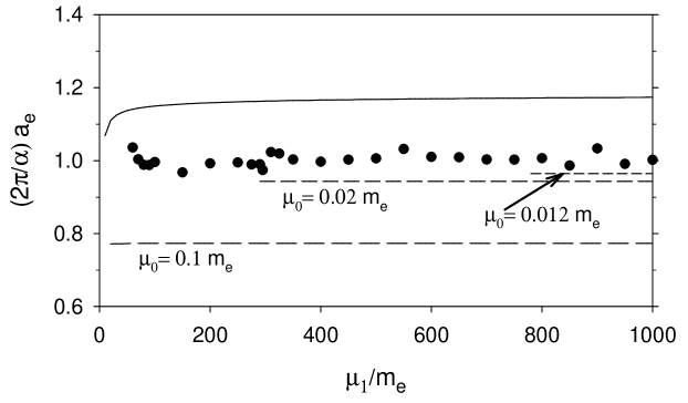
Figure 3: The anomalous moment of the electron in units of the Schwinger term ($\alpha/2\pi$) [117] plotted versus the PV photon mass, $\mu_{1}$, as shown in [20]. The solid line is the standard-parameterization result for the one-electron/one-photon truncation and the dashed lines are the results for sector-dependent parameterization at three different values of photon mass $\mu_{0}$; both use $m_{1}=\infty$. The results for the sector-dependent parameterization are plotted only for values of $\mu_{1}$ for which the probability of the two-particle sector remains between 0 and 1; for values of $\mu_{0}\leq 0.01m_{e}$, this requires $\mu_{1}>1000m_{e}$, which is beyond the range of the plot. For the case of the standard parameterization, $\mu_{0}$ has its physical value of zero. The filled circles are from a calculation with the standard parameterization that includes the self-energy contribution from the one-electron/two-photon sector [20]. It also includes a second PV photon flavor, with its mass, $\mu_{2}$, set to $\sqrt{2}\mu_{1}$; the PV electron mass $m_{1}$ is equal to $2\cdot 10^{4}\,m_{e}$. The variation is due to errors in numerical quadratures.

For both the standard and the sector-dependent parameterizations, truncation of the Fock space results in uncanceled divergences. For the standard case, these divergences are explicit; for the sector-dependent case, they are found in the renormalization of the coupling. However, the sector-dependent coupling renormalization is not the usual coupling renormalization; instead of being driven by vacuum polarization, it is the result of unbalanced wave-function renormalization and the breaking of the Ward identity by the truncation. In both parameterizations, consistency requires a limit on one or more of the regulators, and not all PV masses can be taken to infinity. Any results need to be extracted at finite PV masses. For the sector-dependent approach, this is complicated by infrared divergences.

With so much difficulty caused by the Fock-space truncation, there is a strong motivation to avoid the truncation all together. Unfortunately, a finite calculation in Fock space requires a truncation of some kind. However, this need not be a truncation in particle number. Other truncations are possible, as discussed in the next section.

3.7 Light-Front Coupled-Cluster Method

The LFCC method [21] avoids the difficulties associated with an explicit Fock-space truncation by truncating the set of coupled equations in a very different way. Instead of truncating the number of particles, it truncates the way in which wave functions are related to each other; the wave functions of higher Fock states are determined by the lower-state wave functions and the exponentiation of an operator $T$. Specifically, the eigenstate is written in the form $\sqrt{Z}e^{T}|\phi\rangle$, where $\sqrt{Z}$ is a normalization factor and $|\phi\rangle$ is a state with the minimal number of constituents. The operator $T$ increases particle number and conserves all relevant quantum numbers, including the total light-front momentum. This is in principle exact but also still infinite, because $T$ can have an infinite number of terms.

The truncation made is a truncation of $T$. The original eigenvalue problem becomes a finite-sized eigenvalue problem for the valence state $|\phi\rangle$, combined with auxiliary equations for the terms retained in $T$:

$$P_{v}\overline{{\cal P}^{-}}|\phi\rangle=\frac{M^{2}+P_{\perp}^{2}}{P^{+}}|\phi\rangle,\;\;\;\;(1-P_{v})\overline{{\cal P}^{-}}|\phi\rangle=0.$$ (186)

Here $P_{v}$ is a projection onto the valence sector, and $\overline{{\cal P}^{-}}\equiv e^{-T}{\cal P}^{-}e^{T}$ is the LFCC effective Hamiltonian. The projection $1-P_{v}$ is truncated to provide just enough auxiliary equations to determine the functions in the truncated $T$ operator. The effective Hamiltonian is computed from its Baker–Hausdorff expansion $\overline{{\cal P}^{-}}={\cal P}^{-}+[{\cal P}^{-},T]+\frac{1}{2}[[{\cal P}^{-},T],T]+\cdots$, which can be terminated at the point where more particles are being created than are kept by the truncated projection $1-P_{v}$. The use of the exponential of $T$ rather than some other function is convenient, not only because of the Baker–Hausdorff expansion but more generally because it is invertible; in principle, other functions could be used and would also provide an exact representation until a truncation is made.

The truncation of $T$ can be handled systematically. Terms can be classified by the number of annihilated constituents and the net increase in particle number. For example, in QCD the lowest-order contributions annihilate one particle and increase the total by one. These are one-gluon emission from a quark, quark pair creation from one gluon, and gluon pair creation from one gluon. Each involves a function of relative momentum for the transition from one to two particles. Higher order terms annihilate more particles and/or increase the total by more than one. These provide additional contributions to higher-order wave functions and even to low-order wave functions for more complicated valence states. For example, the wave function for the $|q\bar{q}g\rangle$ Fock state of a meson can have a contribution from a term in $T$ that annihilates a $q\bar{q}$ pair and creates a pair plus a gluon, when this acts on the meson valence state $|q\bar{q}\rangle$.

Zero modes can be included in the LFCC method [118]. The vacuum must then also be computed as a nontrivial eigenstate, which takes the form of a generalized coherent state of zero modes [64, 119]. The zero modes are included by first introducing modes of infinitesimal longitudinal momentum and taking the limit of zero momentum at the end of the calculation. Inclusion of four zero modes in the $T$ operator should be sufficient for a calculation of the critical coupling for dynamical symmetry breaking directly in terms of the vacuum state.

The mathematics of the LFCC method has its origin in the many-body coupled-cluster method [120] used in nonrelativistic nuclear physics and quantum chemistry [121]. The physics is, however, quite different. The many-body method works with a state of a large number of particles and uses the exponentiation of $T$ to build in correlations of excitations to higher single-particle states; the particle number does not change. The LFCC method starts from a small number of constituents in a valence state and uses $e^{T}$ to build states with more particles; the method of solution of the valence-state eigenvalue problem is left unspecified.

The computation of physical observables from matrix elements of operators requires some care. Direct computation would require an infinite sum over Fock space. We instead borrow from the many-body coupled cluster method [121] a construction that computes expectation values from right and left eigenstates of $\overline{{\cal P}^{-}}$. This can be extended to include off-diagonal matrix elements and gauge projections [123].

Consider the expectation value for an operator $\hat{O}$:

$$\langle\hat{O}\rangle=\frac{\langle\phi|e^{T^{\dagger}}\hat{O}e^{T}|\phi\rangle}{\langle\phi|e^{T^{\dagger}}e^{T}|\phi\rangle}.$$ (187)

Define $\overline{O}=e^{-T}\hat{O}e^{T}$ and $\langle\widetilde{\psi}|=\langle\phi|\frac{e^{T^{\dagger}}e^{T}}{\langle\phi|e^{T^{\dagger}}e^{T}|\phi\rangle}$. The expectation value can then be expressed as $\langle\hat{O}\rangle=\langle\widetilde{\psi}|\overline{O}|\phi\rangle$, and the dual vector $\langle\widetilde{\psi}|$ is normalized as

$$\langle\widetilde{\psi}^{\prime}|\phi\rangle=\langle\phi^{\prime}|\frac{e^{T^{\dagger}}e^{T}}{\langle\phi|e^{T^{\dagger}}e^{T}|\phi\rangle}|\phi\rangle=\delta(\underline{P}^{\prime}-\underline{P}).$$ (188)

The effective operator $\overline{O}$ can be computed from its Baker–Hausdorff expansion, $\overline{O}=\hat{O}+[\hat{O},T]+\frac{1}{2}[[\hat{O},T],T]+\cdots$. The dual vector $\langle\widetilde{\psi}|$ is a left eigenvector of $\overline{{\cal P}^{-}}$, as can be seen from

$$\langle\widetilde{\psi}|\overline{{\cal P}^{-}}=\langle\phi|\frac{e^{T^{\dagger}}{\cal P}^{-}e^{T}}{\langle\phi|e^{T^{\dagger}}e^{T}|\phi\rangle}=\langle\phi|\overline{{\cal P}^{-}}^{\dagger}\frac{e^{T^{\dagger}}e^{T}}{\langle\phi|e^{T^{\dagger}}e^{T}|\phi\rangle}=\frac{M^{2}+P_{\perp}^{2}}{P^{+}}\langle\widetilde{\psi}|.$$ (189)

Physical quantities can then be computed from the right and left LFCC eigenstates.

The LFCC method can also be extended to consider time-dependent problems, such as the strong-field dynamics studied by Zhao et al. [106]. The fundamental time-evolution equation ${\cal P}^{-}|\psi\rangle=i\frac{\partial}{\partial x^{+}}|\psi\rangle$ is replaced by

$$P_{v}\left(\overline{{\cal P}^{-}}-i\frac{\partial T}{\partial x^{+}}\right)|\phi\rangle=i\frac{\partial}{\partial x^{+}}|\phi\rangle\;\;\mbox{and}\;\;(1-P_{v})\left(\overline{{\cal P}^{-}}-i\frac{\partial T}{\partial x^{+}}\right)|\phi\rangle=0.$$ (190)

Because $\partial T/\partial x^{+}$ increases particle number, the valence time-evolution equation reduces to

$$P_{v}\overline{{\cal P}^{-}}|\phi\rangle=i\frac{\partial}{\partial x^{+}}|\phi\rangle.$$ (191)

For a single-particle valence state, there is only a time-dependent phase. The time evolution of the $T$ operator is determined by the auxiliary equation, subject to appropriate initial conditions.

3.8 Effective Particles

The renormalization-group procedure for effective particles (RGPEP) [29] has been developed as an extension of the program for nonperturbative QCD by Wilson et al. [31]. It builds on the idea of the similarity renormalization procedure proposed by Glazek and Wilson [32]. Effective Hamiltonians are constructed in terms of creation and annihilation operators for effective particles, which allows for constituent masses that differ from the current masses in the original Hamiltonian. This facilitates a direct connection with constituent quark models and admits a perturbative construction of the effective Hamiltonian.

A given quantum field $\psi_{0}$, built from creation and annihilation operators for bare quanta, is transformed to a field $\psi_{s}={\cal U}_{s}\psi_{0}{\cal U}_{s}^{\dagger}$, built from creation and annihilation operators for effective particles with scale $s$. Kinematical quantum numbers are unchanged; however, masses are treated as dynamical, so that effective particles, such as gluons, can acquire mass. The effective fields are used to construct an effective Hamiltonian ${\cal H}_{t}$, with $t=s^{4}$ a convenient re-parameterization. The effective Hamiltonian is band diagonal, with bandwidth $\sim 1/s$.

For a generic Hamiltonian, written in terms of annihilation operators $q_{0i}$

$${\cal H}_{t}(q_{0i})=\sum_{n=2}^{\infty}\sum_{i_{1},i_{2},\ldots,i_{n}}c_{t}(i_{1},\ldots,i_{n})q_{0i_{1}}^{\dagger}\cdots q_{0i_{n}},$$ (192)

the evolution in the scale $t$ is given by

$$\frac{\partial}{\partial t}{\cal H}_{t}=[[{\cal H}_{f},{\cal H}_{Pt}],{\cal H}_{t}],$$ (193)

where ${\cal H}_{f}\equiv\sum_{i}p_{i}^{-}q_{0i}^{\dagger}q_{0i}$ is the free part of the Hamiltonian and

$${\cal H}_{Pt}\equiv\sum_{n=2}^{\infty}\sum_{i_{1},i_{2},\ldots,i_{n}}\left(\frac{1}{2}\sum_{k=1}^{n}p_{i_{k}}^{-}\right)^{2}c_{t}(i_{1},\ldots,i_{n})q_{0i_{1}}^{\dagger}\cdots q_{0i_{n}}.$$ (194)

This reduces to coupled equations for the coefficients $c_{t}$, which then determine the effective Hamiltonian ${\cal H}_{t}(q_{ti})$ as a polynomial in the effective-particle operators $q_{ti}$.

The band-diagonal structure occurs because the evolution of matrix elements for the interaction Hamiltonian ${\cal H}_{I}\equiv{\cal H}-{\cal H}_{f}$ is given by [29]

$$\frac{\partial}{\partial t}\left(\sum_{mn}|{\cal H}_{Imn}|^{2}\right)=-2\sum_{km}({\cal M}_{km}^{2}-{\cal M}_{mk}^{2})^{2}|{\cal H}_{Ikm}|^{2}\leq 0,$$ (195)

with ${\cal M}_{km}^{2}$ the invariant mass squared for the particles in the $k$th Fock state that are connected by the interaction to the particles in the $m$th state. These Fock states are eigenstates of ${\cal H}_{f}$. Thus, the off-diagonal matrix elements decrease in magnitude with increasing $t=s^{4}$ and do so most rapidly for those states most greatly separated in invariant mass.

Illustrations of the RGPEP in terms of simple theories, where the interaction is a mixing of particle states, can be found in [29]. The solutions are consistent with those obtained with ordinary light-front Fock-space methods.

4 Applications

To illustrate the use of light-front methods, some applications to a range of quantum field theories are considered.

4.1 Quenched Scalar Yukawa Theory

Also known as the (massive) Wick–Cutkosky model [124], quenched scalar Yukawa theory involves charged and neutral scalars coupled by a cubic interaction and quenched, to exclude pair production. The Wick–Cutkosky model focuses on two charged scalars interacting through the exchange of the neutral, which may or may not be massive. Various light-front analyses have been done [125, 126, 127, 73, 128, 129, 130, 131, 132, 18, 133], including both two-dimensional and four-dimensional theories. The most recent work focuses on the construction of the eigenstate for a charged scalar dressed by a cloud of neutrals [134].

Without quenching, the theory is ill defined, having a spectrum that extends to negative infinity, as is generally true of cubic scalar theories [135, 136]. Within a DLCQ approximation, this instability can be difficult to detect [128] unless constrained longitudinal zero modes are included [75]. However, the constraint equation for the neutral scalar can be solved exactly, and the effective interactions that this generates include zero-mode exchange as well as a destabilizing doorway to infinite numbers of charged pairs. The exchange of zero modes is important for obtaining the nominal $1/K^{2}$ convergence of the trapezoidal quadrature rule [73].

The Lagrangian of the model is

$${\cal L}=\partial_{\mu}\chi^{*}\partial^{\mu}\chi-m^{2}|\chi|^{2}+\frac{1}{2}(\partial_{\mu}\phi)^{2}-\frac{1}{2}\mu^{2}\phi^{2}-g\phi|\chi|^{2}.$$ (196)

The Hamiltonian density is

$${\cal H}=|\vec{\partial}_{\perp}\chi|^{2}+m^{2}|\chi|^{2}+\frac{1}{2}(\vec{\partial}_{\perp}\phi)^{2}+\frac{1}{2}\mu^{2}\phi^{2}+g\phi|\chi|^{2}.$$ (197)

The mode expansions for the fields are, as in Sec. 2.2.1,

$$\phi(x)=\int\frac{dp^{+}d^{2}p_{\perp}}{\sqrt{16\pi^{3}p^{+}}}\left[a(\underline{p})e^{-ip\cdot x}+a^{\dagger}(\underline{p})e^{ip\cdot x}\right]$$ (198)

and

$$\chi(x)=\int\frac{dp^{+}d^{2}p_{\perp}}{\sqrt{16\pi^{3}p^{+}}}\left[c_{+}(\underline{p})e^{-ip\cdot x}+c_{-}^{\dagger}(\underline{p})e^{ip\cdot x}\right].$$ (199)

The necessary commutators are given in (10) and (15).

If the $\phi$ zero mode is to be included in a DLCQ calculation, then the mode expansion is periodic on the interval $-L<x^{-}<L$ and $\phi$ is equal to this expansion plus the zero-mode contribution $\phi_{0}(\vec{x}_{\perp})$. When the Euler–Lagrange equation $\partial_{-}\partial_{+}\phi-\vec{\partial}_{\perp}\cdot\vec{\partial}_{\perp}\phi+m^{2}\phi+g|\chi|^{2}=0$ is averaged over the $x^{-}$ interval, only the $\phi_{0}$ contribution survives, leaving the constraint

$$m^{2}\phi_{0}-\nabla_{\perp}^{2}\phi_{0}=-\frac{g}{L}\int_{-L}^{L}dx^{-}|\chi|^{2}.$$ (200)

When $\phi_{0}$ is eliminated from the Hamiltonian density, the $|\chi|^{2}$ term induces a negative term in the Hamiltonian, proportional to $g^{2}|\chi|^{4}$. The expectation value of this term can be made arbitrarily negative by including a large number of charged pairs with momentum fraction $1/K$ [75], and the spectrum must therefore be unbounded from below. This term also contributes an effective quartic interaction between charged scalars that can be interpreted as zero-mode exchange [73].

In the continuum, the light-front Hamiltonian is ${\cal P}^{-}={\cal P}^{-}_{0}+{\cal P}^{-}_{\rm int}$, with

$${\cal P}^{-}_{0}=\int d\underline{p}\frac{m^{2}+\vec{p}_{\perp}^{2}}{p^{+}}\left[c_{+}^{\dagger}(\underline{p})c_{+}(\underline{p})+c_{-}^{\dagger}(\underline{p})c_{-}(\underline{p})\right]+\int d\underline{q}\frac{\mu^{2}+\vec{q}_{\perp}^{2}}{q^{+}}a^{\dagger}(\underline{q})a(\underline{q}).$$ (201)

and

$${\cal P}^{-}_{\rm int} = g\int\frac{d\underline{p}d\underline{q}}{\sqrt{16\pi^{3}p^{+}q^{+}(p^{+}+q^{+})}}\left[\left(c_{+}^{\dagger}(\underline{p}+\underline{q})c_{+}(\underline{p})+c_{-}^{\dagger}(\underline{p}+\underline{q})c_{-}(\underline{p})\right)a(\underline{q})\right.$$

$$\rule{144.54pt}{0.0pt}\left.+a^{\dagger}(\underline{q})\left(c_{+}^{\dagger}(\underline{p})c_{+}(\underline{p}+\underline{q})+c_{-}^{\dagger}(\underline{p})c_{-}(\underline{p}+\underline{q})\right)\right]$$

$$+g\int\frac{d\underline{p}_{1}d\underline{p}_{2}}{\sqrt{16\pi^{3}p_{1}^{+}p_{2}^{+}(p_{1}^{+}+p_{2}^{+})}}\left[c_{+}^{\dagger}(\underline{p}_{1})c_{-}^{\dagger}(\underline{p}_{2})a(\underline{p}_{1}+\underline{p}_{2})+a^{\dagger}(\underline{p}_{1}+\underline{p}_{2})c_{+}(\underline{p}_{1})c_{-}(\underline{p}_{2})\right].$$

For the quenched theory, the second term in ${\cal P}^{-}_{\rm int}$ is dropped.

The Fock-state expansion for the eigenstate with charge $\pm 1$ is

$$|\psi_{\pm}(\underline{P})\rangle=\sum_{n=0}^{\infty}(P^{+})^{n/2}\int\left(\prod_{i}^{n}dx_{i}d^{2}k_{i\perp}\right)\theta(1-\sum_{i}^{n}x_{i})\psi_{n}^{\pm}(x_{i};\vec{k_{i}}_{\perp})|x_{i},\vec{k_{i}}_{\perp},\underline{P},n,\pm\rangle,$$ (203)

with the Fock states written as

$$|x_{i},\vec{k_{i}}_{\perp},\underline{P},n,\pm\rangle=\frac{1}{\sqrt{n!}}c_{\pm}^{\dagger}((1-\sum_{i}^{n}x_{i})P^{+},(1-\sum_{i}^{n}x_{i})\vec{P}_{\perp}-\sum_{i}^{n}\vec{k_{i}}_{\perp})\prod_{i}^{n}a^{\dagger}(x_{i}P^{+},\vec{k_{i}}_{\perp}+x_{i}\vec{P}_{\perp})|0\rangle.$$ (204)

Substitution into the eigenvalue problem ${\cal P}^{-}|\psi_{\pm}(\underline{P})\rangle=\frac{M_{\pm}^{2}+P_{\perp}^{2}}{P^{+}}|\psi_{\pm}(\underline{P})\rangle$ yields the coupled system for the wave functions $\psi_{n}$

$$\left(\frac{m^{2}+(\sum_{i}\vec{k_{i}}_{\perp})^{2}}{1-\sum_{i}x_{i}}+\sum_{i}^{n}\frac{\mu^{2}+k_{i\perp}^{2}}{x_{i}}\right)\psi_{n}^{\pm}(x_{i};\vec{k_{i}}_{\perp})$$

$$+\frac{g}{\sqrt{16\pi^{3}n}}\sum_{j}^{n}\frac{\psi_{n-1}^{\pm}(x_{1},\vec{k_{1}}_{\perp};\ldots;x_{j-1},\vec{k}_{j-1\perp};x_{j+1},\vec{k}_{j+1\perp};\ldots;x_{n},\vec{k_{n}}_{\perp})}{\sqrt{x_{j}(1-\sum_{i\neq j}x_{i})(1-\sum_{i}x_{i})}}$$

$$+\frac{g\sqrt{n+1}}{\sqrt{16\pi^{3}}}\int dyd^{2}q_{\perp}\theta(1-\sum_{i}^{n}x_{i}-y)\frac{\psi_{n+1}^{\pm}(x_{1},\vec{k_{1}}_{\perp};\ldots;x_{n},\vec{k_{n}}_{\perp};y,\vec{q}_{\perp})}{\sqrt{y(1-\sum_{i}x_{i}-y)(1-\sum_{i}x_{i})}}=M_{\pm}^{2}\psi_{n}^{\pm}(x_{i},\vec{k_{i}}_{\perp}).$$

This system is then solved for $M_{\pm}$ and the $\psi_{n}^{\pm}$.

Numerical solutions have been obtained by Li et al. [134]. They used PV regularization with one PV neutral scalar and sector-dependent renormalization. Fock-space truncations up to four particles were investigated. Earlier work [131] had included only three particles (one charged and two neutral). The formulation is slightly different, being based on the covariant light-front dynamics scheme [3], but equivalent. Gauss-Legendre quadrature is used for longitudinal, transverse, and azimuthal integrations. Truncations to two, three, and four particles are compared, in order to study convergence as the Fock-space truncation is relaxed; for weak to moderate coupling, convergence is observed, as illustrated in Fig. 4. The solution is also used to compute the form factor of the dressed charged scalar.

(a)	(b)

Figure 4: Fock sector probabilities as a function of coupling strength $\alpha\equiv\frac{g^{2}}{16\pi m^{2}}$ for the (a) one-particle and (b) two-particle sectors of the dressed charged scalar in quenched scalar Yukawa theory, as shown in [134], for a sequence of Fock-space truncations to two, three, and four particles. The regulating PV mass is set at 15 GeV; the bound-state mass is 0.94 GeV; and the neutral scalar’s mass is 0.14 GeV, chosen to mimic a nucleon dressed by pions.

For the LFCC method, this model is probably the most straightforward application, aside from the original exactly soluble case [21]. The charge $\pm 1$ valence state is just $c_{\pm}^{\dagger}(\underline{P})|0\rangle$, and the exact $T$ operator can be written as

$$T=\sum_{n}\int\prod_{i}^{n}d\underline{q}_{i}d\underline{p}\,t_{n}(\underline{q}_{1},\ldots,\underline{q}_{n},\underline{p})\left(\prod_{i}^{n}a^{\dagger}(\underline{q}_{i})\right)c_{\pm}^{\dagger}(\underline{p})c_{\pm}(\underline{p}+\sum_{i}^{n}\underline{q}_{i}).$$ (206)

The action of $e^{T}$ on the valence state then generates all the Fock states of the quenched theory, with a one-to-one correspondence between the functions $t_{n}$ and the Fock-state wave functions $\psi_{n}$; each is a nonlinear combination of the others. Convergence with respect to truncations of the sum over $n$ in $T$ can be studied.

4.2 $\phi^{4}_{2}$ Theory

Two-dimensional $\phi^{4}$ theory has been a focus for nonperturbative light-front methods from almost the beginning [63, 64, 58, 59, 60, 61, 68], at least partly because the theory provides a relatively simple instance of symmetry breaking and the possible importance of zero modes [57, 75]. The phase transition has been studied on the light front [58], and there have been various attempts at the calculation of critical couplings and even critical exponents [71]. Comparison with results from equal-time quantization require some care if phrased in terms of bare parameters; the renormalization of these parameters is different in the different quantizations [137].

The Lagrangian for $\phi^{4}_{2}$ theory is ${\cal L}=\frac{1}{2}(\partial_{\mu}\phi)^{2}-\frac{1}{2}\mu^{2}\phi^{2}-\frac{\lambda}{4!}\phi^{4}$. Some choose to normalize the coupling differently, replacing $\lambda/4!$ with $\lambda/4$ or even simply $\lambda$. The light-front Hamiltonian density is ${\cal H}=\frac{1}{2}\mu^{2}\phi^{2}+\frac{\lambda}{4!}\phi^{4}$. The mode expansion for the field at zero light-front time is, as usual,

$$\phi=\int\frac{dp^{+}}{\sqrt{4\pi p^{+}}}\left\{a(p^{+})e^{-ip^{+}x^{-}/2}+a^{\dagger}(p^{+})e^{ip^{+}x^{-}/2}\right\},$$ (207)

with the nonzero commutator $[a(p^{+}),a^{\dagger}(p^{\prime+})]=\delta(p^{+}-p^{\prime+})$.

The light-front Hamiltonian can be divided into a kinetic piece and three interaction pieces, each with a different number of creation and annihilation operators, ${\cal P}^{-}={\cal P}^{-}_{11}+{\cal P}^{-}_{13}+{\cal P}^{-}_{31}+{\cal P}^{-}_{22}$, where

$${\cal P}^{-}_{11} = \int dp^{+}\frac{\mu^{2}}{p^{+}}a^{\dagger}(p^{+})a(p^{+}),$$ (208)

$${\cal P}^{-}_{13} = \frac{\lambda}{6}\int\frac{dp_{1}^{+}dp_{2}^{+}dp_{3}^{+}}{4\pi\sqrt{p_{1}^{+}p_{2}^{+}p_{3}^{+}(p_{1}^{+}+p_{2}^{+}+p_{3}^{+})}}a^{\dagger}(p_{1}^{+}+p_{2}^{+}+p_{3}^{+})a(p_{1}^{+})a(p_{2}^{+})a(p_{3}^{+}),$$ (209)

$${\cal P}^{-}_{31} = \frac{\lambda}{6}\int\frac{dp_{1}^{+}dp_{2}^{+}dp_{3}^{+}}{4\pi\sqrt{p_{1}^{+}p_{2}^{+}p_{3}^{+}(p_{1}^{+}+p_{2}^{+}+p_{3}^{+})}}a^{\dagger}(p_{1}^{+})a^{\dagger}(p_{2}^{+})a^{\dagger}(p_{3}^{+})a(p_{1}^{+}+p_{2}^{+}+p_{3}^{+}),$$ (210)

$${\cal P}^{-}_{22} = \frac{\lambda}{4}\int\frac{dp_{1}^{+}dp_{2}^{+}}{4\pi\sqrt{p_{1}^{+}p_{2}^{+}}}\int\frac{dp_{1}^{\prime+}dp_{2}^{\prime+}}{\sqrt{p_{1}^{\prime+}p_{2}^{\prime+}}}\delta(p_{1}^{+}+p_{2}^{+}-p_{1}^{\prime+}-p_{2}^{\prime+})a^{\dagger}(p_{1}^{+})a^{\dagger}(p_{2}^{+})a(p_{1}^{\prime+})a(p_{2}^{\prime+}).$$ (211)

The eigenstate with momentum $P^{+}$ is expanded as

$$|\psi(P^{+})\rangle=\sum_{n}(P^{+})^{\frac{n-1}{2}}\int\prod_{i}^{n}dy_{i}\delta(1-\sum_{i}^{n}y_{i})\psi_{n}(y_{i})\frac{1}{\sqrt{n!}}\prod_{i=1}^{n}a^{\dagger}(y_{i}P^{+})|0\rangle,$$ (212)

with the sum over $n$ restricted to odd or even numbers, because ${\cal P}^{-}$ does not mix the two cases. On substitution of this Fock-state expansion and a dimensionless coupling $g=\lambda/4\pi\mu^{2}$, the light-front Hamiltonian eigenvalue problem ${\cal P}^{-}|\psi(P^{+})\rangle=\frac{M^{2}}{P^{+}}|\psi(P^{+})\rangle$ becomes

$$\frac{n}{y_{1}}\psi_{n}(y_{i})+\frac{g}{4}\frac{n(n-1)}{\sqrt{y_{1}y_{2}}}\int\frac{dx_{1}dx_{2}}{\sqrt{x_{1}x_{2}}}\delta(y_{1}+y_{2}-x_{1}-x_{2})\psi_{n}(x_{1},x_{2},y_{3},\ldots,y_{n})$$ (213)

$$+\frac{g}{6}n\sqrt{(n+2)(n+1)}\int\frac{dx_{1}dx_{2}dx_{3}}{\sqrt{y_{1}x_{1}x_{2}x_{3}}}\delta(y_{1}-x_{1}-x_{2}-x_{3})\psi_{n+2}(x_{1},x_{2},x_{3},y_{2},\ldots,y_{n})$$

$$+\frac{g}{6}\frac{(n-2)\sqrt{n(n-1)}}{\sqrt{y_{1}y_{2}y_{3}(y_{1}+y_{2}+y_{3})}}\psi_{n-2}(y_{1}+y_{2}+y_{3},y_{4},\ldots,y_{n})=\frac{M^{2}}{\mu^{2}}\psi_{n}(y_{i}).$$

This coupled system can then be solved for the mass $M$ and wave functions $\psi_{n}$. The fully symmetric polynomials discussed in Sec. 3.4 were designed for just this purpose; some results obtained in this way are discussed below.

The earliest and highest resolution calculations have been done with DLCQ. The resolution has been taken high enough to obtain degeneracy between the odd and even sectors in the broken-symmetry case [59], following the work of Rozowsky and Thorn [57] where degeneracy was indicated but not achieved at their lower resolution. Figure 5 contains two samples of the high-resolution DLCQ results, which show the degeneracy between odd and even states in the infinite-resolution limit. Low-level excitations at strong coupling can be associated with kink-antikink states [60, 61, 138]. These may indicate formation of a kink condensate driving the transition to symmetry restoration for the negative mass-squared case.

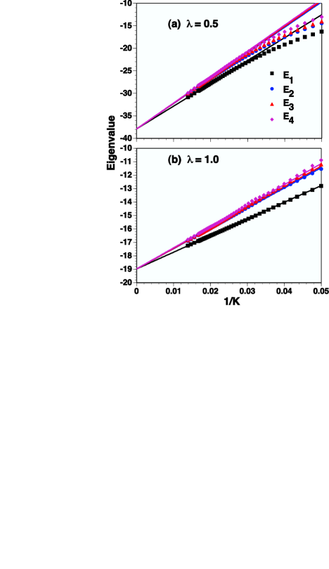
Figure 5: Mass-squared eigenvalues for odd and even states in the broken-symmetry phase, in units of $\mu^{2}$, from DLCQ calculations with resolution $K$, from [59]. The values of the coupling constant $\lambda$ are quoted in units of $\mu^{2}$, where $\mu$ is the bare mass of the constituents. The solid lines are extrapolated fits to the numerical results.

Inclusion of zero modes can improve the DLCQ calculations. The solution of the DLCQ constraint equation for the zero mode can be used to study the critical coupling and critical exponents [71]. The solution can also be used to develop a controlled series of effective interactions that improve the numerical convergence [75].

The LFCC method has also been applied to $\phi^{4}_{2}$ theory [139]. For the odd case, the valence state is the one-particle state $a^{\dagger}(P^{+})|0\rangle$. The leading contribution to the $T$ operator is

$$T_{2}\equiv\int dp_{1}^{+}dp_{2}^{+}dp_{3}^{+}t_{2}(p_{1}^{+},p_{2}^{+},p_{3}^{+})a^{\dagger}(p_{1}^{+})a^{\dagger}(p_{2}^{+})a^{\dagger}(p_{3}^{+})a(p_{1}^{+}+p_{2}^{+}+p_{3}^{+});$$ (214)

the function $t_{2}$ is symmetric in its arguments. For $T$ truncated to $T_{2}$, the projection $1-P_{v}$ is truncated to projection onto the three-particle state $a^{\dagger}(p_{1}^{+})a^{\dagger}(p_{2}^{+})a^{\dagger}(p_{3}^{+})|0\rangle$. Zero modes can also be included [118].

The valence equation, the first in (186), can be reduced to

$$1+g\int\frac{dx_{1}dx_{2}}{\sqrt{x_{1}x_{2}x_{3}}}\tilde{t}_{2}(x_{1},x_{2},x_{3})=M^{2}/\mu^{2},$$ (215)

where $\tilde{t}_{2}$ is a rescaled function of longitudinal momentum fractions $x_{i}=p_{i}^{+}/P^{+}$,

$$\tilde{t}_{2}(x_{1},x_{2},x_{3})\equiv P^{+}t_{2}(x_{1}P^{+},x_{2}P^{+},x_{3}P^{+}).$$ (216)

Given the definition of a dimensionless mass shift

$$\Delta\equiv g\int\frac{dx_{1}dx_{2}}{\sqrt{x_{1}x_{2}x_{3}}}\tilde{t}_{2}(x_{1},x_{2},x_{3}),$$ (217)

the valence equation can be written as simply $M^{2}=(1+\Delta)\mu^{2}$.

The reduced auxiliary equation, from the second equation in (186), is

$$\frac{1}{6}\frac{g}{\sqrt{y_{1}y_{2}y_{3}}}+\frac{M^{2}}{\mu^{2}}\left(\frac{1}{y_{1}}+\frac{1}{y_{2}}+\frac{1}{y_{3}}-1\right)\tilde{t}_{2}(y_{1},y_{2},y_{3})$$

$$+\frac{g}{2}\left[\int_{0}^{1-y_{1}}dx_{1}\frac{\tilde{t}_{2}(y_{1},x_{1},1-y_{1}-x_{1})}{\sqrt{x_{1}y_{2}y_{3}(1-y_{1}-x_{1})}}+(y_{1}\leftrightarrow y_{2})+(y_{1}\leftrightarrow y_{3})\right]$$

$$-\frac{\Delta}{2}\left(\frac{1}{y_{1}}+\frac{1}{y_{2}}+\frac{1}{y_{3}}\right)\tilde{t}_{2}(y_{1},y_{2},y_{3})$$

$$+\frac{3g}{2}\left\{\int_{y_{1}/(1-y_{2})}^{1}d\alpha_{1}\int_{0}^{1-\alpha_{1}}d\alpha_{2}\frac{\tilde{t}_{2}(y_{1}/\alpha_{1},y_{2},1-y_{1}/\alpha_{1}-y_{2})\tilde{t}_{2}(\alpha_{1},\alpha_{2},\alpha_{3})}{\sqrt{\alpha_{1}\alpha_{2}\alpha_{3}y_{3}(\alpha_{1}-y_{1}-\alpha_{1}y_{2})}}\right.$$

$$\rule{158.99377pt}{0.0pt}\left.+(y_{1}\leftrightarrow y_{2})+(y_{1}\leftrightarrow y_{3})\rule{0.0pt}{10.84006pt}\right\}$$

$$+\frac{3g}{2}\left\{\left[\int_{y_{1}+y_{2}}^{1}d\alpha_{1}\int_{0}^{1-\alpha_{1}}d\alpha_{2}\frac{\tilde{t}_{2}(y_{1}/\alpha_{1},y_{2}/\alpha_{1},1-(y_{1}+y_{2})/\alpha_{1})\tilde{t}_{2}(\alpha_{1},\alpha_{2},\alpha_{3})}{\alpha_{1}\sqrt{\alpha_{2}\alpha_{3}y_{3}(\alpha_{1}-y_{1}-y_{2})}}\right.\right.$$

$$\rule{180.67499pt}{0.0pt}\left.+(y_{2}\leftrightarrow y_{3})\rule{0.0pt}{10.84006pt}\right]$$

$$\rule{72.26999pt}{0.0pt}\left.+(y_{1}\leftrightarrow y_{2})+(y_{1}\leftrightarrow y_{3})\rule{0.0pt}{10.84006pt}\right\}=0,$$

with $y_{i}=q_{i}^{+}/P^{+}$. For comparison, consider a Fock-state truncation that produces the same number of equations. The truncated eigenstate then contains only one and three-body contributions and the coupled system of integral equations reduces to

$$1+g\int\frac{dx_{1}dx_{2}}{\sqrt{x_{1}x_{2}x_{3}}}\tilde{\psi}_{3}(x_{1},x_{2},x_{3})=M^{2}/\mu^{2},$$

$$\frac{1}{6}\frac{g}{\sqrt{y_{1}y_{2}y_{3}}}+\left(\frac{1}{y_{1}}+\frac{1}{y_{2}}+\frac{1}{y_{3}}-\frac{M^{2}}{\mu^{2}}\right)\tilde{\psi}_{3}(y_{1},y_{2},y_{3})$$

$$+\frac{g}{2}\left[\int_{0}^{1-y_{1}}dx_{1}\frac{\tilde{\psi}_{3}(x_{1},y_{1},1-y_{1}-x_{1})}{\sqrt{x_{1}(1-y_{1}-x_{1})y_{2}y_{3}}}+(y_{1}\leftrightarrow y_{2})+(y_{1}\leftrightarrow y_{3})\rule{0.0pt}{21.68121pt}\right]=0,$$

with $\tilde{\psi}_{3}\equiv\psi_{3}/(\sqrt{6}\psi_{1})$.

In each case, the first equation is of the same form; it provides for the self-energy correction of the bare mass to yield the physical mass. The second equations, (4.2) and (4.2), however, differ significantly. The LFCC auxiliary equation includes the physical mass in the three-body kinetic energy; the three-body equation of the Fock-truncation approach has only the bare mass and would require sector-dependent renormalization [16, 17, 18, 20] to compensate. The fourth LFCC term is the nonperturbative analog of the wave-function renormalization counterterm. The last two terms are partial resummations of higher-order loops. These terms do not appear in the truncated coupled system because the loops have intermediate states that are removed by the truncation.

These equations are solved numerically in [139], and more recently for higher Fock-space truncation, with basis function expansions that use the fully-symmetric multivariate polynomials [34]. The converged results for the mass-squared eigenvalues are shown in Fig. 6. There is a distinct difference between the LFCC approximation and the lowest-order Fock-space truncation. This arises from two factors: the correct kinetic-energy mass in each sector of the LFCC calculation and contributions from higher Fock states. When the lowest-order Fock-space truncation method is modified with sector-dependent masses [16, 17, 18, 20], the resulting mass values are intermediate between the these two sets. The higher-order Fock-space truncations, at five-body and seven-body Fock sectors, are in agreement to within numerical error, indicating convergence in the Fock-state expansion. The LFCC result is close to these, implying excellent representation of contributions from the higher Fock states.

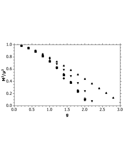
Figure 6: Mass-squared ratios $M^{2}/\mu^{2}$ versus dimensionless coupling strength $g$ for the LFCC approximation (circles), the Fock-space truncation to three (up triangles), five (squares), and seven (diamonds) particles, and the Fock-space truncation to three with sector-dependent masses (down triangles) for the odd eigenstate of $\phi_{1+1}^{4}$. The error bars reflect uncertainties in the numerical extrapolations. For small $g$, all of the results overlap; for all $g$, the results for the five and seven-particle truncations are nearly indistinguishable, indicating convergence of the Fock-state expansion.

The Fock-space-converged results also allow estimation of the critical coupling of the theory. In the plot, the mass gap vanishes at $g\simeq 2.1$. This is consistent with a much older light-front (DLCQ) calculation by Harindranath and Vary [63] but not with equal-time calculations, as reported by Rychkov and Vitale [140]. In their units, the LFCC result for the critical coupling is $1.1$, and the DLCQ result is 1.38, to compare with their result of 2.97. However, these are values of the ratio of bare parameters of the Lagrangian; as such, the different quantizations need not yield the same values. In fact, earlier work by Burkardt [137] has shown that, while the bare coupling $\lambda$ is unchanged, the renormalization of the bare mass $\mu$ is different in the two quantizations by a computable amount. The bare mass is renormalized by tadpole contributions in equal-time quantization but not in light-front quantization, and the two different masses are related by [137]

$$\mu_{\rm LF}^{2}=\mu_{\rm ET}^{2}+\lambda\left[\langle 0|:\frac{\phi^{2}}{2}:|0\rangle-\langle 0|:\frac{\phi^{2}}{2}:|0\rangle_{\rm free}\right].$$ (221)

The vacuum expectation values of $\phi^{2}$ resum the tadpole contributions; the subscript free indicates the vev with $\lambda=0$. This distinction between bare masses in the two quantizations implies that the dimensionless coupling $g=\lambda/4\pi\mu^{2}$ is also not the same. Estimates of the critical coupling must then be adjusted for the difference if they are to be compared.

4.3 Yukawa Theory

The standard Yukawa theory of fermions interacting with scalars has received considerable attention. A series of papers [94, 109, 81] investigated the dressed fermion state on the light front, using PV regularization, DLCQ, and Gauss–Legendre quadrature. These built on preliminary work with a soluble model [78, 141] and considered various truncations as well as different choices for the PV sector. A number of properties of the dressed-fermion eigenstate were extracted from the Fock-state wave functions, including average numbers of constituents and their average momenta, structure functions, and the average radius.

An analysis of the exactly soluble case of PV-mass degeneracy was also done [142], in order to better understand the connection with equal-time quantization, through the exact operator solution of the theory, and to consider the possibility of developing a perturbation theory based on mass differences; the eigenvalue problem in the Fock basis is exactly soluble because it is triangular when the PV masses are degenerate with the physical masses.

The one-loop fermion self-energy in light-front Yukawa theory requires three PV scalars to subtract the quadratic and log divergences and to restore chiral symmetry in the massless limit [143]. In the preliminary work [78], a DLCQ approximation of this self-energy was shown to require a discrete set of PV Fock states that was only 1.5 times the size of the set of ordinary Fock states; this provided encouragement that the computational load associated with the introduction of the additional PV states was not too large.

The first calculation [94], with the DLCQ approach, used these three scalars. Subsequent work [109, 81] used one PV scalar and one PV fermion, coupled in null combinations. The advantage of the newer PV scheme was in the absence of four-point instantaneous fermion interactions, which are independent of the fermion mass and cancel between physical and PV fermions. Their absence significantly simplifies the matrix representation of the Hamiltonian, which then contains only three-point vertices. This later work truncated the Fock space to include no more than two bosons dressing the fermion and excluded pair production. The one-boson truncation [109] is exactly solvable; the two-boson truncation [81] requires numerical methods.

Closely following this work, there was a sequence of investigations [144, 145, 146, 19, 147] within the context of covariant light-front dynamics and eventually employing PV regularization and sector-dependent renormalization. This work included computation of the anomalous magnetic moment [19] and even the electromagnetic form factors [147] of the fermion dressed by one or two bosons. Dependence on the cutoff is eliminated to within numerical accuracy. This is closely related to earlier work by Glazek and Perry [148] on the sector-dependent approach to Yukawa theory; they show that triviality imposes a limit on the cutoff.

The primary gain from this work has been the experience of working with fermions in nonperturbative calculations without the additional complications of QED. For example, the form of PV regularization which eliminates instantaneous fermion interactions was first developed in Yukawa theory before being considered for QED. Yukawa theory also offers the opportunity to study an unquenched theory and the associated renormalizations of the charge and scalar mass, something for which the unstable scalar Yukawa theory cannot be used. This aspect is largely unexplored at present, although some preliminary work has been done [94, 147]. Applications to modeling of scalar meson exchange in nuclear physics are quite limited, given that accurate phenomenology requires a more sophisticated interaction [149].

The Yukawa-theory Lagrangian, regulated by one PV scalar and one PV fermion, is

$${\cal L}=\frac{1}{2}(\partial_{\mu}\phi_{0})^{2}-\frac{1}{2}\mu_{0}^{2}\phi_{0}^{2}-\frac{1}{2}(\partial_{\mu}\phi_{1})^{2}+\frac{1}{2}\mu_{1}^{2}\phi_{1}^{2}$$

$$+\frac{i}{2}\left(\overline{\psi}_{0}\gamma^{\mu}\partial_{\mu}-(\partial_{\mu}\overline{\psi}_{0})\gamma^{\mu}\right)\psi_{0}-m_{0}\overline{\psi}_{0}\psi_{0}$$

$$-\frac{i}{2}\left(\overline{\psi}_{1}\gamma^{\mu}\partial_{\mu}-(\partial_{\mu}\overline{\psi}_{1})\gamma^{\mu}\right)\psi_{1}+m_{1}\overline{\psi}_{1}\psi_{1}-g(\phi_{0}+\phi_{1})(\overline{\psi}_{0}+\overline{\psi}_{1})(\psi_{0}+\psi_{1}).$$

The subscript 0 indicates a physical field and 1, a PV field. The fermion masses are denoted by $m_{i}$, and the boson masses by $\mu_{j}$. When fermion pairs are excluded, the resulting light-front Hamiltonian is

$${\cal P}^{-}=\sum_{i,s}\int d\underline{p}\frac{m_{i}^{2}+p_{\perp}^{2}}{p^{+}}(-1)^{i}b_{i,s}^{\dagger}(\underline{p})b_{i,s}(\underline{p})+\sum_{j}\int d\underline{q}\frac{\mu_{j}^{2}+q_{\perp}^{2}}{q^{+}}(-1)^{j}a_{j}^{\dagger}(\underline{q})a_{j}(\underline{q})$$

$$+\sum_{i,j,k,s}\int d\underline{p}d\underline{q}\left\{\left[V_{-2s}^{*}(\underline{p},\underline{q})+V_{2s}(\underline{p}+\underline{q},\underline{q})\right]b_{j,s}^{\dagger}(\underline{p})a_{k}^{\dagger}(\underline{q})b_{i,-s}(\underline{p}+\underline{q})\right.$$

$$\left.\rule{36.135pt}{0.0pt}+\left[U_{j}(\underline{p},\underline{q})+U_{i}(\underline{p}+\underline{q},\underline{q})\right]b_{j,s}^{\dagger}(\underline{p})a_{k}^{\dagger}(\underline{q})b_{i,s}(\underline{p}+\underline{q})+h.c.\right\},$$

where $a^{\dagger}$ creates a boson and $b^{\dagger}$ a fermion, and

$$U_{j}(\underline{p},\underline{q})\equiv\frac{g}{\sqrt{16\pi^{3}}}\frac{m_{j}}{p^{+}\sqrt{q^{+}}},\;\;V_{2s}(\underline{p},\underline{q})\equiv\frac{g}{\sqrt{8\pi^{3}}}\frac{{\vec{\epsilon}}_{2s}^{\,*}\cdot{\vec{p}}_{\perp}}{p^{+}\sqrt{q^{+}}},\;\;{\vec{\epsilon}}_{2s}\equiv-\frac{1}{\sqrt{2}}(2s,i).$$ (224)

The nonzero (anti)commutators are

$$\left[a_{i}(\underline{q}),a_{j}^{\dagger}(\underline{q}^{\prime})\right]=(-1)^{i}\delta_{ij}\delta(\underline{q}-\underline{q}^{\prime}),\;\;\left\{b_{i,s}(\underline{p}),b_{j,s^{\prime}}^{\dagger}(\underline{p}^{\prime})\right\}=(-1)^{i}\delta_{ij}\delta_{s,s^{\prime}}\delta(\underline{p}-\underline{p}^{\prime}).$$ (225)

The opposite signature of the PV fields is the reason that no instantaneous fermion terms appear in ${\cal P}^{-}$; they are individually independent of the fermion mass and cancel between instantaneous physical and PV fermions.

This scheme was explored in the unphysical equal-mass limit where analytic solutions of the field-theoretic eigenstate can be obtained without explicit truncation [142]. The simplest such solution takes the form

$$\beta_{+,\underline{k}}^{\dagger}|0\rangle+mg\int_{0}^{k^{+}}d\underline{l}{U(\underline{k},\underline{l})\over E_{1,0}(\underline{k})-E_{1,1}(\underline{l},\underline{k}-\underline{l})}b_{+,\underline{l}}^{\dagger}a_{\underline{k}-\underline{l}}^{\dagger}|0\rangle+g\int_{0}^{k^{+}}d\underline{l}{V(\underline{k},\underline{l})\over E_{1,0}(\underline{k})-E_{1,1}(\underline{l},\underline{k}-\underline{l})}b_{-,\underline{l}}^{\dagger}a_{\underline{k}-\underline{l}}^{\dagger}|0\rangle,$$ (226)

where $\beta^{\dagger}$, $b^{\dagger}$, and $a^{\dagger}$ are creation operators for null combinations of the fields, $m\equiv m_{0}=m_{1}$ is the fermion mass, and

$$U(\underline{k},\underline{l})\equiv{1\over\sqrt{16\pi^{3}}}{1\over\sqrt{k^{+}-l^{+}}}\left({1\over l^{+}}+{1\over k^{+}}\right)\,,$$ (227)

$$V(\underline{k},\underline{l})\equiv{1\over\sqrt{16\pi^{3}}}{1\over\sqrt{k^{+}-l^{+}}}\left({-l_{1}-il_{2}\over l^{+}}+{k_{1}+ik_{2}\over k^{+}}\right)\,.$$ (228)

The eigenvalue of the state is $(k_{\perp}^{2}+m^{2})/k^{+}$. Such analytic solutions provide a convenient check for numerical calculations.

The Fock-state expansion for the dressed-fermion state with $J_{z}=+1/2$ is

$$|\psi_{+}(\underline{P})\rangle=\sum_{i}z_{i}b_{i+}^{\dagger}(\underline{P})|0\rangle+\sum_{ijs}\int d\underline{q}f_{ijs}(\underline{q})b_{is}^{\dagger}(\underline{P}-\underline{q})a_{j}^{\dagger}(\underline{q})|0\rangle$$

$$+\sum_{ijks}\int d\underline{q}_{1}d\underline{q}_{2}f_{ijks}(\underline{q}_{1},\underline{q}_{2})\frac{1}{\sqrt{1+\delta_{jk}}}b_{is}^{\dagger}(\underline{P}-\underline{q}_{1}-\underline{q}_{2})a_{j}^{\dagger}(\underline{q}_{1})a_{k}^{\dagger}(\underline{q}_{2})|0\rangle+\ldots,$$

It is normalized by the requirement $\langle\psi_{\sigma^{\prime}}(\underline{P}^{\prime})|\psi_{\sigma}(\underline{P})\rangle=\delta_{\sigma\sigma^{\prime}}\delta(\underline{P}^{\prime}-\underline{P})$. The wave functions $f$ that define this state must satisfy the usual coupled system of equations The first three coupled equations are

$$m_{i}^{2}z_{i} + \sum_{i^{\prime},j}(-1)^{i^{\prime}+j}P^{+}\int^{P^{+}}d\underline{q}\left\{f_{i^{\prime}j-}(\underline{q})[V_{+}(\underline{P}-\underline{q},\underline{q})+V_{-}^{*}(\underline{P},\underline{q})]\right.$$ (230)

$$\left.+f_{i^{\prime}j+}(\underline{q})[U_{i^{\prime}}(\underline{P}-\underline{q},\underline{q})+U_{i}(\underline{P},\underline{q})]\right\}=M^{2}z_{i},$$

$$\left[\frac{m_{i}^{2}+q_{\perp}^{2}}{1-y}+\frac{\mu_{j}^{2}+q_{\perp}^{2}}{y}\right]f_{ijs}(\underline{q})+\sum_{i^{\prime}}(-1)^{i^{\prime}}\left\{z_{i^{\prime}}\delta_{s,-}[V_{+}^{*}(\underline{P}-\underline{q},\underline{q})+V_{-}(\underline{P},\underline{q})]\right.$$

$$\rule{144.54pt}{0.0pt}\left.+z_{i^{\prime}}\delta_{s,+}[U_{i}(\underline{P}-\underline{q},\underline{q})+U_{i^{\prime}}(\underline{P},\underline{q})]\right\}$$

$$+2\sum_{i^{\prime},k}\frac{(-1)^{i^{\prime}+k}}{\sqrt{1+\delta_{jk}}}P^{+}\int^{P^{+}-q^{+}}d\underline{q}^{\prime}\left\{f_{i^{\prime}jk,-s}(\underline{q},\underline{q}^{\prime})[V_{2s}(\underline{P}-\underline{q}-\underline{q}^{\prime},\underline{q}^{\prime})\right.$$

$$\rule{144.54pt}{0.0pt}+V_{-2s}^{*}(\underline{P}-\underline{q},\underline{q}^{\prime})]$$

$$\left.+f_{i^{\prime}jks}(\underline{q},\underline{q}^{\prime})[U_{i^{\prime}}(\underline{P}-\underline{q}-\underline{q}^{\prime},\underline{q}^{\prime})+U_{i}(\underline{P}-\underline{q},\underline{q}^{\prime})]\right\}=M^{2}f_{ijs}(\underline{q}),$$

and

$$\left[\frac{m_{i}^{2}+(\vec{q}_{1\perp}+\vec{q}_{2\perp})^{2}}{1-y_{1}-y_{2}}+\frac{\mu_{j}^{2}+q_{1\perp}^{2}}{y_{1}}+\frac{\mu_{k}^{2}+q_{2\perp}^{2}}{y_{2}}\right]f_{ijks}(\underline{q_{1}},\underline{q_{2}})$$

$$+\sum_{i^{\prime}}(-1)^{i^{\prime}}\frac{\sqrt{1+\delta_{jk}}}{2}P^{+}\left\{f_{i^{\prime}j,-s}(\underline{q_{1}})[V_{-2s}^{*}(\underline{P}-\underline{q_{1}}-\underline{q_{2}},\underline{q_{2}})\right.$$

$$\rule{144.54pt}{0.0pt}+V_{2s}(\underline{P}-\underline{q_{1}},\underline{q_{2}})]$$

$$+f_{i^{\prime}js}(\underline{q_{1}})[U_{i}(\underline{P}-\underline{q_{1}}-\underline{q_{2}},\underline{q_{2}})+U_{i^{\prime}}(\underline{P}-\underline{q_{1}},\underline{q_{2}})]$$

$$+f_{i^{\prime}k,-s}(\underline{q_{2}})[V_{-2s}^{*}(\underline{P}-\underline{q_{1}}-\underline{q_{2}},\underline{q_{1}})+V_{2s}(\underline{P}-\underline{q_{2}},\underline{q_{1}})]$$

$$\left.+f_{i^{\prime}ks}(\underline{q_{2}})[U_{i}(\underline{P}-\underline{q_{1}}-\underline{q_{2}},\underline{q_{1}})+U_{i^{\prime}}(\underline{P}-\underline{q_{2}},\underline{q_{1}})]\right\}+\ldots$$

$$=M^{2}f_{ijks}(\underline{q_{1}},\underline{q_{2}}).$$

To best interpret the norms of different Fock sectors, the physical wave functions were defined as the coefficients of Fock states containing only positive-norm particles. This reduction can be achieved by requiring all Fock states to be expressed in terms of the positive-norm creation operators $b_{0s}^{\dagger}$ and $a_{0}^{\dagger}$ and the zero-norm combinations $b_{s}^{\dagger}\equiv b_{0s}^{\dagger}+b_{1s}^{\dagger}$ and $a^{\dagger}\equiv a_{0}^{\dagger}+a_{1}^{\dagger}$. Any term containing a $b_{s}^{\dagger}$ or an $a^{\dagger}$, which would be annihilated by the PV-generalized electromagnetic current, is discarded, leaving the physical state

$$|\psi_{+}\rangle_{\rm phys}=(z_{0}-z_{1})b_{1+}^{\dagger}(\underline{P})|0\rangle+\sum_{s}\int d\underline{q}\left(\sum_{ij}(-1)^{i+j}f_{ijs}(\underline{q})\right)b_{0s}^{\dagger}(\underline{P}-\underline{q})a_{0}^{\dagger}(\underline{q})|0\rangle$$

$$+\sum_{s}\int d\underline{q}_{1}d\underline{q}_{2}\left(\sum_{ijk}(-1)^{i+j+k}f_{ijks}(\underline{q}_{1},\underline{q}_{2})\frac{1}{\sqrt{1+\delta_{jk}}}\right)$$

$$\rule{144.54pt}{0.0pt}\times b_{0s}^{\dagger}(\underline{P}-\underline{q}_{1}-\underline{q}_{2})a_{0}^{\dagger}(\underline{q}_{1})a_{0}^{\dagger}(\underline{q}_{2})|0\rangle+\ldots,$$

From this state various physical quantities are extracted, including the boson structure function for constituent-fermion helicity $s$

$$f_{Bs}(y)=\int d\underline{q}\delta(y-q^{+}/P^{+})\left|\sum_{ij}(-1)^{i+j}f_{ijs}(\underline{q})\right|^{2}$$

$$+\int\prod_{n=1}^{2}d\underline{q_{n}}\sum_{n=1}^{2}\delta(y-q_{n}^{+}/P^{+})\left|\sum_{ijk}(-1)^{i+j+k}f_{ijks}(\underline{q_{n}})\right|^{2}+\ldots$$

In traditional DLCQ, the lower bound of $1/K$ on longitudinal momentum fractions provides a natural cutoff in the number of equations. The range of the transverse integrations is cut off by imposing $p_{i\perp}^{2}/x_{i}<\Lambda^{2}$ for each particle in a Fock state; this reduces the DLCQ matrix problem to a finite size. The transverse momentum indices $n_{x}$ and $n_{y}$ are limited by a transverse resolution $N$. For a reduced set of equations, alternative quadratures are more efficient. In particular, the transverse momentum $q_{\perp}$ can be mapped to a finite range that compresses the wave function’s tail to a relatively small region, so that a Gauss–Legendre quadrature can yield a good approximation [81].

Given such a discretization and the consequent finite matrix eigenvalue problem, one can compute mass eigenvalues and associated wave functions. The bare parameters $g$ and $m_{0}$ can be fixed by fitting “physical” constraints, such as specifying the dressed-fermion mass $M$ and its radius. In principle, one then takes the infinite resolution and infinite momentum volume limits, as well as the infinite PV-mass limits.

4.4 Supersymmetric Yang–Mills theory

A number of applications of SDLCQ to supersymmetric Yang–Mills (SYM) theories have been carried out by the SDLCQ collaboration [33, 150, 86, 87, 151, 83, 152, 153, 154, 155, 156, 157, 158, 159, 160, 161, 162]. The most recent work has been on the inclusion of fundamental matter, i.e., supersymmetric QCD (SQCD) with a Chern–Simons (CS) term [163] in the large-$N_{c}$ approximation [157, 158, 164]. Thermodynamic properties were of particular interest [52].

The Chern–Simons term gives a mass to the adjoint partons without breaking the supersymmetry; the adjoint particles are less likely to form long strings, which are difficult to approximate well and are not naturally part of ordinary QCD. Both a dimensionally reduced model [153, 154] and the full (2+1)-dimensional theory [155, 156] have been investigated.

A correlator $\langle T^{++}(x)T^{++}(y)\rangle$ of the stress-energy tensor, has been computed [86, 87] as a test of a Maldacena conjecture [165, 166] of a correspondence between certain string theories and SYM theories at large-$N_{c}$. These can be tested directly if one is able to solve an SYM theory at strong coupling, as SDLCQ is capable of doing. The solution can be compared to a small-curvature supergravity approximation to the corresponding string theory.

The particular calculation [167] was done for of ${\cal N}=(8,8)$ SYM theory in two dimensions, which corresponds to a type IIB string theory [166]. The supergravity approximation and the opportunity for an SDLQ calculation are discussed in [168] and [87]. The resolution needed to solve the SYM theory accurately enough was reached with the work reported in [167]. The method of calculation is discussed in Sec. 3.2.

For comparison, the ${\cal N}$=(2,2) SYM theory was also considered. It is obtained through the dimensional reduction of ${\cal N}$=1 SYM theory from four to two dimensions [169]. The action is the same as for ${\cal N}$=(8,8), except that the indices run from 1 to 2 instead of 1 to 8. Because there are fewer dynamical fields, there are also fewer symmetries. The smaller number of fields allowed calculations at higher resolution, reaching $K=14$ for the $(2,2)$ theory versus $K=11$ for the $(8,8)$ theory. The important point of the comparison is that there is no conjecture of correspondence for the $(2,2)$ theory, and its correlator should behave differently.

Figure 7 shows the log-log derivative of the rescaled correlator $f$, as defined in (96), for both SYM theories and for a range of resolution values.

(a)	(b)

Figure 7: Plots of the log-log derivative of the rescaled correlator $f$ for the (a) $\mathcal{N}=(2,2)$ and (b) $(8,8)$ SYM theories, from [167]. Each curve corresponds to a different resolution $K$, with $K$ ranging from 3 to 14 in (a) and from 3 to 11 in (b). For odd $K$ the curves are solid, and for even $K$ they are dashed. The darker lines are for the highest resolutions; the lower resolutions converge to these from above (odd) and below (even) for $\log r\geq 0.2$. The separation $r\equiv\sqrt{2x^{+}x^{-}}$ is measured in units of $\sqrt{\pi/g^{2}N_{c}}$.

For small $r\equiv\sqrt{2x^{+}x^{-}}$, the expected $1-1/K$ behavior, stated in (95), appears for each resolution. For large $r$, odd and even resolutions produce different behaviors; this is because exactly massless states are missing from the odd case. For even $K$, there is a massless state that allows the correlator to behave as $1/r^{4}$ at large $r$. For odd $K$, the missing massless state is recovered only in the limit of infinite $K$.

For intermediate $r$, the expected behavior of the $(8,8)$ theory, based on the correspondence, is $1/r^{5}$ and the log-log plot should be near $-1$. To investigate this region, the values of the scaled correlator were extrapolated to infinite resolution. Estimates of the error in the extrapolation were made by considering fits of different orders for the odd and even resolutions separately. The extrapolated results are shown in Fig. 8.

(a)	(b)

Figure 8: Summary of extrapolations to infinite resolution for the (a) $\mathcal{N}=(2,2)$ and (b) $(8,8)$ SYM theories, from [167]. The vertical segments represent the intervals obtained by various choices of extrapolations..

The two theories are clearly different in their behavior for intermediate $r$. Only the $(8,8)$ theory is consistent with the $1/r^{5}$ behavior predicted for it by the correspondence to the supergravity approximation.

4.5 Quantum Electrodynamics

Light-front QED has provided a number of useful tests of various methods, particularly because it is the simplest gauge theory. Some work has been two-dimensional, where QED is also known as the (massive) Schwinger model [170, 171, 172], but the primary focus has been the full four-dimensional theory. The first DLCQ application was by Tang, Brodsky, and Pauli [173], followed by a series of efforts to compute the states of positronium [174, 175, 176] with steadily improving methods, based primarily on quadrature schemes and Fock-space truncations, culminating in the current state-of-the-art calculations with the BLFQ approach [101]. Related analytical calculations for level-splittings in positronium [177] focused on renormalization of the QED Hamiltonian. There are also calculations of fine and hyperfine structure [178] and the Lamb shift [179] in hydrogen.

Another important QED observable is the anomalous magnetic moment, which has been computed in various ways. Langnau et al. [180] investigated the DLCQ approximation in the context of perturbation theory. Hiller and Brodsky [17] used DLCQ combined with sector-dependent renormalization, an invariant-mass cutoff, and a Fock space truncation to two photons. More recent calculations [24, 82] use PV regularization. The one-photon truncation of the dressed electron state has also been computed by Karmanov et al. [145, 18]. The dressed-photon state has also been investigated [108]; the appropriate PV regularization has been found to enforce a zero eigenmass for the photon.

4.5.1 anomalous moment of the electron

The dressed-electron eigenstate of Feynman-gauge QED has been computed in light-front quantization with a Fock-space truncation to include the two-photon/one-electron sector [45, 20, 82, 181]. Earlier work was limited to a one-photon/one-electron truncation [24]. The theory is regulated by the inclusion of three massive Pauli–Villars (PV) particles, one PV electron, and two PV photons. In particular, the chiral limit was investigated [45], and the correct limit was found to require two PV photon flavors, not just one as previously thought [24]. The renormalization and covariance of the electron current were also analyzed [45]. The plus component is well behaved and is used in a spin-flip matrix element to compute the electron’s anomalous moment. The dependence of the moment on the regulator masses was shown to be slowly varying when the second PV photon flavor is used to guarantee the correct chiral limit. However, in the two-photon truncation, the chiral constraint must be computed nonperturbatively [82]. The nonperturbative constraint is that the bare mass $m_{0}$ should be zero when the eigenmass $M$ is zero.

The motivation for the use of the plus component of the current is that, for this component, additional renormalization is not needed. Because fermion-antifermion states are excluded, there is no vacuum polarization. Thus, if the vertex and wave function renormalizations cancel, there will be no renormalization of the external coupling. In covariant perturbation theory, this is a consequence of the Ward identity; order by order, the wave function renormalization constant $Z_{2}$ is equal to the vertex renormalization $Z_{1}$. As discussed by Brodsky et al. [44], this equality holds true more generally for nonperturbative bound-state calculations. However, a Fock-space truncation can have the effect of destroying the covariance of the electromagnetic current, so that some components of the current require renormalization despite the absence of vacuum polarization. Also, the lack of fermion-antifermion vertices destroys covariance. However, in the particular case here, the couplings to the plus component are not renormalized [45].

The violation of chiral symmetry in the massless electron limit was not recognized in the earlier work on this particular PV regularization [24], because the symmetry is restored in the limit of infinite PV electron mass, but the need for three PV fields is quite consistent with what has been found in different PV regularizations of QED and Yukawa theory [143]. This symmetry is restored by the addition of a second PV photon flavor, with its coupling strength and mass related by a constraint. For the one-photon truncation, this is the simple condition [45]

$$\sum_{i=0}^{2}(-1)^{i}\xi_{i}^{2}\frac{\mu_{i}^{2}/m_{1}^{2}}{1-\mu_{i}^{2}/m_{1}^{2}}\ln(\mu_{i}^{2}/m_{1}^{2})=0.$$ (235)

For the two-photon truncation, the coupling strength $\xi_{2}$ must be adjusted nonperturbatively.

With the second PV photon flavor included, the electron’s anomalous moment at finite PV electron mass can be computed [45]. Without the second PV photon flavor, the anomalous moment has a strong dependence on the PV masses, as shown in Fig. 9, but with the restoration of chiral symmetry in the limit of a massless electron, the dependence on the PV mass is very mild.

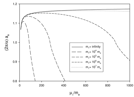
Figure 9: The anomalous moment of the electron in units of the Schwinger term (${\alpha/2\pi}$) [117] plotted versus the PV photon mass, $\mu_{1}$, for a few values of the PV electron mass, $m_{1}$, from [45]. The second PV photon flavor is absent, and the chiral symmetry of the massless limit is broken by the remaining regularization. The Fock-state expansion is truncated at one photon.

From Fig. 9, we see that, without the second PV photon, the PV electron mass needs to be on the order of $10^{7}\,m_{e}$ before results for the one-photon truncation approach the infinite-mass limit. Thus, the PV electron mass must be at least this large for a successful calculation with a two-photon Fock-space truncation, if only one PV photon flavor is included. Unfortunately, such large mass values make numerical calculations difficult, because of contributions to integrals at momentum fractions of order $(m_{e}/m_{1})^{2}\simeq 10^{-14}$, which are then subject to large round-off errors. Therefore, the two-photon calculation does require the second PV photon.

When the anomalous moment is re-calculated in the one-photon truncation with the second PV photon flavor included, the result is given in Fig. 10, for PV masses related by $\mu_{2}=\sqrt{2}\mu_{1}$.

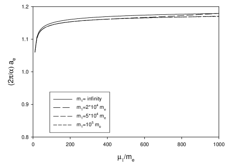
Figure 10: Same as Fig. 9, and also from [45], but with the second PV photon included, with a mass $\mu_{2}=\sqrt{2}\mu_{1}$, and the chiral symmetry is restored. The mass ratio is held fixed as $\mu_{1}$ and $\mu_{2}$ are varied.

Clearly, the dependence on the PV masses is greatly reduced.

The value obtained for the anomalous moment differs from the leading-order Schwinger result [117], and thus from the physical value, by 17%. This result is considerably improved if the self-energy contribution from the one-electron/two-photon Fock sector is included [20]. The alternative, sector-dependent renormalization method [17, 18] accomplishes this by restricting the bare mass in the one-electron/one-photon sector to being equal to the physical mass; however, this introduces the usual infrared divergence of perturbation theory which requires a nonzero photon mass and shifts the result for the anomalous moment away from the standard result [17].

The truncation of the dressed-electron state was extended to include two photons, and the anomalous moment was computed [82, 181]. With the chiral symmetry properly controlled, there is a plateau in the dependence on the PV mass, as shown in Fig. 11.

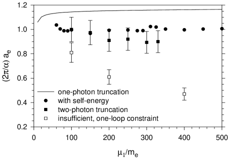
Figure 11: The anomalous moment of the electron in units of the Schwinger term ($\alpha/2\pi$) [117] plotted versus the PV photon mass, $\mu_{1}$, with the second PV photon mass, $\mu_{2}$, set to $\sqrt{2}\mu_{1}$ and the PV electron mass $m_{1}$ equal to $2\cdot 10^{4}\,m_{e}$, from [82]. The solid squares are the result of the full two-photon truncation with the correct, nonperturbative chiral constraint. The open squares come from use of a perturbative, one-loop constraint. Results for the one-photon truncation [45] (solid line) and the one-photon truncation with the two-photon self-energy contribution [20] (filled circles) are also included.

The main result for the two-photon truncation is in general agreement with experiment, within numerical errors. It is, however, systematically slightly below, due to the absence of two important contributions. One is from the Fock sector with an electron-positron loop, which contributes at the same order as the two-photon sector in perturbation theory, and the other is the three-photon self-energy contribution.

The work on QED has gone beyond Feynman gauge to include arbitrary covariant gauges [27]. The gauge dependence was checked for a one-photon/one-electron truncation of the Fock expansion for the dressed electron. The result for the anomalous moment is shown in Fig. 12.

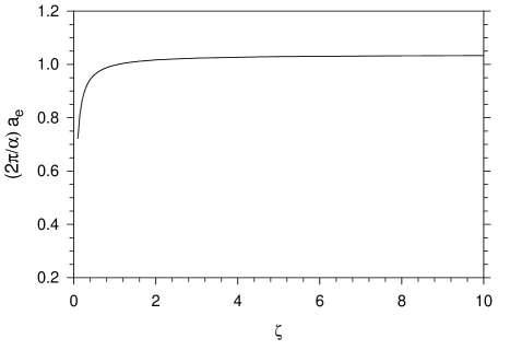
Figure 12: The anomalous magnetic moment $a_{e}$, relative to the Schwinger term $\alpha/2\pi$ [117], for the dressed-electron state truncated to include at most the one-electron/one-photon Fock states, as a function of the gauge parameter $\zeta$, with a bare photon mass of $\mu_{0}=0.001\,m_{e}$ and PV photon mass of $\mu_{1}=200\,m_{e}$, from [27].

The gauge parameter $\zeta$ is the coefficient of the gauge-fixing term in the Lagrangian; thus, $\zeta=0$ is a singular limit where the gauge fixing is removed and the theory is undefined. Except for values of $\zeta$ near 0, the anomalous moment varies only slightly. This variation is due to Fock-space truncation errors.

The one-photon truncation has also been solved with the BLFQ method [99, 100], both in a transverse cavity and as free (modeled as a weak cavity field). The dressed electron problem was formulated in light-cone gauge; however, the instantaneous interactions were neglected, making the coupled system for the wave functions very similar in structure to the Feynman-gauge system. The ultraviolet divergences were regulated by the basis choice and by the basis truncation. Sector-dependent mass renormalization was also used, with the physical electron mass assigned in the $|e\gamma\rangle$ sector and the bare mass in the $|e\rangle$ sector adjusted to yield the correct eigenmass for the dressed state. Without sector-dependent coupling renormalization, to absorb the uncanceled divergence from the broken Ward identity, the norm of the wave function diverges in the infinite basis limit, and results had to be extracted from a range of finite cutoffs. Later work argues for an explicit renormalization of the matrix element for the anomalous moment [182].

These investigations included careful studies of convergence with respect to both the basis size $N_{\rm max}$ and the oscillator energy scale $\Omega$. In the free case, convergence is slow because the harmonic oscillator basis functions are not a good match to the power-law behavior of the electron’s wave functions. However, the harmonic oscillator functions should be a good approximation for the confined quarks of QCD, and this work serves as test of the method. The results are comparable to the known perturbative result and the other nonperturbative calculations, as illustrated in Fig. 13.

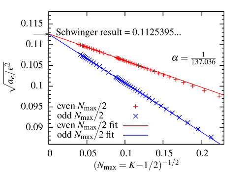
Figure 13: The square-root of the anomalous magnetic moment $a_{e}$, relative to the electron charge $e$, as a function of the BLFQ basis-size parameter $N_{\rm max}$, with resolution $K$ set to $N_{\rm max}+1/2$ and the oscillator-basis energy scale $b=m_{e}$, from [100]. The lines are from linear fits for $N_{\rm max}>150$.

As another illustration of the LFCC method, the dressed-electron state can be investigated [123]. To simplify the calculations, electron-positron pairs are excluded; however, an infinite number of photons is retained. The anomalous moment can then be computed from a spin-flip matrix element of the current. The valence state is the bare electron, and the $T$ operator is truncated to just simple photon emission from an electron:

$$T = \sum_{ijls\sigma\lambda}\int dyd\vec{k}_{\perp}\int\frac{d\underline{p}}{\sqrt{16\pi^{3}}}\sqrt{p^{+}}\,t_{ijl}^{\sigma s\lambda}(y,\vec{k}_{\perp})$$

$$\rule{72.26999pt}{0.0pt}\times a_{l\lambda}^{\dagger}(yp^{+},y\vec{p}_{\perp}+\vec{k}_{\perp})b_{js}^{\dagger}((1-y)p^{+},(1-y)\vec{p}_{\perp}-\vec{k}_{\perp})b_{i\sigma}(\underline{p}).$$

This includes as much physics as the two-photon Fock-space truncation considered earlier [82].

A graphical representation of the effective Hamiltonian $\overline{{\cal P}^{-}}$, excluding terms that annihilate the valence state, is given in Fig. 14.

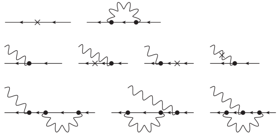
Figure 14: Graphical representation of the terms of the LFCC effective QED Hamiltonian. Each graph represents an operator that annihilates an electron and creates either a single electron or an electron and photon. The crosses indicate light-front kinetic-energy contributions.

The self-energy loop is the same in each contribution, without the sector and spectator dependence found in calculations with Fock-space truncation. Another consequence of using the LFCC method is that terms corresponding to all three graphs for the Ward identity in Fig. 2 appear in the effective Hamiltonian, as indicated by the last row of Fig. 14, which prevents the uncanceled divergence encountered in a Fock-space truncation. Also, in the equations for the functions $t_{ijl}^{\sigma s\lambda}(y,\vec{k}_{\perp})$, the physical mass of the eigenstate replaces the bare mass in the kinetic energy term, without use of sector-dependent renormalization [16, 17, 18, 20].

The anomalous moment $a_{e}=F_{2}(0)$ is obtained from the spin-flip matrix element of the current $J^{+}=\overline{\psi}\gamma^{+}\psi$ [40], coupled to a photon of momentum $q$ in the Drell–Yan ($q^{+}=0$) frame [41], as given in Eq. (52). The formalism for a projected expectation value [123], with the projection $P_{s}$ being the projection onto the physical subspace with the two transverse polarizations $\lambda=1,2$, yields for the current matrix element

$$\langle\psi_{a}^{\sigma}(\underline{P}+\underline{q})|J^{+}(0)|\psi_{a}^{\pm}(\underline{P})\rangle=\frac{\langle\widetilde{\psi}_{a}^{\sigma}(\underline{P}+\underline{q})|e^{-T}P_{s}^{\dagger}J^{+}(0)P_{s}e^{T}|\phi_{a}^{\pm}(\underline{P})\rangle}{\int d\underline{P}^{\prime}\langle\widetilde{\psi}_{a}^{\pm}(\underline{P}^{\prime})|e^{-T}P_{s}^{\dagger}P_{s}e^{T}|\phi_{a}^{\pm}(\underline{P})\rangle},$$ (237)

with $\langle\widetilde{\psi}_{a}^{\sigma}(\underline{P}+\underline{q})|$ the left-hand eigenstate of $\overline{{\cal P}^{-}}$

$$|\widetilde{\psi}_{a}^{\pm}(\underline{P})\rangle=|\tilde{\phi}_{a}^{\pm}(\underline{P})\rangle$$

$$+\sum_{jls\lambda}\int dyd\vec{k}_{\perp}\sqrt{\frac{P^{+}}{16\pi^{3}}}l_{ajl}^{\pm s\lambda}(y,\vec{k}_{\perp})a_{l\lambda}^{\dagger}(yP^{+},y\vec{P}_{\perp}+\vec{k}_{\perp})b_{js}^{\dagger}((1-y)P^{+},(1-y)\vec{P}_{\perp}-\vec{k}_{\perp})|0\rangle,$$

The truncation to $|e\rangle+|e\gamma\rangle$ is consistent with the truncation of $T$. The form factors can then be extracted.

This can be checked by considering the perturbative solutions for the right and left-hand wave functions; substitution into the expression for $a_{e}$ gives immediately the Schwinger result [117] of $\alpha/2\pi$, in the limit of zero photon mass, for any covariant gauge [123]. A complete calculation requires a numerical solution of the eigenvalue problems. This will yield all contributions to $a_{e}$ of order $\alpha^{2}$, except those with electron-positron pairs, and a partial summation of higher orders.

4.5.2 positronium

The first application of light-front techniques to positronium in light-cone gauge was by Tang et al. [173]. An improved treatment of the Coulomb singularity led to better convergence [174]. Both of these attempts considered an effective interaction in the $|e^{+}e^{-}\rangle$ sector, with the $|e^{+}e^{-}\gamma\rangle$ sector integrated out and all other sectors neglected. A direct diagonalization of the light-front QED Hamiltonian was attempted by Kaluža and Pauli [175]. This work culminated in the more exhaustive study by Trittmann and Pauli [176], which included the annihilation channel and numerical convergence to restoration of rotational invariance; the light-front equations were discretized by Gauss-Legendre quadrature.

More recently, the BLFQ method has been used to study positronium [101], again in light-cone gauge, with a Fock-space truncation to the $|e^{+}e^{-}\rangle$ and $|e^{+}e^{-}\gamma\rangle$ sectors. The annihilation channel, with coupling to the $|\gamma\rangle$ sector, is not included. With use of the Bloch formalism  [183], the higher sector is eliminated to yield an effective one-photon-exchange interaction in the lower sector, and the self-energy contributions neglected. This is equivalent to the truncations made for the earlier work [174, 176], but the numerical approximation is quite different. More important, it will serve as a point of reference for future calculations with self-energies and sector-dependent renormalization.

If the full Hamiltonian were used instead of the Bloch-reduced Hamiltonian, the matrix representation would be much larger but much more sparse. However, the self-energy terms would be automatically included with no simple way to exclude them. Of course, eventually this is exactly what needs to be considered, to approximate the full many-body problem. This will require a better understanding of the renormalization generated by the self-energy corrections.

The calculation is done at $\alpha=0.3$, in order to make higher-order effects visible numerically. The results compare quite favorably with those from the Schrödinger equation with (perturbative) relativistic corrections, to order $\alpha^{4}$. The dependence on the regulators and the rate of convergence were thoroughly studied. The convergence rate with respect to the basis cutoff $N_{\rm max}$ was found to be strongly affected by the choice of oscillator energy scale $b$; the convergence rate with respect to the longitudinal DLCQ resolution $K$ was affected by the photon mass $\mu$.

The convergence is again slow, because harmonic oscillator functions are not the best approximation to the exponential functions of the Schrödinger-Coulomb problem. However, as preparation for the calculation of meson states, the use of oscillator functions is worthwhile. Similarly, though the two-body sector lends itself to solution in terms of relative coordinates, the single-particle basis set of BLFQ was retained, as preparation for calculations that include more Fock sectors explicitly.

The instantaneous-photon interaction is singular for small longitudinal photon momentum. In a perturbative calculation, this is canceled by a contribution from regular photon exchange, which can be matched term by term. In the nonperturbative calculation, the cancellation is not complete and requires a counterterm. Similar counterterms were used in earlier work [174, 176], where extensive discussion of this counterterm can be found.

The integrable Coulomb singularity, while controlled in principle, causes difficulties numerically. A photon mass is introduced to regulate it.

There is also a logarithmic divergence from the one-photon-exchange kernel [174, 184] that requires a counterterm. This takes into account effects of the (missing) $|e^{+}e^{-}\gamma\gamma\rangle$ sector. Unfortunately, the counterterm worsens the breaking of rotational symmetry.

The Fock-sector truncation and the asymmetry between the longitudinal and transverse discretizations destroy the rotational invariance of the Hamiltonian. Thus, the $M_{J}$ multiplets are not degenerate. However, the individual projections are typically close enough to allow assignment of $J$ values.

4.5.3 true muonium

The general approach used for positronium can be naturally extended to analyze true muonium, the bound states of the $\mu^{+}$-$\mu^{-}$ system. These states are metastable, with lifetimes short compared to the muon lifetime. The methods of [176] have been extended to true muonium by Lamm and Lebed [80]. They include $|\mu^{+}\mu^{-}\rangle$ and $|e^{+}e^{-}\rangle$ sectors and effective interactions obtained by integrating out the one-photon annihilation channel and the higher sectors with an added photon. The impact of the $|e^{+}e^{-}\rangle$ component is investigated by allowing the electron mass to be comparable to the muon mass. The coupling strength is again held at $\alpha=0.3$.

The numerical methods were based on Clenshaw–Curtis [185] and Gauss-Chebyshev quadratures. The Coulomb singularity required different counterterms in each sector. In general, the cutoff dependence and choice of counterterms are studied carefully, leading to good agreement with nonrelativistic calculations that include relativistic effects perturbatively. The agreement provides confirmation that the light-front calculations are done correctly. However, one must keep in mind that these and other tests of light-front methods in QED are just that, tests of the method, and will never be competitive with equal-time calculations. The true home of light-front methods is in strongly interacting theories where perturbative corrections of some zero-order (non)relativistic approximation cannot be used effectively.

4.6 Quantum Chromodynamics

Two-dimensional QCD has been studied quite extensively in the DLCQ approximation [186]. The earliest application to four-dimensional QCD is a DLCQ calculation by Hollenberg et al. [187]; however, such four-dimensional applications have lacked a consistent regularization. The various methods developed since, such as PV regularization [28, 188] and sector-dependent renormalization should provide a path forward. The primary purpose of this review is to facilitate and encourage progress along that path.

As an alternative to direct diagonalization of the QCD Hamiltonian, one can use light-front techniques to construct and analyze quark models, particularly in parallel with the AdS/QCD approach [105]. The BLFQ method has been modified to use relative coordinates and study heavy quarkonium in exactly this way [189]. This allows the calculation of masses and decay constants. McCartor and Dalley [190] have derived an effective Hamiltonian operator to induce chiral symmetry breaking; this could be incorporated into a study of mesons in QCD. There is also a construction of a confining interaction based on the requirement of restoration for rotational symmetry [191, 192, 193].

Glueball states have been studied [194] with a renormalized light-front Hamiltonian, constructed from recursion relations that restore symmetries and eliminate cutoff dependence. The Fock space was truncated to the two-gluon sector, and the Hamiltonian provided an effective interaction to bind the gluons. The renormalization scheme was developed in the context of scalar theories [195, 196] and builds on the fundamental ideas of Wilson et al. [31, 30] for a derivation of the constituent quark model from light-front QCD. Along similar lines, asymptotic freedom in pure-glue QCD has been investigated with the related RGPEP [197].

5 Future Challenges

The preceding sections have provided an in-depth review of the nonperturbative methods applied to light-front calculations in a variety of quantum field theories. In each case, there remain many interesting questions to pursue, not the least of which, of course, is the solution of QCD itself, and there are many other applications not yet considered.

For quenched scalar Yukawa theory, perhaps the most important open question is the convergence of the LFCC method. This theory is the simplest theory for such a test, because the $T$ operator has the simplest possible form, and the theory is not very far removed from the simple model where the leading LFCC approximation gives the exact solution [21]. Another important question to be understood is why sector-dependent renormalization works so well for calculations with Fock-space truncation [134], seemingly avoiding the pitfalls found in Yukawa theory and QED [20]. Is the boson nature of the theory the key? In which case, does this bode well for the gluons of QCD?

This leads to the more general question of whether sector-dependent renormalization can be interpreted in some way to allow meaningful calculations. The triviality limit on cutoffs [148, 20] must somehow be absorbed into the rules for extraction of physical observables. Avoidance of Fock-space truncation, via the LFCC method, may be the best route forward, but the work on quenched scalar Yukawa theory [134] indicates that Fock-space truncation and sector-dependent renormalization may also provide a useful set of rules for calculation.

In $\phi^{4}_{1+1}$ theory, the standard bearer for theories with broken symmetry, there is still much to consider, if only to show that light-front methods can do as good a job as any other approach. Specifically, the critical couplings and critical exponents should be calculable for the restoration of symmetry in the negative-mass-squared case as well as for the dynamical symmetry breaking in both the positive and negative mass-squared cases. However, any comparison with equal-time calculations that is done in terms of bare parameters must take into account the different renormalizations [137]. Near the critical coupling, where the mass of the dressed state is close to zero and the probabilities of higher Fock states should be large, use of sector-dependent mass renormalization or the LFCC method is probably crucial.

Zero modes can be useful in the analysis of $\phi^{4}$ theory but are not necessarily required [57]. In any case, much hinges on the interpretation of the Fock vacuum $|0\rangle$. Critical couplings are typically signaled by degeneracy of a dressed eigenstate with the (massless) vacuum. An increase of the coupling beyond this point drives the “massive” eigenstate below zero and therefore below the alleged vacuum, a nonsensical outcome. This implies that the quantization has been done incorrectly; the Fock vacuum should always be the lowest state. A correct quantization should either shift the field explicitly [70] or introduce zero modes that give some structure to the vacuum. Either way, the field then develops the necessary vacuum expectation value.

The solution of Yukawa theory should be carried out with an additional PV scalar, to nonperturbatively restore the chiral symmetry of the massless limit. The work on Yukawa theory was done [81, 19] before the understanding of the symmetry restoration was achieved in the context of PV-regulated QED.

The work on supersymmetric Yang–Mills theory should be extended to 3+1 dimensions. This would bring the possibility of analyzing QCD as a limit of supersymmetric QCD, with the superpartners replacing PV fields as the regulators. Obviously, this also entails supersymmetry breaking, to give the superpartners a large mass. However, this is distinct from supersymmetric extensions of the Standard Model, which are theories in their own right. Instead, the idea is to use supersymmetry as a regularization tool, with no physical interpretation given to the superpartners, which would be removed from the calculation in an infinite-mass limit. The limitations on the form of supersymmetry breaking, that come from the appearance of unobserved processes such as flavor-changing decays, would not necessarily be applicable, which broadens the options for the mechanism of the breaking.

For both Yukawa theory and QED, very little has been done on the inclusion of vacuum polarization [108]. Typically, the Fock space is truncated to exclude additional fermion-antifermion pairs. This leaves open the question of nonperturbative charge renormalization. The charge renormalization done in sector-dependent renormalization is ‘only’ an artifact of absorbing wave function and vertex renormalization, leftover from a broken Ward identity. Of course, the LFCC method sidesteps issues of Fock-space truncation, but needs to be tested in both Yukawa theory and QED.

There is a similar renormalization issue in the treatment of self-energy corrections for multiparticle bound states. Calculations have typically divided into two types. One type focuses on the dressing of a single particle; here self-energies are the center of the piece. The other type focuses on binding two constituents, usually by an effective interaction obtained by integrating out other Fock sectors; here self-energies are explicitly neglected, to understandably simplify the calculation. In the future, the knowledge gained from the first type needs to be merged with the second. This is particularly important before moving on to less severe Fock-space truncations for which a reduction to a single effective equation and identification of self-energy contributions cannot be done. The LFCC method should be useful because there the self-energy corrections tend to be spectator independent.

Simply by measuring the length of the section on applications to QCD in comparison with the length of the other sections, one can see that there is much to be done. However, many if not all of the tools necessary for the job have been established. Nonperturbative calculations of simpler systems such as glueballs and heavy mesons are within reach. The potential for an explanation of confinement is particularly interesting in these systems, perhaps based on RGPEP [29] or the LFCC method; in the latter method, an infinite number of gluons can be included.

There is also much formal work to be done. A proof of renormalizability is needed for the proposed PV regularization scheme [28]. A small step in this direction is the introduction of Nakanishi–Lautrup fields [198] to make the BRST transformation nilpotent off-shell. However, there are more than just the usual complications of perturbative renormalization, because, after all, the objective is use in a nonperturbative calculation. The philosophy employed so far has been that a regularization adequate for perturbation theory is then sufficient for nonperturbative calculations, implicitly assuming that renormalizability carries over as well. This may not be the case; for example, in any gauge-fixed theory, one must contend with the existence of Gribov copies [199].

Nevertheless, the time is ripe for tremendous progress in light-front solutions for systems in QCD. Consider the progress that lattice gauge theory has made in the twenty-five years since its originator expressed so much pessimism [13]. This progress was accomplished through the concerted and combined efforts of a large community. The challenge of the future is for light-front methods to be carried forward in just such a manner.

References

- [1] P.A.M. Dirac, Rev. Mod. Phys. 21 (1949) 392
- [2] S.J. Brodsky, H.-C. Pauli, and S.S. Pinsky, Phys. Rep. 301 (1998) 299
- [3] J. Carbonell, B. Desplanques, V.A. Karmanov, and J.F. Mathiot, Phys. Rep. 300 (1998) 215
- [4] G.A. Miller, Prog. Part. Nucl. Phys. 45 (2000) 83
- [5] M. Burkardt, Adv. Nucl. Phys. 23 (2002) 1
- [6] B.L.G. Bakker et al., Nucl. Phys. Proc. Suppl. 251-252 (2014) 165
- [7] C. Gattringer and C.B. Lang, Quantum Chromodynamics on the Lattice (Springer, Berlin, 2010); H. Rothe, Lattice Gauge Theories: An Introduction, 4e (World Scientific, Singapore, 2012)
- [8] C.D. Roberts and A.G. Williams, Prog. Part. Nucl. Phys. 33 (1994) 477 ; C.D. Roberts and S.M. Schmidt, Prog. Part. Nucl. Phys. 45 (2000) S1 ; R. Alkofer and L. von Smekal, Phys. Rep. 353 (2001) 281 ; P. Maris and C.D. Roberts, Int. J. Mod. Phys. E 12 (2003) 297 ; C.S. Fischer, J. Phys. G 32 (2006) R253 ; C.D. Roberts, M.S. Bhagwat, A. Holl and S.V. Wright, Eur. Phys. J. ST 140 (2007) 53 ; I. C. Cloet and C. D. Roberts, Prog. Part. Nucl. Phys. 77 (2014) 1
- [9] M. Hogervorst, S. Rychkov and B. C. van Rees, Phys. Rev. D 91 (2015) 025005
- [10] M. Burkardt and S. Dalley, Prog. Part. Nucl. Phys. 48 (2002) 317 ; S. Dalley and B. van de Sande, Phys. Rev. D 67 (2003) 114507 ; D. Chakrabarti, A.K. De, and A. Harindranath, Phys. Rev. D 67 (2003) 076004 ; M. Harada and S. Pinsky, Phys. Lett. B 567 (2003) 277 ; for work on a complete light-cone lattice, see C. Destri and H.J. de Vega, Nucl. Phys. B 290 (1987) 363 ; D. Mustaki, Phys. Rev. D 38 (1989) 1260
- [11] C. Cruz-Santiago, P. Kotko, and A.M. Staśto, Prog. Part. Nucl. Phys. 85 (2015) 82
- [12] H.-C. Pauli and S.J. Brodsky, Phys. Rev. D 32 (1985) 1993 ; Phys. Rev. D 32 (1985) 2001
- [13] K.G. Wilson, Nucl. Phys. BProc. Suppl. 17 (1990) 82
- [14] J.P. Vary, H. Honkanen, J. Li, P. Marix, S.J. Brodsky, A Harindranath, G.F. de Teramond, P. Sternberg, E.G. Ng, and C. Yang, Phys. Rev. C 81 (2010) 035205
- [15] S.S. Chabysheva and J.R. Hiller, Phys. Rev. D 88 (2013) 085006
- [16] R.J. Perry, A. Harindranath, and K.G. Wilson, Phys. Rev. Lett. 65 (1990) 2959 ; R.J. Perry and A. Harindranath, Phys. Rev. D 43 (1991) 4051
- [17] J.R. Hiller and S.J. Brodsky, Phys. Rev. D 59 (1998) 016006
- [18] V.A. Karmanov, J.-F. Mathiot, and A.V. Smirnov, Phys. Rev. D 77 (2008) 085028
- [19] V.A. Karmanov, J.-F. Mathiot, and A.V. Smirnov, Phys. Rev. D 82 (2010) 056010
- [20] S.S. Chabysheva and J.R. Hiller, Ann. Phys. (N.Y.) 325 (2010) 2435
- [21] S.S. Chabysheva and J.R. Hiller, Phys. Lett. B 711 (2012) 417
- [22] W. Pauli and F. Villars, Rev. Mod. Phys. 21 (1949) 434
- [23] G. ’t Hooft and M. Veltman, Nucl. Phys. B 44 (1972) 189 ; C.G. Bollini and J.J. Giambiagi, Phys. Lett. B 40 (1972) 566 ; J.F. Ashmore, Nuovo Cim. Lett. 4 (1972) 289
- [24] S.J. Brodsky, V.A. Franke, J.R. Hiller, G. McCartor, S.A. Paston, and E.V. Prokhvatilov, Nucl. Phys. B 703 (2004) 333
- [25] B. L. G. Bakker, J. K. Boomsma and C. R. Ji, Phys. Rev. D 75 (2007) 065010
- [26] C. Becchi, A. Rouet, and R. Stora, Phys. Lett. B 52 (1974) 344 ; Commun. Math. Phys. 42 (1975) 127 ; Ann. Phys. (N.Y.) 98 (1976) 287 ; I.V. Tyutin IV Lebedev preprint FIAN No. 39, (1975) unpublished
- [27] S.S. Chabysheva and J.R. Hiller, Phys. Rev. D 84 (2011) 034001
- [28] S.S. Chabysheva and J.R. Hiller, arXiv:1506.05429
- [29] S.D. Glazek, Phys. Rev. D 85 (2012) 125018 ; Phys. Rev. D 87 (2013) 125032
- [30] R. J. Perry, Ann. Phys. (N.Y.) 232 (1994) 116
- [31] K. G. Wilson, T. S. Walhout, A. Harindranath, W. M. Zhang, R. J. Perry and S. D. Glazek, Phys. Rev. D 49 (1994) 6720
- [32] S.D. Glazek and K.G. Wilson, Phys. Rev. D 48 (1993) 5863 ; Phys. Rev. D 49 (1994) 4214
- [33] O. Lunin and S. Pinsky, AIP Conf. Proc. 494 (1999) 140 ; Y. Matsumura, N. Sakai, and T. Sakai, Phys. Rev. D 52 (1995) 2446
- [34] S.S. Chabysheva and J.R. Hiller, Phys. Rev. E 90 (2014) 063310 ; S.S. Chabysheva, B. Elliott, and J.R. Hiller, Phys. Rev. E 88 (2013) 063307
- [35] M. Burkardt and A. Langnau, Phys. Rev. D 44 (1991) 3857 ; C. R. Ji, G. H. Kim and D. P. Min, Phys. Rev. D 51 (1995) 879 ; J. R. Cooke, G. A. Miller and D. R. Phillips, Phys. Rev. C 61 (2000) 064005 ; B. L. G. Bakker, M. A. DeWitt, C. R. Ji and Y. Mishchenko, Phys. Rev. D 72 (2005) 076005
- [36] E.C.G. Stueckelberg, Helv. Phys. Acta 11 (1938) 225 ; F. Coester, Phys. Rev. 83 (1951) 798
- [37] S.N. Gupta, Proc. Phys. Soc. (London) A63 (1950) 681 ; K. Bleuler, Helv. Phys. Acta 23 (1950) 567
- [38] M. Herrmann and W.N Polyzou, Phys. Rev. D 91 (2015) 085043
- [39] L. Martinovic, Phys. Lett. B 400 (1997) 335 ; L. Martinovic and J.P. Vary, Phys. Rev. D 64 (2001) 105016 ; L. Martinovic, Phys. Rev. D 78 (2008) 105009 ; L. Martinovic and P. Grange, Mod. Phys. Lett. A 23 (2008) 417 ; Phys. Lett. B 724 (2013) 310
- [40] S.J. Brodsky and S.D. Drell, Phys. Rev. D 22 (1980) 2236
- [41] S.D. Drell, D.J. Levy, and T.M. Yan, Phys. Rev. Lett. 22 (1969) 744
- [42] M. Diehl, Phys. Rep. 388 (2003) 41 ; A.V. Belitsky and A.V. Radyushkin, Phys. Rep. 418 (2005) 1 ; K. Goeke, M.V. Polyakov, and M. Vanderhaeghen, Prog. Part. Nucl. Phys. 47 (2005) 401 ; S. Boffi and B. Pasquini, Riv. Nuovo Cimento 30 (2007) 387
- [43] D. Chakrabarti, X. Zhao, H. Honkanen, R. Manohar, P. Maris, and J.P. Vary, Phys. Rev. D 89 (2014) 116004
- [44] S.J. Brodsky, R. Roskies, and R. Suaya, Phys. Rev. D 8 (1973) 4574
- [45] S.S. Chabysheva and J.R. Hiller, Phys. Rev. D 79 (2009) 114017
- [46] H. M. Choi and C. R. Ji, Phys. Rev. D 58 (1998) 071901
- [47] J. P. B. C. de Melo, T. Frederico, H. W. L. Naus and P. U. Sauer, Nucl. Phys. A 660 (1999) 219 ; B. L. G. Bakker, H. M. Choi and C. R. Ji, Phys. Rev. D 65 (2002) 116001
- [48] S. Elser and A.C. Kalloniatis, Phys. Lett. B 375 (1996) 285
- [49] A. Harindranath and J.P. Vary, Phys. Rev. D 37 (1988) 3010 ; E.A. Bartnik and S.D. Glazek, Phys. Rev. D 39 (1989) 1249
- [50] T. Almeida, V.S. Alves, D.T. Alves, S. Perez, and P.L.M. Rodrigues, Phys. Rev. D 87 (2013) 065028
- [51] F. Lenz and D. Steinbacher, Phys. Rev. D 67 (2003) 045010
- [52] J.R. Hiller, Y. Proestos, S. Pinsky, and Salwen, Phys. Rev. D 70 (2004) 065012 ; J.R. Hiller, S. Pinsky, Y. Proestos, N. Salwen, and U. Trittmann, Phys. Rev. D 76 (2007) 045008
- [53] S. Strauss and M. Beyer, Phys. Rev. Lett. 101 (2008) 100402
- [54] S. Strauss, S. Mattiello and M. Beyer, J. Phys. G 36 (2009) 085006
- [55] T. Maskawa and K. Yamawaki, Prog. Theor. Phys. 56 (1976) 270
- [56] J. R. Hiller, S. Pinsky, Y. Proestos, N. Salwen, and U. Trittmann, Phys. Rev. D 76 (2007) 045008
- [57] J.S. Rozowsky and C.B. Thorn, Phys. Rev. Lett. 85 (2000) 1614
- [58] V.T. Kim, G.B. Pivovarov, and J.P. Vary, Phys. Rev. D 69 (2004) 085008
- [59] D. Chakrabarti, A. Harindranath, L. Martinovic, G. B. Pivovarov, and J. P. Vary, Phys. Lett. B 617 (2005) 92
- [60] D. Chakrabarti, A. Harindranath, L. Martinovic, and J. P. Vary, Phys. Lett. B 582 (2004) 196
- [61] D. Chakrabarti, A. Harindranath and J. P. Vary, Phys. Rev. D 71 (2005) 125012
- [62] A. Harindranath and J.P. Vary, Phys. Rev. D 37 (1988) 1064
- [63] A. Harindranath and J.P. Vary, Phys. Rev. D 36 (1987) 1141 ; Phys. Rev. D 37 (1988) 1076
- [64] A. Harindranath and J.P. Vary, Phys. Rev. D 37 (1988) 3010
- [65] T. Eller, H.-C. Pauli, and S.J. Brodsky, Phys. Rev. D 35 (1987) 1493
- [66] M. Burkardt, Nucl. Phys. A 504 (1989) 762 ; K. Hornbostel, S.J. Brodsky, and H.-C. Pauli, Phys. Rev. D 41 (1990) 3814
- [67] I. Tamm, J. Phys. (Moscow) 9 (1945) 449 ; S.M. Dancoff, Phys. Rev. 78 (1950) 382
- [68] Th. Heinzl, St. Krusche, and E. Werner, Phys. Lett. B 272 (1991) 54 ; Phys. Lett. B 275 (1992) 410 ; T. Heinzl, S. Krusche, S. Simburger, and E. Werner, Z. Phys. C 56 (1992) 415
- [69] D.G. Robertson, Phys. Rev. D 47 (1993) 2549
- [70] K. Hornbostel, Phys. Rev. D 45 (1992) 3781
- [71] C.M. Bender, S.S. Pinsky, and B. van de Sande, Phys. Rev. D 48 (1993) 816 ; S.S. Pinsky and B. van de Sande, Phys. Rev. D 49 (1994) 2001 ; S.S. Pinsky, B. van de Sande, and J.R. Hiller, Phys. Rev. D 51 (1995) 726
- [72] A. Borderies, P. Grangé, and E. Werner, Phys. Lett. B 319 (1993) 490 ; Phys. Lett. B 345 (1995) 458 ; P. Grangé, P. Ullrich, and E. Werner, Phys. Rev. D 57 (1998) 4981 ; S. Salmons, P. Grangé, and E. Werner, Phys. Rev. D 60 (1999) 067701 ; S. Salmons, P. Grangé, and E. Werner, Phys. Rev. D 65 (2012) 125014
- [73] J.J. Wivoda and J.R. Hiller, Phys. Rev. D 47 (1993) 4647
- [74] M. Maeno, Phys. Lett. B 320 (1994) 83
- [75] S.S. Chabysheva and J.R. Hiller, Phys. Rev. D 79 (2009) 0906012
- [76] S. Hellerman and J. Polchinski, Phys. Rev. D 59 (1999) 125002
- [77] M. Taniguchi, S. Uehara, S. Yamada, and K. Yamawaki, Mod. Phys. Lett. A 16 (2001) 2177 ; T. Heinzl, arXiv:hep-th/0310165
- [78] S. J. Brodsky, J. R. Hiller and G. McCartor, Phys. Rev. D 58 (1998) 025005
- [79] U. Trittmann and H.-C. Pauli, hep-th/9704215
- [80] H. Lamm and R.F. Lebed, J. Phys. G 41 (2014) 125003
- [81] S. J. Brodsky, J. R. Hiller and G. McCartor, Ann. Phys. (N.Y.) 321 (2006) 1240
- [82] S.S. Chabysheva and J.R. Hiller, Phys. Rev. D 81 (2010) 074030
- [83] I. Filippov, S.S. Pinsky, and J.R. Hiller, Phys. Lett. B 506 (2001) 221
- [84] M. Burkardt, F. Antonuccio, and S. Tsujimaru, Phys. Rev. D 58 (1998) 125005
- [85] J.R. Hiller, S.S. Pinsky, and U. Trittmann, Nucl. Phys. B 661 (2003) 99 ; Phys. Rev. D 67 (2003) 115005
- [86] F. Antonuccio, O. Lunin, S. Pinsky, and A. Hashimoto, JHEP 07 (1999) 029
- [87] J.R. Hiller, O. Lunin, S. Pinsky, and U. Trittmann, Phys. Lett. B 482 (2000) 409
- [88] C. Lanczos, J. Res. Nat. Bur. Stand. 45 (1950) 255 ; J.H. Wilkinson, The Algebraic Eigenvalue Problem (Clarendon, Oxford, 1965); B.N. Parlett, The Symmetric Eigenvalue Problem (Prentice–Hall, Englewood Cliffs, NJ, 1980); J. Cullum and R.A. Willoughby, in Large-Scale Eigenvalue Problems, eds. J. Cullum and R.A. Willoughby, Math. Stud. 127 (Elsevier, Amsterdam, 1986), p. 193; D.S. Scott, in Sparse Matrices and their Uses, edited by I.S. Duff (Academic Press, London, 1981), p. 139; G.H. Golub and C.F. van Loan, Matrix Computations (Johns Hopkins University Press, Baltimore, 1983); R.G. Grimes et al., J. Comput. Phys. 69 (1987) 471 ; R.G. Grimes and H.D. Simon, J. Comput. Phys. 77 (1988) 270 ; D.S. Scott, Comput. Phys. Commun. 53 (1989) 271
- [89] R. Haydock, in Solid State Physics, Vol. 35, edited by H. Ehrenreich, F. Seitz, and D. Turnbull, (Academic, New York, 1980), p. 283; W.H. Miller and B.M.D.D. Jansen op de Haar, J. Chem. Phys. 86 (1987) 6213 ; C. Duneczky and R.E. Wyatt, J. Chem. Phys. 89 (1988) 1448 ; C. Duneczky and R.E. Wyatt, J. Phys. B21 (1988) 3727 ; C.M.M. Nex, Comput. Phys. Commun. 53 (1989) 141 ; C. Duneczky et al., Comput. Phys. Commun. 53 (1989) 357 ; W. Yang and W.H. Miller, J. Chem. Phys. 91 (1989) 3504 ; H.D. Meyer and S. Pal, J. Chem. Phys. 91 (1989) 6195 ; H.D. Meyer, J. Horáček, and L.S. Cederbaum, Phys. Rev. A 43 (1991) 3587 ; J.R. Hiller, Phys. Rev. D 43 (1991) 2418 ; T.J. Godin and R. Haydock, Comput. Phys. Commun. 64 (1991) 123
- [90] S. Pissanetzky Sparse matrix technology (London, Academic Press, 1984)
- [91] J. Cullum and R.A. Willoughby, J. Comput. Phys. 44 (1981) 329 ; Lanczos Algorithms for Large Symmetric Eigenvalue Computations (Birkhauser, Boston, 1985), Vol. I and II
- [92] Y. Saad, Comput. Phys. Commun. 53 (1989) 71 ; S.K. Kin and A.T. Chronopoulos, J. Comp. and Appl. Math 42 (1992) 357
- [93] W. Pauli, Rev. Mod. Phys. 15 (1943) 175
- [94] S. J. Brodsky, J. R. Hiller and G. McCartor, Phys. Rev. D 64 (2001) 114023
- [95] R. Alben, M. Blume, H. Krakauer, and L. Schwartz, Phys. Rev. B 12 (1975) 4090 ; A. Hams and H. De Raedt, Phys. Rev. E 62 (2000) 4365
- [96] T. Iitaka and T. Ebisuzaki, Phys. Rev. E 69 (2004) 057701
- [97] J. Jaklič and P. Prelovšek, Phys. Rev. B 49 (1994) 5065(R) ; M. Aichhorn, M. Daghofer, H. G. Evertz, and W. von der Linden, Phys. Rev. B 67 (2003) 161103(R)
- [98] T.Z. Kalamboukis, J. Comp. Phys. 53 (1984) 82
- [99] H. Honkanen, P. Maris, J.P. Vary, and S.J. Brodsky, Phys. Rev. Lett. 106 (2011) 061603
- [100] X. Zhao, H. Honkanen, P. Maris, J.P. Vary, and S.J. Brodsky, Phys. Lett. B 737 (2014) 65
- [101] P. Wiecki, Y. Li, X. Zhao, P. Maris, and J.P. Vary, Phys. Rev. D 91 (2015) 105009
- [102] P. Navratil, J.P. Vary, and B.R. Barrett, Phys. Rev. Lett. 84 (2000) 5728 ; Phys. Rev. C 62 (2000) 054311 ; P. Maris, J.P. Vary, and A.M Shirokov, Phys. Rev. C 79 (2009) 014308
- [103] P.Maris, P.W. Wiecki, Y. Li, X. Zhao, and J.P. Vary, Acta Phys. Pol. B Proc. Suppl. 6 (2013) 321
- [104] D.H. Bloeckner and R.D. Lawson, Phys. Lett. B 53 (1974) 313
- [105] S. J. Brodsky, G. F. de Teramond, H. G. Dosch, and J. Erlich, Phys. Rep. 584 (2015) 1
- [106] X. Zhao, A. Ilderton, P. Maris, and J.P. Vary, Phys. Lett. B 726 (2013) 856 ; Phys. Rev. D 88 (2013) 065014
- [107] T.D. Lee and G.C. Wick, Nucl. Phys. B 9 (1969) 209 ; Phys. Rev. D 2 (1972) 1033 ; B. Grinstein, D. O’Connell, and M.B. Wise, Phys. Rev. D 77 (2008) 025012 ; C.D. Carone and R.F. Lebed, Phys. Lett. B 668 (2008) 221 ; JHEP 0901 (2009) 043
- [108] S.S. Chabysheva and J.R. Hiller, Phys. Rev. D 82 (2010) 034004
- [109] S.J. Brodsky, J.R. Hiller, and G. McCartor, Ann. Phys. (N.Y.) 305 (2003) 266
- [110] P.T. Matthews, Phys. Rev. 76 (1949) 1254 ; A. Salam, Nucl. Phys. 18 (1960) 681 S. Kamefuchi, Nucl. Phys. 18 (1960) 691
- [111] E.C.G. Stueckelberg, Helv. Phys. Acta 11 (1938) 299 ; Helv. Phys. Acta 11 (1938) 312
- [112] R. Marnelius and I.S. Sogami, Int. J. Mod. Phys. A 13 (1998) 3101
- [113] L.D. Faddeev and V.N. Popov, Phys. Lett. B 25 (1967) 29
- [114] A. Grozin, Lectures on QED and QCD, (World Scientific, Singapore, 2007)
- [115] D. Bailin and A. Love, Introduction to Gauge Field Theory (Institute of Physics, Bristol, 1993)
- [116] D. Mustaki, S. Pinsky, J. Shigemitsu, and K. Wilson, Phys. Rev. D 43 (1991) 3411
- [117] J. Schwinger, Phys. Rev. 73 (1948) 416 ; Phys. Rev. 76 (1949) 790
- [118] S.S. Chabysheva and J.R. Hiller, Ann. Phys. (N.Y.) 340 (2014) 188
- [119] A. Misra, Phys. Rev. D 50 (1994) 4088 ; Phys. Rev. D 53 (1996) 5874 ; Phys. Rev. D 62 (2000) 125017 ; L. Martinovic, Phys. Lett. B 400 (1997) 335 ; L. Martinovic and J.P. Vary, Phys. Lett. B 459 (1999) 186 ; J.D. More and A. Misra, Phys. Rev. D 86 (2012) 065037 ; Phys. Rev. D 87 (2013) 085035 ; Phys. Rev. D 89 (2014) 105021
- [120] F. Coester, Nucl. Phys. 7 (1958) 421 ; F. Coester and H. Kümmel, Nucl. Phys. 17 (1960) 477
- [121] For reviews of the many-body coupled-cluster method, see R.J. Bartlett and M. Musial, Rev. Mod. Phys. 79 (2007) 291 ; T.D. Crawford, and H.F. Schaefer, Rev. Comp. Chem. 14 (2000) 33 ; R. Bishop, A.S. Kendall, L.Y. Wong, and Y. Xian, Phys. Rev. D 48 (1993) 887 ; H. Kümmel, K.H. Lührmann, and J.G. Zabolitzky, Phys. Rep. 36 (1978) 1
- [122] M. Funke and H.G. Kümmel, Phys. Rev. D 50 (1994) 991 ; A.H. Rezaeian and N.R. Walet, JHEP 0312 (2003) 040 ; Phys. Lett. B 570 (2003) 129
- [123] S.S. Chabysheva and J.R. Hiller, arXiv:1203.0250
- [124] G.C. Wick, Phys. Rev. 96 (1954) 1124 ; R.E. Cutkosky, Phys. Rev. 96 (1954) 1135 ; E. Zur Linden and H. Mitter, Nuovo Cim. B 61 (1969) 389
- [125] M. Sawicki, Phys. Rev. D 32 (1985) 2666
- [126] C.-R. Ji and R.J. Furnstahl, Phys. Lett. B 167 (1986) 11 ; C.-R. Ji, Phys. Lett. B 167 (1986) 16
- [127] J.R. Hiller, Phys. Rev. D 44 (1991) 2504
- [128] J.B. Swenson and J.R. Hiller, Phys. Rev. D 48 (1993) 1774
- [129] C. R. Ji, Phys. Lett. B 322 (1994) 389
- [130] J. R. Cooke and G. A. Miller, Phys. Rev. C 62 (2008) 054008
- [131] D. Bernard, Th. Cousin, V.A. Karmanov, and J.-F. Mathiot, Phys. Rev. D 65 (2001) 025016
- [132] D.S. Hwang and V.A. Karmanov, Nucl. Phys. B 696 (2004) 413
- [133] C.-R. Ji and Y. Tokunaga, Phys. Rev. D 86 (2012) 054011
- [134] Y. Li, V.A. Karmanov, P. Maris, and J.P. Vary, Phys. Lett. B 748 (2015) 278
- [135] G. Baym, Phys. Rev. 117 (1960) 886
- [136] F. Gross, C. Savkli, and J. Tjon, Phys. Rev. D 64 (2001) 076008
- [137] M. Burkardt, Phys. Rev. D 47 (1993) 4628 ; P.A. Griffin, Phys. Rev. D 46 (1992) 3538
- [138] H. Kroger and H. C. Pauli, Phys. Lett. B 319 (1993) 163
- [139] B. Elliott, S.S. Chabysheva, and J.R. Hiller, Phys. Rev. D 90 (2014) 056003
- [140] S. Rychkov and L.G. Vitale, Phys. Rev. D 91 (2015) 085011
- [141] S. J. Brodsky, J. R. Hiller and G. McCartor, Phys. Rev. D 60 (1999) 054506
- [142] S. J. Brodsky, J. R. Hiller and G. McCartor, Ann. Phys. (N.Y.) 296 (2002) 406
- [143] C. Bouchiat, P. Fayet, and N. Sourlas, Lett. Nuovo Cim. 4 (1972) 9 ; S.-J. Chang and T.-M. Yan, Phys. Rev. D 7 (1973) 1147 ; M. Burkardt and A. Langnau, Phys. Rev. D 44 (1991) 1187
- [144] M. Mangin-Brinet, J. Carbonell and V. A. Karmanov, Phys. Rev. D 64 (2001) 125005 ; Phys. Rev. D 64 (2001) 027701
- [145] V.A. Karmanov, J.-F. Mathiot, and A.V. Smirnov, PRD 69 (2004) 045009
- [146] V.A. Karmanov, J.-F. Mathiot, and A.V. Smirnov, PRD 75 (2007) 045012
- [147] V.A. Karmanov, J.-F. Mathiot, and A.V. Smirnov, Phys. Rev. D 86 (2012) 085006
- [148] S. D. Glazek and R. J. Perry, Phys. Rev. D 45 (1992) 3740
- [149] J. Carbonell and V. A. Karmanov, Eur. Phys. J. A 6 (1999) 9 ; J. R. Cooke and G. A. Miller, Phys. Rev. C 66 (2002) 034002
- [150] P. Haney, J.R. Hiller, O. Lunin, S. Pinsky, and U. Trittmann, Phys. Rev. D 62 (2000) 075002
- [151] J.R. Hiller, S. Pinsky, and U. Trittmann, Phys. Rev. D 63 (2001) 105017
- [152] J.R. Hiller, S. Pinsky, and U. Trittmann, Phys. Rev. D 64 (2001) 105207
- [153] J.R. Hiller, S.S. Pinsky, and U. Trittmann, Phys. Rev. D 65 (2002) 085046
- [154] J.R. Hiller, S.S. Pinsky, and U. Trittmann, Phys. Rev. Lett. 89 (2002) 181602
- [155] J.R. Hiller, S.S. Pinsky, and U. Trittmann, Phys. Lett. B 541 (2002) 396
- [156] J.R. Hiller, S.S. Pinsky, and U. Trittmann, Phys. Rev. D 66 (2002) 125015
- [157] J.R. Hiller, S.S. Pinsky, and U. Trittmann, Nucl. Phys. B 661 (2003) 99
- [158] J.R. Hiller, S.S. Pinsky, and U. Trittmann, Phys. Rev. D 67 (2003) 115005
- [159] M. Harada, J.R. Hiller, S. Pinsky, and N. Salwen, Phys. Rev. D 70 (2004) 045015
- [160] J.R. Hiller, Y. Proestos, S. Pinsky, and N. Salwen, Phys. Rev. D 70 (2004) 065012
- [161] J.R. Hiller, S. Pinsky, N. Salwen, and U. Trittmann, Phys. Rev. D 71 (2005) 085008
- [162] J.R. Hiller, S. Pinsky, N. Salwen, and U. Trittmann, Phys. Lett. B 624 (2005) 105
- [163] G.V. Dunne, Aspects of Chern–Simons Theory, in Topological Aspects of Low Dimensional Systems Lectures at the 1998 Les Houches NATO Advanced Studies Institute, Session LXIX, edited by A. Comtet et al. (Springer–Verlag, Berlin, 2000), p. 177; E. Witten, in The Many Faces of the Superworld, edited by M. Shifman, (World Scientific, Singapore, 2000), p. 156
- [164] O. Lunin and S. Pinsky, Phys. Rev. D 63 (2001)) 045019
- [165] J.M. Maldacena, Adv. Theor Math. Phys. 2 (1998) 231 ; Int. J. Theor. Phys. 38 (1999) 1113
- [166] N. Itzhaki, J.M. Maldacena, J. Sonnenschein, and S. Yankielowicz, Phys. Rev. D 58 (1998) 046004
- [167] J.R. Hiller, S. Pinsky, N. Salwen, and U. Trittmann, Phys. Lett. B 624 (2005) 105
- [168] F. Antonuccio, A. Hashimoto, O. Lunin, and S. Pinsky, JHEP 9907 (1999) 029
- [169] M. Harada, J.R. Hiller, S. Pinsky, and N. Salwen, Phys. Rev. D 70 (2004) 045015
- [170] T. Eller, H. C. Pauli and S. J. Brodsky, Phys. Rev. D 35 (1987) 1493
- [171] Y. Ma and J. R. Hiller, J. Comput. Phys. 82 (1989) 229
- [172] Y. Z. Mo and R. J. Perry, J. Comput. Phys. 108 (1993) 159
- [173] A.C. Tang, S.J. Brodsky, and H.-C. Pauli, Phys. Rev. D 44 (1991) 1842
- [174] M. Krautgärtner, H.C. Pauli, and F. Wölz, Phys. Rev. D 45 (1992) 3755
- [175] M. Kaluža and H.-C. Pauli, Phys. Rev. D 45 (1992) 3755
- [176] U. Trittmann and H.-C. Pauli, arXiv:hep-th/9704215
- [177] B. D. Jones, R. J. Perry, and S. D. Glazek, Phys. Rev. D 55 (1997) 6561
- [178] M. M. Brisudova and R. Perry, Phys. Rev. D 54 (1996) 6453
- [179] B. D. Jones and R. J. Perry, Phys. Rev. D 55 (1997) 7715
- [180] A. Langnau and M. Burkardt, Phys. Rev. D 47 (1993) 3452 ; A. Langnau and S. J. Brodsky, J. Comput. Phys. 109 (1993) 84
- [181] S.S. Chabysheva, A nonperturbative calculation of the electron’s anomalous magnetic moment, Ph.D. thesis, Southern Methodist University, ProQuest Dissertations & Theses 3369009 (2009).
- [182] X. Zhao, Few Body Syst. 56 (2015) 257
- [183] D. Chakrabarti and A. Harindranath, Phys. Rev. D 64 (2001) 105002
- [184] M. Mangin-Brinet, J. Carbonell, and V.A. Karmanov, Phys. Rev. C 68 (2003) 055203
- [185] C.W. Clenshaw and A.R. Curtis, Numerische Mathematik 2 (1960) 197
- [186] K. Hornbostel, S. J. Brodsky and H. C. Pauli, Phys. Rev. D 41 (1990) 3814 ; M. Burkardt, Nucl. Phys. A 504 (1989) 762
- [187] L. C. L. Hollenberg, K. Higashijima, R. C. Warner and B. H. J. McKellar, Prog. Theor. Phys. 87 (1992) 441
- [188] S.A. Paston and V.A. Franke, Theor. Math. Phys. 112 (1997) 1117 ; [Teor. Mat. Fiz. 112 (1997) 399 ]; S.A. Paston, V.A. Franke, and E.V. Prokhvatilov, Theor. Math. Phys. 120 (1999) 1164 [Teor. Mat. Fiz. 120 (1999) 417 ]; M. Y. Malyshev, S. A. Paston, E. V. Prokhvatilov, and R. A. Zubov, Int. J. Theor. Phys. 54 (2015) 169 ; M. Y. Malyshev, S. A. Paston, E. V. Prokhvatilov, R. A. Zubov and V. A. Franke, AIP Conf. Proc. 1701 (2016) 100012 ; Theor. Math. Phys. 184 (2015) 1314 [Teor. Mat. Fiz. 184 (2015) 487 ]
- [189] Y. Li, P. Maris, X. Zhao and J. P. Vary, Phys. Lett. B 758 (2016) 118
- [190] S. Dalley and G. McCartor, Ann. Phys. (N.Y.) 321 (2006) 402
- [191] M. M. Brisudova, S. Szpigel and R. J. Perry, Phys. Lett. B 421 (1998) 334
- [192] M. M. Brisudova, R. J. Perry and K. G. Wilson, Phys. Rev. Lett. 78 (1997) 1227
- [193] M. M. Brisudova and R. Perry, Phys. Rev. D 54 (1996) 1831
- [194] B. H. Allen and R. J. Perry, Phys. Rev. D 62 (2000) 025005
- [195] R. D. Kylin, B. H. Allen and R. J. Perry, Phys. Rev. D 60 (1999) 067704
- [196] B. H. Allen and R. J. Perry, Phys. Rev. D 58 (1998) 125017
- [197] M. Gomez-Rocha and S.D. Glazek, Phys. Rev. D 92 (2015) 065005
- [198] N. Nakanishi, Prog. Theor. Phys. 35 (1966) 1111 ; Prog. Theor. Phys. 49 (1973) 640 ; B. Lautrup, Mat. Fys. Medd. Dan. Vid. Selsk. 35 (1967) 29
- [199] A. C. Kalloniatis, Phys. Rev. D 54 (1996) 2876 ; T. Heinzl, arXiv:hep-th/9604018; Nucl. Phys. Proc. Suppl. A 54 (1997) 194 ; S. S. Pinsky and D. G. Robertson, Phys. Lett. B 379 (1996) 169 ; G. McCartor, D. G. Robertson and S. S. Pinsky, Phys. Rev. D 56 (1997) 1035