Free energy and entropy production rate for a Brownian particle that walks on overdamped medium

Abstract

We derive general expressions for the free energy, entropy production and entropy extraction rates for a Brownian particle that walks in a viscous medium where the dynamics of its motion is governed by the Langevin equation. It is shown that when the system is out of equilibrium, it constantly produces entropy and at the same time extracts entropy out of the system. Its entropy production and extraction rates decrease in time and saturate to a constant value. In long time limit, the rate of entropy production balances the rate of entropy extraction and at equilibrium both entropy production and extraction rates become zero. Moreover, considering different model systems, not only we investigate how various thermodynamic quantities behave in time but also we discuss the fluctuation theorem in detail.

I Introduction

Now-a-days, the physics of systems which are far from equilibrium has received considerable attentions as most systems in nature are far from equilibrium. Unlike equilibrium systems, studying systems which are out of equilibrium is challenging since their thermodynamic quantities such as entropy and free energy strictly rely on the system parameters in complicated way. Nonetheless, various theoretical works have been conducted in order to explore the thermodynamics features of these systems mu1 ; mu2 ; mu3 ; mu4 . Most of these studies employ Boltzmann-Gibbs nonequilibrium entropy along with the entropy balance equation as a starting point to explore the nonequilibrium thermodynamic features mu1 ; mu2 ; mu3 .

Earlier, Schnakenberg derived various thermodynamic quantities such as entropy production rate in terms of local probability density and transition probability rate mu3 . Following Schnakenberg s microscopic stochastic approach, many theoretical studies have been conducted see for example the works mu4 ; mu5 ; mu6 ; mu7 ; mu8 ; mu9 ; mu10 ; mu11 ; mu12 ; mu13 ; mu14 ; mu15 ; mu16 . Recently, an exactly solvable model presented by us mu17 ; muu17 which serves as a basic tool for a better understanding of the nonequilibrium statistical physics not only in the regime of nonequilibrium steady state (NESS) but also at any time $t$. Several thermodynamic relations such as entropy production rate and free energy are also rewritten in terms of model parameters at any time $t$. It is important to note that most of these studies focused on exploring the thermodynamic property of systems that operate in the classical regimes. For systems that operate at quantum realm, the dependence of thermodynamic quantities on the model parameters is studied in the works mu25 ; mu26 ; mu27 . Particularly, Boukobza. $et$. $al$ studied the thermodynamic properties of a three-level maser. Not only the entropy production rate is defined in terms of the model parameters but it is shown that the first and second laws of thermodynamics are always satisfied in the model system mu27 .

In this work, via Boltzmann-Gibbs nonequilibrium entropy, we derive general expressions for the free energy, entropy production and entropy extraction rates for a Brownian particle moving in a viscous medium where the dynamics of its motion is governed by the Langevin equation. Our study depicts that using Boltzmann-Gibbs nonequilibrium entropy as well as from the knowledge of local probability density and particle current, one can extract any thermodynamic information. We further show that as long as the system is far from equilibrium, it constantly produces entropy and at the same time extracts entropy out of the system. The entropy production and extraction rates decrease in time and saturate to a constant value. At steady state, the rate of entropy production balances the rate of entropy extraction while at equilibrium both entropy production and extraction rates become zero. Moreover we further discuss the fluctuation theorem in detail. One can note that our study is focused on exploring the thermodynamics property of a single Brownian particle that hops on a reaction coordinate. However many practical problems such as intracellular transport of kinesin or dynein inside the cell can be studied by considering a simplified model of particles walking on lattice; see for example the works by T. Bameta $et$. $al$. mu28 , D. Oriola $et$. $al$. mu29 and O. Camp s $et$. $al$. mu30 . Unfortunately, the behavior of thermodynamic quantities such as entropy production or heat dissipation rate has not been explored. Thus the model considered here will serve as a starting point to study the thermodynamics features of two or more interacting particles hopping on a lattice.

Moreover, in this study, we consider different model systems and explore how their thermodynamic features such as the free energy, entropy production rate ${\dot{e}}_{p}$ and entropy extraction rate ${\dot{h}}_{d}$ behave as a function of the model parameters. For Brownian particle that walks on a periodic isothermal medium (in the presence or absence of load), we show that the entropy $S(t)$ monotonously increases with time and saturates to a constant value as $t$ further steps up. The entropy production rate ${\dot{e}}_{p}$ decreases in time and at steady state (in the presence of load), ${\dot{e}}_{p}={\dot{h}}_{d}>0$. At stationary state (in the absence of load), ${\dot{e}}_{p}={\dot{h}}_{d}=0$. On the other hand, when the particle hops on nonisothermal medium, the derived thermodynamic quantities are not different from the isothermal temperature case as long as the external load is zero. This is plausible since for any lattice system (in the absence of external force and potential) which is in contact with a spatially varying temperature should obey the detail balance condition in long time limit. This also implies that the entropy production rate as well as the entropy extraction rate becomes zero in the long time limit and hence at stationery state the system is reversible. Here care must be taken that in reality the entropy production as well as extraction rate cannot be zero as long as a distinct temperature difference is retained between the hot and cold baths. Here the discrepancy comes from the fact that the Gibbs entropy approach (for overdamped case) does not take into account the heat exchange due to particle recrossing at the boundary between the hot and cold reservoirs. If the heat exchange via kinetic energy is included ${\dot{h}}_{d}(t)\neq 0$ and ${\dot{e}}_{p}(t)\neq 0$. Furthermore, we discuss the non-equilibrium thermodynamic features of a Brownian particle that hops in a ratchet potential where the potential is coupled with a spatially varying temperature. It is shown that the operational regime of such Brownian heat engine is dictated by the magnitude of the external load $f$. The steady state current or equivalently the velocity of the engine is positive when $f$ is smaller and the engine acts as a heat engine. In this regime ${\dot{e}}_{p}={\dot{h}}_{d}>0$. When $f$ increases, the velocity of the particle decreases and at stall force, we find that ${\dot{e}}_{p}={\dot{h}}_{d}=0$ showing that the system is revertible at this particular choice of parameter. For large load, the current is negative and the engine acts as a refrigerator. In this region ${\dot{e}}_{p}={\dot{h}}_{d}>0$.

The rest of paper is organized as follows: in Section II, we present the derivation of entropy production and free energy. In Section III, we explore the dependence for the entropy, entropy production rate, entropy exaction rate and the free energy on the model parameters for a Brownian particle that freely diffuses in isothermal and nonisothermal regions. In section IV, the dependence for various thermodynamic quantities on system parameters is explored considering a Brownian particle moving on ratchet potential where the ratchet potential itself is exposed to a spatially varying temperature. Section VI deals with summary and conclusion.

II Derivation of entropy production rate and free energy

For a Brownian particle that moves in a periodic potential, the expressions for the entropy production and entropy extraction rates were derived in terms of particle current and probability distribution in the works mu6 ; mu7 . For spatially variable thermal arrangement, next we derive the different thermodynamic quantities by considering a single Brownian particle that hops in one dimensional periodic potential with an external load $U(x)=U_{s}(x)+fx$ where $U_{s}(x)$ and $f$ are the potential and the external force, respectively.

When a Brownian particle is arranged to undergo a random walk in a highly viscous medium, the dynamics of the particle is governed by Langevin equation. It is important to note that for multiplicative noise case, in general, the Ito interpretation may not agree to the usual physical transport form. The resulting equilibrium probability distribution is not of Boltzmann form for the isothermal case without external load and temperature dependent $\gamma$. This issue can be resolved if one uses Hänggi interpretation for stochastic calculus which is also known as a post-point or transform-form interpretation am1 ; am2 . The general stochastic Langevin equation which derived in the pioneering work of Petter Hänggi am1 ; am2 can be written as

$$\gamma(x){dx\over dt} = -{\partial U(x)\over\partial x}-{(1-\epsilon)\over\gamma(x)}{\partial\over\partial x}(\gamma(x)T(x))+$$

$$\sqrt{2k_{B}\gamma(x)T(x)}\xi(t)$$

following the approach stated in the work am3 . The Ito and Stratonovich interpretations correspond to the case where $\epsilon=1$ and $\epsilon=1/2$, respectively while the case $\epsilon=0$ is known as the Hänggi a post-point or transform-form interpretation. Here the random noise $\xi(t)$ is assumed to be Gaussian white noise satisfying the relations $\left\langle\xi(t)\right\rangle=0$ and $\left\langle\xi(t)\xi(t^{\prime})\right\rangle=\delta(t-t^{\prime})$. The viscous friction $\gamma(x)$ is assumed to be constant while the temperature $T(x)$ varies along the medium. Moreover $k_{B}$ is assumed to be unity.

Hereafter we use the Stratonovich interpretation since we are interested to explore the energetics of the model system. In the high friction limit, the dynamics of the Brownian particle is governed by

$${\partial P(x,t)\over\partial t}={\partial\over\partial x}(U^{\prime}(x)P(x,t)+{T^{\prime}(x)\over 2}P(x,t)+T(x){\partial\over\partial x}P(x,t))$$ (2)

where $P(x,t)$ is the probability density of finding the particle at position $x$ at time $t$, $U^{\prime}(x)={d\over dx}U$. The expression for the current is given by

$$J(x,t) = -\left[U^{\prime}(x)P(x,t)+{T^{\prime}(x)\over 2}P(x,t)+T(x){\partial P(x,t)\over\partial x}\right].$$ (3)

The nonequilibrium Gibbs entropy is given by

$$S(t)=-\int P(x,t)\ln P(x,t)dx.$$ (4)

Derivation for the entropy production rate — The entropy production and dissipation rates can be derived via the approach stated in the work mu7 . One can also rederive ${\dot{e}}_{p}$ and ${\dot{h}}_{d}$ at trajectory level as discussed in the work mu6 . Let us first write the entropy at trajectory level as

$$s(t)=-\ln P(x,t).$$ (5)

The rate of entropy change at trajectory level is given by

$${\dot{s}}(t) = -{\partial_{t}P(x,t)\over P(x,t)}-{\partial_{x}P(x,t)\over P(x,t)}{\dot{x}}$$

$$= -{\partial_{t}P(x,t)\over P(x,t)}+{J\over P(x,t)T(x)}{\dot{x}}(t)+{U^{\prime}(x)\over T(x)}{\dot{x}}(t)$$

$$+{T^{\prime}(x)\over 2T(x)}{\dot{x}}(t).$$

From the above equation, the entropy production and dissipation rates at trajectory level are given as

$${\dot{e}}_{p}^{*}(t) = -{\partial_{t}P(x,t)\over P(x,t)}+{J\over P(x,t)T(x)}{\dot{x}}(t)$$ (7)

and

$${\dot{h}}_{d}^{*}(t) = -\left[{U^{\prime}(x)\over T(x)}{\dot{x}}(t)+{T^{\prime}(x)\over 2T(x)}{\dot{x}}(t)\right]$$ (8)

respectively. Since averaging overall trajectories yields $\left\langle{\dot{x}}|x,t\right\rangle={J(x,t)\over P(x,t)}.$ and because $\int dx\partial_{t}P(x,t)=0$, one gets

$$\left\langle{\dot{e}}_{p}^{*}\right\rangle={\dot{e}}_{p} = \int{J^{2}\over P(x,t)T(x)}dx$$ (9)

and

$$\left\langle{\dot{h}}_{d}^{*}\right\rangle={\dot{h}}_{d} = -\int\left[J{U^{\prime}(x)\over T(x)}+J{T^{\prime}(x)\over 2T(x)}\right]dx.$$ (10)

Here unlike isothermal case, we have additional term $J{T^{\prime}(x)\over 2T(x)}$. At steady state ${dS(t)\over dt}=0$ which implies that ${\dot{e}}_{p}={\dot{h}}_{d}>0$. At stationary state (approaching equilibrium), $J=0$ since detailed balance condition is preserved. Hence ${\dot{e}}_{p}={\dot{h}}_{d}=0$. Note that if one imposes a periodic boundary condition, then the term $T^{\prime}(x)$ vanishes. One can also rewrite Eq. (9) in different form. Substituting Eq. (3) in Eq. (9), one gets

$${\dot{e}}_{p} = {\dot{h}}_{d}+{dS(t)\over dt}$$ (11)

where

$${dS(t)\over dt} = -\int{J\over P(x,t)}{\partial\over\partial x}P(x,t)dx.$$ (12)

The last term $-\int{J\over P(x,t)}{\partial\over\partial x}P(x,t)dx\geq 0$ showing that ${\dot{e}}_{p}\geq{\dot{h}}_{d}$ and in the long time limit ${\dot{e}}_{p}={\dot{h}}_{d}$.

Because the expressions for ${\dot{S}}(t)$, ${\dot{e}}_{p}(t)$ and ${\dot{h}}_{d}(t)$ can obtained for any time $t$, the analytic expressions for the change in entropy production, heat dissipation and total entropy can be found analytically via $\Delta h_{d}(t)=\int_{0}^{t}{\dot{h}}_{d}(t)dt$, $\Delta e_{p}(t)=\int_{0}^{t}{\dot{e}}_{p}(t)dt$ and $\Delta S(t)$=$\int_{0}^{t}{\dot{S}}(t)dt$ where $\Delta S(t)=\Delta e_{p}(t)-\Delta h_{d}(t)$.

Derivation for the free energy — In order to relate the free energy dissipation rate ${\dot{F}}(t)$ with ${\dot{E}}_{p}(t)$ and ${\dot{H}}_{d}(t)$ let us now introduce ${\dot{H}}_{d}(t)$ for the model system we considered. The heat dissipation rate (the term related with ${\dot{h}}_{d}$) is given by mu1 ; mu17 ; muu17

$${\dot{H}}_{d} = -\int\left(JU^{\prime}(x)+{JT^{\prime}(x)\over 2}\right)dx.$$ (13)

Equation (13) is notably different from Eq. (10), due to the the term $T(x)$. One can also rederive Eq. (13) via stochastic energetics that discussed in the works am4 ; am5 . Accordingly the entropy extraction rate can be written as

$${\dot{H}}_{d} = \left\langle\left(-\gamma(x){\dot{x}}+\sqrt{2k_{B}\gamma(x)T(x)}\right).{\dot{x}}\right\rangle$$

$$= -\int\left(JU^{\prime}(x)+{JT^{\prime}(x)\over 2}\right)dx.$$

On the other hand, ${\dot{E}}_{p}$ is the term related to ${\dot{e}}_{p}$ and it is given by

$${\dot{E}}_{p} = \int{J^{2}\over P(x,t)}dx.$$ (15)

The new entropy balance equation

$${dS^{T}(t)\over dt} = {\dot{E}}_{p}-{\dot{H}}_{d}$$ (16)

$$= \int\left({J^{2}\over P(x,t)}+JU^{\prime}(x)+J{T^{\prime}(x)\over 2}\right)dx.$$

is associated to Eq. (12) except the term $T(x)$. Here once again, because the expressions for ${\dot{S}}^{T}(t)$, ${\dot{E}}_{p}(t)$ and ${\dot{H}}_{d}(t)$ can be obtained as a function of time $t$, the analytic expressions for the change related to the rate of entropy production, heat dissipation and total entropy can be found analytically via $\Delta H_{d}(t)=\int_{0}^{t}{\dot{H}}_{d}(t)dt$, $\Delta E_{p}(t)=\int_{0}^{t}{\dot{E}}_{p}(t)dt$ and $\Delta S(t)^{T}$=$\int_{0}^{t}{\dot{S}}(t)dt$ where $\Delta S(t)^{T}=\Delta E_{p}(t)-\Delta H_{d}(t)$.

On the other hand, the internal energy is given by

$${\dot{E}}_{in}=\int JU^{\prime}_{s}(x)dx.$$ (17)

For Brownian particle that functions due to the spatially varying temperature case, the work done includes two important terms. The work done by the system (motor) against the load ${\dot{W}^{L}}=\int Jfdx$ and the work done on the system ${\dot{W}^{T}}=\int{JT^{\prime}(x)\over 2}dx$ which is always negative. The total work done is then given by

$${\dot{W}} = \int\left[Jf+{JT^{\prime}(x)\over 2}\right]dx.$$ (18)

The first law of thermodynamics has a form

$${\dot{E}}_{in}=-{\dot{H}}_{d}(t)-{\dot{W}}.$$ (19)

The change in the internal energy can be also rewritten as $\Delta E_{in}=-\int_{0}^{t}({\dot{H}}_{d}(t)+{\dot{W}})dt$

Another very important thermodynamic quantity is the free energy. As discussed in the work mu1 ; mu17 ; muu17 , the rate of free energy is given by ${\dot{F}}={\dot{U}}-T{\dot{S}}$ for isothermal case and ${\dot{F}}={\dot{U}}-{\dot{S}}^{T}$ for nonisothermal case where ${\dot{S}}^{T}={\dot{E}}_{p}-{\dot{H}}_{d}$. Hence we write the free energy dissipation rate as

$${\dot{F}} = {\dot{E}}_{in}-{\dot{S}}^{T}$$ (20)

$$= {\dot{E}}_{in}-{\dot{E}}_{p}+{\dot{H}}_{d}$$

The change in the free energy is given by

$$\Delta F(t) = -\int_{0}^{t}\left({\dot{W}}+{\dot{E}}_{p}(t)\right)dt.$$ (21)

At quasistatic limit where the velocity approaches zero $J=0$, ${\dot{E}}_{p}(t)=0$ and ${\dot{H}}_{d}(t)=0$ and far from quasistatic limit $E_{p}>0$ which is expected as the engine operates irreversibly. Next, we discuss the fluctuation theorem in detail.

Fluctuation theorem.— In order to discuss fluctuation theorem briefly, let us denote the phase space trajectory $x(t)={x_{0},x_{1},x_{\tau}}$ where $x_{s}$ designates the phase space at $t=t_{s}$. If the sequence of noise terms for the total time of observation $\xi={\xi_{0},\xi_{1},,\xi_{s_{1}}}$ is available, from the knowledge of the initial point $x_{0}$, $x(t)$ will be then determined. The probability of getting the sequence $\xi$ is given as

$$P[\xi(t)]\propto e^{[-{1\over 2}\int_{0}^{\tau}\xi^{2}(t)dt]}.$$ (22)

As discussed in the work mu40 , since the Jacobian for reverse and forward process is the same, $P[x(t)|x_{0}]$ is proportional

$$P[x(t)|x_{0}] \propto e^{[-{1\over 2}\int_{0}^{\tau}\xi^{2}(t)dt]}$$ (23)

$$\propto e^{[-{{1\over 4}\int_{0}^{\tau}dt{(U+{T\over 2}+{\dot{x}})^{2})\over T}}]}$$

since the Jacobian for reverse and forward process is the same, $P[x(t)|x_{0}]$ is proportional, one gets

$${P[x(t)|x_{0}]\over P[\widetilde{x}(t)|\widetilde{x}_{0}]} = {e^{[-{1\over 4}\int_{0}^{\tau}dt{(U+{T\over 2}+{\dot{x}})^{2}\over T}]}\over e^{[-{1\over 4}\int_{0}^{\tau}dt{(U+{T\over 2}-{\dot{x}})^{2})\over T}]}}$$ (24)

$$= e^{-\int_{0}^{\tau}dt{(U+{T\over 2}){\dot{x}}\over T}]}$$

$$= =e^{-\Delta h_{d}^{*}(t)}$$

This implies $ln[{P[x(t)|x_{0}]\over P[\widetilde{x}(t)|\widetilde{x}_{0}]}]=-\Delta h_{d}^{*}(t)$. For Markov chain, since $P[x(t)|x(0)]={P[x(t),x(0)]\over P[x(0)]}$, $ln[{P[x(t)|x_{0}]\over P[\widetilde{x}(t)|\widetilde{x}_{0}]}]=ln[{P[x(t)]\over P[\widetilde{x}(t)]}]-ln[{P[x_{0}]\over P[\widetilde{x}_{0}]}]=-\Delta h_{d}^{*}(t)$. This also implies that, $ln[{P[x(t)]\over P[\widetilde{x}(t)]}]=-\Delta e_{h}^{*}(t)$ and $ln[{P[x_{0}]\over P[\widetilde{x}_{0}]}]=-\Delta s^{*}(t)$. Clearly the integral fluctuation relation

$$\left\langle e^{-\Delta e_{h}^{*}(t)}\right\rangle=1.$$ (25)

In the next section, we discuss how entropy production and extraction rates as well as the free energy depends on model parameters by considering a particle diffusing in a periodic medium.

III Free particle diffusion

III.1 Isothermal case

Consider a Brownian particle that hops in a periodic isothermal medium of length $L$. The particle is also exposed to the external load. In order to calculate the desired thermodynamic quantity, let us first find the probability distribution. After algebra one finds the probability distribution as

$$P(x,t) = \sum_{n=0}^{\infty}\cos[{n\pi\over L}(x+tf)]e^{-({n\pi\over L})^{2}tT}$$ (26)

where $f$ is the external load and $T$ is the temperature of the medium. The current is then given by

$$J(x,t) = -\left[fP(x,t)+T{\partial P(x,t)\over\partial x}\right].$$ (27)

The above two equations are dimensionally consistent since $\gamma$ is considered to be unity.

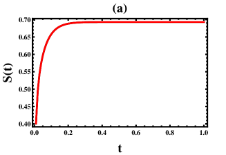
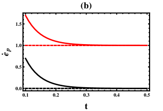
Figure 1: (Color online)(a) The entropy $S(t)$ as a function of $t$ for fixed $f=1$ and $T=1$. $S(t)$ monotonously increases with $t$ and saturates to a constant value as $t$ further increases. (b) The plot ${\dot{e}}_{p}(t)$ (red solid line) and ${\dot{h}}_{d}(t)$ (red dashed line) as a function of $t$ for parameter choice $T=1$. The figure exhibits that in the presence of load ($f=1$), ${\dot{e}}_{p}(t)$ decreases as time increases and in long time limit, it approaches its steady state value ${\dot{e}}_{p}(t)=1$. In the absence of load $f=0$ and for parameter choice of $T=1$, ${\dot{e}}_{p}(t)$ (black solid line) and ${\dot{h}}_{d}(t)$ (black dashed line) monotonously decrease and approach zero.

Since we have an exact analytic expression for $P(x,t)$, let us explore Eq. (11) in detail. As stated before ${\dot{e}}_{p}={\dot{h}}_{d}+{dS(t)\over dt}$ where ${dS(t)\over dt}=-\int{J\over P(x,t)}{\partial\over\partial x}P(x,t)dx$. After some algebra, we write

$${dS(t)\over dt} = \int J{\sum_{n=0}^{\infty}{n\pi\over L}\sin[{n\pi\over L}(x+tf)]e^{-({n\pi\over L})^{2}tT}\over\sum_{n=0}^{\infty}\cos[{n\pi\over L}(x+tf)]e^{-({n\pi\over L})^{2}tT}}dx.$$ (28)

In the limit $t\to\infty$, ${dS(t)\over dt}=0$ since the nominator in Eq. (28) approaches $0$ while the denominator goes to one. This implies that in the long time limit ${\dot{e}}_{p}={\dot{h}}_{d}$ as expected. On the other hand, in the limit $t\to 0$, one can clearly see that ${\dot{e}}_{p}>{\dot{h}}_{d}$.

In this section, let us take the following dimensionless load ${\bar{f}}=fL_{0}/T_{c}$, temperature ${\bar{T}}=T/T_{c}$ where $T_{c}$ is the reference temperature of the isothermal medium. We also introduced dimensionless parameter ${\bar{x}}=x/L_{0}$. For convenience, hereafter the bar will be dropped. From now on all the figures in this section will be plotted in terms of the dimensionless parameters. When $f=0$, the particle freely diffuses without the influence of the external load. Via Eqs. (4), (9) and (10), the dependence of $S(t)$, ${\dot{S}}(t)$, ${\dot{e}}_{p}(t)$ and ${\dot{h}}_{d}(t)$ on model parameters can be explored. In Fig. 1a, $S(t)$ as a function of $t$ is plotted for fixed values of $T=1$ and $f=1.0$. The figure depicts that $S(t)$ monotonously increases with $t$ and saturates to a constant value as $t$ further increases. In the limit $t\to 0$, $S\to 0$ and as $t\to\infty$, $S$ saturates to $S=\ln 2$ confirming the Boltzmann entropy $S=k_{B}\ln\Omega$ where in our case the number of accessible state $\Omega=2$ which agrees with the result shown in the next section. Fig. 1b depicts the plot ${\dot{e}}_{p}(t)$ as a function of $t$ (solid lines). In the same figure, the plot of ${\dot{h}}_{d}(t)$ versus $t$ is shown (dashed line). The figure exhibits that in the presence of load, ${\dot{e}}_{p}(t)$ decreases as time increases and in long time limit, it approaches its steady state value ${\dot{e}}_{p}(t)=1$ (see the red solid line). ${\dot{h}}_{d}(t)$ also approaches its steady state value (see the red dashed line) and at steady state ${\dot{h}}_{d}(t)={\dot{e}}_{p}(t)=1$ showing that at steady state ${\dot{h}}_{d}(t)={\dot{e}}_{p}(t)>0$. This also indicates that in the presence of symmetry breaking fields such as external force, the system is driven out of equilibrium.

The situation is completely different in the absence of external load $f=0$. In this case, ${\dot{e}}_{p}(t)$ monotonously decreases and approaches zero in long time limit (see the black solid line). At stationary state ${\dot{h}}_{d}(t)={\dot{e}}_{p}(t)=0$ revealing that the system approaches its equilibrium state as time progresses. The dependence for the free energy dissipation rate ${\dot{F}}$ as a function time $t$ is explored as depicted in Fig. 2. The figure shows that ${\dot{F}}<0$ and it increases with time and approaches zero.

All of these results qualitatively agree with our previous results mu17 ; muu17 . Furthermore our analysis indicates that $\Delta h_{d}(t)=h_{d}(t)-h_{d}(t_{0})>0$, $\Delta S(t)=S(t)-S(t_{0})>0$ or $\Delta e_{p}(t)=e_{p}(t)-e_{p}(t_{0})>0$ since once the motor starts operating, entropy will be accumulated in the system starting from $t=0$ and as time progresses, more entropy will be stored in the system even though some entropy is extracted out of the system. Hence if the change in these parameters is taken between $t=0$ and any time $t$, always the inequality holds true even for the case $f=0$.

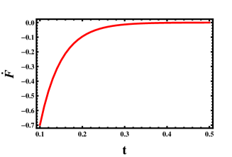
Figure 2: (Color online) ${\dot{F}}$ as a function time $t$ for fixed $T=1$ and $f=0$. The figure shows that ${\dot{F}}<0$ and it increases with time and approaches zero.

III.2 Nonisothermal case

For spatially varying temperature case, let us consider a Brownian particle that freely diffuses (in the absence of load) on one dimensional lattice where the lattices are periodically in contact with the hot $T_{h}$ and cold $T_{c}$ baths. Moreover, the one dimensional lattice has spacing $d$ and in one cycle, the particle walks a net displacement of one lattice site. The jump probability for the particle to hop from site $i$ to $i+1$ is given by $\Gamma e^{-\Delta E/k_{B}T_{i}}$ where $\Delta E=U_{i+1}-U_{i}$ and $\Gamma$ is the probability attempting a jump per unit time mu17 ; muu17 . $k_{B}$ designates the Boltzmann constant and hereafter $\Delta E=0$. $k_{B}$, $\Gamma$ and $d$ are considered to be a unity. The master equation which governs the system dynamics is given by

$${dP_{n}\over dt}=\sum_{n\neq n^{\prime}}\left(P_{nn^{\prime}}p_{n^{\prime}}-P_{n^{\prime}n}p_{n}\right),~{}~{}n,n^{\prime}=1,2,3$$ (29)

where $P_{n^{\prime}n}$ is the transition probability rate at which the system, originally in state $n$, makes transition to state $n^{\prime}$. Here $P_{n^{\prime}n}$ is given by $P_{21}={1\over 2},~{}P_{12}={1\over 2}$. The rate equation for the model can then be expressed as a matrix equation ${d\vec{p}\over dt}={\mathbb{P}}\vec{p}$ where $\vec{p}=(p_{1},p_{2})^{T}$. ${\mathbb{P}}$ is a 2 by 2 matrix which is given by

$${\mathbb{P}}=\left(\begin{array}[]{ccc}-{1\over 2},&~{}{1\over 2}\\ ~{}{1\over 2},&-{1\over 2}\end{array}\right).$$ (30)

Note that the sum of each column of the matrix ${\mathbb{P}}$ is zero, $\sum_{m}{\mathbb{P}}_{mn}=0$ which reveals that the total probability is conserved: $(d/dt)\sum_{n}p_{n}=d/dt({\mathbb{1}}^{T}\cdot p)={\mathbb{1}}^{T}\cdot({\mathbb{P}}\vec{p})=0$.

For the particle which is initially situated at site $i=1$, by solving Eq. (30), we find the time dependent normalized probability distributions for $p_{1}(t)$ and $p_{2}(t)$ as

$$p_{1}(t)={1\over 2}-{e^{-t}\over 2}$$ (31)

and

$$p_{2}(t)={1\over 2}+{e^{-t}\over 2}.$$ (32)

The above equations are dimensionless since $\Gamma$ is considered to be unity.

The velocity of the particle is given by

$$V(t) = p_{1}P_{21}-p_{2}P_{12}$$ (33)

$$= -{e^{-t}\over 2}.$$

The velocity as well as all thermodynamic quantities are not a function of $T_{h}$ and $T_{c}$. In other words, the derived thermodynamic quantities are not different from the isothermal temperature case since the local escape rates are independent of $T_{h}$ and $T_{c}$. This makes sense since for any lattice system (in the absence of external force or potential) which is in contact with a spatially varying temperature should obey the detail balance condition in long time limit. Hence the net velocity is zero as $t$ approach infinity. This also implies that the entropy production as well as the entropy extraction rates become zero in the long time limit; at stationery state the system is reversible. Here care must be taken that in reality the entropy production as well as extraction rate cannot be zero as long as $T_{h}\neq T_{c}$. Here the discrepancy comes from the fact that the Gibbs entropy approach does not take into account the heat exchange due to particle recrossing at the boundary between the hot and cold reservoir. If the heat exchange via kinetic energy is included ${\dot{h}}_{d}(t)\neq 0$ and ${\dot{e}}_{p}(t)\neq 0$ .

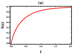
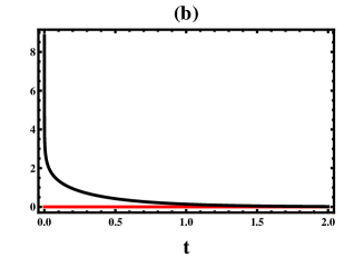
Figure 3: (Color online) (a) The entropy $S(t)$ as a function of $t$ for fixed $\tau=1$. $S(t)$ monotonously increases with $t$ and saturates to a constant value as $t$ further increases. (b) The plot ${\dot{e}}_{p}(t)$ (black solid line) and ${\dot{h}}_{d}(t)$ (red solid line) as a function of $t$ for parameter choice $\tau=1$. The figure exhibits that ${\dot{e}}_{p}(t)$ decreases as time increases and in long time limit, it approaches its stationary value ${\dot{e}}_{p}(t)={\dot{h}}_{d}(t)=0$.

The fundamental entropy balance equation is given by

$${\dot{S}(t)} = {\dot{e}}_{p}(t)-{\dot{h}}_{d}(t)$$ (34)

where $S$ is the Gibbs entropy given by

$$S(t) = -\sum_{i=1}^{2}p_{i}\ln p_{i}$$ (35)

$$= -\left({1\over 2}-{e^{-t}\over 2}\right)\ln{\left({1\over 2}-{e^{-t}\over 2}\right)}-$$

$$\left({1\over 2}+{e^{-t}\over 2}\right)\ln{\left({1\over 2}+{e^{-t}\over 2}\right)}.$$

Exploiting Eq. (35) one can see that in the limit $t\to 0$, $S\to 0$ while in the limit $t\to\infty$, $S\to\ln{2}$. This does make sense, since the system is approaching equilibrium, $S=k_{B}\ln{\Omega}$. Here $k_{B}$ is Boltzmann constant and $\Omega$ is the number of microstates available. In our case $\Omega=2$ since we have only two microstates. Hereafter all figures are plotted by taking dimensionless temperature $\tau={T_{h}\over T_{c}}$ and hereafter the bar will be dropped.

As shown in Fig. 3a, $S$ increases with $t$ and for large $t$, $S$ saturates to constant value similar to Fig. 1a. Next, in terms of the the model parameters, we write ${\dot{h}}_{d}(t)$ and ${\dot{e}}_{p}(t)$ as

$${\dot{h}}_{d}(t) = \sum_{i>j}(p_{i}P_{ji}-p_{j}P_{ij})\ln\left({P_{ji}\over P_{ij}}\right)=0$$ (36)

and

$${\dot{e}}_{p}(t) = \sum_{i>j}(p_{i}P_{ji}-p_{j}P_{ij})\ln\left({p_{i}P_{ji}\over p_{j}P_{ij}}\right)$$ (37)

$$= -(1/2)e^{-t}ln[Tanh[t/2]].$$

From the above analysis one deduces that in the absence of potential, the resulting thermodynamic relations are independent of $T(x)$. Moreover, as depicted in Fig. 3b, ${\dot{h}}_{d}(t)$ is always zero similar to the previous case. ${\dot{e}}_{p}(t)$ decreases with time and as $t$ progresses, it saturates to zero as expected (see Fig. 3b). The total internal energy is also zero.

One should note that since our model system obeys detail balance condition, in long time limit, our system is reversible. However, the energy exchange due to particle recrossing at the boundary between the hot and cold reservoirs is not included. If the heat exchange via kinetic energy is included, our system is irreversible even at a quasistatic limit. This is because even if the particle average velocity is zero, its speed is nonzero. If the particle by chance hops from the cold to hot reservoirs, it absorbs heat and later dumps this heat to the cold bath which indicates that there is always irreversible heat flow from the hot to cold baths and hence the system is always far from equilibrium.

IV Brownian particle walking in a ratchet potential where the potential is coupled with a spatially varying temperature

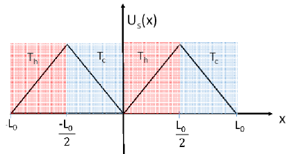
Figure 4: (Color online) Schematic diagram for a Brownian particle in a piecewise linear potential in the absence of external load.

In this section we discuss the non-equilibrium thermodynamics properties of a Brownian particle that walks on the potential $U(x)=U_{s}(x)+fx$ where $f$ and $U_{s}(x)$ denote the load and ratchet potential, respectively am14 . The ratchet potential $U_{s}(x)$

$$U_{s}(x)=\left\{\begin{array}[]{cl}2U_{0}[{x\over L}],&if~{}0<x\leq L/2;\\ 2U_{0}[{-x\over L}+1],&if~{}L/2<x\leq L;\end{array}\right.$$ (38)

is coupled along the reaction coordinate in the manner

$$T(x)=\left\{\begin{array}[]{ll}T_{h},&\text{if}~{}~{}~{}0\leq x\leq{L_{0}\over 2};\\ T_{c},&\text{if}~{}~{}~{}{L_{0}\over 2}\leq x\leq L_{0}.\end{array}\right.$$ (39)

The parameters $U_{0}$ and $L$ denote the barrier height and the width of the ratchet potential, respectively. The ratchet potential has a potential maxima at $x=L/2$ and potential minima at $x=0$ and $x=L$. The potential profile repeats itself such that $U_{s}(x+L)=U_{s}(x)$. In the high friction limit, the dynamics of the particle is governed by the Langevin equation (1). In this section, let us take the following dimensionless load ${\bar{f}}=fL_{0}/T_{c}$, temperature ${\bar{T}}(x)=T(x)/T_{c}$, barrier height ${\bar{U}_{0}}=U_{0}/T_{c}$ and length ${\bar{x}}=x/L_{0}$. We also introduced dimensionless parameters $\tau=T_{h}/T_{c}$ and $\beta=\gamma(x)L_{0}^{2}/T_{c}$. From now on all the figures in this section will be plotted in terms of the dimensionless parameters and hereafter we drop all the bars and take $\beta$ to be unity. Next we discuss the short time behavior of the system via numerical simulations.

IV.1 Short time case

As discussed in many litterateurs, for a Brownian particle walking in a ratchet potential, the system attains a unidirectional motion as long as a distinct temperature difference is retained between the hot and cold baths. For isothermal case the particle undergoes a random walk with average zero velocity, see Fig. 5a. One can also see the probability of finding the particle is higher in the vicinity the two potential minima (see Fig. 5b). As time progresses, the probability of finding the particle in the vicinity of the potential minima decreases which implies that the entropy of the system increases as time progresses. One can note that for isothermal case, if the system reaches stationary state and if the change in these parameters are taken at this particular state, then $\Delta h_{d}=0$, $\Delta S=0$ or $\Delta e_{p}=0$. In reality, when the particle relaxes to its equilibrium state, it produces entropy and once the motor starts operating, entropy will be accumulated in the system starting from $t=0$ and as time progresses, more entropy will be stored in the system even though some entropy is extracted out of the system. Hence if the change in these parameters is taken between $t=0$ and any time $t$, always the inequality $\Delta h_{d}(t)=h_{d}(t)-h_{d}(0)>0$, $\Delta S(t)=S(t)-S(0)>0$ or $\Delta e_{p}(t)=e_{p}(t)-e_{p}(0)>0$ holds true and as time progresses the change in this parameters increases. In fact, in small $t$ regimes, ${\dot{e}}_{p}(t)$ becomes much larger than ${\dot{h}}_{d}(t)$ revealing that the entropy production is higher (than entropy extraction) in the first few period of times. As time increases, more entropy will be extracted ${\dot{h}}_{d}(t)>{\dot{e}}_{p}$. Over all, since the system produces enormous amount of entropy at initial time, in latter time or any time $t$, $\Delta e_{p}(t)>\Delta h_{d}(t)$ and hence $\Delta S(t)>0$.

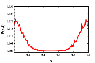
Figure 5: (Color online)(a) Trajectory $x$ as a function time $t$ for fixed $f=0.0$ is evaluated via numerical simulations. Other parameters are fixed as $U_{0}=4$, $\tau=1.0$. (b) The probability $P(x,t)$ as a function time $t$ for fixed $f=0.0$, $U_{0}=4$ and $\tau=1.0$

On the other hand, when a distinct temperature difference between the hot and cold reservoirs is retained, the particle attains a non-zero velocity. Its trajectory also indicates that the particle undergoes a biased random walk (see Figs. 6a) with high probability to reside in one of the potential well (see Fig. 6b) at small time $t$. As time gets increased, the probability of finding the particle near the potential wells decreases and at steady state the probability approaches its steady state value. The particles current or equivalently the velocity also increases as time increases and as time further gets increased, it approaches its exact steady state value (Eq. (41)).

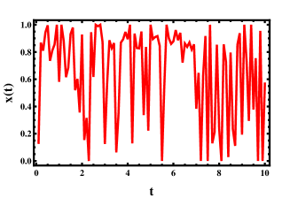
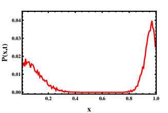
Figure 6: (Color online)(a) Trajectory $x$ as a function time $t$ for given $f=0.0$, $U_{0}=4$ and $\tau=4.0$. (b) The probability $P(x,t)$ as a function time $t$ for a given values of $f=0.0$, $U_{0}=8.0$ and $\tau=4.0$.

Next via numerical simulations, we study how the entropy of the system behaves as time varies. The entropy of the system exhibits an intriguing parameter dependence. In Fig. 7, we plot the entropy $S$ as a function of $t$ for parameter choice of $U_{0}=4.0$, $\tau=4$, $\lambda=0$. The figure once again shows that the entropy increases as time steps up. As time further increases, the entropy saturates to a constant value which qualitatively agrees the result shown in the previous sections.

Figure 7: (Color online) The entropy $S(t)$ as a function time $t$ a given values of $f=0.0$, $U_{0}=8.0$, $\tau=8.0$. As time progresses, the entropy saturates to constant value.

Let us focus on the rate of entropy production ${\dot{e}}_{p}(t)$ and the rate of entropy flow from the system to the outside ${\dot{h}}_{d}(t)$. The plot of ${\dot{e}}_{p}(t)$ (dashed red line) and ${\dot{h}}_{d}(t)$ (solid black line) as a function of $t$ is depicted in Figs. 8a and 8b, respectively for fixed values of $U_{0}=4.0$, $\tau=2.0$ and $\lambda=0$. The figures indicate that far from steady state ${\dot{e}}_{p}(t)>0$ and ${\dot{h}}_{d}(t)>0$. When $t\to 0$, ${\dot{e}}_{p}(t)$ becomes much greater than ${\dot{h}}_{d}(t)$ and as time progresses ${\dot{e}}_{p}(t)$ and ${\dot{h}}_{d}(t)$ decrease and approach their steady state value. At steady state, ${\dot{e}}_{p}={\dot{h}}_{d}>0$. All these results qualitatively agree with the results which are shown in previous section as well as the results reported in the works mu17 ; muu17 .

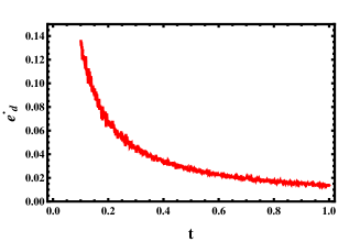
Figure 8: (Color online)(a) ${\dot{e}}_{p}(t)$ as a function of $t$ for fixed $f=0.0$, $U_{0}=8.0$, $\tau=8.0$. (b) The plot for ${\dot{h}}_{p}(t)$ as a function of $t$ for fixed $f=0.0$, $U_{0}=8.0$, $\tau=8.0$.

IV.2 Long time case

Let us now focus on the long time behavior of the system. In this limit, the closed form expression for the steady state current am14 is given by

$$J=-{\varsigma_{1}\over\varsigma_{2}\varsigma_{3}+\varsigma_{4}\varsigma_{1}}$$ (40)

where the expressions for $\varsigma_{1}$, $\varsigma_{2}$, $\varsigma_{3}$ and $\varsigma_{4}$ are given as $\varsigma_{1}=e^{a-b}-1$, $\varsigma_{2}={\over a\tau}\left(1-e^{-a}\right)+{\over b}e^{-a}\left(e^{b}-1\right)$, $\varsigma_{3}={1\over a}\left(e^{a}-1\right)+{1\over b}e^{a}\left(1-e^{-b}\right)$. The parameter $\varsigma_{4}$ is given by $\varsigma_{4}=\epsilon_{1}+\epsilon_{2}+\epsilon_{3}$ where $\epsilon_{1}={1\over\tau}\left({1\over a}\right)^{2}\left(a+e^{-a}-1\right)$, $\epsilon_{2}={1\over ab}\left(1-e^{-a}\right)\left(e^{b}-1\right)$, $\epsilon_{3}=\left({1\over b}\right)^{2}\left(e^{b}-1-b\right)$. Here $a=\left(U_{0}+f\right)/\tau$ and $b=\left(U_{0}-f\right)$.

Before we explore the dependence of the thermodynamic quantities on the model parameters, let us first compute the expressions for the useful work and the heat input. Via the stochastic approach, one finds

$${\dot{W}}^{L}=fLJ$$ (41)

and in order to do this useful work the particle should get a minimum input energy

$${\dot{Q}}_{h}=U_{0}J+fJL/2$$ (42)

from the hotter region. The heat dissipated to the colder region is then given by

$${\dot{Q}}_{c}=U_{0}J-fJL/2.$$ (43)

Since the term $T^{\prime}(x)$ vanishes when a periodic boundary condition is imposed, ${\dot{W}}^{T}=0$. The second law of thermodynamics can be rewritten in terms of the housekeeping heat and excess heat. For the model system we consider, when the particle undergoes a cyclic motion, at least it has to get $fLJ$ amount of energy rate from the hot reservoir in order to keep the system at steady state. Hence $fLJ$ is equivalent to the housekeeping heat $Q_{hk}$ and we can rewrite Eq. (20) as

$${\dot{F}}(t)+{\dot{E}}_{p}(t)={\dot{E}}_{in}(t)+{\dot{H}}_{d}(t)=-fLJ=-{\dot{Q}}_{hk}$$ (44)

while the expression for the excess heat ${\dot{Q}}_{ex}$ is given by

$$Q_{ex}={\dot{H}}_{d}-{\dot{Q}}_{hk}.$$ (45)

For isothermal case ($\tau=1$), we can rewrite the second law of thermodynamics as

$${\dot{S}}^{T}(t)={\dot{E}}_{p}-{\dot{H}}_{d}={-\dot{F}}-{\dot{Q}}_{ex}$$ (46)

and

$${\dot{F}}={\dot{Q}}_{hk}-{\dot{E}}_{p}.$$ (47)

Figure 9: (Color online)(a) $J$ as a function of $U_{0}$ for fixed $\tau=2$, $f=0.2$, $f=0.4$ and $f=0.6$, from top to bottom. (b) The plot for $J$ as a function of $f$ for fixed $\tau=2$, $U_{0}=1$, $U_{0}=2$ and $U_{0}=4$ from top to bottom.

Next, via Eq. (40), let us explore the dependence of the particle current on model parameters. The current $J$ as a function of $U_{0}$ is plotted in Fig. 9a. The figure depicts that the current increases as $U_{0}$ increases. At stall force $J=0$. As $U_{0}$ further increases, the current attains an optimal value and at this particular parameter of space, the motor moves fast at the expense of high energy expenditure. On the other hand, the plot $J$ as a function of $f$ depicts that the current decreases as the load increases (see Fig. 9b). At stall force

$$f_{s}={2(\tau-1)U_{0}\over(\tau+1)}$$ (48)

the current vanishes $J=0$. $f_{s}$ shifts to the left as $U_{0}$ increases.

Figure 10: (Color online)(a) ${\dot{e}}_{p}(t)$ as a function of $U_{0}$ for fixed $f=0.2$, $f=0.4$ and $f=0.6$, from top to bottom. (b) The plot for ${\dot{e}}_{p}(t)$ as a function of $f$ for fixed $U_{0}=1$, $U_{0}=2$ and $U_{0}=4$ from top to bottom.

At steady state, ${\dot{e}}_{p}(t)={\dot{h}}_{d}(t)$. Using the steady stated current derived in this work as well as via Eqs. (9) and (10), let us now evaluate how ${\dot{e}}_{p}(t)$ or ${\dot{h}}_{d}(t)$ behaves. In Fig. 10a, we plot ${\dot{e}}_{p}(t)$ as a function of $U_{0}$ for fixed $f=0.2$, $f=0.4$ and $f=0.6$, from top to bottom. The figure depicts that ${\dot{e}}_{p}(t)$ decreases as $U_{0}$ increases and it vanishes at certain potential $U_{0}^{s}$ which clearly exhibits that at quasistatic limit $U_{0}\to U_{0}^{s}$, ${\dot{e}}_{p}(t)=0$. As $U_{0}$ increases, ${\dot{e}}_{p}(t)$ increases and peaks at particular $U_{0}$. This makes sense since at this particular choice of parameter, the system operates at maximum power. As $U_{0}$ further increases, ${\dot{e}}_{p}(t)$ steps down. In Figure 10b, ${\dot{e}}_{p}(t)$ as a function of the load $f$ is plotted for fixed $U_{0}=1$, $U_{0}=2$ and $U_{0}=4$ from bottom to top. ${\dot{e}}_{p}(t)$ decreases as $f$ increases and at stall force ${\dot{e}}_{p}(t)=0$. As the load further increases, ${\dot{e}}_{p}(t)$ steps up.

Figure 11: (Color online) Phase space for $f$ as a function time $\tau$ for fixed $f=0.2$. Other parameters are fixed as $U_{0}=1$, $U_{0}=2$ and $U_{0}=4$ from bottom to top.

The phase space at which the system is reversible is also depicted in parameter space of the load $f$ and $\tau$ in Fig. 12 for fixed $f=0.2$. Other parameters are fixed as $U_{0}=1$, $U_{0}=2$ and $U_{0}=4$ from bottom to top.

V Summary and conclusion

In this work, the general expressions for the free energy, entropy production and entropy extraction rates are derived for a Brownian particle moving in a viscous medium where the dynamics of its motion is governed by the Langevin equation. Via Boltzmann-Gibbs nonequilibrium entropy as well as from the knowledge of local probability density and particle current, several thermodynamic relations are derived. Far from equilibrium, we show that the system constantly produces entropy and at the same time extracts entropy out of the system. The entropy production and extraction rates decrease in time and saturate to a constant value. The rate of entropy production balances the rate of entropy extraction as long as the system is at steady state while at equilibrium both entropy production and extraction rates become zero.

We further consider different model systems and explore how their thermodynamic features such as the free energy, entropy production and entropy extraction rates behave as a function of the model parameters. For Brownian particle that hops on a periodic isothermal medium (in the presence or absence of load), it is shown that the entropy $S(t)$ monotonously increases with time and saturates to a constant value as $t$ further steps up. The entropy production rate ${\dot{e}}_{p}$ decreases in time and at steady state (in the presence of load), ${\dot{e}}_{p}={\dot{h}}_{d}>0$. At stationary state (in the absence of load), ${\dot{e}}_{p}={\dot{h}}_{d}=0$. On the contrary, when the particle hops on nonisothermal medium, we show that the derived thermodynamic quantities are not different from the isothermal temperature case as long as the external load is zero. Furthermore, we discuss the thermodynamics features of a Brownian particle that hops in a ratchet potential where the potential is coupled with a spatially temperature. It is shown that the operational regime of such Brownian heat engine is dictated by the magnitude of the external load $f$. The particle current or equivalently the velocity of the engine is positive when $f$ is smaller and the engine acts as a heat engine. In this regime ${\dot{e}}_{p}={\dot{h}}_{d}>0$. When $f$ increases, the velocity of the particle decreases and at stall force, we find that ${\dot{e}}_{p}={\dot{h}}_{d}=0$ showing that the system is revertible at this particular choice of parameter. For large load, the current is negative and the engine acts as a refrigerator. In this region ${\dot{e}}_{p}={\dot{h}}_{d}>0$.

In conclusion, in this work we present a simple model that serves a starting point to study the thermodynamics features many practical problems such as intracellular transport of kinesin or dynein which can be modeled as particles walking on lattice; see for example the works by T. Bameta $et$. $al$. mu28 , D. Oriola $et$. $al$. mu29 and O. Camp s $et$. $al$. mu30 . The present model also serves as a tool to check many elegant thermodynamic theories. Based on this exactly solvable models, we expose several thermodynamic relations. We believe that the result obtained in this work is generic and advances the nonequilibruim thermodynamics.

References

- (1) H. Ge and H. Qian, Phys. Rev. E 81, 051133 (2010).
- (2) T. Tome and M. J. de Oliveira, Phys. Rev. Lett. 108, 020601 (2012).
- (3) J. Schnakenberg, Rev. Mod. Phys. 48, 571 (1976).
- (4) T. Tome and M.J. de Oliveira, Phys. Rev. E 82, 021120 (2010).
- (5) R.K.P. Zia and B. Schmittmann, J. Stat. Mech. P07012 (2007).
- (6) U. Seifert, Phys. Rev. Lett. 95, 040602 (2005).
- (7) T. Tome, Braz. J. Phys. 36, 1285 (2006).
- (8) G. Szabo, T. Tome and I. Borsos, Phys. Rev. E 82, 011105 (2010).
- (9) B. Gaveau, M. Moreau and L.S. Schulman, Phys. Rev. E 79, 010102 (2009).
- (10) J.L. Lebowitz and H. Spohn, J. Stat. Phys. 95, 333 (1999).
- (11) D. Andrieux and P. Gaspar, J. Stat. Phys. 127, 107 (2007).
- (12) R.J. Harris and G.M. Schutz, J. Stat. Mech. P07020 (2007).
- (13) J.-L. Luo, C. Van den Broeck, and G. Nicolis, Z. Phys. B 56, 165 (1984).
- (14) C.Y. Mou, J.-L. Luo, and G. Nicolis, J. Chem. Phys. 84, 7011 (1986).
- (15) C. Maes and K. Netocny, J. Stat. Phys. 110, 269 (2003).
- (16) L. Crochik and T. Tome, Phys. Rev. E 72, 057103 (2005).
- (17) M. Asfaw, Phys. Rev. E 89, 012143 (2014).
- (18) M. Asfaw, Phys. Rev. E 92, 032126 (2015).
- (19) K. Brandner, M. Bauer, M. Schmid and U. Seifert, New. J. Phys. 17, 065006 (2015).
- (20) B. Gaveau, M. Moreau and L. S. Schulman, Phys. Rev. E 82, 051109 (2010).
- (21) E. Boukobza and D.J. Tannor, Phys. Rev. Lett. 98, 240601 (2007).
- (22) T. Bameta, D. Das, R. Padinhateeri and M. M. Inamdar, ArXiv:1503.06529 (2015).
- (23) D. Oriola and J. Casademunt, Phys. Rev. Lett. 111, 048103 (2013).
- (24) O. Campa, Y. Kafri, K.B. Zeldovich, J. Casademunt and J.-F. Joanny, Phys. Rev. Lett. 97, 038101 (2006).
- (25) P. Hänggi, Helv. Phys. Acta 51, 183 (1978).
- (26) P. Hänggi, Helv. Phys. Acta 53, 491 (1980).
- (27) J. M. Sancho, M. S. Miguel and D. Duerr, J. Stat. Phys. 28, 291 (1982).
- (28) K. Sekimoto, J. Phys. Soc. Jpn. 66, 1234 (1997).
- (29) K. Sekimoto, Prog. Theor. Phys. Suppl. 130, 17 (1998).
- (30) T. Hondou and K. Sekimoto, Phys. Rev. E 62, 6021 (2000).
- (31) Y. Oono and M. Paniconi, Prog. Theor. Phys. 130, 29 (1998).
- (32) J. Parrondo, B. Jimenez de Cisneros and R. Brito, Stochastic Processes in Physics, Chemistry and Biology LNP557 (Springer-Verlag, Berlin (2000)), p. 38.
- (33) S. Lahiri, S. Rana, and A. M. Jayannavar, Phys. Letters A, 378, 979 (2014).
- (34) M. Asfaw, Eur. Phys. J. B 86, 189 (2014).