Prior-Based Model Checking

Abstract

Model checking procedures are considered based on the use of the Dirichlet process and relative belief. This combination is seen to lead to some unique advantages for this problem. In particular, it avoids double use of the data and prior-data conflict. Several examples have been incorporated, in which the proposed approach exhibits excellent performance.

1 Introduction

This paper is concerned with checking whether or not a chosen statistical model $\{P_{\theta}:\theta\in\Theta\}$ is in agreement with observed data $x\in\mathfrak{X},$ where $\mathfrak{X}$ is the sample space with $\sigma$-algebra $\mathcal{A}$ and each $P_{\theta}$ is a probability measure on $\mathcal{A}.$ If it is determined that the observed data does not contradict the model, then inferences can proceed about the true value of $\theta\in\Theta$. If the model fails to pass its checks, then there is a concern about the correctness of the inferences. Thus, checking a proposed model based on the observed data is a matter of some significance.

While there have been many methods developed for model checking, the approach taken here is Bayesian in nature in that a prior is placed on the set of all probability measures on $(\mathfrak{X},\mathcal{A)}$ and inference is then conducted concerning model correctness. The approach taken to inference is based on a particular measure of evidence known as the relative belief ratio which measures how beliefs have changed from a priori to a posteriori. So a relative belief ratio is computed which indicates whether there is evidence for or against the model $\{P_{\theta}:\theta\in\Theta\}$ holding. Furthermore, a calibration of this evidence is provided concerning whether there is strong or weak evidence for or against the model. Relative belief ratios and the associated inferences are discussed in Section 2.

Recently, there has been considerable interest in developing Bayesian nonparametric procedures for model checking. Most of this has focused on embedding the proposed model as a null hypothesis in a larger family of distributions. Then priors are placed on the null and the alternative and a Bayes factor is computed. For example, Florens, Richard, and Rolin (1996) used a Dirichlet process for the prior on the alternative. Carota and Parmigiani (1996), Verdinelli and Wasserman (1998), Berger and Guglielmi (2001) and McVinish, Rousseau, and Mengersen (2009) considered a mixture of Dirichlet processes, a mixture of Gaussian processes, a mixture of Pólya trees and a mixture of triangular distributions, respectively, for the prior on the alternative. Another approach for model testing is based on placing a prior on the true distribution generating the data and measuring the distance between the posterior distribution and the proposed one. Swartz (1999) and Al-Labadi and Zarepour (2013, 2014) considered the Dirichlet process prior and used the Kolmogorov distance to derive a goodness-of-fit test for continuous models. Viele (2000) used the Dirichlet process and the Kullback-Leibler distance to test only discrete models. Hsieh (2011) used the Pólya tree prior and the Kullback-Leibler distance to test continuous distributions.

The methodology developed in this paper combines the previous two approaches and provides some unique, beneficial features. A Dirichlet process $DP(a,H)$ is considered as a prior on the set of all distributions on $(\mathfrak{X},\mathcal{A)}$ and then the concentration of the posterior distribution about the model of interest is compared to the concentration of the prior distribution about the model of interest. This comparison is made via a relative belief ratio to measure the evidence in the observed data for or against the model. A measure of the strength of this evidence is also provided. Implementing the approach is fairly simple and does not require obtaining a closed form of the relative belief ratio. The methodology does not require the use of a prior on $\theta$ and so is truly a check on the model itself avoiding any issues with the prior on $\theta.$ It is shown that, by appropriate choices of the hyperparameters $a$ and $H,$ prior-data conflict with respect to $DP(a,H),$ namely, the distributions in the model lie in the tails of the prior, can be avoided. Any prior on $\theta$ should be checked for prior-data conflict separately from a check on the model, and only when the model passes its checks, as this avoids confounding model error with error introduced by a poor choice of a prior, see Evans and Moshonov (2006).

In Section 3 the Dirichlet process prior $DP(a,H)$ is briefly reviewed and in Section 4 the basis of our goodness-of-fit measure, namely, the Cramér-von Mises distance between probability measures is discussed. Section 5 deals with the heart of our proposal where it is argued that a particular usage of the Cramér-von Mises distance together with particular choices of the hyperparameters $(a,H)$ be employed. In Section 6 a computational algorithm is developed for the implementation of relative belief inferences in this context. Section 7 presents a number of examples where the behavior of the methodology is examined in some detail.

2 Relative Belief Ratios

Let $\{f_{\theta}:\theta\in\Theta\}$ denote a collection of densities on a sample space $\mathcal{X}$ and let $\pi$ denote a prior on $\Theta.$ After observing data $x,$ the posterior distribution of $\theta$ is given by the density $\pi(\theta\,|\,x)=\pi(\theta)f_{\theta}(x)/m(x)$ where $m(x)=\int_{\Theta}\pi(\theta)f_{\theta}(x)\,d\theta$ is the prior predictive density of $x.$ For an arbitrary parameter of interest $\psi=\Psi(\theta),$ denote the prior and posterior densities of $\psi$ by $\pi_{\Psi}$ and $\pi_{\Psi}(\cdot\,|\,x),$ respectively. The relative belief ratio for a value $\psi$ is then defined by $RB_{\Psi}(\psi\,|\,x)=\lim_{\delta\rightarrow 0}\Pi_{\Psi}(N_{\delta}(\psi\,)|\,x)/\Pi_{\Psi}(N_{\delta}(\psi\,)$ where $N_{\delta}(\psi\,)$ is a sequence of neighborhoods of $\psi$ converging (nicely) to $\psi$ as $\delta\rightarrow 0.$ Quite generally

$$RB_{\Psi}(\psi\,|\,x)=\pi_{\Psi}(\psi\,|\,x)/\pi_{\Psi}(\psi),$$ (1)

the ratio of the posterior density to the prior density at $\psi.$ So $RB_{\Psi}(\psi\,|\,x)$ is measuring how beliefs have changed concerning $\psi$ being the true value from a priori to a posteriori by comparing a posterior probability to a prior probability. Note that a relative belief ratio is similar to a Bayes factor, as both are measures of evidence, but the latter measures this via the change in an odds ratio. The full relationship between relative belief ratios and Bayes factors is discussed in Evans (2015). Our developments here are based on the relative belief ratio as the associated theory is much simpler.

By a basic principle of evidence, when $RB_{\Psi}(\psi\,|\,x)>1$ the data have lead to an increase in the probability that $\psi$ is correct, and so there is evidence in favor of $\psi,$ when $RB_{\Psi}(\psi\,|\,x)<1$ the data have lead to a decrease in the probability that $\psi$ is correct, and so there is evidence against $\psi,$ and when $RB_{\Psi}(\psi\,|\,x)=1$ there is no evidence either way. Note that $RB_{\Psi}(\psi\,|\,x)$ is invariant under smooth changes of variable and also invariant to the choice of the support measure for the densities. As such all relative belief inferences possess this invariance which is not the case for many Bayesian inferences such as using a posterior mode or expectation for estimation.

The value $RB_{\Psi}(\psi_{0}\,|\,x)$ then measures the evidence for the hypothesis $\mathcal{H}_{0}=\{\theta:\Psi(\theta)=\psi_{0}\}.$ It is also necessary, however, to calibrate whether this is strong or weak evidence for or against $\mathcal{H}_{0}.$ Certainly the bigger $RB_{\Psi}(\psi_{0}\,|\,x)$ is than 1, the more evidence there is in favor of $\psi_{0}$ while the smaller $RB_{\Psi}(\psi_{0}\,|\,x)$ is than 1, the more evidence there is against $\psi_{0}.$ But what exactly does a value of $RB_{\Psi}(\psi_{0}\,|\,x)=20$ mean? It would appear to be strong evidence in favor of $\psi_{0}$ because beliefs have increased by a factor of 20 after seeing the data. But what if other values of $\psi$ had even larger increases? A useful calibration of $RB_{\Psi}(\psi_{0}\,|\,x)$ is given by

$$\Pi_{\Psi}(RB_{\Psi}(\psi\,|\,x)\leq RB_{\Psi}(\psi_{0}\,|\,x)\,|\,x),$$ (2)

namely, the posterior probability that the true value of $\psi$ has a relative belief ratio no greater than that of the hypothesized value $\psi_{0}.$ Note that (2) is not a p-value as it has a very different interpretation. When $RB_{\Psi}(\psi_{0}\,|\,x)<1,$ so there is evidence against $\psi_{0},$ then a small value for (2) indicates a large posterior probability that the true value has a relative belief ratio greater than $RB_{\Psi}(\psi_{0}\,|\,x)$ and so there is strong evidence against $\psi_{0}.$ When $RB_{\Psi}(\psi_{0}\,|\,x)>1,$ so there is evidence in favor of $\psi_{0},$ then a large value for (2) indicates a small posterior probability that the true value has a relative belief ratio greater than $RB_{\Psi}(\psi_{0}\,|\,x))$ and so there is strong evidence in favor of $\psi_{0},$ while a small value of (2) only indicates weak evidence in favor of $\psi_{0}.$

As $RB_{\Psi}(\psi\,|\,x)$ measures the evidence that $\psi$ is the true value, it naturally leads to an estimate of $\psi.$ For example, the best estimate of $\psi$ is clearly the value for which the evidence is greatest, namely, $\psi(x)=\arg\sup RB_{\Psi}(\psi\,|\,x).$ Associated with this is a $\gamma$-credible region $C_{\Psi,\gamma}(x)=\{\psi:RB_{\Psi}(\psi\,|\,x)\geq c_{\Psi,\gamma}(x)\}$ where $c_{\Psi,\gamma}(x)=\inf\{k:\Pi_{\Psi}(RB_{\Psi}(\psi\,|\,x)>k\,|\,x)\leq\gamma\}.$ Notice that $\psi(x)\in C_{\Psi,\gamma}(x)$ for every $\gamma\in[0,1]$ and so, for selected $\gamma,$ we can take the ”size” of $C_{\Psi,\gamma}(x)$ as a measure of the accuracy of the estimate $\psi(x).$ The interpretation of $RB_{\Psi}(\psi\,|\,x)$ as the evidence for $\psi\$forces the sets $C_{\Psi,\gamma}(x)$ to be the credible regions. For if $\psi_{1}$ is in such a region and $RB_{\Psi}(\psi_{2}\,|\,x)\geq RB_{\Psi}(\psi_{1}\,|\,x),$ then $\psi_{2}$ must also be in the region as there is at least as much evidence for $\psi_{2}$ as for $\psi_{1}.$

A number of optimality results have been established for relative belief inferences and these are discussed in Evans (2015). For example, suppose we use the relative belief ratio to accept $\mathcal{H}_{0}:\Psi(\theta)=\psi_{0}$ when $RB_{\Psi}(\psi_{0}\,|\,x)>1$ and reject when $RB_{\Psi}(\psi_{0}\,|\,x)<1.$ It is the case then that the acceptance region $A(\psi_{0})=\{x:RB_{\Psi}(\psi_{0}\,|\,x)>1\}$ and the rejection region $R(\psi_{0})=\{x:RB_{\Psi}(\psi_{0}\,|\,x)<1\}$ are optimal among all such regions in the following sense. Let $A\subset\mathcal{X}$ be another acceptance region such that $M(A\,|\,\psi_{0})\geq M(A(\psi_{0})\,|\,\psi_{0})$ where $M(\cdot\,|\,\psi_{0})$ is the conditional prior predictive probability measure given that $\Psi(\theta)=\psi_{0}.$ Then among all such acceptance regions, $A(\psi_{0})$ minimizes the prior probability of rejecting $H_{0}$ when it is false. A similar result holds for $R(\psi_{0}).$ Furthermore, under mild conditions it is proved in Evans (2015) that $M(A(\psi_{0})\,|\,\psi_{0})\rightarrow 1$ and $M(R(\psi_{0})\,|\,\psi_{0})\rightarrow 0$ as the amount of data increases. So the values of $M(A(\psi_{0})\,|\,\psi_{0})$ and $M(R(\psi_{0})\,|\,\psi_{0})$ can be set by design and it is then known that we are using the optimal tests with these characteristics. Numerous additional optimality results are proved for the relative credible regions $C_{\Psi,\gamma}(x)$ and the estimator $\psi(x)$ in Evans (2015).

The view is taken here that anytime continuous probability is used, then this is an approximation to a finite, discrete context. For example, if $\psi$ is a mean and the response measurements are to the nearest centimeter, then of course the true value of $\psi$ cannot be known to an accuracy greater than 1/2 of a centimeter, no matter how large a sample we take. Furthermore, there are implicit bounds associated with any measurement process. As such the restriction is made here to discretized parameters that take only finitely many values. So when $\psi$ is a continuous, real-valued parameter, it is discretized to the intervals $\ldots,(\psi_{0}-3\delta,\psi_{0}-\delta],(\psi_{0}-\delta,\psi_{0}+\delta],(\psi_{0}+\delta,\psi_{0}+3\delta],\ldots$ for some choice of $\delta>0,$ and there are only finitely may such intervals covering the range of possible values. It is of course possible to allow the intervals to vary in length as well. With this discretization, then $H_{0}=$ $(\psi_{0}-\delta,\psi_{0}+\delta].$

Note that throughout the paper the notation $P$ could refer to either a probability measure or its corresponding cdf where the context determines the appropriate interpretation.

3 Dirichlet Process

The Dirichlet process, formally introduced in Ferguson (1973), is the most well-known and widely used prior in Bayesian nonparametric inference. Consider a space $\mathfrak{X}$ with a $\sigma-$algebra $\mathcal{A}$ of subsets of $\mathfrak{X}$. Let $H$ be a fixed probability measure on $(\mathfrak{X},\mathcal{A})$ and $a$ be a positive number. Following Ferguson (1973), a random probability measure $P=\left\{P(A)\right\}_{A\in\mathcal{A}}$ is called a Dirichlet process on $(\mathfrak{X},\mathcal{A})$ with parameters $a$ and $H$, if for any finite measurable partition $\{A_{1},\ldots,A_{k}\}$ of $\mathfrak{X}$, the joint distribution of the vector $\left(P(A_{1}),\ldots\,P(A_{k})\right)$ has the Dirichlet distribution with parameters $(aH(A_{1}),\ldots,$ $aH(A_{k})),$ where $k\geq 2$. We assume that if $H(A_{j})=0$, then $P(A_{j})=0$ with a probability one. If $P$ is a Dirichlet process with parameters $a$ and $H,$ we write $P\sim{DP}(a,H).$ For any $A\in\mathcal{A},$ $P(A)$ has a beta distribution with parameters $aH(A)$ and $a(1-H(A))$ and so ${E}(P(A))=H(A)\ \$ and ${Var}(P(A))=H(A)(1-H(A))/(1+a).$ The probability measure $H$ is called the base measure of $P$. Clearly $H$ plays the role of the center of the process, while $a$ can be viewed as the concentration parameter. The larger $a$ is, the more likely it is that the realization of $P$ is close to $H$.

An attractive feature of the Dirichlet process is the conjugacy property. If $x=(x_{1},\ldots,x_{n})$ is a sample from $P\sim DP(a,H)$, then the posterior distribution of $P$ is $P\,|\,x\sim DP(a+n,H_{x})$ where

$$H_{x}=a(a+n)^{-1}H+n(a+n)^{-1}F_{n},$$ (3)

with $F_{n}=n^{-1}\sum_{i=1}^{n}\delta_{{x}_{i}}$ and $\delta_{x_{i}}$ the Dirac measure at $x_{i}.$ Notice that, the posterior base distribution $H_{x}$ is a convex combination of the prior base distribution and the empirical distribution. The posterior base $H_{x}$ approaches the prior base $H$ as $a\rightarrow\infty$ while $H_{x}$ converges to the empirical distribution as $a\rightarrow 0.$

Ferguson (1973) provided a series representation for $P\sim{DP}(a,H).$ Specifically, let $(E_{k})_{k\geq 1}$ be i.i.d. exponential$(1)$ random variables, $\Gamma_{i}=E_{1}+\cdots+E_{i},(Y_{i})_{i\geq 1}$ be i.i.d. $H$ random variables independent of $(\Gamma_{i})_{i\geq 1}$ and put

$$P=\sum_{i=1}^{\infty}L^{-1}(\Gamma_{i}){\delta_{Y_{i}}/}\sum_{i=1}^{\infty}{{L^{-1}(\Gamma_{i})}},$$ (4)

where $L(x)=a\int_{x}^{\infty}t^{-1}e^{-t}dt,x>0,$ and $L^{-1}(y)=\inf\{x>0:L(x)\geq y\}.$ From (4), it follows clearly that a realization of the Dirichlet process is a discrete probability measure. This is true even when the base measure is absolutely continuous. Note that, although the Dirichlet process is discrete with probability one, this discreteness is no more troublesome than the discreteness of the empirical process. By imposing the weak topology, the support for the Dirichlet process is quite large. Specifically, the support for the Dirichlet process is the set of all probability measures whose support is contained in the support of the base measure. This means if the support of the base measure is $\mathfrak{X}$, then the space of all probability measures is the support of the Dirichlet process. For example, if we have a normal base measure, then the Dirichlet process can choose any probability measure.

Recently, Zarepour and Al-Labadi (2012) derived an efficient series approximation with monotonically decreasing weights for the Dirichlet process . Let $(Y_{i})_{1\leq i\leq N}$ be i.i.d. $H$ independent of $(\Gamma_{i})_{1\leq i\leq{N+1}},G_{a/N}$ be the co-cdf of the g$\text{amma}(a/N,1)$ distribution, and $J_{i}={G_{a/N}^{-1}(\Gamma_{i}/\Gamma_{N+1})/}\sum_{j=1}^{N}{G_{a/N}^{-1}(\Gamma_{j}/\Gamma_{N+1}),}$ then

$$P_{N}=\sum_{i=1}^{N}J_{i}\delta_{Y_{i}}$$ (5)

converges almost surely to $P$ defined by (4), as $N\rightarrow\infty$. Note that ${G_{a/N}^{-1}(p)}$ is the $(1-p)$-th quantile of the g$\text{amma}(\alpha/N,1)$ distribution. This provides the following algorithm.

Algorithm A: Approximately generating a value from $DP(a,H)$

1. Fix a relatively large positive integer $N$.

2. Generate i.i.d. $Y_{i}\sim H$ for $i=1,\ldots,N.$

3. For $i=1,\ldots,N+1,$ generate i.i.d. $E_{i}\sim\,$exponential$(1)$ distribution independent of $\left(Y_{i}\right)_{1\leq i\leq N}$ and put $\Gamma_{i}=E_{1}+\cdots+E_{i}.$

4. For $i=1,\ldots,N$ compute $G_{a/N}^{-1}\left({\Gamma_{i}}/{\Gamma_{N+1}}\right).$

6. Use (5) to obtain an approximate value from $DP(a,H)$.

For other simulation methods for the Dirichlet process, see Bondesson (1982), Sethuraman (1994), and Wolpert and Ickstadt (1998).

4 Cramér-von Mises Distance

A widely used distance between distributions is the Cramér-von Mises distance. For cdf’s $F$ and $G$ this is defined as $d_{CvM}(F,G)=\int_{-\infty}^{\infty}\left(F(x)-G(x)\right)^{2}G(dx).$ Note that other distances could be employed in our analysis, see Gibbs and Su (2002), but $d_{CvM}$ has some convenient attributes.

The following lemma, as given in Al-Labadi and Zarepour (2014), provides a simple formula for the distance between a discrete and a continuous cdf.

Lemma 1

Let $G$ be a continuous cdf and $P_{N}=\sum_{i=1}^{N}J_{i}\delta_{Y_{i}}$ be a discrete distribution, where $Y_{(1)}\leq\ldots\leq Y_{(N)}$ are the order statistics of $(Y_{i})_{1\leq i\leq N}$ and $J_{1}^{\prime},\dots,J_{N}^{\prime}$ are the associated jump sizes such that $J_{i}=J_{j}^{\prime}$ when $Y_{i}=Y_{(j)}.$ Then

$$d_{CvM}(P_{N},G)=1/3+\sum_{i=1}^{N}J_{i}^{\prime}G^{2}(Y_{(i)})-\sum_{i=1}^{N}{J^{\prime}}_{i}^{2}G(Y_{(i)})-2\sum_{i=2}^{N}J_{i}^{\prime}\sum_{k=1}^{i-1}J_{k}^{\prime}G(Y_{(i)}).$$

A corollary gives that the distribution of $d_{CvM}(P_{N},G)$ is independent of $G$ whenever $H=G$ and $P_{N}=\sum_{i=1}^{N}J_{i}\delta_{Y_{i}}$.

Corollary 2

Suppose that $(Y_{i})_{1\leq i\leq N}\sim G$ are i.i.d., independent of $(J_{i})_{1\leq i\leq N}$ and $P_{N}=\sum_{i=1}^{N}J_{i}\delta_{Y_{i}}$. Then $d_{CvM}(P_{N},G)\overset{d}{=}1/3+\sum_{i=1}^{N}J_{i}^{\prime}U_{(i)}^{2}-\sum_{i=1}^{N}{J^{\prime}}_{i}^{2}U_{(i)}-2\sum_{i=2}^{N}J_{i}^{\prime}\sum_{k=1}^{i-1}J_{k}^{\prime}U_{(i)}$ where $U_{(i)}$ is the $i$-th order statistic for $\left(U_{i}\right)_{1\leq i\leq N}$ i.i.d. uniform$[0,1].$

Proof. Since $(Y_{i})_{1\leq i\leq N}$ is a sequence of i.i.d. random variables with continuous distribution $G$, then $(U_{i})_{1\leq i\leq N}=(G(Y_{i}))_{1\leq i\leq N}$ is i.i.d. uniform$[0,1]$ and the result follows from Lemma 1.   

The following result allows the use of the approximation to the Dirichlet process when considering the prior and posterior distributions of the Cramér-von Mises distance.

Lemma 3

If $P\sim DP(a,H)$ and $P_{N}$ is given by (5), then $d_{CvM}\left(P_{N},G\right)\overset{a.s.}{\rightarrow}d_{CvM}\left(P,G\right)$ as $N\rightarrow\infty.$

Proof. This follows by the dominating convergence theorem since for any cdf’s $G$ and $H,(P_{N}(x)-G(x))^{2}\leq 1,d_{CvM}\left(P_{N},G\right)=\int_{-\infty}^{\infty}\left(P_{N}(x)-G(x)\right)^{2}G(dx)$ and $P_{N}(x)\overset{a.s.}{\rightarrow}P(x)$.

5 Relative Belief Approach for Model Checking

Let $\left\{F_{\theta}:\theta\in\Theta\right\}$ denote the collection of cumulative distribution functions for the model and assume hereafter that these are continuous. Suppose that $x=(x_{1},\ldots,x_{n})$ is a sample from a distribution $P$ and the aim is to test the hypothesis $\mathcal{H}_{0}:P\in\left\{F_{\theta}:\theta\in\Theta\right\}$. To this end, we use the prior $P\sim DP(a,H)$ for some choice of $a$ and $H$ so, by (3), $P\,|\,x\sim DP\left(a+n,H_{x}\right)$. If $\mathcal{H}_{0}$ is true, then we expect the observed data to lead to the posterior distribution of the distance between $P$ and $\left\{F_{\theta}:\theta\in\Theta\right\}$ being more concentrated about $0$ than the prior distribution of the distance between $P$ and $\left\{F_{\theta}:\theta\in\Theta\right\}.$ For example, Figure 1-a (see Example 1) is a plot of the prior and posterior densities of $d_{CvM}$ in a case where $\mathcal{H}_{0}$ is true and indeed the posterior is much more concentrated about 0 than the prior. So our test will involve a comparison of the concentrations of the prior and posterior distributions of $d_{CvM}$ via a relative belief ratio based on $d_{CvM}$ with the interpretation as discussed in  Section 2.

The first step is to determine how $d_{CvM}$ is to be used to measure the concentration of the prior and posterior about $\left\{F_{\theta}:\theta\in\Theta\right\}.$ One possibility is to look at the prior and posterior distributions of $\inf\{d_{CvM}(P,F_{\theta}):\theta\in\Theta\}.$ While this is reasonable, a simpler approach, that avoids the computation of the infimum, is to choose the distribution $F_{\theta}$ which is best supported by the data and look at the prior and posterior distributions of $d_{CvM}(P,F_{\theta})$ as a measure of the closeness of $P$ to $\left\{F_{\theta}:\theta\in\Theta\right\}.$ Of course, when using relative belief ratios to measure evidence, the $F_{\theta}$ that is best supported by the data is $F_{\theta(x)},$ where $\theta(x)$ is the relative belief estimate of $\theta$. Note that the relative belief estimate of the full parameter $\theta$ is also the MLE and this is independent of any prior $\Pi$ on $\theta.$ This would appear to induce a data dependent prior distribution for $d_{CvM}$ but in fact this is not the case for the approach developed here. This is accomplished by letting $H=F_{\theta(x)}$ in the $DP(a,H)$ prior so the lack of dependence on the data is immediate from Corollary 2. So, considering the space of all probability measures $P$ on $(\mathfrak{X},\mathcal{A}),$ we take $d=D(P)=d_{CvM}(P,F_{\theta(x)})$ and assess $\mathcal{H}_{0}$ using $RB_{D}(0\,|\,x)$ and its corresponding strength. Lemma 4 justifies this approach. From Lemma 3, note that the prior distribution of $d_{CvM}(P,F_{\theta(x)})$ can be approximated by the prior distribution of $d_{CvM}(P_{N},F_{\theta(x)}).$

There is another reason why choosing $H=F_{\theta(x)}$ makes sense. For, whatever choice of $H$ is made, it is necessary to avoid prior-data conflict as discussed, for example, in Evans and Moshonov (2006). Prior-data conflict here means that every $F_{\theta}$ lies in the ”tails” of $DP(a,H).$ While it is true that the effect of the prior is overwhelmed by large amounts of data, for small sample sizes the prior can seriously distort things. In this context, when prior-data conflict exists, there can fail to be an appreciable concentration of the posterior distribution of $d_{CvM}\left(P,F_{\theta(x)}\right)$ about 0 even when $\mathcal{H}_{0}$ is true. Prior-data conflict will occur whenever there is a only tiny overlap between the effective support regions of $P$ and $F_{\theta(x)}$. Specifically, by Lemma 1, $d_{CvM}\left(P,F_{\theta(x)}\right)$ depends on the base measure $H$ through the jump points $Y_{i}$. If the $Y_{i}$ lie in one tail of $F_{\theta(x)}$, then we get prior-data conflict between $P$ and $F_{\theta(x)}$ as $H$ and $P$ have the same effective support. To avoid this it is necessary that the $Y_{i}$ are selected in a region that contains most of the mass of $F_{\theta(x)}.$ Note that when $H=F_{\theta(x)}$ then $F_{\theta(x)}$ is the prior mean of $P$ and thus both share the same effective support. The effect of prior-data conflict is demonstrated in Example 1.

The choice of $H$ should also avoid any effects due to ”double use of the data”. Such an effect typically means that the methodology results in overly conservative outcomes such that model failure is not detected when $\mathcal{H}_{0}$ is false. To see that this is not the case when $H=F_{\theta(x)},$ it is now established that the posterior distribution of $d_{CvM}(P,F_{\theta(x)})$ becomes concentrated around 0 as sample size increases if and only if $\mathcal{H}_{0}$ holds. Throughout the remainder of this paper $\theta_{0}$ is the value that minimizes the divergence between the true distribution and a member of $\left\{F_{\theta}:\theta\in\Theta\right\}.$

Lemma 4

Let $P\sim DP(a+n,H_{x})$ and suppose that $\theta(x)\overset{a.s.}{\rightarrow}\theta_{0},\sup_{z}|F_{\theta(x)}(z)-F_{\theta_{0}}(z)|\overset{a.s.}{\rightarrow}0$ as $n\rightarrow\infty.$ (i) If $\mathcal{H}_{0}$ is true, then $d_{CvM}\left(P,F_{\theta(x)}\right)\overset{a.s.}{\rightarrow}0$ and (ii) if $\mathcal{H}_{0}$ is false, then $\lim\inf d_{CvM}(P,F_{\theta(x)})\overset{a.s.}{>}0.$

Proof. (i) Since $d_{CvM}(F,G)\leq\sup_{z\in\mathbb{R}}|F(z)-G(z)|$, then the triangle inequality implies $d_{CvM}\left(P,F_{\theta(x)}\right)\leq\sup_{z\in\mathbb{R}}|P(z)-H_{x}(z)|+\sup_{z\in\mathbb{R}}|H_{x}(z)-F_{\theta(x)}(z)|.$ The result follows, as $\sup_{z\in\mathbb{R}}|P(z)-H_{x}(z)|\overset{a.s.}{\rightarrow}0$ as $n\rightarrow\infty$ from James (2008), and $\sup_{x\in\mathbb{R}}|H_{x}(z)-F_{\theta(x)}(z)|\overset{a.s.}{\rightarrow}0$ under $H_{0}$ by the continuous mapping theorem and Polyá’s theorem, see Dasgupta (2008). (ii) As proved in Choi and Bulgren (1968), $3d_{CvM}(P,F_{\theta(x)})\geq\left(\sup_{z\in\mathbb{R}}|P(z)-F_{\theta(x)}(z)|\right)^{3}.$ Using the triangle inequality, $\sup_{z\in\mathbb{R}}|H_{x}-F_{\theta(x)}(z)|-\sup_{z\in\mathbb{R}}|P(z)-H_{x}(z)|\leq\sup_{z\in\mathbb{R}}|P(z)-F_{\theta(x)}(z)|.$ Again $\sup_{z\in\mathbb{R}}|P(z)-H_{x}(z)|\overset{a.s.}{\rightarrow}0\$and, since $\mathcal{H}_{0}$ doesn’t hold, $\sup_{z\in\mathbb{R}}|H_{x}-F_{\theta(x)}(z)|\overset{a.s.}{\rightarrow}\sup_{z\in\mathbb{R}}|F_{true}(z)-F_{\theta_{0}}(z)|>0.$ Therefore, $\lim\inf\sup_{z\in\mathbb{R}}|P(z)-F_{\theta(x)}(z)|\overset{a.s.}{>}0$ which implies $\lim\inf d_{CvM}(P,F_{\theta(x)})\overset{a.s.}{>}0$.   

The hyperparameter $a$ also needs to be chosen and so its effect needs to be studied. For this let $P_{N}^{\ast}=\sum_{i=1}^{N}J_{i,N}\delta_{{Y}_{i}}$ denote the finite dimensional approximation of the $DP(a,H)$ process developed in Ishwaran and Zarepour (2002), where $(Y_{i})_{i\geq 1}$ is i.i.d. $H$ independent of $(J_{i,N})_{1\leq i\leq N}\sim\,$Dirichlet$(a/N,\ldots,a/N)$. Then $E_{P_{N}^{\ast}}(g)\rightarrow E_{P}(g)$ in distribution as $N\rightarrow\infty$, for any measurable function $g:\mathbb{R}\rightarrow\mathbb{R}$ with $\int_{\mathbb{R}}|g(x)|H(dx)<\infty$ and $P\sim DP(a,H)$. In particular, $(P_{N}^{\ast})_{N\geq 1}$ converges in distribution to $P$, where $P_{N}^{\ast}$ and $P$ are random values in the space $M_{1}(\mathbb{R})$ of probability measures on $\mathbb{R}$ endowed with the topology of weak convergence. To generate $(J_{i,N})_{1\leq i\leq N}$ put $J_{i,N}=G_{i,N}/\sum_{i=1}^{N}{G_{i,N},}$ where $(G_{i,N})_{1\leq i\leq N}$ is a sequence of i.i.d. gamma$(a/N,1)$ random variables independent of $(Y_{i})_{1\leq i\leq N}$. This leads to the following result.

Lemma 5

If $P\sim DP(a,F_{\theta(x)})$ and $P_{N}^{\ast}=\sum_{i=1}^{N}J_{i,N}\delta_{{Y}_{i}},$ then (i) $E_{P_{N}^{\ast}}(d_{CvM}$
$\left(P_{N}^{\ast},F_{\theta(x)}\right)=(1-a/N)/6(a+1)$ and (ii) $E_{P}\left(d_{CvM}\left(P,F_{\theta(x)}\right)\right)=1/6(a+1).$

Proof. The result in Lemma 1 applied to $P_{N}^{\ast}$ implies $E_{P_{N}^{\ast}}\left(d_{CvM}\left(P_{N}^{\ast},F_{\theta(x)}\right)\right)=1/3+\sum_{i=1}^{N}E_{P_{N}^{\ast}}(J_{i,N}^{\prime})E_{P_{N}^{\ast}}(F_{\theta(x)}^{2}(Y_{(i)}))-\sum_{i=1}^{N}E_{P_{N}^{\ast}}({J^{\prime}}_{i,N}^{2})E_{P_{N}^{\ast}}(F_{\theta(x)}(Y_{(i)}))-2\sum_{i=2}^{N}E_{P_{N}^{\ast}}(J_{i,N}^{\prime}\sum_{k=1}^{i-1}J_{k,N}^{\prime})E_{P_{N}^{\ast}}(F_{\theta(x)}(Y_{(i)}))$. Furthermore, from properties of the Dirichlet, $E\left(J_{i,N}\right)=1/N,E\left(J_{i,N}^{2}\right)=(a+N)/N^{2}(a+1),E\left(J_{i,N}J_{j,N}\right)=a/N^{2}(a+1)$ and, as $F_{\theta(x)}\left(Y_{(i)}\right)\sim\,$beta$(i,N-i+1)$ independent of $(J_{i,N})_{1\leq i\leq N},$ then $E\left(d_{CvM}\left(P_{N}^{\ast},F_{\theta(x)}\right)\right)=1/3+\sum_{i=1}^{N}i(i+1)/N(N+1)(N+2)-(\left(a/N\right)+1)\sum_{i=1}^{N}i/N(N+1)(a+1)-2a\sum_{i=2}^{N}i(i-1)/N^{2}(N+1)(a+1).$ The identities $\sum_{i=1}^{N}i(i+1)=N(N+1)(N+2)/3,\sum_{i=1}^{N}i=N(N+1)/2$ and $\sum_{i=2}^{N}i(i-1)=N(N+1)(N-1)/3$ establish (i). Taking the limit in $E_{P_{N}^{\ast}}\left(d_{CvM}\left(P_{N}^{\ast},F_{\theta(x)}\right)\right)$ as $N\rightarrow\infty,$ and using Lemma 3 and dominated convergence gives (ii).   

Note that, from Lemma 5(ii), $E\left(d_{CvM}\left(P,F_{\theta(x)}\right)\right)\rightarrow 0$ as $a\rightarrow\infty$.

The selection of $a$ is an important step in determining the success of the algorithm. This is dependent on an number of criteria. For example, if $F$ corresponds to $t_{3}$ distribution, namely, a $t$ distribution on 3 degrees of freedom, and $\{F_{\theta}:\theta\in\Theta\}$ is the location-scale normal family, then $\inf_{\theta\in\Theta}d_{CvM}(F,F_{\theta})=0.0120$ while when $F$ is $t_{1}$, then $\inf_{\theta\in\Theta}d_{CvM}(F,F_{\theta})=0.0335.$ Clearly then, the methodology discussed here will have more problems detecting model failure when the true distribution is like a $t_{3}$ than like a $t_{1}.$ A natural approach then, to selecting a relevant $a,$ is to first determine what kind of deviations from $\{F_{\theta}:\theta\in\Theta\}$ it is desired to detect, for example, a $t_{3}$ distribution in the context of assessing normality, and then run a simulation study to determine what values of $a$ are needed to detect this. In principal larger values of $a$ must be chosen to detect smaller deviations. This issue is further discussed in Section 7.

It is also possible to consider several values of $a$. For example, one may start with $a=1$. If the relative belief ratio is less than 1, then this is evidence against $\mathcal{H}_{0}$ and larger values of $a$ will tend to reinforce this. On the other hand, if the relative belief ratio is greater than 1, one may also consider larger values of $a$ to see if a more concentrated prior produces the same evidence. It is recommended that $a\leq 0.25n,$ however, else the prior may become too influential. If, as the value of $a$ is increased, the corresponding relative belief ratio drops rapidly below 1, then this is a clear indication against $\mathcal{H}_{0}$. As will be seen in the examples, when the model is correct, the relative belief ratio always remains above 1 when larger values of $a$ are considered.

6 Computations

Closed forms of the prior and posterior densities of $d=D(P)=d_{CvM}(P,F_{\theta(x)})$ are typically not available and these are necessary if using (1) to compute $RB_{D}(d\,|\,x)$. As such the relative belief ratios need to be approximated via simulation. A special problem arises here as $\mathcal{H}_{0}$ corresponds (approximately) to $d_{CvM}(P,F_{\theta(x)})=0$ and both $\pi_{D}(0\,|\,x)\approx 0$ and $\pi_{D}(0)\approx 0,$ see Figures 1 and 2. In such a case determining $RB_{D}(0\,|\,x)$ precisely is difficult. The formal definition of $RB_{D}(0\,|\,x),$ however, as given in Section 2, is as a limit and this limit can be approximated by $RB_{D}([0,d_{\ast})\,|\,x)$, the ratio of the posterior to prior probability that $0\leq D\leq d_{\ast},$ for a suitably small value of $d_{\ast}.$ In general $d_{\ast}$ can be chosen to be $d_{p_{0}},$ the $p_{0}$-th quantile of the prior distribution of $D,$where $p_{0}>0$ is chosen close to 0.

The following gives a computational algorithm for the evidence, and its strength, for $\mathcal{H}_{0}$. Of necessity this requires a discretization of the range of possible values for $D$ and this is chosen here to be based on quantiles of the prior distribution of $D.\vskip 12.0pt plus 4.0pt minus 4.0pt$

Algorithm B: Relative belief algorithm for model checking

1. Use Algorithm A to (approximately) generate a $P$ from $DP(a,F_{\theta(x)})$.

2. Compute $d=d_{CvM}(P,F_{\theta(x)})$.

3. Repeat steps (1)-(2) to obtain a sample of $r_{1}$ values from the prior of $D$.

4. Use Algorithm A to (approximately) generate a $P$ from $DP(a+n,H_{x})$.

5. Compute $d=d_{CvM}(P,F_{\theta(x)})$.

6. Repeat steps (4)-(5) to obtain a sample of $r_{2}$ values from the posterior of $D$.

7. Let $M$ be a positive number. Let $\hat{F}_{D}$ denote the empirical cdf of $D$ based on the prior sample in (3) and for $i=0,\ldots,M,$ let $\hat{d}_{i/M}$ be the estimate of $d_{i/M},$ the $(i/M)$-th prior quantile of $D.$ Here $\hat{d}_{0}=0$, and $\hat{d}_{1}$ is the largest value of $d$. Let $\hat{F}_{D}(\cdot\,|\,x)$ denote the empirical cdf of $D$ based on the posterior sample in (6). For $d\in[\hat{d}_{i/M},\hat{d}_{(i+1)/M})$, estimate $RB_{D}(d\,|\,x)$ by

$$\widehat{RB}_{D}(d\,|\,x)=M\{\hat{F}_{D}(\hat{d}_{(i+1)/M}\,|\,x)-\hat{F}_{D}(\hat{d}_{i/M}\,|\,x)\},$$ (6)

the ratio of the estimates of the posterior and prior contents of $[\hat{d}_{i/M},\hat{d}_{(i+1)/M}).$ Also, estimate $RB_{D}(0\,|\,x)$ by $\widehat{RB}_{D}(0\,|\,x)=M\widehat{F}_{D}(\hat{d}_{p_{0}}\,|\,x)$ where $p_{0}=i_{0}/M$ and $i_{0}$ is chosen so that $i_{0}/M$ is not too small (typically $i_{0}/M\approx 0.05)$.

8. Estimate the strength $DP_{D}(RB_{D}(d\,|\,x)\leq RB_{D}(0\,|\,x)\,|\,x)$ by the finite sum

$$\sum_{\{i\geq i_{0}:\widehat{RB}_{D}(\hat{d}_{i/M}\,|\,x)\leq\widehat{RB}_{D}(0\,|\,x)\}}(\hat{F}_{D}(\hat{d}_{(i+1)/M}\,|\,x)-\hat{F}_{D}(\hat{d}_{i/M}\,|\,x)).$$ (7)

For fixed $M,$ as $r_{1}\rightarrow\infty,r_{2}\rightarrow\infty,$ then $\hat{d}_{i/M}$ converges almost surely to $d_{i/M}$ and (6) and (7) converge almost surely to $RB_{D}(d\,|\,x)$ and $DP_{D}(RB_{D}(d\,|\,x)\leq RB_{D}(0\,|\,x)\,|\,x)$, respectively.

The following establishes the consistency of the approach to testing the model as sample size increases.

Proposition 6

Consider the discretization $\{[0,d_{i_{0}/M}),[d_{i_{0}/M},d_{(i_{0}+1)/M}),\ldots,$
$[d_{(M-1)/M},\infty)\}$. As $n\rightarrow\infty,$ (i) if $\mathcal{H}_{0}$ is true, then

$$RB_{D}([0,d_{i_{0}/M})\,|\,x)\overset{a.s.}{\rightarrow}1/DP_{D}([0,d_{i_{0}/M})),$$

$$RB_{D}([d_{i/M},d_{(i+1)/M})\,|\,x)\overset{a.s.}{\rightarrow}0\text{ whenever }i\geq i_{0},$$

$$DP_{D}(RB_{D}(d\,|\,x)\leq RB_{D}(0\,|\,x)\,|\,x)\overset{a.s.}{\rightarrow}1,$$

and (ii) if $\mathcal{H}_{0}$ is false and $d_{CvM}(P_{true},F_{\theta_{0}})\geq d_{i_{0}/M}$, then $RB_{D}([0,d_{i_{0}/M})\,|\,x)\overset{a.s.}{\rightarrow}0$ and $DP_{D}(RB_{D}(d\,|\,x)\leq RB_{D}(0\,|\,x)\,|\,x)\overset{a.s.}{\rightarrow}0.$

Proof. These results follow immediately from Evans (2015), Section 4.7.1.   

So the procedure performs correctly as sample size increases when $\mathcal{H}_{0}$ is true. There is one small caveat, however, that needs to be considered when $\mathcal{H}_{0}$ is false, namely, for large $n,$the model will be identified as correct when $d_{CvM}(P_{true},F_{\theta_{0}})$
$<d_{i_{0}/M}.$ This underscores the need to identify what deviations from $\mathcal{H}_{0}$ one wants to detect and then choosing $a$ so that indeed such a failure can be detected.

7 Examples

In this section, the approach is illustrated through three examples, namely, the location normal, location-scale normal, and the scale exponential models. The effectiveness of the methodology is assessed using simulated samples from a variety of distributions and in example 2 an application to a real data set is presented. The following notation is used for the distributions in the tables, namely, $N(\mu,\sigma^{2})$ is the normal distribution with mean $\mu$ and variance $\sigma^{2},t_{r}$ is the $t$ distribution with $r$ degrees of freedom, exp$(\lambda)$ is the exponential distribution with mean $\lambda$ and $U(a,b)$ is the uniform distribution over $[a,b]$. For all cases we set $r_{1}=r_{2}=1000$ in Algorithm B. We also provide the value $d_{min}=\inf_{\theta\in\Theta}d_{CvM}{\left(F,F_{\theta}\right)}$, where $F$ is the true sampling distribution, as this indicates how close the true sampling distribution is to the family $\left\{F_{\theta}:\theta\in\Theta\right\}$. The R code “distrMod” is used to calculate $d_{min}.$

For the simulations, samples of $n=20$ were generated from the distribution $F$ in the table and then the methodology was applied to assess whether or not the relevant model in the example is correct. Always the prior was taken to be $DP\left(a,F_{\theta(x)}\right)$ except in Table 2 where the effect of making an inappropriate choice of $H$ is illustrated. Also, we always took $p_{0}=1/M$ with $M=20$ so that $d_{p_{0}}=d_{0.05}$ is the $0.05$-quantile of the prior distribution of $d_{CvM}.$ While one could always choose $p_{0}$ smaller, the critical factor here is the choice of $a$ as the prior has to be sufficiently concentrated about the family.

Example 1. Location normal model.

In this example $\{F_{\theta}:\theta\in\Theta\}=\{N(\theta,1):\theta\in\mathcal{\mathbb{R}\}}$ and so $\theta(x)=\bar{x}.$ In Table 1 the relative belief ratios and the strengths are recorded for testing the location normal model against a variety of alternatives using several choices of the hyperparameter $a.$ Recalling that we want $RB>1$ and the strength close to 1 when $\mathcal{H}_{0}$ is true and $RB<1$ and the strength close to 0 when $\mathcal{H}_{0}$ is false, it is seen that the methodology performs wonderfully in every instance except one, namely, when the alternative is the $t_{3}$ distribution and $a=1$. Surprisingly, the $t_{3}$ distribution has distance from the location normal family equal to $d_{min}=0.0298$ which is quite a bit smaller than the other alternatives. It is obviously more difficult to detect model failure when this distance is small than otherwise. The solution to this, however, is seen from the table as this failure is detected for larger values of $a$. So to detect small deviations it is necessary to use a prior that is more concentrated and this can be assessed a priori. Notice that in all other cases the appropriate conclusion is reached with $a=1$.

Figure 1 provides plots of the density of the prior distance and the posterior distance for some cases. It follows, for instance, from Figure 1 that the posterior density of the distance is more concentrated about 0 than the prior density of the distance when the model is correct but not to the same degree otherwise.

Distribution	$d_{min}$	$a$	$d_{0.05}$	$RB$ (Strength)
$N(0,1)$	$0.0000$	$1$	$0.0192$	$16.56\,(1.00)$
		$5$	$0.0056$	$5.72\,(0.71)$
		$10$	$0.0035$	$3.84\,(1.00)$
$N(10,1)$	$0.0000$	$1$	$0.0187$	$16.44\,(1.00)$
		$5$	$0.0064$	$8.44\,(0.62)$
		$10$	$0.0035$	$4.72\,(1.00)$
$N(0,4)$	$0.1139$	$1$	$0.0200$	$0.00\,(0.00)$
		$5$	$0.0059$	$0.00\,(0.00)$
		$10$	$0.0028$	$0.00\,(0.00)$
$N(0,9)$	$0.1657$	$1$	$0.0192$	$0.00\,(0.00)$
		$5$	$0.0053$	$0.00\,(0.00)$
		$10$	$0.0030$	$0.00\,(0.00)$
$0.5N(-2,1)+0.5N(2,1)$	$0.1975$	$1$	$0.0184$	$0.16\,(0.01)$
		$5$	$0.0053$	$0.00\,(0.00)$
		$10$	$0.0034$	$0.00\,(0.00)$
$t_{0.5}$	$0.5773$	$1$	$0.0208$	$0.00\,(0.00)$
		$5$	$0.0057$	$0.00\,(0.00)$
		$10$	$0.0031$	$0.00\,(0.00)$
$t_{3}$	$0.0298$	$1$	$0.0192$	$3.20\,(0.84)$
		$5$	$0.0062$	$0.48\,(0.11)$
		$10$	$0.0030$	$0.16\,(0.01)$
$\text{Cauchy}(0,1)$	$0.0755$	$1$	$0.0179$	$0.00\,(0.00)$
		$5$	$0.0057$	$0.00\,(0.00)$
		$10$	$0.0036$	$0.00\,(0.00)$
$U[0,1]$	$0.1763$	$1$	$0.0192$	$0.00\,(0.00)$
		$5$	$0.0062$	$0.00\,(0.00)$
		$10$	$0.0029$	$0.00\,(0.00)$
$U[-1,1]$	$0.0797$	$1$	$0.0208$	$9.68\,(1.00)$
		$5$	$0.0054$	$0.16\,(0.02)$
		$10$	$0.0014$	$0.00\,(0.00)$
$exp(1)$	$0.0733$	$1$	$0.0200$	$0.60\,(0.05)$
		$5$	$0.0058$	$0.04\,(0.00)$
		$10$	$0.0029$	$0.00\,(0.00)$
$exp(10)$	$0.2390$	$1$	$0.0179$	$0.00\,(0.00)$
		$5$	$0.0054$	$0.00\,(0.00)$
		$10$	$0.0032$	$0.00\,(0.00)$

Table 1: Relative belief ratios and strengths for testing the location normal model with various alternatives and choices of $a$ in Example 1.

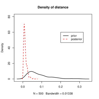
(a) Example 1: $N(0,1)$

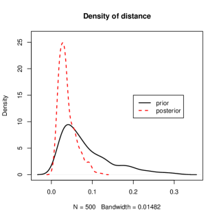
(b) Example 1: $t_{0.5}$

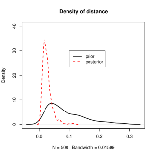
(c) Example 1: $t_{3}$

(d) Example 1: $\text{Cauchy}(0,1)$

Figure 1: Plots of prior density versus posterior density of distance for some cases in Example 1.

It is interesting to consider the effect of prior-data conflict on the methodology as this illustrates the importance of an appropriate choice of $H$ in the $DP(a,H)$ prior. Table 2 gives the outcomes of model checking for a particular sample of $n=20$ from the $N(10,1)$ distribution where $\theta(x)=10.056$ was obtained and where various choices of $H$ and $a$ are made. Clearly when $H=F_{\theta(x)}$, we get the correct conclusion about the location normal model but not otherwise even though each $H$ is in the location normal family. If $a$ is increased when $H$ is far from the truth, this increases prior-data conflict and its ill effects.

Distribution	$a$	$d_{0.05}$	$RB$ (Strength)
$N(\theta(x),1)$	$1$	$0.0166$	$17.20\,(1.00)$
	$5$	$0.0053$	$7.00\,(0.65)$
	$10$	$0.0029$	$3.20\,(0.84)$
$N(0,1)$	$1$	$0.0210$	$0.00\,(0.00)$
	$5$	$0.0053$	$0.00\,(0.00)$
	$10$	$0.0031$	$0.00\,(0.00)$
$N(9,1)$	$1$	$0.0189$	$0.04\,(0.00)$
	$5$	$0.0056$	$0.00\,(0.00)$
	$10$	$0.0033$	$0.00\,(0.00)$

Table 2: Relative belief ratios and strengths for testing the location normal model with various alternatives and choices of $a$ in Example 1 when there is prior-data conflict.

Example 2. Location-scale normal model.

In this example $\{F_{\theta}:\theta\in\Theta\}=\{N(\mu,\sigma^{2}):\theta=(\mu,\sigma^{2})\in\mathcal{\mathbb{R}}\times(0,\infty)\}$ and so $\theta(x)=(\bar{x},\sum_{i=1}^{n}(x-\bar{x})^{2}/n).$ The results are reported in Table 3. It is seen that in all cases where the normal is correct the methodology gives the correct answer. Failures occur with the mixture of normals and the $U[-1,1]$ distributions, as evidence is not obtained against the model in these cases. In these cases the Cramér-von Mises distance does not appear to give a particularly powerful test against these alternatives. When the sample size $n$ and $a$ are increased, however, model failure is detected. For example, with $n=100$ and $a=20,$ the relevant relative belief ratios (strengths) are $0.64\,(0.09)$ and $0.60\,(0.082)$ for the mixture of normals and $U[-1,1]$ distributions, respectively. So reasonably strong evidence is obtained against normality in both cases and even more conclusive results are obtained with $a=25,$ namely, $0.52(.06)$ and $0.16\,(0.02),$ respectively.

Distribution	$d_{min}$	$a$	$d_{0.05}$	$RB$ (Strength)
$N(0,1)$	$0.0000$	$1$	$0.0189$	$17.52\,(1.00)$
		$5$	$0.0061$	$9.44\,(1.00)$
		$10$	$0.0035$	$3.84\,(1.00)$
$N(10,1)$	$0.0000$	$1$	$0.0172$	$18.12\,(1.00)$
		$5$	$0.0057$	$10.52\,(1.00)$
		$10$	$0.0035$	$4.72\,(1.00)$
$N(0,4)$	$0.0000$	$1$	$0.0192$	$15.40\,(1.00)$
		$5$	$0.0064$	$5.24\,(1.00)$
		$10$	$0.0033$	$1.92(0.792)$
$N(0,9)$	$0.0000$	$1$	$0.0184$	$15.88\,(1.00)$
		$5$	$0.0034$	$3.00\,(0.382)$
		$10$	$0.0030$	$1.44\,(0.362)$
$0.5N(-2,1)+0.5N(2,1)$	$0.0462$	$1$	$0.0191$	$16.52\,(1.00)$
		$5$	$0.0055$	$4.60\,(0.77)$
		$10$	$0.0030$	$2.28\,(0.75)$
$t_{0.5}$	$0.0575$	$1$	$0.0182$	$0.00\,(0.00)$
		$5$	$0.0057$	$0.00\,(0.00)$
		$10$	$0.0032$	$0.00\,(0.00)$
$t_{3}$	$0.0120$	$1$	$0.0187$	$13.84\,(0.308)$
		$5$	$0.0062$	$4.68\,(0.766)$
		$10$	$0.0031$	$0.96\,(0.356)$
$\text{Cauchy}(0,1)$	$0.0335$	$1$	$0.0198$	$0.00\,(0.00)$
		$5$	$0.00596$	$0.00\,(0.00)$
		$10$	$0.0031$	$0.00\,(0.00)$
$U[0,1]$	$0.0246$	$1$	$0.0181$	$17.68\,(1.00)$
		$5$	$0.0060$	$10.56\,(1.00)$
		$10$	$0.0032$	$1.00\,(0.00)$
$U[-1,1]$	$0.0245$	$1$	$0.0150$	$17.6\,(0.12)$
		$5$	$0.0051$	$8.68\,(1.00)$
		$10$	$0.0031$	$6\,.00\,(0.70)$
$exp(1)$	$0.0567$	$1$	$0.0018$	$0.12\,(0.01)$
		$5$	$0.0053$	$0.04\,(0.00)$
		$10$	$0.0030$	$0.00\,(0.00)$
$exp(10)$	$0.0567$	$1$	$0.0170$	$0.20\,(0.00)$
		$5$	$0.0055$	$0.24\,(0.02)$
		$10$	$0.0032$	$0.20\,(0.01)$

Table 3: Relative belief ratios and strengths for testing the location-scale normal model with various alternatives and choices of $a$ in Example 2.

Consider now the data of 100 stress-rupture lifetimes of Kevlar pressure vessels presented in Andrews and Herzberg (1985). The goal is to test whether the underlying distribution is normal. In this case $\theta(x)=(209.171,37606.56)$. Previous studies such as Evans and Swartz (1994) and Verdinelli and Wasserman (1998), suggested that model is not correct. In this case $\inf_{\theta\in\Theta}d_{CvM}\left(F_{n},F_{\theta}\right)=$ $0.0494$, which is relatively a small distance, while $d_{CvM}\left(F_{n},F_{\theta(x)}\right)=0.0928$. The results in Table 4 support somewhat the non-normality of this data set although only when using a more concentrated prior. Figure 2 provides plots of the prior and posterior densities of the distance for various values of the concentration parameter $a$. It follows clearly from this figure that increasing the concentration parameter $a$ makes the density of the prior distance more concentrated about $0$ than the density of the posterior distance. Thus, Figure 2 supports the conclusion of the non-normality of the data set.

$a$	$d_{0.05}$	$RB$ (Strength)
$1$	$0.0175$	$18.68\,(1.00)$
$5$	$0.0059$	$4.96\,(1.00)$
$10$	$0.0030$	$0.56\,(0.02)$
$15$	$0.0023$	$0.28\,(0.01)$
$20$	$0.0016$	$0.08\,(0.01)$

Table 4: Relative belief ratios and strengths for testing the normality of the Kevlar data using various choices of $a$ in Example 2.

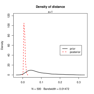
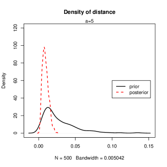
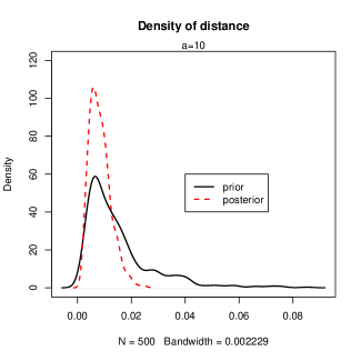
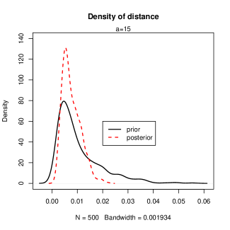
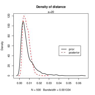
Figure 2: (a) Plots of the prior and posterior densities of the distance for the stress-rupture lifetimes of Kevlar pressure vessels data set discussed in Example 2 using various values of the concentration parameter $a$.

Example 3. Scale-exponential model.

In this example $\{F_{\theta}:\theta\in\Theta\}=\{\exp(\theta):\theta\in(0,\infty)\mathcal{\}}$ and so $\theta(x)=\bar{x}.$ The results are reported in Table 5 and it is seen that the methodology performs very well here. In fact, the model is always correctly identified when it is true and always strong evidence is obtained against the model when it is false except when considering the $U[0,1]$ distribution with $a=1$ but the more concentrated prior leads to evidence against.

Distribution	$d_{min}$	$a$	$d_{0.05}$	$RB$ (Strength)
$N(0,1)$	$0.2287$	$1$	$0.0176$	$0.00\,(0.00)$
		$5$	$0.0054$	$0.00\,(0.00)$
		$10$	$0.0030$	$0.00\,(0.00)$
$N(10,1)$	$0.2780$	$1$	$0.0188$	$0.00\,(0.00)$
		$5$	$0.0056$	$0.00\,(0.00)$
		$10$	$0.0033$	$0.00\,(0.00)$
$N(0,4)$	$0.2291$	$1$	$0.0189$	$0.00\,(0.00)$
		$5$	$0.0051$	$0.00\,(0.00)$
		$10$	$0.0029$	$0.00\,(0.00)$
$N(0,9)$	$0.2292$	$1$	$0.01730$	$0.00\,(0.00)$
		$5$	$0.0063$	$0.00\,(0.00)$
		$10$	$0.0031$	$0.00\,(0.00)$
$0.5N(-2,1)+0.5N(2,1)$	$0.2148$	$1$	$0.0179$	$0.00\,(0.00)$
		$5$	$0.0057$	$0.00\,(0.00)$
		$10$	$0.0033$	$0.00\,(0.00)$
$t_{0.5}$	$0.2385$	$1$	$0.0187$	$0.00\,(0.00)$
		$5$	$0.0056$	$0.00\,(0.00)$
		$10$	$0.00284$	$0.00\,(0.00)$
$t_{3}$	$0.2303$	$1$	$0.0186$	$0.00\,(0.00)$
		$5$	$0.0055$	$0.00\,(0.00)$
		$10$	$0.0031$	$0.00\,(0.00)$
$\text{Cauchy}(0,1)$	$0.2336$	$1$	$0.0181$	$0.00\,(0.00)$
		$5$	$0.0053$	$0.00\,(0.00)$
		$10$	$0.0031$	$0.00\,(0.00)$
$U[0,1]$	$0.0811$	$1$	$0.0202$	$3.60\,(1.00)$
		$5$	$0.0060$	$0.20\,(0.00)$
		$10$	$0.0030$	$0.08\,(0.01)$
$U[-1,1]$	$0.2266$	$1$	$0.0200$	$0.00\,(0.00)$
		$5$	$0.0060$	$0.00\,(0.00)$
		$10$	$0.0033$	$0.00\,(0.00)$
$exp(1)$	$0$	$1$	$0.0173$	$12.88\,(0.37)$
		$5$	$0.0063$	$4.76\,(1.00)$
		$10$	$0.0032$	$2\,(1.00)$
$exp(10)$	$0$	$1$	$0.0185$	$16.88\,(1.00)$
		$5$	$0.0057$	$4.40\,(0.78)$
		$10$	$0.0030$	$1.16\,(0.30)$

Table 5: Relative belief ratios and strengths for testing the scale exponential model with various alternatives and choices of $a$ in Example 3.

8 Conclusions

A general methodology for model checking based on the use of the Dirichlet process and relative belief has been considered. This combination is seen to lead to some unique advantages for this problem and this has been demonstrated by developing theoretical properties of the procedure. Through several examples, it has been shown that the approach performs extremely well.

While Cramér-von Mises distance has been used here, other distance measures could be used instead and may have distinct advantages in some problems. For instance, the Anderson-Darling distance and the Kullback-Leibler distance are possible substitutes. This entails simply substituting such alternatives for $d_{CvM}$ in the algorithms. An important extension is the generalization of the approach to construct tests for families of multivariate distributions. While conceptually similar, there are computational and inferential issues that need to be addressed and this is the subject of current research.

9 References

Al-Labadi, L., and Zarepour, M. (2013). A Bayesian nonparametric goodness of fit test for right censored data based on approximate samples from the beta–Stacy process. Canadian Journal of Statistics, 41, 3, 466–487.

Al-Labadi, L., and Zarepour, M. (2014). Goodness of fit tests based on the distance between the Dirichlet process and its base measure. Journal of Nonparametric Statistics, 26, 341-357.

Andrews, D. F. and Herzberg, A. M. (1985) Data - A Collection of Problems from Many Fields for the Student and Research Worker. Springer.

Baskurt, Z. , and Evans, M. (2013). Hypothesis assessment and Inequalities for Bayes factors and relative belief ratios. Bayesian Analysis, 8, 3, 569-590.

Berger, J. O., and Guglielmi, A. (2001). Bayesian testing of a parametric model versus nonparametric alternatives. Journal of the American Statistical Association, 96, 174–184.

Bondesson, L. (1982). On simulation from infinitely divisible distributions. Advances in Applied Probability, 14, 885-869.

Carota, C., and Parmigiani, G. (1996). On Bayes factors for nonparametric alternatives. In Bayesian Statistics 5 (J. M. Bernardo, J. . Berger, A. P. Dawid, and A. F. M., eds.) Smith. Oxford University Press, London.

Choi, K. , and Bulgren, W. G. (1988). An estimation procedure for mixtures of distributions. Journal of the Royal Statistical Society, B, 30, 444–460.

Dasgupta, A. (2008). Asymptotic Theory of Statistics and Probability. Springer, New York.

Evans, M. (2015). Measuring Statistical Evidence Using Relative Belief. Monographs on Statistics and Applied Probability 144, CRC Press, Taylor & Francis Group.

Evans, M. and Moshonov, H. (2006). Checking for prior-data conflict. Bayesian Analysis, 1, 4, 893-914.

Evans, M. and Swartz, T. (1994). Distribution theory and inference for polynomial-normal densities. Communications in Statistics–Theory and Methods, 23, 1123–1148.

Ferguson, T. S. (1973). A Bayesian analysis of some nonparametric problems. Annals of Statistics, 1, 209-230.

Florens, J. P., Richard, J. F., and Rolin, J. M. (1996). Bayesian encompassing specification tests of a parametric model against a nonparametric alternative. Technical Report 9608, Universitsé Catholique de Louvain, Institut de statistique.

Gibbs, A., and Su, E. F. (2002). On choosing and Bounding Probability metrics. International Statistical Review, 70, 419-435.

Hsieh, P. (2011). A nonparametric assessment of model adequacy based on Kullback–Leibler divergence. Statistics and Computing, 23, 149–162.

Ishwaran, H., and Zarepour, M. (2002). Exact and Approximate Sum Representations for the Dirichlet Process. The Canadian Journal of Statistics, 30, 269-283.

James, L. F. (2008). Large sample asymptotics for the two-parameter Poisson-Dirichlet process. In Pushing the Limits of Contemporary Statistics: Contributions in Honor of Jayanta K. Ghosh, ed. B. Clarke and S. Ghosal, Ohio: Institute of Mathematical Statistics, 187-199.

Lavine, M. (1992). Some aspects of Pólya tree distributions for statistical modelling. Annals of Statistics, 20, 1222–1235.

McVinish, R., Rousseau, J., and Mengersen, K. (2009). Bayesian goodness of fit testing with mixtures of triangular distributions. Scandivavian Journal of Statistics, 36, 337–354.

Sethuraman, J. (1994). A constructive definition of Dirichlet priors. Statistica Sinica, 4, 639-650.

Swartz, T. B. (1999). Nonparametric goodness–of–fit. Communications in Statistics: Theory and Methods, 28, 2821–2841.

Verdinelli, I., and Wasserman, L. (1998). Bayesian goodness-of-fit testing using finite-dimensional exponential families. Annals of Statistics, 26, 1215–1241.

Viele, K., (2000). Evaluating fit using Dirichlet processes. Technical Report 384, University of Kentucky, Dept. of Statistics.

Wolpert, R. L., and Ickstadt, K., (1998). Simulation of Lévy random fields. In Practical Nonparametric and Semiparametric Bayesian Statistics, ed. D. Day, P. Muller, and D. Sinha, Springer, 227-242.

Zarepour, M., and Al-Labadi, L. (2012). On a rapid simulation of the Dirichlet process. Statistics & Probability Letters, 82, 5, 916-924.