In Situ and Ex Situ Formation Models of Kepler 11 Planets
Abstract
We present formation simulations of the six Kepler 11 planets. Models assume either in situ or ex situ assembly, the latter with migration, and are evolved to the estimated age of the system, . Models combine detailed calculations of both the gaseous envelope and the condensed core structures, including accretion of gas and solids, of the disk’s viscous and thermal evolution, including photo-evaporation and disk-planet interactions, and of the planets’ evaporative mass loss after disk dispersal. Planet-planet interactions are neglected. Both sets of simulations successfully reproduce measured radii, masses, and orbital distances of the planets, except for the radius of Kepler 11b, which loses its entire gaseous envelope shortly after formation. Gaseous (H+He) envelopes account for % of the planet masses, and between and % of the planet radii. In situ models predict a very massive inner disk, whose solids’ surface density () varies from over to at stellocentric distances . Initial gas densities would be in excess of if solids formed locally. Given the high disk temperatures (), planetary interiors can only be composed of metals and highly refractory materials. Sequestration of hydrogen by the core and subsequent outgassing is required to account for the observed radius of Kepler 11b. Ex situ models predict a relatively low-mass disk, whose initial varies from to at and whose initial gas density ranges from to . All planetary interiors are expected to be rich in H2O, as core assembly mostly occurs exterior to the ice condensation front. Kepler 11b is expected to have a steam atmosphere, and H2O is likely mixed with H+He in the envelopes of the other planets. Results indicate that Kepler 11g may not be more massive than Kepler 11e.
Subject headings:
Planetary systems – Planets and satellites: formation – Planets and satellites: individual (Kepler 11) – Planets and satellites: interiors – Protoplanetary disks – Planet-disk interactions1. Introduction
Numerous planetary systems have been discovered that consist of two or more planets with masses of a few Earth masses (), orbiting in the same plane within of the central star (e.g. Figueira et al., 2012; Mullally et al., 2015). Some properties of such systems are reviewed by Winn & Fabrycky (2015). A particularly well-studied example is the Kepler 11 system, with a central solar-type star (age ) and six orbiting planets with semi-major axes ranging from to . Their radii, measured through transit observations from the Kepler spacecraft, are – Earth radii (), placing them in the super-Earth/sub-Neptune size range. Estimates of their masses have been obtained from transit timing measurements (Lissauer et al., 2013, hereafter L13); for the five inner planets, the values range from to (see also Borsato et al., 2014; Hadden & Lithwick, 2014). All of these inner planets have densities that are substantially less than that of a rocky planet, implying that they could each be composed of a heavy-element core surrounded by a gaseous envelope. In the cases of planets c, d, e, and f, these envelopes are most likely composed of hydrogen and helium, in roughly solar proportions, while Kepler 11b’s envelope could be composed either of H+He or H2O steam (Lopez et al. 2012; L13). The estimated mass fractions of these envelopes range from % in the case of Kepler 11b to % for Kepler 11e (see also Lopez et al. 2012 L13). However, their volumes are substantial and play an important role in determining the observed planet radii.
One of the main issues pertinent to the understanding of this system is the formation history of the planets. While it is generally assumed that these planets formed by core-nucleated accretion (Safronov, 1969), the formation location is not well established. Several studies have proposed that planets in systems of this type formed in situ (e.g., Hansen & Murray, 2012, 2013; Ikoma & Hori, 2012; Chiang & Laughlin, 2013; Tan et al., 2015) and analytic estimates of the envelope-to-core mass ratio in the relevant mass range have also been made (Lee & Chiang, 2015; Ginzburg et al., 2016). Other simulations support the alternative ex situ assumption, that is, that the planets formed farther out in the disk and, during or after formation, migrated inward to their present positions through interactions with the protoplanetary disks (e.g., McNeil & Nelson, 2010; Rogers et al., 2011; Lopez et al., 2012; Mordasini et al., 2012; Bodenheimer & Lissauer, 2014; Hands et al., 2014; Chatterjee & Ford, 2015). The physical mechanisms involved in the process of orbital migration via disk-planet tidal interactions are reviewed by Kley & Nelson (2012) and Baruteau et al. (2014, pp. 667-689).
While the in situ model has been favored because the terrestrial planets in the solar system presumably formed in this way, the migration (or ex situ) model has been favored because of the difficulties in forming planets in situ in the very inner regions of disks (Bodenheimer et al., 2000), well inside the orbit of Mercury in the solar system. However, a significant argument against the ex situ picture is that in a multiple system, if the planets had undergone convergent migration, they would be expected to have been captured into mean-motion resonances (e.g., Lissauer et al., 2011a), while in fact most of the systems observed by Kepler do not appear to be in resonance. Goldreich & Schlichting (2014) discuss a mechanism, involving an instability in resonances, that would allow the planets to move through resonances; therefore, migration is not ruled out. Deck & Batygin (2015) revisit this problem and conclude that although the instability in resonances is indeed possible, the time spent by a planet pair in resonance exceeds by a considerable amount the time during which the planets are out of resonance. Thus, they argue that the Goldreich & Schlichting process does not solve the problem that most Kepler planet pairs are not in resonance. However, there are other mechanisms that could move planets out of resonance, including dissipative effects (Delisle et al., 2012; Lithwick & Wu, 2012; Batygin & Morbidelli, 2013), stochastic effects during migration (Rein, 2012), tidal effects caused by planet-wake interactions (Baruteau & Papaloizou, 2013) and the effects of small eccentricities in the planetary orbits (Batygin, 2015). Moreover, the highly complex orbital architecture of compact multiple systems, as in the case of Kepler 11, may indeed require a migration-based formation scenario (Migaszewski et al., 2012). Nevertheless, there are still many other uncertainties in the theory of planet-disk interactions, as discussed in more detail by Chiang & Laughlin (2013) and Kley & Nelson (2012), leading to legitimate questioning of whether the theoretical processes of planet formation with migration can explain the mass distribution as well as the orbital period distribution of super-Earth/sub-Neptune planets (Howard et al., 2010).
On the other hand, there are several difficulties with the picture of in situ formation of super-Earths/sub-Neptunes. First, even if the planets did form by this process, they still would be subject to orbital decay. If migration is included in simulations of in situ super-Earth formation (Ogihara et al., 2015), the semi-major axis distribution of planets does not agree with the distribution observed by Kepler. Agreement is possible only if orbital migration is suppressed. Second, for the specific case of the Kepler 11 system, a very high surface density of solid material in the inner disk is required, well above that of the minimum-mass solar nebula and even above that of minimum-mass extrasolar nebulae (Chiang & Laughlin, 2013; Schlichting, 2014). This problem may be alleviated if it is assumed that solid material migrates inwards from the outer disk, in the form of either protoplanetary cores (Ward, 1997), planetesimals (Hansen & Murray, 2012), or small pebbles (Tan et al., 2015), and collects at the appropriate locations. Third, Kepler data show an excess of planet pairs just exterior of the 2:1 and 3:2 mean-motion resonances, compared to the pairs just interior to these resonances (Lissauer et al., 2011b; Fabrycky et al., 2014; Chatterjee & Ford, 2015), which is not easily accountable by in situ formation. Fourth, it has often been assumed that in the inner disk the temperatures are too high for an appreciable concentration of solid material to exist. In fact, the simple assumption that the ratio of sound speed to orbital speed, i.e., the ratio of disk scale height to radial distance, , is at gives a temperature of about for a solar-mass central star. However, this objection is not necessarily significant. Many disk models give cooler temperatures at –. The evolving two-dimensional models of Dodson-Robinson et al. (2009) give mid-plane temperatures in the inner disk of about at an age of years, with cooling at later times. The models of Chiang & Goldreich (1999) give even cooler temperatures in the disk interior at these distances.
This paper considers all the observed planets in the Kepler 11 system and asks whether they formed in situ or ex situ, i.e., including orbital migration. In spite of the difficulties mentioned above, both of these possibilities remain viable options. Detailed formation and evolution models are numerically simulated for both scenarios with the same or very similar physical assumptions used in the construction of the planet models. In both cases, the simulations are advanced to an age of , where the computed masses, radii, and semi-major axes are compared with observations. The general physical and numerical aspects of the calculations are reported in Section 2. The in situ and ex situ models are presented, respectively, in Section 3 and 4 while results are discussed in Section 5. The conclusions are drawn in Section 6.
2. Numerical Procedures
| Symbol | Definition |
|---|---|
| Planet’s condensed core mass; Section 2.1 | |
| Planet’s condensed core radius; Section 2.1 | |
| Accretion radius; Equation (1) | |
| Planet’s Bondi radius; Equation (1) | |
| Planet’s Hill radius; Equation (1) | |
| Planet total luminosity; Equation (2) | |
| Planet effective temperature; Equation (2) | |
| Planet radius; Equation (2) | |
| Planet mass; Equation (3) | |
| Rosseland mean opacity; Equation (3) | |
| Pressure; Equation (3) | |
| Irradiation equilibrium temperature; Equation (4) | |
| Stellar effective temperature; Equation (5) | |
| Stellar radius; Equation (5) | |
| Planet orbital radius; Equation (5) | |
| Planet’s gaseous envelope mass; Section 2.1 | |
| Planet’s mass accretion rate of gas; Section 2.1 | |
| Planet’s mass accretion rate of solids; Equation (6) | |
| Disk’s surface density of solids; Equation (6) | |
| Orbital frequency; Equation (6) | |
| Gravitational enhancement factor; Equation (6) | |
| Stellar mass; Equation (7) | |
| Stellar luminosity; Section 2.3 | |
| Gas mass-loss rate during isolation; Equation (8) | |
| XUV radiation flux during isolation; Equation (8) | |
| XUV radiation absorption radius; Equation (8) | |
| XUV absorption efficiency; Equation (8) | |
| Stellocentric distance; Equation (9) | |
| Disk’s surface density of gas; Equation (9) | |
| Gravitational torque; Equation (9) | |
| Viscous torque; Equation (9) | |
| Gas kinematic viscosity; Equation (10) | |
| Temperature; Equation (14) | |
| Irradiation temperature; Equation (15) | |
| Disk scale height; Equation (16) | |
| Scattering rate of solids; Equation (18) | |
| Disk photo-evaporation rate; Equation (23) | |
| Critical radius for photo-evaporation; Section 2.6 |
In this section, we outline the numerical methods applied in the models presented herein, highlighting major differences between in situ and ex situ calculations. As a reference, Table 1 contains a list of some of the symbols used in the paper and the equation in which they appear or the section in which they are first mentioned (physical constants are omitted). In order to simplify labels, some quantities apply to both the disk and the planet, e.g., for gas temperature or for the Rosseland mean opacity, and shall be distinguished by the context in which they are used.
2.1. Envelope Structure Calculation
The calculation of the structure and evolution of the planetary gaseous envelope is based on the assumption that the envelope is spherically symmetric around its center and evolves through states of hydrostatic equilibrium (e.g., Kippenhahn et al., 2013). The envelope lies on a core of condensed matter, whose total mass and radius are both functions of time. The core radius is determined as explained below. The envelope structure is calculated by solving the equations for mass conservation, hydrostatic equilibrium, energy conservation, and radiation diffusion (see Bodenheimer & Pollack, 1986). The energy equation includes heating produced by in-falling planetesimals, the work done by gravity, cooling from the release of internal heat, and heating by stellar radiation (when applicable). In convective unstable shells, where the radiative temperature gradient exceeds in magnitude the adiabatic gradient (Kippenhahn et al., 2013), the actual gradient of temperature is set equal to the adiabatic gradient.
The chemical composition of the envelope gas is assumed to be uniform, with hydrogen and helium mass fractions and , respectively. The equation of state for this gas mixture is that computed by Saumon et al. (1995), which accounts for the partial degeneracy of electrons and for non-ideal effects in the gas. (Strictly speaking, this equation of state neglects heavier elements and uses .)
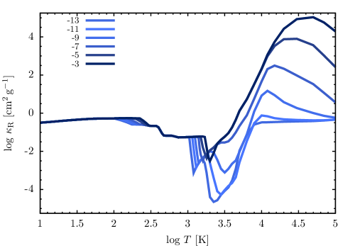
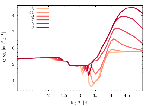
The envelope opacity arises from the combined contributions of dust, atoms, and molecules. Dust opacities are calculated as described in D’Angelo & Bodenheimer (2013), assuming the presence of a number of different grain species, and grain size distributions with a minimum radius of and a maximum radius of or . The number density of dust grains is proportional to the power of the grain radius. Low-temperature gas opacities are taken from Ferguson et al. (2005), whereas high-temperature gas opacities are taken from the OPAL tables (Iglesias & Rogers, 1996). Figure 1 illustrates the Rosseland mean opacity for the two grain size distributions considered here, along with gas opacity. Dust grains are supposed to be present in the envelope only if solids are supplied via gas and/or planetesimal accretion. In the absence of a steady supply, dust grains quickly sediment to deeper layers and evaporate. When this happens, i.e., during phases of zero gas and solids’ accretion, low-temperature opacities are replaced with the molecular opacities of Freedman et al. (2008).
The planetary evolution code is largely the same as that used by Pollack et al. (1996), Bodenheimer et al. (2000), Hubickyj et al. (2005), and Lissauer et al. (2009). The structure equations are solved by means of the Henyey method (e.g., Bodenheimer et al., 2006), supplemented with boundary conditions at the core-envelope interface, , and at the top of the envelope, . At , the mass is set equal to and the luminosity is set to zero (i.e., there is no energy flux through the core-envelope interface, see the discussion in Bodenheimer & Lissauer, 2014). The planet radius, , is assumed to have an upper bound , the accretion radius, defined by
| (1) |
where and are the Hill and Bondi radius, respectively. The limiting envelope radii, and , were estimated from first principles by means of three-dimensional (3D) calculations of the flow dynamics around planets in disks (Lissauer et al., 2009; D’Angelo & Bodenheimer, 2013).
At early stages of evolution, the planet is “in contact” with the disk (the so-called nebular stage), and the density and temperature at the top of the envelope are taken as the local disk values. During the nebular stage, gas is added to the envelope in order to restore the condition (see Pollack et al., 1996). Once this condition can no longer be maintained, the envelope contracts inside , entering a transition stage, which coincides with the run-away gas accretion phase if the gas accretion rate is sufficiently large. In fact, the gas accretion rate of the envelope, , is limited by the maximum rate at which the disk can deliver gas to the planet’s vicinity. If tidal perturbations by the planet are negligible, the disk-limited accretion rate can be described in terms of simple analytical arguments (D’Angelo & Lubow, 2008). If tidal perturbations are not negligible, the problem becomes highly complex and depends on the interplay among viscous torques, tidal torques, and close-range flow dynamics around the planet. Disk-limited accretion rates were derived from 3D hydrodynamics high-resolution calculations, as described in Bodenheimer et al. (2013), extending the parameter space covered by the fitting functions reported therein to include a larger disk viscosity range. It is important to stress that cannot exceed the disk-limited accretion rate, and there are instances in which this limit sets in during the nebular stage of evolution. The boundary conditions applied at during the transition stage are discussed in Bodenheimer et al. (2000).
Eventually, the disk’s gas around the planet’s orbit is dispersed, typically via photo-evaporation by stellar radiation, gas supply ceases, and the planet enters the isolation stage. Note that the process of gap formation in the disk by tidal torques alone, under typical disk conditions of viscosity and temperature and for planetary masses up to several times Jupiter’s mass (), does not lead to isolation (e.g., D’Angelo & Lubow, 2008; Bodenheimer et al., 2013, and references therein). During the isolation stage, standard photospheric boundary conditions are applied at (e.g., Cox, 1968)
| (2) | |||||
| (3) |
where is the Stefan-Boltzmann constant, is the gravitational constant, and and are, respectively, the photospheric values of the Rosseland mean opacity and pressure. In Equation (2), the luminosity on the left-hand side comprises both the internal power generated by the planet and the re-radiated power that arises from the absorption of stellar radiation. Hence, the planet’s effective temperature is given by (Bodenheimer & Lissauer, 2014)
| (4) |
where depends on and on the luminosity internally generated by the planet. The equilibrium temperature is such that (e.g., Guillot, 2010)
| (5) |
which assumes full redistribution of the incident radiation. The albedo is taken as a constant equal to . In Equation (5), and are the effective temperature and the photospheric radius of the star, respectively.
In calculations that allow for orbital migration, a distinction can be made between isolation from the disk’s gas and from the disk’s solids. Isolation from the planetesimals’ disk occurs when the migration speed and , or when the solids’ surface density at the planet’s location becomes very small. Isolation from the solid disk occurs prior to isolation from the disk’s gas or shortly thereafter. However, the consequences of this delay are negligible. Thus, when a planet enters the isolation phase, it is basically isolated from both the disk’s gas and solids.
During all stages, if , mass is gradually removed from the envelope. In a more realistic context, during the nebular and transition stages, an inflated planet would lose unbound mass hydrodynamically, carried away by the surrounding disk flow (D’Angelo & Bodenheimer, 2013). This mechanism of mass loss is different from those operating during the isolation stage (see Section 2.3). As a result of gas loss, while is a monotonic function of time, and may not be.
Accretion of solids is treated as in Pollack et al. (1996). All solids accreted by the planet are assumed to sink to the core, in a condensed form, and increment the core mass. As originally derived by Safronov (1969), the accretion rate of solids can be written as
| (6) |
where is the effective cross section for planetesimal capture of the planet, is the solids’ surface density at the planet’s orbital radius, , is the planet’s orbital frequency, and is the ratio of the gravitational to the geometric cross section (Greenzweig & Lissauer, 1990, 1992), known as the gravitational enhancement factor. Further details can be found in Pollack et al. (1996, and references therein). The accretion rate in Equation (6) neglects the contribution of the dust entrained in the accreted gas (% by mass). The planetesimal radius is assumed to be , although smaller planetesimals were also tested.
A planetary embryo accreting planetesimals at a fixed orbital radius will deplete an annular region around its orbit of full width about equal to , at which point the condensed core becomes detached from the planetesimals’ disk. In these calculations, the secular evolution of planetesimals is neglected and therefore, once detached, the core reaches its final mass
| (7) |
which neglects the contribution of the envelope mass to and is hence appropriate when . The situation is more complex for a migrating planet, since the depletion rate of solids in the disk tends to be initially slower than the migration rate through the disk. Hence, the planet cuts a swathe through the solids’ disk, which deepens as reduces, eventually detaching itself. The final mass of the core in this case is more difficult to predict, as it depends on both the accretion and migration history. During the long isolation stage, a planet may be subjected to stochastic impacts, which may alter the core and envelope mass and the planet’s orbit if the impactors are sufficiently massive. This possibility is not considered here.
As mentioned above, solids sink to the top of the core. This process releases energy in the envelope, affecting the local energy budget, but not the local chemical composition of the envelope. These calculations consider accretion of hydrated, partly hydrated, and anhydrous planetesimals, depending on the local disk temperature. Rocky planetesimals may reach the core nearly intact if they are large enough (they may be held together by their own gravity) or if the ram pressure does not exceed their compressive strength (D’Angelo & Podolak, 2015, and references therein). Ice-rich planetesimals are more easily disrupted or entirely ablated in the envelope because the critical temperature of H2O is only , a value reached in relatively shallow layers of the envelope (their mass is nevertheless assumed to sink to the core).
An important part of the calculation is represented by the capture of planetesimals, which determines self-consistently the cross section in Equation (6), and by their interaction with the planet’s envelope, which determines depth-dependent mass and energy deposition rates. This part is based on the protocols described in Pollack et al. (1996), enhanced with an improved integration algorithm of the planetesimals’ trajectories (D’Angelo et al., 2014). In brief, a number of trajectories with a varying impact parameter () are integrated through the envelope. The largest impact parameter for which the body hits the core surface, breaks up, or is entirely ablated provides the radius for planetesimal capture and hence the cross section . At this point, an additional series of trajectory integrations is performed, with an impact parameter up to the capture radius, to record the ablation history and the fate of the body as a function of the impact parameter. This collective information provides the mean energy and mass deposition rates in each envelope layer.
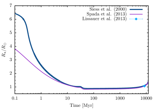

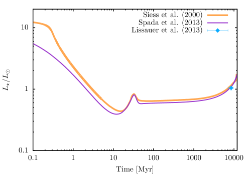
The methods outlined above apply to both in situ and ex situ calculations. The basic difference is that the boundary conditions at change over time in ex situ models, whereas in situ calculations allow only for a linear decline with time of the gas surface density at . In ex situ models, the surface density in Equation (6) also varies as a function of the distance from the star and of the disk temperature. Additionally, ex situ models use stellar properties from stellar structure models of solar-type stars to compute the equilibrium temperature (Equation (5)), the mass-loss rate during isolation (Equation (8)), and the irradiation temperature of the disk (Equation (16)). The calculations apply a stellar model of a solar-mass and protosolar metallicity ([Fe/H], Asplund et al., 2009; Lodders, 2010) star from Siess et al. (2000), whose radius, effective temperature, and luminosity are plotted in Figure 2. For comparison, some calculations are repeated by adopting a Yonsei-Yale model (Spada et al., 2013) for a , [Fe/H] star, also represented in Figure 2. In contrast, in situ models are based on fixed, solar-type values for radius, effective temperature, and luminosity of the star.
2.2. Core Structure Calculation
In situ formation calculations determine the core radius, , from its current mass, , using tables of results from Rogers et al. (2011). The core is composed of iron and silicates, with Earth-like mass fractions of % and %, respectively. Applied to an Earth-mass planet, the results predict a radius within % of the Earth radius, . The radius is then used as an inner boundary condition for the H+He envelope.
Ex situ formation calculations allow for accretion of planetesimals whose composition varies as a function of time and distance from the star. At disk temperatures below , the planetesimals are ice-rich, % by mass (% silicates and % iron). They become progressively ice-poor (and rich in silicates and iron) at higher disk temperatures and are anhydrous at temperatures above (D’Angelo & Podolak, 2015), where a terrestrial-type composition is adopted (% silicates and % iron by mass). The mass fractions of iron, silicates, and ice are linearly interpolated in temperature between and .
Since the composition of the condensed core may vary during the evolution of ex situ models, as the composition of accreted solids changes, detailed calculations of the core structure are performed. The core is assumed to be spherically symmetric about its center and described by the equation of mass conservation and hydrostatic equilibrium (see Appendix A). The core is taken to be fully differentiated into an iron nucleus, a silicate mantle, and an outer shell of condensed H2O. Two-layer (with any combination of the three materials) or one-layer structures are also possible. Each material is characterized by a “cold” equation of state (EoS) relating density and pressure. We experimented with a combination of Birch-Murnaghan, Vinet, and Generalized Rydberg EoS (for a review, see Stacey & Davis, 2008), and extend them to very high pressures by means of the Thomas-Fermi-Dirac theory. Details are given in Appendix A. Temperature effects on the EoS are neglected since thermal pressure is expected to provide only a minor correction to for the core masses considered here (see, e.g., Valencia et al., 2006; Seager et al., 2007; Sotin et al., 2007; Sohl et al., 2014b). However, temperature effects are included to account for phase transitions within the layers (see Appendix A for details). Applying this module to an Earth-mass planet with a composition of % silicates and % iron by mass, the calculated radius is within % of . For a cold-Earth analog (% silicates and % iron by mass, Sohl & Schubert, 2007, pp. 27-68), the resulting radius is within % of . More detailed structure calculations, including heat transfer and additional material phases, are also presented in Appendix A. They are compared to isothermal core structures in Appendix C.
The integration of the equations proceeds from the center outward, varying the central pressure in an iterative fashion, until the pressure at the core radius, , matches (within %) the pressure at the bottom of the envelope, which is provided by the envelope structure module (Section 2.1). The integration of the core structure equations is performed whenever increases by % or if the pressure or temperature at changes by %.
2.3. Radiation-Driven Gas Loss During Isolation
Removal of envelope gas after the planet becomes isolated, when stellar photons can directly impinge on the planet dayside, is based on the energy-limited hydrodynamics escape driven by stellar X-ray and EUV (XUV) radiation (Watson et al., 1981; Erkaev et al., 2007; Murray-Clay et al., 2009; Lopez et al., 2012). In this limit, the mass-loss rate of the envelope can be approximated as
| (8) |
where is the envelope radius at which the atmosphere becomes optically thick to the incoming stellar XUV radiation and most of the flux is absorbed (Erkaev et al., 2007; Murray-Clay et al., 2009), is a reduction factor of the planet’s potential energy caused by tidal forces of the star, and (Erkaev et al., 2007). Escape is assumed to take place at the equipotential surface passing through the collinear Lagrange point . Note that Equation (8) diverges for . During the evolution in isolation, it is assumed that .
Observations of the histories of EUV and X-ray fluxes of solar-type stars suggest that mass loss is most vigorous at ages of (Ribas et al., 2005). Here, we set for and at later times (Ribas et al., 2005), where is the stellar bolometric luminosity. The quantity is an efficiency factor intended to roughly account for radiative losses from the envelope (Erkaev et al., 2007), so that only a fraction of the incident flux can effectively drive mass loss. This factor is quite uncertain. These calculations are based on an efficiency of (e.g., Murray-Clay et al., 2009; Lopez et al., 2012). However, other values of are considered for a sensitivity study.
In situ and ex situ calculations handle radiation-induced mass loss of the envelope in similar ways. The only basic difference is that, in Equation (8) and in the function , replaces in the in situ models. Additionally, the stellar luminosity of ex situ models varies in time, according to the applied stellar evolution model (see Figure 2), whereas in situ simulations use . Since the XUV stellar output is assumed to be proportional to , the mass-loss history of the envelope during isolation may differ from that occurring at a constant value of , as used by in situ calculations.
Other mass-loss mechanisms during the beginning of the isolation phase have been considered. Ikoma & Hori (2012) and Ginzburg et al. (2016) studied the effect of loss of pressure support at the planet’s outer boundary once the disk’s gas disperses; the energy for the mass loss is supplied by the planet’s cooling luminosity. Owen & Wu (2016) considered a similar mechanism, initiated by the loss of pressure from the disk, in which a “Parker” wind is driven by a combination of the stellar continuum radiation and the gravitational energy released as the planet contracts. The assumptions made in these works are considerably different from those made here, and it is not clear if these processes would be significant in our models. First, the planet radius in the above papers is implicitly assumed to be close to , while in the models discussed here, just before disk dispersal, is roughly a factor of to smaller than (see also Section 3). Second, as the disk disperses, the possible up-lifting of the outer envelope layers due to loss of disk pressure during the nebular stage is implicitly included in the structure calculation through the boundary conditions at . After disk dispersal, the boundary conditions transition to those of an isolated photosphere (Equations (2) and (3)). The transition occurs on the cooling timescale of the outer envelope layers, which is shorter than the disk dispersal timescale. As a result, the photospheric pressure increases and the planet further contracts inside . The Owen & Wu mechanism, for example, is not significant for . Clearly, whether these wind mechanisms are in fact unimportant in calculations like ours needs to be tested in more detail.
2.4. Disk Evolution
These models consider the evolution of an axisymmetric gaseous disk, of surface density , driven by turbulence viscosity (of some nature), stellar-induced photo-evaporation, tidal torques due to gravitational interactions with an embedded planet, and accretion of gas on the planet. Indicating with the viscous torque acting between two adjacent disk’s annuli at a distance from the star and with the tidal torque exerted by the planet on the disk’s gas at radius , conservation of mass and momentum within the disk leads to the following disk’s evolution equation (e.g., Lin & Papaloizou, 1986)
| (9) |
where is the disk’s rotation rate, is gas mass removed by photo-evaporation per unit disk surface and unit time (see Section 2.6), and is gas mass removed by accretion on the planet per unit disk surface and unit time. Recalling that (Lynden-Bell & Pringle, 1974) and approximating to the Keplerian rotation rate , the viscous torque becomes and Equation (9) assumes the more familiar form
| (10) | |||||
The quantity is the torque density distribution, i.e., the gravitational torque per unit disk mass () arising from tidal interactions with the planet. This function is discussed in Section 2.5. If multiple planets orbit in the disk, is the sum of all partial torque density distributions. The presence of the tidal torque term in Equation (10) naturally accounts for (planet-induced) gap formation in the density distribution. Notice that, if is constant in radius, a viscously evolving planet-less disk is in a steady state.
The mass removed from the disk, via accretion on the planet, per unit surface and unit time, is written as so that , the planet’s gas accretion rate, which ensures conservation of the mass transferred between the planet and the disk. Contrary to (which is zero or positive), can be positive, null, or negative. In the latter case, mass is transferred from the planet to the disk. The planet’s envelope can lose mass () if its radius exceeds the accretion radius (see Section 2.1). Numerically, to avoid discontinuities, the mass added to (removed from) the planet is removed from (added to) a disk region around the planet’s orbit of radial width a few times .
The presence of an accreting planet can change the mass transfer through the disk and thus alter the disk’s surface density (Lubow & D’Angelo, 2006). This effect cannot be described by Equation (10). To account for it, the approach of Lubow & D’Angelo (2006) is applied. The accretion rate through the disk is (adopting the convention that for an inward transfer of mass). By indicating with and accretion rates averaged over narrow rings, respectively, exterior and interior to the planet’s orbit (and sufficiently apart from it), the condition is imposed that
| (11) |
Equation (11) is used to adjust (i.e., ) inside and outside of the planet’s orbit in a mass-conservative manner. This correction is applied only if . For stability reasons, mass adjustments are spread over several grid zones.
The thermal structure of the disk is determined by imposing a simple energy balance involving viscous heating, radiative cooling from the surface of the disk, and irradiation heating by the star
| (12) |
In the case of Keplerian rotation, the energy flux produced by viscous dissipation is (Mihalas & Weibel Mihalas, 1999)
| (13) |
The energy flux escaping from the disk’s surface and the heating flux generated by stellar photons are (Hubeny, 1990)
| (14) |
and
| (15) |
respectively. In the equations above, is the mid-plane temperature of the disk, is the stellar irradiation temperature, and and are the Rosseland and Planck mean opacities. These opacity coefficients are calculated following the method of D’Angelo & Bodenheimer (2013), for grain size distributions of up to in radius, and connected to the gas opacities of Ferguson et al. (2005). The advantage of using the fluxes in Equations (14) and (15) is that, in the approximation of vertically integrated quantities, they also describe optically thin disks. The irradiation temperature is written as (e.g., Menou & Goodman, 2004)
| (16) |
The disk scale height, assuming vertical hydrostatic equilibrium, is given by . The adiabatic index is set between and and the mean molecular weight is ( is the Boltzmann constant and the hydrogen mass). Equation (16) includes the contribution from luminosity released by accretion on the star (Pringle, 1981)
| (17) |
The stellar accretion rate is computed as , from the solution of Equation (10) at the inner boundary of the disk (where ).
The disk also contains a solid component, assumed to be formed of -radius planetesimals, whose surface density is . In principle, this planetesimal disk would evolve through gravitational encounters, including collisions, and interactions with any embedded planet. Gas drag would also affect the evolution of this solid component, but over rather long timescales, given the size of the bodies considered here. However, for the sake of simplicity and tractability, it is assumed that only varies because of depletion by accretion of solids on the planet () and because of scattering by the planet’s gravity (Ida & Lin, 2004)
| (18) |
The equation above is a very simple approximation, based on energy arguments, and assumes that , which is appropriate for the planets modeled here. The surface density also changes in response to temperature variations in the disk, allowing for the vaporization of ice (see Section 2.2).
Equation (10) is solved by means of a hybrid implicit/explicit numerical scheme, based on the fourth/fifth-order Dormand-Prince method (embedding backward differentiation) with an adaptive step-size control for the global accuracy of the solution (Hairer et al., 1993). Additional details and tests can be found in D’Angelo & Marzari (2012). Toward the end of the disk’s life, when the evolution is entirely driven by photo-evaporation and the disk is quickly dispersed, the algorithm transitions from implicit to explicit, with a time step condition that constrains the maximum amount of mass removed from any disk annulus. Details on the solution method of Equation (12) for the energy balance are also given in D’Angelo & Marzari (2012). The disk extends in radius from the larger of and to , and is discretized over grid points by imposing a constant ratio . Beyond , to ensure that the grid boundary does not interfere with viscous spreading, a buffer zone of additional grid points (at a degraded resolution) brings the outer disk edge to .
2.5. Tidal Interactions and Orbital Migration
In order to describe tidal interactions between the disk and the planet, we apply the formalism of D’Angelo & Lubow (2008, 2010) for local isothermal disks. This is based on the torque density distribution, which is defined by the integral
| (19) |
where is the total torque applied to the planet. In actuality, the integral is performed over the disk’s radial extent. In a disk whose properties vary smoothly with radius, the theory of disk resonances (e.g., Meyer-Vernet & Sicardy, 1987; Ward, 1997) suggests that
| (20) |
where is a dimensionless parametric function of with , whose extrema are at . The parameters and are calculated as averages between and (the function is practically zero outside of these limits). D’Angelo & Lubow (2010, hereafter DL10) tested the validity of Equation (20) and provided analytic approximations of the function , for wide ranges of the parameters and , based on 3D hydrodynamics calculations of disk-planet interactions.
Gravitational interactions transition from a linear to a nonlinear regime when , or
| (21) |
Nonlinear interactions can cause order-of-magnitude variations in the surface density (relative to the unperturbed disk), as the planet mass grows. However, under typical disk conditions, the torque density varies smoothly across the transition, and the maximum and minimum of the function change only by factors of the order of unity. The variation of across the transition is implemented as explained in DL10.
The rate of change of the planet’s orbital radius is found by imposing conservation of orbital angular momentum, which yields . Since is defined through Equation (19), the migration speed becomes
| (22) | |||||
where the integration is performed over the entire disk. In the linear regime, one can show that the integral on the right-hand side of Equation (22) is , hence , which is proportional to both the planet mass and the local disk mass (). A comparison between a direct 3D calculation of planet migration and Equation (22) is shown in Figure 9 of DL10. In the nonlinear regime, the integral depends on the planet mass through functions and . As the density gap deepens, the integral has nonzero contributions mostly from regions near the gap edges. D’Angelo et al. (2006) showed that this formalism provides a good agreement with results from hydrodynamics calculations of planet migration also in the nonlinear regime (for non-highly eccentric orbits). It should be noted that there are regimes of fast orbital migration in which can also depend on and which may not be fully captured by the formalism applied here (D’Angelo & Lubow, 2008). However, the conditions required by these extreme regimes are not met in this study.
The formalism used here for disk-planet tidal interactions relies on the local isothermal approximation of disk’s gas. The resulting torques agree well with analytical estimates (Tanaka et al., 2002), when the comparison is possible (DL10; Masset & Casoli, 2010). Adiabatic disks can produce torques that may behave differently (see Kley & Nelson, 2012; Baruteau et al., 2014, pp. 667-689, for recent reviews). However, while prescriptions are available for the total torque acting on a low-mass planet in the adiabatic limit (Masset & Casoli, 2010; Paardekooper et al., 2011), there is no formalism for the description of the torque density in this limit. It is important to stress that the use of the distribution function , but not of , fulfills the action-reaction principle within the disk-planet system, thus accounting for disk-planet tidal interactions. Additionally, a description based on , but not on , allows for a continuous transition between different regimes of orbital migration, without the need of relying on some gap formation criterion and imposing different migration rates. In fact, as planet mass and disk thermodynamical conditions change, the tidal interactions (and hence ) adapt consistently to the changing conditions. Finally, inside , outward migration in adiabatic disks may occur for planet masses somewhat greater than (Baruteau et al., 2014, pp. 667-689), possibly affecting the largest simulated planet. However, by the time this planet attains that mass, the local disk has become radiatively efficient.
Disk-planet tidal interactions also affect orbital eccentricity. In the linear regime, orbits tend to be circularized on timescales shorter than the migration timescales (e.g., Artymowicz, 1993; Tanaka & Ward, 2004). In the strong nonlinear regime, the outcome of tidal interactions is more complex (e.g., Lubow & Ida, 2011, pp. 347-371), though this regime is not relevant in these calculations.
Orbital migration of a planet during formation may also be driven by interactions with planetesimals (e.g., Minton & Levison, 2014, and references therein). However, since the secular evolution of the planetesimals’ disk is neglected, so is planetesimal-induced migration.
2.6. Disk Photo-evaporation
The disk photo-evaporation follows an approach along the lines of Alexander & Armitage (2007), in which the total amount of gas removed from the disk per unit surface and unit time is
| (23) |
By assumption, photo-evaporation is essentially driven by stellar EUV radiation. Gas removal by FUV and X-ray radiation is not considered (but see the discussion in Gorti & Hollenbach, 2009; Gorti et al., 2009). The emission rate of EUV ionizing photons by the star is (Alexander & Armitage, 2007). The component represents the removal rate due to the “diffuse” stellar radiation, whereas the additional component is activated after the disk becomes radially optically thin to stellar photons inside some radius (“rim” photo-evaporation).
Diffuse photo-evaporation depends on the gravitational radius (Hollenbach et al., 1994), where is the sound speed of an ionized hydrogen/helium mixture at , the nearly constant temperature of the upper layers of a disk heated by EUV radiation (e.g., Gorti & Hollenbach, 2009). It is assumed that inside of the critical radius (, Liffman, 2003; Gorti et al., 2009), where gas lies too deeply in the gravitational field of the star to escape. The maximum of is around the radius .
For most of the disk evolution, . At later times, when the mass supply rate operated by viscous stresses cannot keep up with the removal rate caused by , the disk’s gas becomes locally depleted (typically, somewhat inward of ). Inside of this density gap induced by photo-evaporation, gas viscously drains toward the star on relatively short timescales, of the order of years for the kinematic viscosity adopted in this study. Once the disk develops an inner cavity, becoming optically thin interior to , provides an additional contribution to photo-evaporation at and around the rim region. As a result of the enhanced , the rim radius increases as the disk disperses from the inside out. The presence of a sufficiently massive planet, with a semi-major axis of , can aid in the formation of the photo-evaporation induced gap through gas depletion by tidal torques. Beyond the critical radius, a planet accreting gas at high rates can reduce the gas density interior to its orbit (see Equation (11)) and hence facilitate gap formation by photo-evaporation.
3. In Situ Formation Models
The calculations consider two phases: the formation phase during which accretion of gas and solids takes place, and the evolutionary or isolation phase, during which the core mass remains constant but the envelope is subject to evaporative mass loss. During this latter phase, the planet is assumed to be completely isolated. These phases, up to an age of , are followed numerically for all six of the Kepler 11 planets. Each planet is assumed to form at its present orbital position; migration is not considered, either of the planet or of the solid material that forms its core. The initial core mass is at a time of ; the corresponding envelope mass is , consistently calculated with the core mass and the nebular boundary conditions. The surface density of solids at each formation radius is adjusted so that the final model at an age of matches, as closely as possible, the radius of the planet as measured by Kepler. The corresponding total planetary masses are then compared to those measured via transit timing variations (L13). As pointed out by Bodenheimer & Lissauer (2014), these required surface densities are high (see Table 2), a factor of roughly four to eight times those given by the minimum-mass extrasolar nebula of Chiang & Laughlin (2013) and three to nine times the values estimated by Schlichting (2014). Compared to the densities extrapolated from the minimum-mass solar nebula of Hayashi (1981), these factors would be much larger, between and .
The disk temperature during the formation phase, which serves as a boundary condition on the planetary structure, is assumed to be in all cases – the same assumption is made by Chiang & Laughlin (2013). The disk gas density during that phase is derived assuming that the gas-to-solid mass ratio is , and that the ratio of the disk scale height to the orbital distance is . The disk gas density is assumed to decrease linearly with time, with an assumed cutoff time for the presence of the gas of , which in these models represents the isolation time, . The outer radius of the planet, , during the formation phase is given by the accretion radius in Equation (1). As mentioned in Section 2.1, the factor four approximately describes the results of hydrodynamics simulations of a planet embedded in a disk (Lissauer et al., 2009), which show that only the gas within remains bound to the planet. In these in situ models, the value of is always smaller than the Bondi radius, , by a factor of to . Thus, Equation (1) implies that is only weakly dependent on disk temperature. Furthermore, as the disk cools with time gets larger. Stevenson (1982) showed that the planet structure is only marginally dependent on for radiative envelopes (which is the case for the outer part of the envelope). Hence, the assumption that the disk temperature is constant with disk radius is not expected to significantly affect the results.
At the cutoff time, the model makes a transition from disk boundary conditions (i.e., the nebular stage, see Section 2.1) to isolated conditions, basically stellar photospheric boundary conditions with the inclusion of the radiation input from the central star, as given by Equations (2)–(5). The surface temperature of the planet during the evolutionary phase is normally close to the equilibrium temperature, in the stellar radiation field; the approximation is made that this temperature is constant with time. The outer layers rapidly thermally adjust to this new temperature, which is between and . In all cases, the mass of the gaseous envelope is considerably less than that of the heavy-element core at the time of this transition. The phase of rapid gas accretion (see Section 2.1) is never reached. When accretion stops, the radius of the planet decreases considerably on a short timescale, then declines slowly as the planet contracts and cools.
During the isolation phase, mass loss from the planet’s atmosphere as a result of energy input from stellar X-ray and EUV photons can be important. This process is included, starting immediately after disk dispersal (), according to the energy-limited approximation outlined in Section 2.3. These calculations apply a standard value for the efficiency parameter, . The mass loss turns out to be quite important for the inner planet Kepler 11b, but not significant for the outer planet Kepler 11g.
The present calculations differ from those published in earlier papers (e.g., Hubickyj et al., 2005; Lissauer et al., 2009) because of the dust and molecular opacities applied during the formation phase. The opacity table includes grain sizes in the range from to , with a power-law size distribution proportional to the grain radius to the power of (see Figure 1, top). This grain size distribution matches the observations of T Tauri disks better than do opacities based on an interstellar size distribution, reduced by a constant factor of about , as used in our earlier papers. In contrast to the calculations of Bodenheimer & Lissauer (2014), where grain settling and coagulation were included according to the method of Movshovitz et al. (2010), the present calculations use pre-computed tables of opacity as a function of temperature and density. These simulations require numerous trials based on adjustment of the main parameter, which is the solid surface density, and inclusion of the detailed opacity simulations would have been too time-consuming. During the isolation phase, since there is no input of solid material, the grains are assumed to have settled into the envelope’s interior and evaporated; the molecular opacities of Freedman et al. (2008) are used during this phase.
3.1. In Situ Model Results
| Planet | (Fe,Si)%bbPercentage of the core mass. ‘Fe’ and ‘Si’ indicate the core’s iron nucleus and the silicate mantle, respectively. | (Fe,Si,H+He)%ccPercentage of the planet mass. ‘H+He’ represents the envelope gas. | [au] | [] | |||||
|---|---|---|---|---|---|---|---|---|---|
| b | |||||||||
| c | |||||||||
| d | |||||||||
| e | |||||||||
| f | |||||||||
| g |


| Planet | [Myr] | (Fe,Si,H+He)%bbPercentage of the planet mass at time . | ccConstant equilibrium temperature, , during the isolation phase. [] | ddRate of change of the envelope mass averaged over the first of evolution in isolation. For Kepler 11b, is an average over . [] | ||||
|---|---|---|---|---|---|---|---|---|
| b | ||||||||
| c | ||||||||
| d | ||||||||
| e | ||||||||
| f | ||||||||
| g |

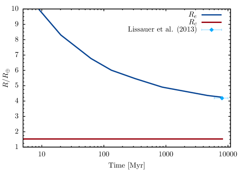
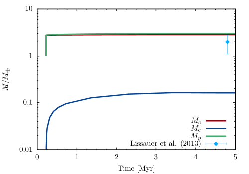
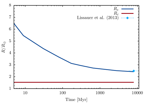
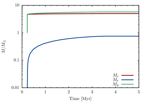
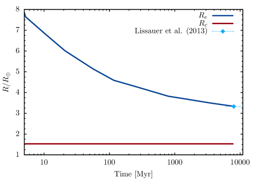
Table 2 gives a summary of the final properties of the six simulated Kepler 11 planets, along with the deduced value of . The final core mass, the final envelope mass, the final core radius, the final planet radius, the final planet luminosity, the composition, and the orbital position are presented.
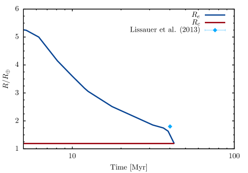
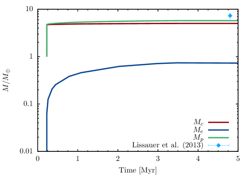
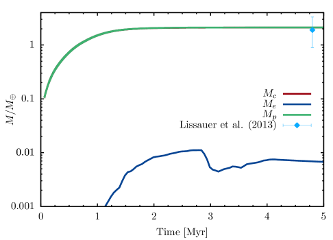
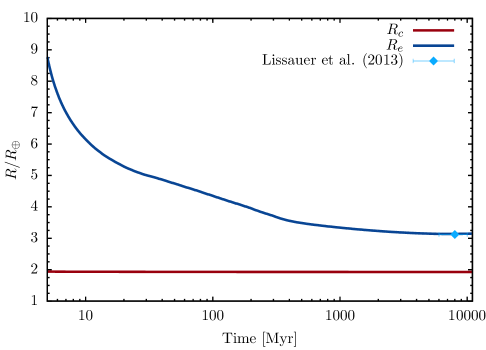
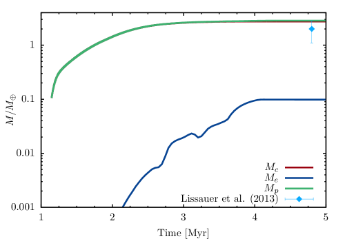
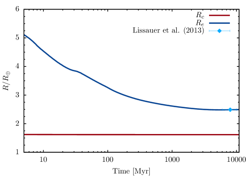
Figures 3 and 4 show, for the various planets, the evolution of the core mass, envelope mass, and outer radius. In general, because of the high solid surface densities required, the core mass increases rapidly, on a timescale years. In fact, by using Equation (6), the accretion timescale of the core is
| (24) |
where the cross section for planetesimals’ capture is when the gas bound to the core is very tenuous. If , Equation (24) gives initial accretion timescales (see and in Table 2) . Nonetheless, at an initial envelope mass of , even -size planetesimals are affected by gas drag in the envelope and becomes (D’Angelo et al., 2014). In the calculations, the actual timescales are all of the order of (see Figures 3 and 4). Thus, any uncertainties in Equation (6) or in the choice of the initial core mass have practically no effect on the final result. The core mass levels off at the isolation mass, as given by Equation (7). The envelope mass increases more slowly, on a timescale of . The outer radius during the formation phases shows an initial rapid rise corresponding to the rapid core growth, and then a nearly flat section since the outer boundary condition is essentially determined by the nearly constant core mass. Once the transition at is reached, the radius decreases rapidly as a result of the transition to isolated boundary conditions. Beyond that time, the radius decreases slowly as a result of contraction and cooling. As a further effect, the envelope mass and outer radius decline as a result of mass loss induced by stellar XUV radiation.
Some properties of the Kepler 11 planets at the time of disk dispersal (), according to our in situ models, are reported in Table 3. Planet Kepler 11b would lose its entire H+He envelope in years. For planets Kepler 11f through c, proceeding inwards, mass-loss rates are to at , decreasing to to at . At the final age of , these rates are down to to .
Specifically, the main results from our in situ models can be summarized as follows.
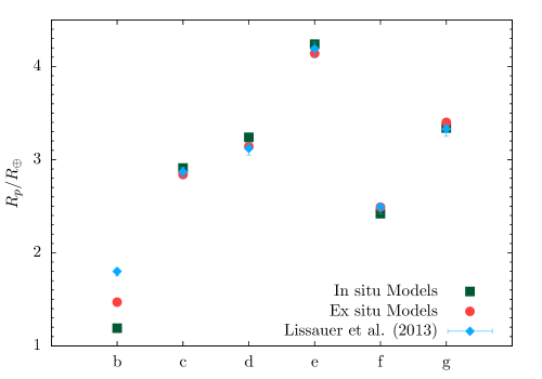
Kepler 11b. a low-mass H+He envelope forms around the core mass of , but during the isolation phase this envelope is entirely lost. The final mass is consistent with the measured mass (L13), but the final radius, the core radius of , is far below the measured value of , as shown in the top-right panel of Figure 3. Even by taking the upper limit of the measured mass, a % silicate core would still have too small a radius, only . A steam envelope (not modeled here) is probably required to achieve consistency (Lopez et al., 2012). This possibility, however, is inconsistent with in situ formation inside of a solar-type star because of the lack of ice in the core. Another possibility is the release of gas sequestered by the core during formation. The result that the entire envelope mass is lost remains valid even if the assumed core mass is increased to .
Kepler 11c. about half of the accreted envelope mass is lost during the isolation phase, but the final radius agrees with the measured radius of (see Figure 3, center-right). The final total mass of falls just above the one-standard-deviation upper limit for the measured mass of , but is certainly within the uncertainties in the theoretical models.
Kepler 11d. about one-third of the accreted envelope mass is lost during the isolation phase. The final computed radius of is within % of the measured value of (see Figure 3, bottom-right). The final computed total mass of is just below the one-standard-deviation lower limit for the measured mass of . These small discrepancies are well within the uncertainties of the models. To reduce the radius to agree with the measured value would require reducing the mass, increasing the discrepancy with the measured value.
Kepler 11e. at a separation from the star of about , the accreted H+He envelope of this object loses only about % of its mass during the isolation phase. The final computed radius of agrees to within % with the measured value of , as indicated the in top-right panel of Figure 4. The final computed total mass of agrees with the measured mass of . A slight reduction in the assumed mass (%) would bring the radius into agreement with the observed value and the planet mass would still agree with the observed mass, well within one-standard-deviation uncertainties.
Kepler 11f. even though the planet lies farther from the star () than Kepler 11e, its lower core mass ( vs ) results in % of the H+He envelope being lost during the isolation phase. The final computed radius of agrees with the measured value of to within % (see Figure 4, center-right). The final total mass of is slightly above the one-standard-deviation upper limit for the measured value of . To improve the agreement with the observed radius, the assumed mass would have to increase by about , increasing the (small) discrepancy with the observed value. In any case, the agreement is within the uncertainties of the theoretical model.
Kepler 11g. at a distance of , the planet loses only about % of its H+He envelope mass during the isolation phase. The computed final radius of agrees with the measured value of . The corresponding computed total mass is . The observed mass in this case is not well constrained; it is less than .
4. Ex Situ Formation Models
4.1. General Results

The two phases of planet evolution identified in Section 3 can also be defined in ex situ models. The time coincides with the time at which the disk evolution starts from the imposed initial conditions. The gaseous disk evolution depends on several quantities (see Section 2.4–2.6). The gas surface density at is with an exponential cut-off beyond some radius, so that a total disk mass of is initially confined within of the star (see, e.g., Williams & Cieza, 2011). This surface density distribution, , was determined after a number of attempts aimed at reproducing the observed physical properties of planet Kepler 11b and at tentatively matching those of Kepler 11f (the planet farthest from the star for which both and are constrained by transit observations). Only later it was realized that, fortuitously, inside matches quite closely the minimum-mass solar nebula density of Davis (2005). Although no other slope was tested for the initial , it is unlikely that the adopted initial surface density provides a unique solution to the problem. In any case, the choice of the initial density values is likely to influence the outcomes of the models more than does the choice of the initial slope .
These calculations apply a time-constant kinematic viscosity , where . In terms of the viscosity prescription of Shakura & Sunyaev (1973), the -parameter quantifying turbulence varies with time and distance from the star. The value around the starting orbital radius of the simulated planets is between and . The disk provides an initial accretion rate toward the star of order .
The lifetime of the gaseous disk is determined by , , the initial disk mass, and the photo-evaporation rate. All of these quantities are the same for all planet models. As mentioned in Section 2.6, the presence of a planet may affect disk dispersal, to a smaller or larger extent depending on the planet mass, its gas accretion rate, and orbital radius. In fact, although the planets end up inside the critical radius , they do spend most of their disk-embedded evolution at larger radii and, therefore, they can potentially influence . However, in the models presented here, this effect appears to be marginal and the gas inside is dispersed in , with a time-spread among models of about %.
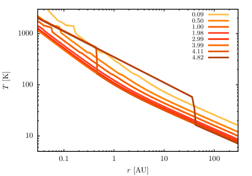
The evolution of and is illustrated in Figure 5 (see the figure’s caption for details). Dust opacity transitions are visible in the temperature profiles, the most prominent of which are represented by the evaporation of the silicate species above . The fainter opacity transitions associated with the evaporation of icy grains are also visible (located around at and at ). In the forming region of Kepler 11 planets (), the gas temperature is at and becomes at times . By the time the simulated planets have settled on their final orbits, the local gas temperature varies between and .
Gas photo-evaporation by stellar irradiation produces a density gap somewhat inward of , around the radius , where the ratio between the photo-evaporation timescale and the accretion timescale through the disk is smallest. Viscous diffusion quickly removes gas inward of on a timescale of (see Section 2.6), generating a cavity at . Afterwards, rim photo-evaporation dissipates gas inside-out, pushing the cavity edge outward to by (see Figure 5). Inside the disk cavity, which is virtually devoid of gas, the temperature is set equal to the irradiation temperature, so that . Beyond the cavity edge, the temperature is set by the gas thermal balance, Equation (12) (hence the large temperature transitions in the bottom panel of Figure 5 for ). The evolution of and in Figure 5 is the same for all models, except for variations induced by disk-planet tidal interactions and gas accretion on the planet.
| Planet | (Fe,Si,H2O)%bbPercentage of the core mass. ‘Fe’, ‘Si’, and ‘H2O’ indicate, respectively, the iron nucleus, the silicate mantle, and the H2O outer shell of the core (see Appendix A for details). | (Fe,Si,H2O,H+He)%ccPercentage of the planet mass. | [au] | [au] | |||||
|---|---|---|---|---|---|---|---|---|---|
| b | |||||||||
| c | |||||||||
| d | |||||||||
| e | |||||||||
| f | |||||||||
| g |

| Planet | [Myr] | (Fe,Si,H2O,H+He)%bbPercentage of the planet mass at time . | ccEquilibrium temperature of the planet, Equation (5), at . [] | ddRate of change of the planet’s envelope mass averaged over the first of evolution in isolation. For Kepler 11b, is an average over . [] | ||||
|---|---|---|---|---|---|---|---|---|
| b | ||||||||
| c | ||||||||
| d | ||||||||
| e | ||||||||
| f | ||||||||
| g |


The energy output of the central star can impact both the evolution of the disk and that of the planet. The two stellar models considered here (see Section 2.1) show similar luminosities for (see Figure 2), implying similar evolution of the planets in isolation. However, there are differences at earlier times, specifically in the effective temperature and radius , which enter the irradiation temperature in Equation (16). Therefore, the disk thermal budget may be affected and hence the planet migration history may differ somewhat (see Section 2.5). The temperature at the planet surface may also change. These differences are assessed for the cases of Kepler 11b and c (see Section 4.2).
Among the main simplifications of this study are the neglect of planet-planet interactions and the fact that only a single planet evolves in the disk, though the models account for the depletion of the planetesimal disk generated by planets that have already initiated the formation process. It is assumed that by the time , a solid core of mass (corresponding to , calculated consistently with and the disk boundary conditions) has formed at a current orbital radius of . There is no speculation about its previous accretion/migration history and is considered to be the initial orbital radius of the simulated planet. (However, the small initial planet mass implies that orbital migration via disk-planet tidal interactions may be negligible at times ). Both and are free parameters, constrained by the requirement, among others, that no two orbital paths intersect each other. Strictly speaking, this is not a physical requirement (e.g., Hands et al., 2014) but rather a necessity dictated by the absence of gravitational interactions among planets. The time ranges from (Kepler 11b) to (Kepler 11f). Clearly, the time is also determined by the choice of using the same initial core mass for all planets. The orbital radius ranges from for Kepler 11f to for Kepler 11e.
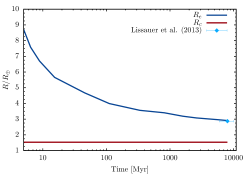
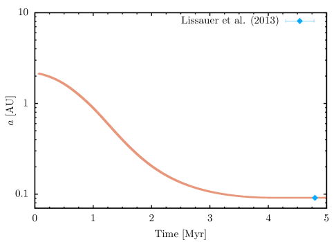
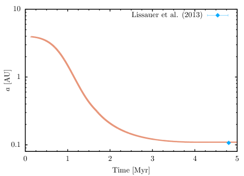
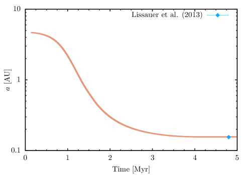
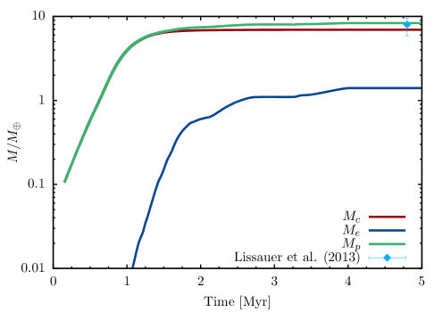
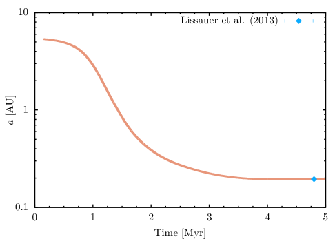
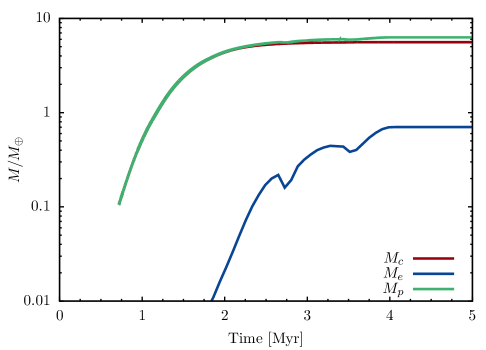
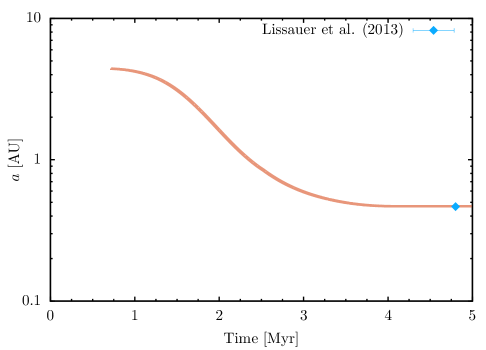
Table 4 summarizes the final properties (and ) of the six simulated Kepler 11 planets, assumed to have formed ex situ. These are referred to as reference models. The initial orbital radius of each planet, , and the epoch are found by trial and error so that the final model provides reasonable matches to , , and at an age of , as reported by L13. Additionally, as mentioned above, orbital paths must not intersect. Plots of various quantities versus time from the resulting models are illustrated in Figures 6 and 7. Since all planets start well beyond , contrary to in situ models, the local density of solids at and is moderate to low: for Kepler 11b, for Kepler 11f, and between and for the other planets (in ascending order of ).
Models for each planet were constructed in ascending order of final orbital radius, . At time , the gas-to-solid mass ratio is set to about beyond the ice condensation line at around (). Planetesimals are anhydrous interior to (), where the gas-to-solid mass ratio becomes approximately (see Section 2.2 for details). As the disk evolves, the ice sublimation line moves inward to by (see Figure 5). The model for Kepler 11b is constructed from this initial surface density of solids, . The distribution is depleted by the passage of Kepler 11b. Indicating with the initial and the final (i.e., observed) orbital radii of Kepler 11c, the distribution for modeling this planet is determined by taking the depleted mass in solids between and , and redistributing the mass over the region according to a power law. The same procedure is used to determine for the construction of models for Kepler 11d and e (each based on the depleted reservoir of solids left by the preceding planet). For the models of Kepler 11f and g, which start inside the orbits of preceding planets at significantly later times, the depleted mass in solids is redistributed interior to (down to their observed orbital radii).
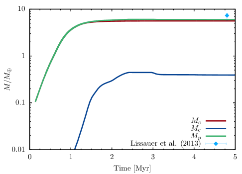
Typically, models make a transition from disk to photospheric boundary conditions (see Section 2.1) at the isolation time, . Although in some models gas accretion can be disk-limited during late stages of formation, as for in situ models a proper phase of rapid gas accretion (i.e., significantly smaller than ) is never reached during the formation phase. Accretion of solids could in principle (and does on occasion) continue beyond the isolation time, until the feeding zone is emptied (which requires ). However, since orbital migration becomes very slow much earlier than (see Figures 6 and 7), plateaus well before isolation is achieved, as can be seen in the left panels of Figures 6 and 7. For all practical purposes, a planet is isolated from both the disk’s gas and solids at . Some properties of the reference models of Kepler 11 planets at are listed in Table 5. The small scatter in isolation times is likely caused by the removal of gas via accretion on the planet (when ), which tends to lower the accretion rate through the disk for (Lubow & D’Angelo, 2006, see also Equation (11)) and thus operates in concert with disk photo-evaporation to augment gas depletion inside . In fact, the time is shorter for planets with larger envelope masses, i.e., with larger . However, the contribution of to is quite marginal in these calculations. In the more realistic situation in which all planets migrated in the disk, the time would be set by the largest planet, Kepler 11e. However, since the formation phases of all planets are basically complete by that time, no significant consequences would be anticipated.
The relative gas content is largest for Kepler 11e, accounting for % of the total mass at , and somewhat less at (see Table 4). The light elements (H+He) in the other planets make % of the total mass at the isolation time and, in most cases, only a few to several percent at . At this age, however, the gaseous envelope always accounts for % to % of the planet radius. For all planets, the condensible mass fraction of H2O is %, indicating that their cores mostly form behind the ice condensation line. Although the composition of the initial core is dictated by the local disk composition of the solids at , its mass () is small enough to not affect the final core composition much. Kepler 11b contains the smallest mass fraction of H2O and the largest mass fractions of silicates and iron, due to its small initial orbital radius () and early start time, . Nonetheless, also in this case the substantial fraction of H2O (% by mass) implies that the planet accumulates its condensible inventory mostly behind the ice condensation front. Despite an equally small starting orbit, the core composition of Kepler 11f is instead more similar to that of neighboring planets because of its late start time () and growth in a colder disk environment.
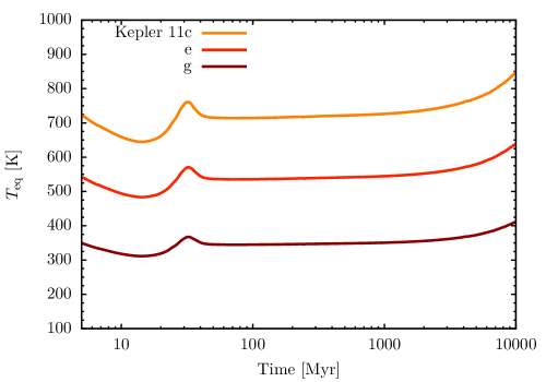
Except for the varying stellar properties (see Figure 2), the isolation evolution of ex situ models behaves as that of in situ models. The surface temperature of the planet closely follows the equilibrium temperature, , which is shown in Figure 8 for the isolation evolution of Kepler 11c, e, and g.
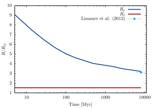
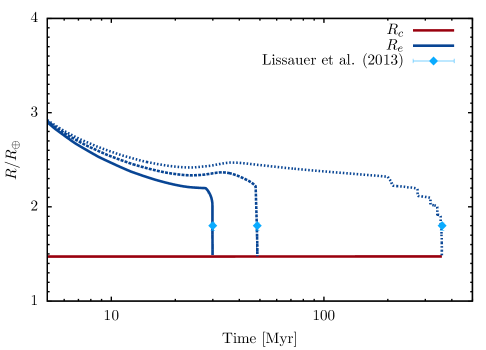
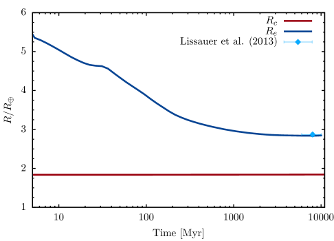
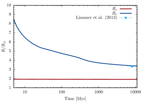
As for in situ models, the planet radius decreases on a short timescale once the planet becomes isolated. Afterwards, steadily declines as the planet cools. The radius of planets Kepler 11c and d reaches a minimum at an age between and , after which the envelope begins to slowly expand, following the rise of (see Figure 8). However, the expansion is very modest and by an age of , increases over its minimum value by %. Kepler 11f follows a similar trend, achieving a minimum radius around the age of and then inflating slightly ( changing by %). Possibly due to their more massive envelopes and hence larger internal energy, the simulated planets Kepler 11e and g still contract at an age of .
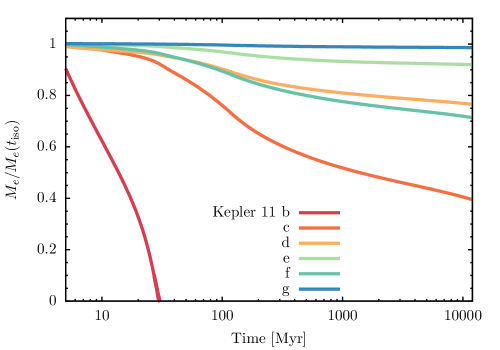
The evaporative loss of envelope gas, caused by the absorption of stellar X-ray and EUV photons and given by Equation (8), starts at , i.e., as soon as the gaseous disk interior to the planets’ orbit is cleared and the isolation phase begins. As for in situ models, a standard value for the efficiency parameter, , is applied (but see also Section 4.2). The resulting envelope masses versus time are illustrated in Figure 9. The rate is especially large at early ages, , because both and the flux (see Section 2.3) are large. Values of the gas loss rates, averaged over the first ( for Kepler 11b) of evolution, are listed in Table 5 and range from to around , i.e., between and . Mass loss is significant for the inner planets Kepler 11b, c, and d. By these planets lose, respectively, %, %, and % of their at . Envelope loss is also substantial for Kepler 11f, which loses nearly % of its gaseous mass during the isolation phase. In relative terms, Kepler 11e and g are more immune to evaporative mass loss, as reduces by about % and %, respectively, from to . Of the H+He mass removed during isolation, at least –% evaporates within . As planets contract, hence in Equation (8), and H+He gas is stripped from the envelope at a rate . After , mass-loss rates become quite small for all planets, ranging from around (for Kepler 11f and g) to (for Kepler 11c and d).
Comparing the evolution of in Figures 3 and 6 after isolation, one can see that planets formed in situ remain somewhat more inflated than do planets formed ex situ. The difference is especially large for the case of Kepler 11b, probably due to the fact that the planet formed in situ acquires a more massive H+He envelope (because of the rapid core growth). Differences tend to vanish at later times. This behavior accounts for the differences in the average rates in Tables 3 and 5. Although there is a factor of difference in the gas loss rates between in situ and ex situ models of Kepler 11b, in this case, the difference is immaterial since both simulated planets lose their entire envelopes within –.
4.2. Results for Individual Planets
The main results from our ex situ reference models can be summarized as follows.
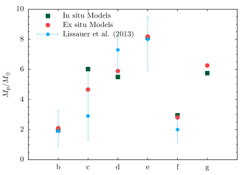
Kepler 11b. at an initial orbital distance of () and a surface density of solids , according to Equation (7) a non-migrating core would achieve a final mass of , and smaller if depletion via scattering (Equation (18)) was taken into account. About % of the core mass is accreted from solids orbiting beyond from the star, hence the presence of large amounts of H2O in the planet. The envelope mass is maximum around , before part of it becomes unbound and is released back to the disk. After the planet becomes isolated, the remaining H+He gas is removed by stellar X-ray and EUV radiation within . Reducing the efficiency of the evaporative mass-loss rate, in Equation (8), allows the planet to retain an atmosphere for somewhat longer. However, even a value as low as predicts a complete removal of the primordial H+He gas within a few times (see Figure 6). Despite the presence of abundant H2O in the core (% by mass), is still significantly smaller than the observed radius. Although not included, this model naturally accounts for the formation of a steam atmosphere that was proposed to reconcile simulated and observed radii (Lopez et al., 2012). Both final orbital radius and planet mass agree with measured values (see Figure 10).
Kepler 11c. the planet starts at roughly () and grows about % of its condensible final mass at . Nearly % of the planet’s final mass is in H2O, the second largest (after Kepler 11f) relative fraction of all simulated planets (although Kepler 11d, e, and g contain more H2O in absolute measure). When the local disk disperses and the planet becomes isolated, the envelope includes about % of . Roughly % of this H+He mass is accreted from the disk’s gas at . Over the course of the isolation phase, stellar radiation removes more than half of the envelope mass, leaving only % of in primordial H+He gas at , the smallest relative fraction in all simulated planets that retain an envelope. The evolution of in Figure 6 shows a period, between and , in which the planet contraction slows down. This feature is likely associated with the rise in at that age (see Figure 8), following the brightening of the star (Figure 2). A similar feature appears in the radius evolution of Kepler 11b and f planets, which can more promptly respond to changes in the external incident flux having (with Kepler 11c) the least massive envelopes. The final planet mass and radius agree with measurements, whereas the final orbital distance is just above the one-standard-deviation upper limit of the measured value ().
Kepler 11d. the starting orbital radius is less than larger than that of Kepler 11c and the start time is comparable (). Therefore, similarly to its inner neighbor, the planet accumulates % of outside of . The maximum value of is attained shortly prior to , but afterwards some envelope gas becomes unbound and returns to the disk. For prior to isolation, remains very close to the accretion radius , preventing further accretion of gas. During its evolution in isolation, the envelope loses somewhat less than , about a fifth of at . Comparing the core radii in Tables 4 and 5, a small difference can be noticed. The core masses at and at are virtually identical, yet the pressure applied at the top of the core at the later epoch is nearly twice as large ( vs. ) because of the cooler temperature, which in this case accounts for the reduction in . The values of the planet’s mass and radius and the orbital distance at are all within measurement errors.
Kepler 11e. the most massive of the six, in terms of both core and envelope mass, this planet also has the farthest initial orbit at () from the star. The initial local density of solids is . Neglecting scattering, a non-migrating planet at that distance would achieve a final core mass of around before emptying its feeding zone. The planet grows % of its core mass beyond , but most of its H+He inventory is accreted inside this radius. Essentially, the planet’s core fully forms behind the ice condensation line (% of is H2O). The average mass-loss rate at the beginning of the isolation phase (, see Table 5) is higher than that of Kepler 11d despite the larger mass and orbital radius of Kepler 11e. The reason is the strong dependence of in Equation (8) on planet radius. In the case of Kepler 11d, drops below by , whereas the radius of Kepler 11e remains well after (see Figure 7). In absolute terms, the planet loses the second largest amount of primordial H+He during the isolation phase (). The difference in between and is again caused by the pressure difference at the bottom of the envelope. The final values of , , and all agree with measurements.
Kepler 11f. the observed mass of the planet is significantly smaller than those of its neighbors, possibly suggesting a formation at a smaller orbital distance. To achieve a correspondingly smaller core mass with our , the planet’s initial orbit is interior to the initial orbits of the other planets. Consequently, the planet requires a late start, , to avoid crossing other orbital paths111 This solution is unlikely unique, and an earlier start may be possible together with a wider initial orbit and a lower . In this case, however, the slower growth of would entail larger gas densities to account for the required amount of orbital migration.. The assembly of the core takes place for the most part beyond and at disk temperatures of . As a result, the core composition is very similar to that of fully hydrated planetesimals (% H2O and % silicates by mass). Though rich in H2O in relative terms, % of (the richest, in fact), because of its small mass the planet contains an amount of H2O () greater only than the H2O mass of Kepler 11b. During the evolution in isolation, stellar radiation strips off about % of the H+He gas accreted during the formation phase. At , the planet is left with a gas content of % by mass. The final planet radius and orbital distance agree with observations, whereas the final total mass, , is close to the one-standard-deviation upper limit of the measured value ().
Kepler 11g. similarly to its inner neighbor, the planet starts its simulated evolution at an advanced stage of the disk’s life () in between the initial orbits of Kepler 11c and d. Roughly % of its condensible inventory is collected beyond , and all of the core is accumulated behind the ice condensation front. In fact, its formation occurs at disk temperatures below and its core has virtually the same composition as that of fully hydrated planetesimals. Partially hydrated planetesimals account for only % of the core mass. Mass loss during isolation is negligible, and the planet basically contracts at a constant mass. Again, the core shrinks somewhat as the envelope cools down and the applied pressure at increases. The planet radius at is just above the one-standard-deviation upper limit of the measured value (), whereas agrees with measurements. The planet mass is not really constrained by transit observations, but the value provided by this ex situ model is consistent with that from the in situ calculations in Table 2. Both simulations point at a planet somewhat less massive than Kepler 11e and of comparable mass to that of Kepler 11d.
4.3. Effects of Changes in Model Assumptions
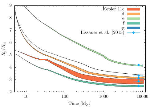
The reference models use a standard value of in the expression of , to account for re-radiation of the EUV and X-ray stellar flux by the envelope (see Section 2.3). Since this parameter is uncertain, the evolution in isolation was repeated by applying values of and . Results for the evolution of are plotted in Figure 11. The case of Kepler 11b is omitted for obvious reasons. The solid curves of each pair (upper curve for the smaller efficiency) bracket the excursion of (colored regions). Within the considered range of , the impact on the radius at is typically small. For Kepler 11g and e, the relative excursion of amounts to about % and %, respectively, and the percentile variations of are % and %. The excursion of is larger for Kepler 11d (%) and larger still for Kepler 11f (%), owing to its small mass. The relative change in , though, is % for either. In all these cases, the simulated planets would still provide reasonable matches to the observed planets, with and lying within or proximate to measurement ranges. Due to its vulnerability to mass loss, Kepler 11c represents the most extreme case, with changing by a factor of three and by %, which would place the planet radius well outside of the measurement range.
The reference models are based on time-dependent stellar properties for a ([Fe/H]) star computed by Siess et al. (2000). In order to determine the impact of the stellar evolution model, which enters the calculations through Equations (5), (8), and (16), a simulation of Kepler 11b was performed with the Yonsei-Yale stellar model (Spada et al., 2013) in Figure 2 (see the figure’s caption and Section 2.1 for further details), starting from the same disk’s initial conditions as in the reference model. The three equations depend on (, although Equation (16) separately depends on as well). The largest differences in stellar luminosity between the two stellar models occur for , i.e., during the disk-embedded phase and the early isolation phase of the planet. The Yonsei-Yale stellar model predicts lower luminosities, which tend to produce a somewhat cooler disk in regions where stellar irradiation is important in the energy budget of the gas (Equation (12)). The cooler temperature in turn reduces the disk thickness and hence affects the migration rate, since (see Equation (22)). The cooler temperatures during the nebular stage of the planet’s evolution also change the Bondi radius , and hence the planet accretion radius in Equation (1). By using the same initial orbital radius, , as in the reference model (see Table 4), the somewhat larger (in magnitude) migration speed requires a later start time, (the difference in luminosity is especially large for , see Figure 2). The resulting model provides an isolation time of and values at in very good agreement with those in Table 5. During the isolation phase, the surface temperature of the planet differs by relative to that of the reference model. The H+He envelope is entirely removed by , as in Figure 6. Because of the cooler gas temperatures and later start, the core contains a slightly larger H2O fraction (% vs. % by mass).
Since the isolation phase of Kepler 11b does not last long, a calculation with the Yonsei-Yale stellar model was also performed for the isolation phase of Kepler 11c. The properties of the model at are those of the reference model listed in Table 5. For most of the isolation phase (), the stellar luminosity of the Yonsei-Yale stellar model is around % lower, compared to of the Siess et al. model, and thus is only marginally different. The calculation results in an envelope mass at of and a planet radius of . Both numbers are a little larger than the values in Table 4, but within the errors of the measured mass and radius of Kepler 11c. Clearly, the stellar evolution model does not affect the simulated planets significantly.
Dust grains, either entrained in the accreted gas and/or produced by ablation of accreted solids, can pollute planetary envelopes at temperature (assuming silicate grains). In such cases, dust opacity regulates the envelope cooling rate and hence the planet’s contraction timescale (e.g., Pollack et al., 1996; Hubickyj et al., 2005). The calculations presented here are based on the opacity plotted in the top panel of Figure 1, which assumes a maximum grain radius of . To evaluate the effect of grain opacity in the envelope of the reference models, calculations were also performed by using the table plotted in the bottom panel of Figure 1, which assumes a maximum grain radius of . The ratio of the grain-dominated, Rosseland mean opacities in the two tables is about eight. The lower opacity provided by the size distribution with larger dust grains is expected to facilitate cooling and allow for higher gas accretion rates. The planet Kepler 11b, which accumulates the least massive H+He envelope, was simulated with the lower grain opacity. By using the same initial conditions for both disk and planet as for the reference model, the calculation provides values of that are initially a few times as large as those of the reference model. The envelope mass achieves a maximum value of at a time , after which the envelope loses mass to the disk as tends to exceed the accretion radius . The planet attains isolation at a time . Despite the larger envelope mass during the planet’s early accretion history, the core mass at is again and (about twice as large as that of the reference model), which is entirely removed by stellar radiation by an age of .
Although the opacity test indicates little impact on the simulated Kepler 11b planet, larger effects are to be expected for planets that accumulate higher H+He mass fractions. Indeed, the same test repeated for the most massive planet, Kepler 11e, results in an entirely different outcome. The planet reaches a crossover mass () of at and enters the transition stage (see Section 2.1) of fast – and disk-limited – gas accretion by . On its track to becoming a Hot Jupiter, the planet reaches a mass of by . The tendency to evolve into a giant planet, with the lower dust opacity of Figure 1 (bottom panel), is also obtained from in situ calculations. Ex situ models matching the observed radius of Kepler 11e with the lower opacity require a smaller core mass and, hence, a tighter initial orbit (). A calculation resulting in at provides a mass , below the one-standard-deviation lower limit of the measured value of . A calculation resulting in produces a radius , well over the one-standard-deviation upper limit of the measured value of . Similarly, in situ formation models indicate that can be matched with a mass somewhat smaller than the measured one-standard-deviation lower limit.
Both in situ and ex situ models assume formation in a disk of -radius planetesimals. A reduction in planetesimal size from to was studied by the authors in other contexts. First, the orbital eccentricities and inclinations of these bodies decrease, and second, the cross section for planetesimal capture in the planetary envelope ( in Equation (6)) increases (see D’Angelo et al., 2014, Figure 6). Both effects enhance the accretion rate of solids, . Whether the planetesimal size has an effect on the accreted gas mass depends on the ratio of the timescale for the buildup of the core to the disk lifetime. The core buildup timescale of the in situ models is already very short, thus the effect is negligible. In the ex situ models, the core accretion time would decrease (considerably in the case of small planetesimals). The faster core growth would increase the migration rate. The planet would be driven more quickly toward the inner disk regions, where solids’ densities are higher but the solids’ mass available for accretion is lower. Therefore, the outcome is difficult to predict. We performed tests for Kepler 11d with planetesimals of and in radius. Compared to the reference case discussed above, the final core mass increased by only about % and %, respectively.
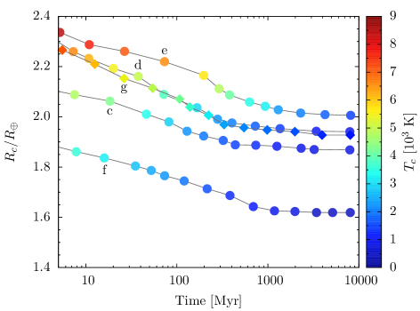
The data listed in Tables 4 and 5 indicate that there can be marginal changes in core radii during the isolation phase. As mentioned in Section 4.2, these changes arise from differences in boundary pressures caused by contraction, resulting in core compression. Such small changes, however, may be offset by temperature effects through the core. In the calculations discussed above, core thermodynamics is ignored and ex situ models include it only for phase transitions within the silicate mantle (see Section 2.2 and Appendix A). The assumption of neglecting the core thermal stratification is based on previous studies, which argued that thermal pressure should not significantly affect the core radius at these core masses (e.g., Valencia et al., 2006; Seager et al., 2007; Sotin et al., 2007; Sohl et al., 2014b). Nonetheless, for completeness, improved structure models are presented and discussed in Appendix C. These include temperature stratification, energy transfer, and temperature-dependent EoS in a self-consistent fashion; they also include additional material phases. Thermal effects (in H2O-rich cores) may be relatively important for the determination of during the early stages of the isolation phase (, see Figure 12). However, at an age of , the differences in between thermal and isothermal cores of the simulated Kepler 11 planets are small, typically % in most cases and somewhat less than % for Kepler 11c. Assessing the impact of thermodynamics for the case of Kepler 11b is more difficult, because the expected steam envelope is not modeled. If the gas pressure and temperature at the bottom of the envelope were, respectively and , then would be % larger than the value listed in Table 4 (see the discussion in Appendix C).
During isolation, planets gradually cool down. The pressure at the bottom of the envelope varies by factors of the order of unity, whereas temperature variations are larger. To make a simple assessment of the impact on of the varying conditions at the core-envelope boundary as planets cool, thermal structure calculations of the cores (see details in Appendix A) were performed by applying pressure and temperature at the core surface during the isolation phase. Figure 12 indicates that there can be significant variations in , up to . The symbols in the figure are color-coded according to the core surface temperature, , as obtained from ex situ calculations. However, in the figure, –% of the total difference along each curve is due to the contraction of the cores’ H2O shell. Additional details are given in Appendix C. Assuming , the inflated cores may result in planet radii larger by % at around the isolation time, which may in turn enhance the evaporative mass-loss rate by % during early isolation times. Results in Figure 11 suggest that the impact on at may be relatively small.
4.4. Effects of Changes in Initial Conditions
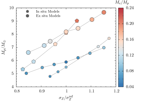

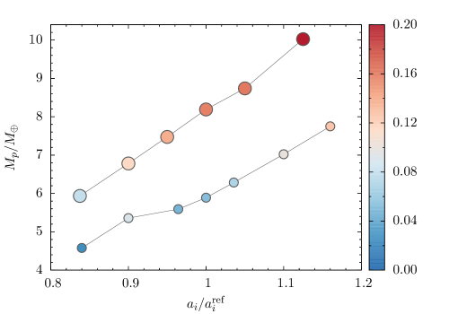
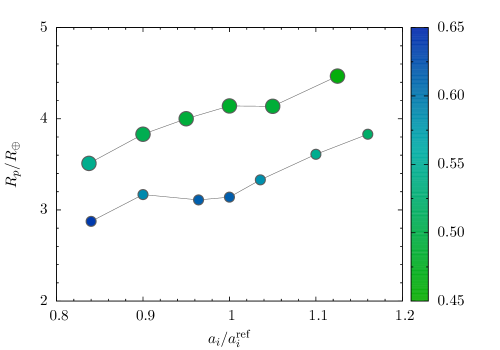
Figure 13 illustrates how some properties of the models for Kepler 11d and e at depend on the surface density of solids, , and the initial orbital radius, (see the figure’s caption for further details). Where relevant, in situ models are included as well. In the figure, and are the reference values of the models discussed in Sections 3 and 4. In the calculations of the top panel, the initial gas density is rescaled so to keep the ratio fixed. The planet mass increases monotonically as and increase. In either case, this is a consequence of the larger core mass that facilitates gas accretion, especially at early times. The final envelope mass of in situ models increases monotonically, as it generally (but not always) does also in ex situ models. In the latter calculations, because of the different accretion history (and initial condition ), the final orbital radius varies, affecting the evolution of during isolation. The radius tends to grow with the ratio , which is not always a monotonic function of or in ex situ models (see the left panels of Figure 13). Because of the small uncertainties on the observed radius, only initial conditions in the neighborhood of those adopted for the reference models can match observations. The final orbital distance varies by a factor of up to in the ex situ calculations of the top panels and in those of the bottom panels (relative to the reference values, and ).
The in situ reference models of Section 3 and those represented in Figure 13 assume an initial disk’s gas-to-solid mass ratio of . Experiments conducted on Kepler 11e, by using (as in the reference case) and varying the mass ratio from to , resulted in mass and radius changes (at ) of %. For a gas-to-solid mass ratio of , and whereas these values increase to and , respectively, for a mass ratio of . The planet mass is still within measurement errors, while the planet radius lies outside the observed range by at most a few percent.
5. Discussion
5.1. Implications of In Situ and Ex Situ Formation

Both in situ and ex situ simulated planets result in radii, masses, and orbital distances in agreement with measured values at the estimated age of the system. Therefore, it is not possible to distinguish between the two modes of formation from these final properties. The two formation scenarios do, however, provide entirely different perspectives of the environment in which the planets grew, of their compositions, and interior structures.
Figure 14 shows the initial surface density of the gas applied to the in situ (circles) and ex situ models (blue line). The figure also illustrates other reference surface densities (Weidenschilling, 1977; Hayashi, 1981; Davis, 2005; Chiang & Laughlin, 2013; Schlichting, 2014). As noted above, at of the ex situ simulations fortuitously matches the surface density constructed by Davis (2005). It should be pointed out that, among these reference density distributions, only those of Chiang & Laughlin (2013) and Schlichting (2014) were explicitly derived for close-in extrasolar planets. The other two are meant to apply to the solar system and are thus simple extrapolations at the short distances from the star of Kepler 11 planets. The dashed line in the figure indicates the gas density above which the disk would be gravitationally unstable to axisymmetric perturbations according to the Toomre stability criterion (Durisen et al., 2007, pp. 607-622), using a constant gas temperature of . Even by applying , appropriate for nearly constant, the initial inferred from in situ models would still be stable (although only marginally stable to non-axisymmetric perturbations).
In situ formation requires a very large within of the star, as illustrated in Figure 14 (see also Bodenheimer & Lissauer, 2014). The models discussed here suggest densities of solids between and (see Table 2). If most of these solids had to form locally, the initial gaseous mass of the region had to be accordingly large. Given the short accretion timescales involved in the growth process, (see Figures 3 and 4), most of the solids necessary for core assembly had to be available prior to the beginning of this process. Therefore, a gradual replenishment of the solids’ reservoir from larger radii might not be a viable alternative to a large . Moreover, this possibility would likely lead to a hierarchical system of planets with inwardly decreasing masses, which is inconsistent with the masses of Kepler 11f and e (and probably of Kepler 11g as well).
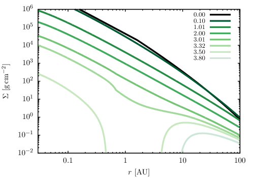
A disk model aimed at mimicking the evolution of the initial in situ shown in Figure 14 is presented in Figure 15. The disk has an initial mass of within . Both the kinematic viscosity of the gas and the emission rate of stellar EUV ionizing photons were chosen to induce photo-evaporation of the inner disk at around the age of (see Section 3). The region in the disk in Figure 15 is dispersed between and . Gas temperatures are initially high, as can also be realized from simple arguments based on energy balance. At high densities, the disk is optically thick in the vertical direction and the main source of energy is viscous heating. Hence Equation (12) reduces to , which becomes
| (25) |
where is the optical depth of the disk’s mid-plane. Since the initial accretion rate through the disk in this case is , Equation (25) and Figure 15 imply that, at , temperatures are initially in excess of and drop below at . At , temperatures become at . These high gas temperatures would only allow for the presence in the disk of metals and highly refractory solid species, which would be reflected by the compositions of the cores. The high temperatures also prevent the massive inner disk from becoming gravitationally unstable (Durisen et al., 2007, pp. 607-622). Lowering the kinematic viscosity of the gas would somewhat reduce the gas temperatures () but would also extend the disk lifetime (by halving it would take over to photo-evaporate the inner disk). The effects of the initially high disk temperature and of the disk evolution on the in situ formation process require further calculations.
Ex situ formation can occur in low-mass disks, in which the initial increases from at around to at , the disk region that provides the vast majority of the solids to assemble all the planetary cores. Initial gas densities at these radial distances are in the range from a few times to (see Figure 5). Cores are assembled over timescales of the order of (see Figures 6 and 7). Planets experience relatively low temperatures during their formation phase and spend a long enough time behind the ice condensation line to become enriched in H2O and other volatile substances (if available).
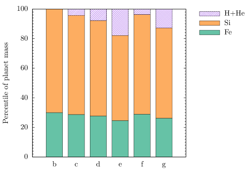
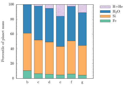
The percentile composition of the six planets is represented in the histograms of Figure 16, for in situ as well as ex situ models (see the figure’s caption for details). Recall that in situ simulations assume a fixed core composition of iron and silicates of % and % by mass, respectively. In ex situ models, H2O is assumed to be all condensed in the core, although part of it should be in gaseous form mixed with H+He gas, released by ablating solids passing through the envelope. Both in situ and ex situ calculations predict that the percentile H+He mass of Kepler 11c is comparable to that of the smaller Kepler 11f, because most of the envelope is lost after formation. Kepler 11b simulated in situ acquires a much larger envelope than does the ex situ simulated planet, because the core mass approaches its final value at very early times (compare the growth of in Figures 3 and 6).
In order to reconcile observed and simulated radii of Kepler 11b, the in situ formation scenario requires that gas is sequestered in the core during formation and released afterwards. Outgassing of at least of hydrogen would be sufficient to account for the observed radius. However, outgassing would still need to compete against evaporative gas loss, which would operate at rates between and . If outgassing began right after the removal of the primordial H+He envelope (at ) and continued for the age of the planet, the (average) outgassing rate would only need to be marginally higher than the (average) evaporative gas loss rate. This possibility, however, implies that the amount of gas sequestered in the core during formation ought to be significant in relative terms, between and . The details regarding the processes of sequestration and outgassing remain to be investigated, but the result could have important implications concerning the in situ versus ex situ formation of Kepler 11b.
The ex situ formation scenario predicts the presence of a steam atmosphere (not modeled here). Based on previous assessments of the planet mass and radius (Lissauer et al., 2011a), Lopez et al. (2012) estimated that the planet radius can be matched by a water-world whose composition is about % H2O by mass, comparable to the H2O content of the simulated ex situ planet (see Table 4). Assuming a hydrostatic and adiabatic atmosphere with an ideal EOS for H2O, the mass necessary to match the observed radius is , though non-ideal effects in the EOS may reduce this estimate. Because of the larger mean molecular weight, evaporative mass loss of H2O by stellar radiation should be less significant than is loss of lighter elements. Additionally, steam can be replenished by the condensed core. Since hydrogen can mix with H2O at the pressures and temperatures of planetary interiors (Soubiran & Militzer, 2015), hydrogen may be present in the atmosphere of Kepler 11b as well.
5.2. On the Mass of Kepler 11g
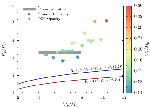
Transit observations only place an upper limit of on the mass of Kepler 11g (L13). Assuming negligible amounts of gas in the envelope, an ex situ type composition of % iron, % silicates, and % H2O by mass, would result in a radius of , short of the observed value . An in situ type composition would result in an even smaller radius (). Hence, the planet must bear a gaseous envelope.
Both in situ and ex situ models indicate that Kepler 11g is somewhat less massive than Kepler 11e and of comparable mass to Kepler 11d. It is reasonable to imagine a scenario in which a lower core mass may attract a sufficiently large envelope to account for the observed radius. In fact, another simulation of Kepler 11g (with different start conditions) results in a radius only marginally smaller than that observed and . Even smaller masses might be attained, e.g., by lowering the dust opacity in the planet’s envelope. However, the opposite scenario of a much more massive planet and a smaller ratio may be more difficult to realize.
Figure 17 shows outcomes from additional ex situ simulations of Kepler 11g. In these models, the start conditions of the reference model (, , and initial ) were changed with the aim of obtaining different planet masses and gas-to-condensible mass ratios. The final orbital radii are within roughly % of the observed orbital distance. Circles represent simulations that apply the grain opacity of the top panel of Figure 1, as in reference models. Data points are color-coded by their relative gas content, . The solid lines indicate the core radius corresponding to the interior composition of in situ (% iron and % silicates) and ex situ models (see Table 4), assuming a pressure at of and . The observed radius of the planet, within measurement errors, is indicated by the gray-shaded area. The data points include the in situ simulation of Table 2 as well. This model has a comparatively large gas content for its radius, owing to the smaller value of (i.e., the difference is in fact comparably large).
From the data plotted in Figure 17, it appears difficult to reconcile observed and simulated radii for planets more massive than about . In fact, when , the H+He mass fraction tends to exceed %, resulting in too large a radius. In the calculations reported herein, the value of at the end of the formation phase is set by dispersal of the gaseous disk. The model with largest mass in Figure 17 has () and far larger than observed. If under different circumstances the accretion of gas was starved by disk dispersal at an earlier age and at was similar to the observed value, the planet mass would not exceed (an envelope mass somewhat smaller than appears necessary to account for the observed radius).
According to L13, an planet with a % gas content by mass can match the radius of Kepler 11g. It may be possible to build a large core mass without attracting an excessively large envelope by augmenting the opacity in the envelope, which operates to slow contraction and inhibits gas accretion. This possibility was tested by using dust opacities calculated from an interstellar medium-type grain distribution, with dust grains of up to in radius (for details, see D’Angelo & Bodenheimer, 2013). Results from this second set of models are represented by diamonds in Figure 17. As expected, for a given , the ratio is smaller than in the other set of simulations, yielding smaller planetary radii. Nonetheless, as grows beyond , and becomes too large to match observations. Clearly, other scenarios can be envisaged (e.g., most of is accumulated toward the end of the disk lifetime, delaying envelope growth), although they must be compatible with the formation of the inner planets. Within the assumptions adopted herein, both in situ and ex situ models argue in favor of a mass smaller than or comparable to Kepler 11e’s mass.
6. Conclusions
We constructed models of formation and long-term evolution of the six Kepler 11 planets. Both in situ and ex situ scenarios were considered. The simulations presented here take into account many physical aspects of the formation and evolution processes in detail (see Section 2). Approximations were nonetheless necessary in order to render the problem tractable. A major limitation of this study is the neglect of planet-planet interactions. Although it is not possible to speculate about the impact of this deficiency on the results, especially in regard to orbital stability of planets and capture into mean-motion resonances, N-body simulations did show that compact planetary systems, and the Kepler 11 system in particular, may indeed originate in the presence of disk-driven orbital migration (Hands et al., 2014).
Both in situ and ex situ models appear equally capable of generating planets whose radii, masses, and orbital distances (when relevant) at the estimated age of agree with those measured via transit observations (see Sections 3 and 4). Based exclusively on these final outcomes of the simulations, it seems difficult – and certainly not obvious – to argue in favor of one scenario over the other. The implications of the two formation scenarios are, however, significantly and profoundly different (see Section 5).
In situ formation may only work if a large amount of solids is available for accretion within of the star. The models built here predict a surface density of solids (see Table 2) and a mass in solids of inside . Initial gas densities in the disk are expected to be accordingly high (, see Figure 15). Planets form at disk temperatures of over , hence their cores may only contain metals and refractory materials. The large values of also result in extremely short assembly times of the cores (of the order of , see Figures 3 and 4). Kepler 11b, which is completely stripped of its primordial H+He envelope during the isolation phase (a fate that appears unavoidable!), must have a tenuous atmosphere continuously replenished over time, or generated at a late age, by the release of gas sequestered in the core. More detailed modeling is required, taking into account the release of hydrogen as well as the evaporation of the atmosphere, to determine if this picture is reasonable.
Ex situ formation may work in low-mass disks. The models built here are based on a disk whose distribution of solids at is , proceeding inward from to . The initial gas density in this region ranges from to (see Figure 5). The disk’s gas interior to is dispersed in about . Cores grow gradually, over timescales of the order of (see Figures 6 and 7). In all cases, most of the core assembly may be completed beyond the ice condensation line (). Consequently, ex situ formation predicts planetary cores to be rich in H2O, and possibly in other volatile materials, if hydrated planetesimals bear substantial amounts of ice (as assumed here). Most of the H2O is at high pressures and temperatures (see Appendix C). Kepler 11b, which loses its entire envelope during isolation, is predicted to have a steam envelope originating from the release of H2O from the core’s outer shell. The gaseous envelopes of the other planets may contain H2O mixed with hydrogen and helium as well. In fact, since the critical temperature of ice is reached at shallow depths (), passing solids should shed part of their mass in the outer envelope layers.
Simulations indicate that, from a formation standpoint, it may be difficult for Kepler 11g to become more massive than , collecting only a relatively light envelope (see Section 5). Both in situ and ex situ models point at a planet mass not much greater than and a percentile gas content between and %.
Appendix A Core Structure Calculations
| Material | EoS typeaaGeneralized Rydberg (GR); 3rd-order Birch-Murnaghan (BM); Vinet (VN); see Stacey & Davis (2008) for a review. The last entry is for IAPWS ordinary water. | EoS | |||
|---|---|---|---|---|---|
| -Fe | GR | W11 | W11 | W11 | Eq. (A8) |
| -Fe | BM | K10 | W11 | W11 | Eq. (A8) |
| -Fe | BM | K10 | W11 | W11 | Eq. (A8) |
| Liquid Fe | BM | K10 | I14 | Eq. (A8) | |
| MgSiO3ppv | GR | W11 | S11 | S11 | K09b |
| MgSiO3pv | GR | W11 | S11 | S11 | K09b |
| Mg2SiO4 | BM | W11 | W11 | W11 | K09a |
| Ice X | VN | L99 | F93 | F93 | F04 |
| Ice VII | BM | F04 | F93 | F93 | F04 |
| Ice VI | BM | S02 | F93 | F93 | S05 |
| Ice V | BM | S02 | F93 | F93 | F05 |
| Ice III | BM | S02 | F93 | F93 | F05 |
| Ice Ih | BM | S02 | F93 | F93 | T98 |
| Water | BM | S90 | S05 | S90 | |
| Water | IAPWS | W02 | W02 | Eq. (A8) |
References. — Fei et al. (1993, F93); Fortes et al. (2005, F05); Frank et al. (2004, F04); Ichikawa et al. (2014, I14); Katsura et al. (2009a, K09a); Katsura et al. (2009b, K09b); Komabayashi & Fei (2010, K10); Loubeyre et al. (1999, L99); Sohl et al. (2002, S02); Stewart & Ahrens (2005, S05); Stamenković et al. (2011, S11); Stixrude & Bukowinski (1990, S90); Tanaka (1998, T98); Wagner & Pruß (2002, W02); Wagner et al. (2011, W11).
Here we describe our basic calculations of core structures, i.e., those of the condensible part of a planet, along with improvements intended to check the validity of some of the assumptions and approximations applied in the models discussed above. An important cautionary note: the labels used in this appendix are unrelated to those used elsewhere in the paper.
As anticipated in Section 2.2, the condensed interior of a planet consists of an iron nucleus (hereafter referred to as “core” for conformity with geophysics terminology), surrounded by a silicate mantle, overlaid with an H2O shell. The core material can transition among the iron allotropes -Fe, -Fe , -Fe222The crystal structure of these allotropes is, respectively, body-centered cubic (bcc), face-centered cubic (fcc), and hexagonal close packed (hcp)., and liquid iron, according to the - phase diagrams of Kerley (1993) and Anzellini et al. (2013). The silicate mantle can differentiate, with increasing pressure, into olivine (Mg2SiO4), perovskite (MgSiO3pv), and post-perovskite (MgSiO3ppv) layers. Here, the transition among these species is regulated by the phase diagrams of Fei et al. (2004) and Tateno et al. (2009). Post-post-perovskite phases (e.g., see the discussion in Stamenković et al., 2011; Wagner et al., 2012) are neglected. The H2O shell is composed of several types of ice (Ih, III, V, VI, VII, and X) and water, according to the phase curves of Loubeyre et al. (1999), Lin et al. (2004), Lin et al. (2005), and Choukroun & Grasset (2007). The transition to the vapor phase is ignored.
Two fundamental and customary assumptions made in planetary structure calculations are those of spherical symmetry and hydrostatic equilibrium. Indicating with the mass of the condensed matter interior to radius , and with , , and , respectively, the pressure, the heat flux, and temperature at , the structure equations read
| (A1) | |||||
| (A2) | |||||
| (A3) | |||||
| (A4) | |||||
| (A5) |
In Equation (A3), is the specific energy production rate (due to radiogenic heating produced by radioactive decay, to tidal heating, to accretion heating, to heating/cooling during phase changes, etc.). Heat production in the H2O shell is set to zero, whereas it accounts for radiogenic heating in the silicate mantle, where a constant value of (appropriate for the Earth, Turcotte & Schubert, 2014) is applied. In the iron core, is chosen so that the heat flux across the boundary with the silicate mantle (CMB) is (Valencia et al., 2006; Wagner et al., 2011). For the Earth test considered below, the power through this boundary is , comparable to the lower limit estimated for the Earth (Tateno et al., 2009). Under the assumption of spherical symmetry, the gravitational acceleration is known from the solution . In Equation (A4), is the Nusselt number, which gives the ratio of the total (conductive plus convective) to the conductive heat flux through the spherical surface of radius , and is the thermal conductivity ( when the convective heat flux is zero). Equation (A4) is applied to semi-convective layers whereas Equation (A5), which represents the adiabatic temperature gradient (Anderson, 1989)
| (A6) |
is applied to vigorously convective layers. In the equation above, is the Grüneisen parameter and is the adiabatic bulk modulus (e.g., Anderson, 1989). Here the iron core is assumed to be fully convective (i.e., adiabatic) whereas the silicate mantle and the ice layers are semi-convective. “Fluid” H2O layers are adiabatic (Fu et al., 2010).
The adiabatic bulk modulus in Equation (A6) can be written as
| (A7) |
where is the isothermal bulk modulus and
| (A8) |
is the thermal expansivity (Anderson, 1989). The expansivity is often approximated to a parameterized function (e.g., Reynard & Price, 1990; Frank et al., 2004). These thermodynamical quantities relate to the specific heat at constant pressure and volume, and , according to and .
If the heat flux carried via convection is written as (e.g., Sasaki & Nakazawa, 1986; Abe, 1997), then in Equation (A4)
| (A9) |
The thermal conductivity is, in general, a function of both pressure and temperature. In the metallic core, is only used to determine (the heat flux at the core-mantle boundary) and is assumed to be dominated by the electronic contribution, according to the resistivity estimates of de Koker et al. (2012) and Seagle et al. (2013). It is also assumed that electron-phonon scattering and electron-electron scattering equally contribute to the resistivity of iron (Zhang et al., 2015). In the mantle, combines contributions from lattice vibration (phonons), radiation, and electrons (Hofmeister, 1999; van den Berg et al., 2010). In the ice shell, only includes lattice vibration, according to the formulation of Hofmeister (1999).
The coefficient is zero if . Otherwise, it is taken from the prescription for the eddy thermal diffusivity of Abe (1995, pp. 215-230) and Abe (1997)
| (A10) |
which is based on a modified mixing length theory of thermal convection (Sasaki & Nakazawa, 1986). In Equation (A10), plays the role of a mixing length (Tachinami et al., 2011). Although not indicated above, the coefficient also includes a prescription for the limit of a vanishing viscosity (Abe, 1997), when , in which becomes independent of (Abe, 1995, pp. 215-230). Estimates of , when available, are affected by large uncertainties. Stamenković et al. (2011) presented a parametrization for the viscosity of perovskite in the diffusion creep regime, and argued that it also provides a reasonable approximation to the viscosity of the ppv phase. That parametrization is applied in the calculations to the entire silicate mantle. For the Earth test discussed here, the dynamical viscosity () of the mantle ranges from to , in accord with the inferred values in the Earth’s mantle (Stamenković et al., 2011; Wagner et al., 2012). The complex rheology of ice, especially of the low-pressure phases, (e.g., Barr & Showman, 2009, and references therein), is not meant to be fully accounted for in these calculations. For the purpose of the semi-convection scheme, ice viscosity is assumed to be dominated either by diffusion or by dislocation creep, according to the parametrization of Durham & Stern (2001).
| Planet/moon | aaFrom JPL Solar System Dynamics. | aaFrom JPL Solar System Dynamics. | bbMoment of inertia factor. | (Fe,Si,H2O)% | ccResults from simplified structure models. | ddResults from improved structure models. | ddResults from improved structure models. |
|---|---|---|---|---|---|---|---|
| Mercury | iifootnotemark: | iifootnotemark: | |||||
| Venus | iiiiiifootnotemark: | ||||||
| Earth | iiiifootnotemark: | iifootnotemark: | |||||
| Moon | iifootnotemark: | ivivfootnotemark: | |||||
| Mars | iifootnotemark: | iifootnotemark: | |||||
| Io | vvfootnotemark: | vvfootnotemark: | |||||
| Europa | vvfootnotemark: | vvfootnotemark: | |||||
| Ganymede | vvfootnotemark: | vvfootnotemark: | |||||
| Callisto | vvfootnotemark: | vvfootnotemark: | |||||
| Titan | vivifootnotemark: | viiviifootnotemark: | |||||
| Triton | viiiviiifootnotemark: |
The system of Equations (A1)-(A5) is closed by equations of state (EoS) of the type , written as
| (A11) |
The first term on the right-hand side is a room-temperature EoS, listed in Table A, whereas the second term accounts for thermal corrections. The last entry in Table A represents the revised release of the 1995 EoS for ordinary water from the International Association for the Properties of Water and Steam (IAPWS, Wagner & Pruß, 2002), which already includes temperature dependence and therefore does not apply the second term on the right-hand side of Equation (A11). The EoS in Table A are valid up to pressures of at most a few to several times (e.g., Seager et al., 2007; Wagner et al., 2011), which are easily exceeded in the deep interiors of super-Earths. (The inferred pressure at the center of the Earth is , e.g., Dziewonski & Anderson 1981.) Therefore, following Seager et al. (2007), each EoS is extended by extrapolation to larger pressures until they intersect the zero-temperature EoS of Zapolsky & Salpeter (1969), which is based on the augmented formulation of the Thomas-Fermi-Dirac (TFD) theory of Salpeter & Zapolsky (1967). In the high-pressure regime, where the TDF EoS is employed, finite-temperature corrections are not expected to be important at the densities and temperatures encountered in these calculations (e.g., Cowan & Ashkin, 1957; de Carvalho et al., 2014; Boshkayev et al., 2016). It should be pointed out that the Generalized Rydberg EoS applied here to the high-pressure phases of iron and silicate is especially well suited to extrapolation at large pressures (see, e.g., Stacey & Davis, 2008; Wagner et al., 2011). All of the relevant EoS functions in Table A intersect the corresponding TDF EoS.
In general, in Equation (A11) is a correction based on quasi-harmonic lattice vibration, according to the Mie-Grüneisen-Debye theory (e.g., Anderson, 1989; Jackson & Rigden, 1996; Stacey & Davis, 2008)
| (A12) |
where the specific internal energy is
| (A13) |
in which the Debye temperature is related to the Grüneisen parameter by
| (A14) |
In the high-temperature limit, i.e., for liquids, (Stixrude & Bukowinski, 1990) and Equation (A13) becomes . Typically is derived via integration of Equation (A14) once a suitable expression for is known (e.g., Al’tshuler et al., 1987). Here , and hence , is typically a function of only and its dependence on is neglected (see Anderson, 1995). However, for the IAPWS EoS, a fit to the specific heat at constant volume, , is also made available. In this case, the Grüneisen parameter is calculated as , and hence depends on both and ( and are directly calculated from the EoS). Note that, in Equation (A13), the mean molecular weight of the substance, , is expressed in units of the hydrogen mass, , and that times the Avogadro’s number is the mean atomic molar mass. In the metallic core, also accounts for anharmonic vibration and electronic corrections (Dewaele et al., 2006; Ichikawa et al., 2014).
Table A provides the sources for most of the the data needed in the structure calculations. At pressures of , the values of most thermodynamics functions are unknown. Uncertainty also affects their behavior at lower pressures but at temperatures of . Given the lack of information, the functions are simply extrapolated both in and , as needed.
Since ex situ models of Kepler 11 planets contain large amounts of H2O, whose high-pressure behavior has been studied via both experiments and quantum molecular dynamics computations, the H2O EoS was compared to some available data. (The IAPWS EoS, applied at , is a many-parameter fit to an extensive body of data, Wagner & Pruß 2002.) In the pressure range between and , where the transition to the TFD EoS occurs, the cold EoS of the high-pressure H2O phases differs by only a few percent or less from the density-functional theory data reported by Seager et al. (2007). Equation (A11) also reproduces within a few percent margin the liquid water, temperature-dependent EoS of Abramson & Brown (2004). In more extreme regimes, French et al. (2009) reported on computations of H2O EoS that account for temperature dependence at high pressures. The finite-temperature correction scheme applied here produces densities that typically agree within % of French et al.’s tabled data for all pressures (up to ) and temperatures (up to ).
At high pressures () and temperatures () H2O should transition to a superionic phase, in which oxygen atoms remain on fixed sites in a lattice while hydrogen atoms can diffuse through the lattice, behaving fluid-like (Redmer et al., 2011). Superionic phases separate fully liquid and fully solid H2O in the - diagram (e.g., Wilson et al., 2013). The phase space of superionic H2O was identified according to the diagrams of Wilson et al. (2013) and Sun et al. (2015). In superionic phases, it is simply assumed that the EoS of liquid H2O applies (which, as mentioned above, does reproduce available data at high pressure/temperature).
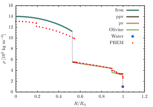
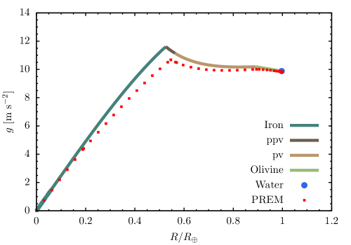
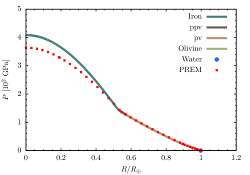
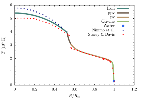
The structure Equations (A1)-(A5), along with Equation (A11) for each layer, are integrated from to with boundary conditions , , , , , and . The quantities and are the central pressure and temperature of the planet, whereas and are the pressure and temperature at the surface of the condensed part, i.e., at the bottom of the gaseous envelope, both provided by the envelope structure calculations. The set of equations is numerically solved by means of a suite of implicit/explicit algorithms. In the case of a stiff problem, an algorithm based on backward differentiation formulas (i.e., the Gear method, Gear, 1971) is employed. If the problem is non-stiff, the Adams-Moulton method (Hairer et al., 1993) is used instead. If implicit methods encounter difficulties, a variable high-order extrapolation algorithm of variable step-size, based on the Gragg-Bulirsch-Stoer method (Hairer et al., 1993), is used. The marching step () is self-adaptive and is constrained to be smaller than the smallest of , computed locally for . The integration is repeated, applying a search algorithm in order to adjust and , until and are within a few percent (% for thermal calculations) of the boundary conditions and .
| Planet | (Fe,Si,H2O)% | aaSimplified structure models. | aaSimplified structure models. | bbImproved structure models. | bbImproved structure models. | bbImproved structure models. | |
|---|---|---|---|---|---|---|---|
| b | |||||||
| c | |||||||
| d | |||||||
| e | |||||||
| f | |||||||
| g |
The core structure calculations used for the ex situ models, discussed in Section 2.2, are simplified in that they use only mass continuity, Equation (A1), and hydrostatic equilibrium, Equation (A2), to compute , imposing the conditions (). Moreover, they assume that the iron core is entirely made of -Fe and the H2O shell of ice VII-X. Here we intend to check how the improved structures (i.e., with thermodynamics and additional material phases) compare to those adopted to construct ex situ models.
Table A reports test results from the structures of planets and satellites of the solar system, both in the simplified and improved version. Comparisons are carried out for the radius and the moment of inertia factor (MoI). The simplified models reproduce quite accurately the radii of these bodies. In the tests, as expected, the thermal structure of the improved models provides only minor (and sometimes minute) adjustments to the radius. Nonetheless, the results indicate that the thermal models produce reasonable interior structures. Clearly, the adopted compositional partition into two/three layers represents the single major factor determining the radius and the MoI of these bodies. Of the simulated bodies, it should be noted that the iron mass fraction of the Moon is quite uncertain, yet both models provide a iron core radius of , in agreement with detection from seismic analysis (Weber et al., 2011). The MoI of Venus and Triton are undetermined, and the value of in Table A is assumed as representative of fully differentiated bodies (e.g., Chen et al., 2014). The largest discrepancies are obtained for the MoI of Callisto and Titan, which is likely due to the adopted compositions and complete differentiation assumption. Callisto, for example, may have an intermediate silicate/ice mixed layer atop the silicate core (Sohl et al., 2002). None of the models in Table A predicts the presence of the low-pressure -Fe phase, whereas -Fe is predicted in Mercury, Mars, and the satellites. Therefore, only the high-pressure and liquid phases of iron are expected in the condensed part of the Kepler 11 planets discussed above.
Appendix B An Earth’s Model
Figure 18 displays a more detailed comparison of the improved structure model of the Earth (solid line), compared to the Preliminary Reference Earth Model (PREM, Dziewonski & Anderson, 1981) and to the geotherm of Stacey & Davis (2008), represented as red squares and diamonds respectively (see the legend). The structure calculation in the figure also includes an “ocean” layer (see the top-left panel), % water by mass (Stacey & Davis, 2008). The agreement is generally good, with the largest differences confined to the metallic core.
Mantle semi-convection successfully reproduces the temperature gradient in the Earth’s outer layers (see also Turcotte & Schubert, 2014) and in the mantle in general. The temperature at the CMB is , in accord with current estimates (Alfè et al., 2007; Kamada et al., 2012). The discrepancies in pressure and density in the core are expected (see also Valencia et al., 2006; Wagner et al., 2011) since only pure iron is considered and the presence of lighter elements, such as H, O, Si, and S (e.g., Alfè et al., 2007; Vočadlo, 2015, pp. 117-147), is neglected333It is also estimated that the Earth’s core may contain up to about % Ni by mass (Vočadlo, 2015, pp. 117-147).. These impurities are believed to reduce the core density by roughly % relative to that of pure iron, at the same conditions of pressure and temperature (Alfè et al., 2007). The inner part of the metallic core is believed to be less polluted than is the outer (liquid) part. The calculated core radius is % smaller than predicted by the PREM, . The absence of iron alloyed with lighter elements also prevents the formation of an outer molten core. In fact, the melting temperature of Fe at the CMB pressure of is around (Anzellini et al., 2013), whereas the melting temperature at that pressure of, e.g., iron sulfide (FeS) is around (Anderson & Ahrens, 1996). A calculation conducted with the Vinet EoS for -Fe of Anderson et al. (2001) yields core pressures, temperature, and densities that differ by % from those in Figure 18.
Core temperatures are quite uncertain, with suggested maximum values ranging up to , and maybe above (Sola & Alfè, 2009; Anzellini et al., 2013). As a reference, the bottom-right panel also shows the core adiabat of Nimmo et al. (2004), anchored at the CMB temperature. Again, the general agreement indicates that the thermal model performs reasonably well.
Appendix C Thermal Structures of the Solid Interiors of Kepler 11 Planets
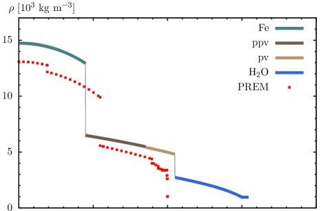
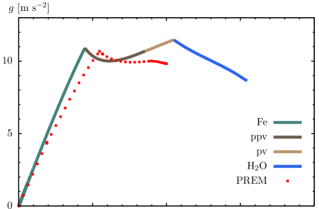
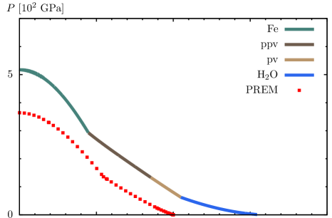
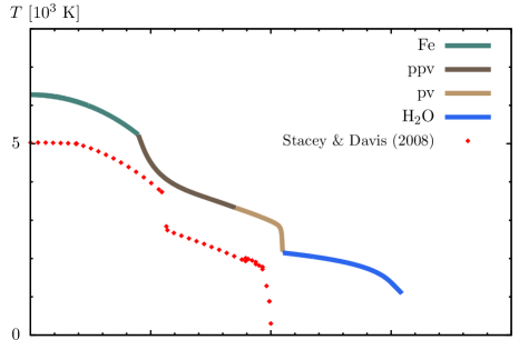
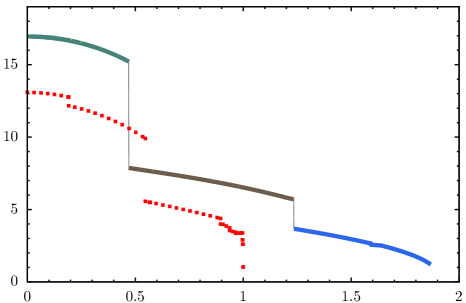
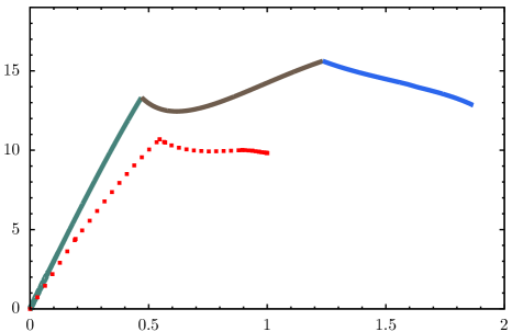
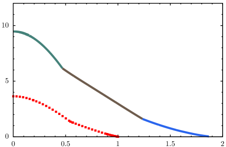
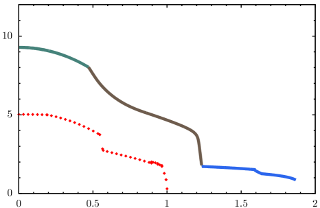
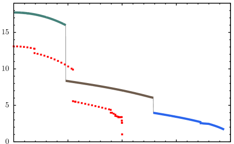
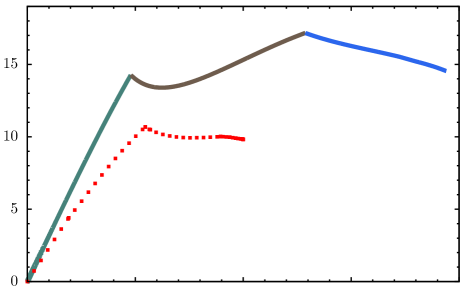
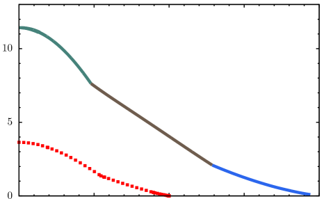
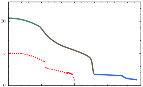
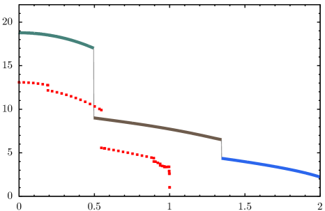
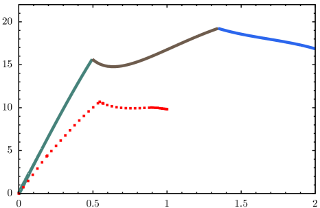
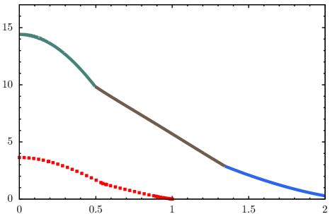

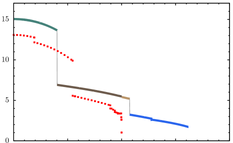
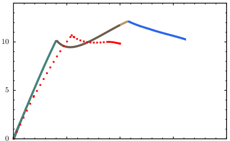
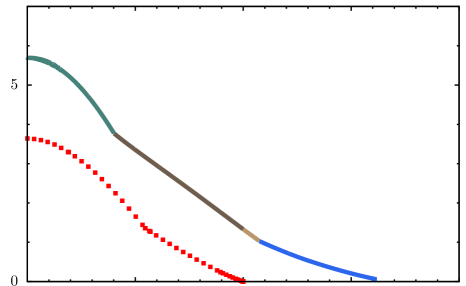
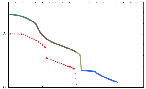
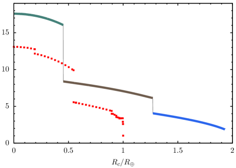
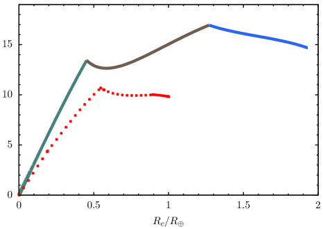
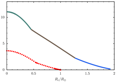
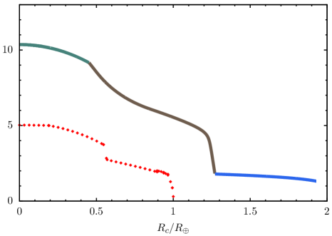
As mentioned above, at least % of Kepler 11 planets’ total mass consists of condensed material, hence the importance of the condensed structure of the planets in determining their radii. In this appendix, the radii and moment of inertia factors derived from isothermal models of the condensed interiors, applied in the main text, are compared to those derived from the improved structure models described in Appendix A. It should be pointed out that not all condensed layers of the simulated planets are in a solid phase, as liquid iron and liquid/superionic H2O may exist as well. Results from this comparison are listed in Tables 8.
In order to asses the impact of interior thermodynamics, the structure of the cores of the simulated planets was re-calculated applying core-envelope boundary pressures and temperatures ( and ) obtained from the ex situ calculations discussed in Section 4, at the age of (see Figure 19). The pressure ranges from to , whereas the temperature is between a little over and . Clearly, the values are unconstrained in the case of Kepler 11b, since no light-element envelope is present at . However, assuming the presence of a relatively thick steam atmosphere, the values and are applied. The differences between thermal and isothermal core radii are small, less than % in most cases and somewhat less than for Kepler 11c. The addition of thermal pressure, the second term on the right-hand side of Equation (A11), tends to reduce density and increase . However, there are additional effects to consider when comparing the two types of models. For example, H2O in isothermal cores is all in condensed form, whereas the liquid and superionic phases are, in fact, predominant in thermal models.
The case of Kepler 11b is more difficult to evaluate. The choice of and (stated above) leads to a % larger , compared to its isothermal counterpart. Upward and downward variations of a factor of two in boundary pressure produce a total change in core radius . If a thinner steam atmosphere could account for the observed radius, assuming a near-isothermal structure at the equilibrium temperature, , a boundary pressure would still provide a core radius only about % larger than that in Table 8 (and %, , larger than the isothermal radius). Significantly more inflated cores, and H2O shells in particular, would require much thinner atmospheres (e.g., for , see also Thomas & Madhusudhan, 2016), although it is not clear whether this possibility is relevant to Kepler 11b.
The results of Table 8 also indicate that the moment of inertia at is well approximated by isothermal models. The last column lists the energy flux at the core surface, , normalized to the average surface flux of the Earth, (Turcotte & Schubert, 2014). As explained above, these values are based on radiogenic heating rates in the planets’ silicate mantles estimated for the Earth (at its present age). The total energy output of the cores, , is negligible compared to the luminosities reported in Table 4. Experiments conducted on Kepler 11b and e with heating rates reduced by a factor of two () resulted in very similar interiors ( and the MoI factor differing by %, and at differing by %, and at differing by –%). The surface heat flux, , was instead reduced by a factor of .
Figure 19 shows some structural properties of Kepler 11 condensed interiors at . The density, gravitational acceleration, pressure, and temperature are plotted along with the PREM and the reference geotherm of Stacey & Davis (2008), as indicated in the legends of the top panels. As mentioned above, the core temperatures of the Earth may actually be higher. The temperature at the inner core boundary of the Earth (, , Dziewonski & Anderson, 1981) was estimated to be (Anzellini et al., 2013), based on an experimental determination of the melting curve of Fe (though uncertainties persist, e.g., Alfè, 2009; Aquilanti et al., 2015; Vočadlo, 2015, pp. 117-147).
The iron nucleus of all simulated planets is in the solid phase. The interior models of Figure 12, however, have totally or partially molten nuclei at early isolation times, –. Moreover, if iron in the nucleus was alloyed with lighter elements (such as sulfur or oxygen), a significant volume fraction would likely be in the liquid phase, due to lower melting temperatures (e.g., Anderson & Ahrens, 1996; Sotin et al., 2007; Morard et al., 2014). It is also likely that the presence of iron alloys would cause a (partially) molten nucleus in (at least some of) the planets at . For example, the CMB pressures of Kepler 11b and f are and , respectively. The melting temperature of FeS at these pressures is between and (Anderson & Ahrens, 1996), lower than the calculated CMB temperatures of those planets. It should be stressed, though, that sulfur and oxygen are among the impurities that produce the largest depression of the melting curve compared to that of pure iron (Terasaki & Fischer, 2016).
The silicate mantles contain only the high-pressure phases perovskite (pv) and post-perovskite (ppv). In fact, the transition between olivine and perovskite happens at pressures around (for , Fei et al., 2004), whereas pressures at the bottom of the H2O shell are in excess of . For the largest planets Kepler 11c, d, e, and g, the pressure at the base of the H2O shell is , so that ppv is the only phase present in their silicate mantles. Post-post-perovskite phases are predicted for (Wagner et al., 2012), a value reached only at the bottom of the mantle of Kepler 11e (although the stability field of post-ppv phases is also determined by temperature, Stamenković et al., 2011). The H2O shell is mostly in fluid/superionic phase, except for the presence of ice VII layers in the outer parts of Kepler 11c, d and f.
The interior structures in Figure 19 can be qualitatively compared to those presented by Wagner et al. (2012, , see their Figure 1), since the structural and thermal model applied here share a number of similarities to theirs. However, a detailed comparison is not possible. They considered super-Earths with an Earth-like composition and Earth-like conditions at the surface. Masses are also different from those of Kepler 11 planets. Because of the assumed composition, their planets have radii smaller than those obtained here, for similar core masses. Consequently, their central pressures are higher, . Mantle temperatures are different, which could depend on the boundary conditions at the surface, on the presence of the H2O shell, and on the behavior of semi-convection in the outer layers of the silicate mantles. In fact, these layers behave as a stagnant lid, in which heat is mainly transported via conduction. The temperature gain across the lid typically accounts for –% of the temperature gain across the entire mantle. The details of the temperature gradient in the lid depend on the thermal conductivity , which is still poorly constrained in the high-pressure and temperature ranges of pv and ppv phases (e.g., see the discussion in van den Berg et al., 2010; Stamenković et al., 2011; Hunt et al., 2012; Wagner et al., 2012). Heat transport becomes more efficient as convection grows more and more vigorous with depth, underneath the stagnant lid. However, details of mantle convection depend on the assumed viscosity parametrization, which is different between the two studies.
The temperatures deep down in the mantles may exceed the melting temperatures of silicates so that, instead of Equation (A4), the adiabatic temperature gradient in Equation (A5) would apply to those layers. The – curves of the mantles in Figure 19 were compared to the high-pressure melting curve of silica (SiO2) recently determined by Millot et al. (2015) via shock-compression experiments. It was found that in none of the planets’ mantles the temperature rises above the melting point. The situation may be different at earlier epochs, though, before the planets cool down. In the case of Kepler 11e, it was found that over most of the evolution in isolation, , mantle temperatures lie below the melting curve. At earlier times, however, the mantle is entirely molten (according to the experiments of Millot et al., 2015) and, hence, it may be approximated as adiabatic. For the less massive planets, Kepler 11c and f, mantle temperatures drop below the melting curve at earlier times, –.
Figure 12 shows that the condensed cores of Kepler 11 planets formed ex situ (i.e., with significant H2O content) can undergo substantial contraction during the early stages of evolution in isolation. By , however, the cores are within a few percent of their current radii in Table 8. As mentioned in Section 4.3, almost all of the contraction takes place in the outer H2O shells, and only –% of the total difference shown in Figure 12 is caused by the contraction of nucleus and mantle. In fact, assuming that the condensed core of Kepler 11g (which undergoes a contraction corresponding to ) was % Fe and % Si by mass, the difference in radii between and would be only ! The average gravitational energy per unit time released by the contraction of the cores in Figure 12, during the first of evolution, is , becoming much smaller during the following .
References
- Abe (1995) Abe, Y. 1995, in The Earth’s Central Part: Its Structure and Dynamic, ed. T. Yukutake (Tokyo: Terra Scientific Publishing Company), 215–230
- Abe (1997) Abe, Y. 1997, Physics of the Earth and Planetary Interiors, 100, 27
- Abramson & Brown (2004) Abramson, H. E., & Brown, M. J. 2004, Geochimica et Cosmochimica Acta, 68, 1827
- Alexander & Armitage (2007) Alexander, R. D., & Armitage, P. J. 2007, MNRAS, 375, 500
- Alfè (2009) Alfè, D. 2009, Phys. Rev. B, 79, 060101
- Alfè et al. (2007) Alfè, D., J., G. M., & Price, G. D. 2007, Contemporary Physics, 48, 63
- Al’tshuler et al. (1987) Al’tshuler, L., Brusnikin, S., & Kuz’menkov, E. 1987, Journal of Applied Mechanics and Technical Physics, 28, 129
- Anderson (1989) Anderson, D. L. 1989, Theory of the Earth (Oxford, UK: Blackwell Scientific Publications)
- Anderson (1995) Anderson, O. L. 1995, Equations of State of Solids for Geophysics and Ceramic Science (New York: Oxford University Press)
- Anderson et al. (2001) Anderson, O. L., Dubrovinsky, L., Saxena, S. K., & LeBihan, T. 2001, Geophysical Research Letters, 28, 399
- Anderson & Ahrens (1996) Anderson, W. W., & Ahrens, T. J. 1996, Journal of Geophysical Research: Solid Earth, 101, 5627
- Anzellini et al. (2013) Anzellini, S., Dewaele, A., Mezouar, M., Loubeyre, P., & Morard, G. 2013, Science, 340, 464
- Aquilanti et al. (2015) Aquilanti, G., Trapananti, A., Karandikar, A., Kantor, I., Marini, C., Mathon, O., Pascarelli, S., & Boehler, R. 2015, Proceedings of the National Academy of Sciences of the United States of America, 112, 12042
- Artymowicz (1993) Artymowicz, P. 1993, ApJ, 419, 166
- Asplund et al. (2009) Asplund, M., Grevesse, N., Sauval, A. J., & Scott, P. 2009, ARA&A, 47, 481
- Barr & Showman (2009) Barr, A. C., & Showman, A. P. 2009, in Europa, ed. R. T. Pappalardo, W. B. McKinnon, & K. K. Khurana (Tucson, AZ: University of Arizona Press), 405
- Baruteau et al. (2014) Baruteau, C., Crida, A., Paardekooper, S.-J., Masset, F., Guilet, J., Bitsch, B., Nelson, R., Kley, W., & Papaloizou, J. 2014, in Protostars and Planets VI, ed. H. Beuther, R. S. Klessen, C. P. Dullemond, & T. Henning (Tucson, AZ: University of Arizona Press), 667–689
- Baruteau & Papaloizou (2013) Baruteau, C., & Papaloizou, J. C. B. 2013, ApJ, 778, 7
- Batygin (2015) Batygin, K. 2015, MNRAS, 451, 2589
- Batygin & Morbidelli (2013) Batygin, K., & Morbidelli, A. 2013, AJ, 145, 1
- Bodenheimer et al. (2013) Bodenheimer, P., D’Angelo, G., Lissauer, J. J., Fortney, J. J., & Saumon, D. 2013, Astrophys. J., 770, 120
- Bodenheimer et al. (2000) Bodenheimer, P., Hubickyj, O., & Lissauer, J. J. 2000, Icarus, 143, 2
- Bodenheimer et al. (2006) Bodenheimer, P., Laughlin, G., Rózyczka, M., & Yorke, H. 2006, Numerical Methods in Astrophysics: An Introduction (Boca Raton, FL: CRC Press, Taylor and Francis Group)
- Bodenheimer & Lissauer (2014) Bodenheimer, P., & Lissauer, J. J. 2014, ApJ, 791, 103
- Bodenheimer & Pollack (1986) Bodenheimer, P., & Pollack, J. B. 1986, Icarus, 67, 391
- Borsato et al. (2014) Borsato, L., Marzari, F., Nascimbeni, V., Piotto, G., Granata, V., Bedin, L. R., & Malavolta, L. 2014, A&A, 571, A38
- Boshkayev et al. (2016) Boshkayev, K. A., Rueda, J. A., Zhami, B. A., Kalymova, Z. A., & Balgymbekov, G. S. 2016, International Journal of Modern Physics: Conference Series, 41, 1660129
- Chatterjee & Ford (2015) Chatterjee, S., & Ford, E. B. 2015, ApJ, 803, 33
- Chen et al. (2014) Chen, E. M. A., Nimmo, F., & Glatzmaier, G. A. 2014, Icarus, 229, 11
- Chiang & Laughlin (2013) Chiang, E., & Laughlin, G. 2013, MNRAS, 431, 3444
- Chiang & Goldreich (1999) Chiang, E. I., & Goldreich, P. 1999, ApJ, 519, 279
- Choukroun & Grasset (2007) Choukroun, M., & Grasset, O. 2007, The Journal of Chemical Physics, 127, 124506
- Cowan & Ashkin (1957) Cowan, R. D., & Ashkin, J. 1957, Phys. Rev., 105, 144
- Cox (1968) Cox, J. P. 1968, Principles of Stellar Structure - Vol.1: Physical principles; Vol.2: Applications to Stars (New York: Gordon and Breach)
- D’Angelo & Bodenheimer (2013) D’Angelo, G., & Bodenheimer, P. 2013, ApJ, 778, 77
- D’Angelo & Lubow (2008) D’Angelo, G., & Lubow, S. H. 2008, ApJ, 685, 560
- D’Angelo & Lubow (2010) —. 2010, ApJ, 724, 730
- D’Angelo et al. (2006) D’Angelo, G., Lubow, S. H., & Bate, M. R. 2006, ApJ, 652, 1698
- D’Angelo & Marzari (2012) D’Angelo, G., & Marzari, F. 2012, ApJ, 757, 50
- D’Angelo & Podolak (2015) D’Angelo, G., & Podolak, M. 2015, ApJ, 806, 203
- D’Angelo et al. (2014) D’Angelo, G., Weidenschilling, S. J., Lissauer, J. J., & Bodenheimer, P. 2014, Icarus, 241, 298
- Davis (2005) Davis, S. S. 2005, ApJ, 627, L153
- de Carvalho et al. (2014) de Carvalho, S. M., Rotondo, M., Rueda, J. A., & Ruffini, R. 2014, Phys. Rev. C, 89, 015801
- de Koker et al. (2012) de Koker, N., Steinle-Neumann, G., & Vlček, V. 2012, Proceedings of the National Academy of Sciences, 109, 4070
- Deck & Batygin (2015) Deck, K. M., & Batygin, K. 2015, ApJ, 810, 119
- Delisle et al. (2012) Delisle, J.-B., Laskar, J., Correia, A. C. M., & Boué, G. 2012, A&A, 546, A71
- Dewaele et al. (2006) Dewaele, A., Loubeyre, P., Occelli, F., Mezouar, M., Dorogokupets, P. I., & Torrent, M. 2006, Phys. Rev. Lett., 97, 215504
- Dodson-Robinson et al. (2009) Dodson-Robinson, S. E., Willacy, K., Bodenheimer, P., Turner, N. J., & Beichman, C. A. 2009, Icarus, 200, 672
- Durham & Stern (2001) Durham, W. B., & Stern, L. A. 2001, Annual Review of Earth and Planetary Sciences, 29, 295
- Durisen et al. (2007) Durisen, R. H., Boss, A. P., Mayer, L., Nelson, A. F., Quinn, T., & Rice, W. K. M. 2007, in Protostars and Planets V, ed. B. Reipurth, D. Jewitt, & K. Keil (Tucson, AZ: University of Arizona Press), 607–622
- Dziewonski & Anderson (1981) Dziewonski, A. M., & Anderson, D. L. 1981, Physics of the Earth and Planetary Interiors, 25, 297
- Erkaev et al. (2007) Erkaev, N. V., Kulikov, Y. N., Lammer, H., Selsis, F., Langmayr, D., Jaritz, G. F., & Biernat, H. K. 2007, A&A, 472, 329
- Fabrycky et al. (2014) Fabrycky, D. C., Lissauer, J. J., Ragozzine, D., Rowe, J. F., Steffen, J. H., Agol, E., Barclay, T., Batalha, N., Borucki, W., Ciardi, D. R., Ford, E. B., Gautier, T. N., Geary, J. C., Holman, M. J., Jenkins, J. M., Li, J., Morehead, R. C., Morris, R. L., Shporer, A., Smith, J. C., Still, M., & Van Cleve, J. 2014, ApJ, 790, 146
- Fei et al. (1993) Fei, Y., Mao, H., & Hemley, R. J. 1993, The Journal of Chemical Physics, 99, 5369
- Fei et al. (2004) Fei, Y., Van Orman, J., Li, J., van Westrenen, W., Sanloup, C., Minarik, W., Hirose, K., Komabayashi, T., Walter, M., & Funakoshi, K. 2004, Journal of Geophysical Research: Solid Earth, 109, B02305
- Ferguson et al. (2005) Ferguson, J. W., Alexander, D. R., Allard, F., Barman, T., Bodnarik, J. G., Hauschildt, P. H., Heffner-Wong, A., & Tamanai, A. 2005, ApJ, 623, 585
- Figueira et al. (2012) Figueira, P., Marmier, M., Boué, G., Lovis, C., Santos, N. C., Montalto, M., Udry, S., Pepe, F., & Mayor, M. 2012, A&A, 541, A139
- Fortes et al. (2005) Fortes, A. D., Wood, I. G., Alfredsson, M., Vočadlo, L., & Knight, K. S. 2005, Journal of Applied Crystallography, 38, 612
- Frank et al. (2004) Frank, M. R., Fei, Y., & Hu, J. 2004, Geochimica et Cosmochimica Acta, 68, 2781
- Freedman et al. (2008) Freedman, R. S., Marley, M. S., & Lodders, K. 2008, ApJS, 174, 504
- French et al. (2009) French, M., Mattsson, T. R., Nettelmann, N., & Redmer, R. 2009, Phys. Rev. B, 79, 054107
- Fu et al. (2010) Fu, R., O’Connell, R. J., & Sasselov, D. D. 2010, ApJ, 708, 1326
- Gear (1971) Gear, G. W. 1971, Numerical Initial Value Problems in Ordinary Differential Equations (Englewood Cliffs, NJ: Prentice-Hall)
- Ginzburg et al. (2016) Ginzburg, S., Schlichting, H. E., & Sari, R. 2016, ApJ, 825, 29
- Goldreich & Schlichting (2014) Goldreich, P., & Schlichting, H. E. 2014, AJ, 147, 32
- Gorti et al. (2009) Gorti, U., Dullemond, C. P., & Hollenbach, D. 2009, ApJ, 705, 1237
- Gorti & Hollenbach (2009) Gorti, U., & Hollenbach, D. 2009, ApJ, 690, 1539
- Greenzweig & Lissauer (1990) Greenzweig, Y., & Lissauer, J. J. 1990, Icarus, 87, 40
- Greenzweig & Lissauer (1992) —. 1992, Icarus, 100, 440
- Guillot (2010) Guillot, T. 2010, A&A, 520, A27
- Hadden & Lithwick (2014) Hadden, S., & Lithwick, Y. 2014, ApJ, 787, 80
- Hairer et al. (1993) Hairer, E., Nørsett, S. P., & Wanner, G. 1993, Solving Ordinary Differential Equations I: Nonstiff Problems (Berlin: Springer)
- Hands et al. (2014) Hands, T. O., Alexander, R. D., & Dehnen, W. 2014, MNRAS, 445, 749
- Hansen & Murray (2012) Hansen, B. M. S., & Murray, N. 2012, ApJ, 751, 158
- Hansen & Murray (2013) —. 2013, ApJ, 775, 53
- Hayashi (1981) Hayashi, C. 1981, Progress of Theoretical Physics Supplement, 70, 35
- Hofmeister (1999) Hofmeister, A. M. 1999, Science, 283, 1699
- Hollenbach et al. (1994) Hollenbach, D., Johnstone, D., Lizano, S., & Shu, F. 1994, ApJ, 428, 654
- Howard et al. (2010) Howard, A. W., Marcy, G. W., Johnson, J. A., Fischer, D. A., Wright, J. T., Isaacson, H., Valenti, J. A., Anderson, J., Lin, D. N. C., & Ida, S. 2010, Science, 330, 653
- Hubeny (1990) Hubeny, I. 1990, ApJ, 351, 632
- Hubickyj et al. (2005) Hubickyj, O., Bodenheimer, P., & Lissauer, J. J. 2005, Icarus, 179, 415
- Hunt et al. (2012) Hunt, S. A., Davies, D. R., Walker, A. M., McCormack, R. J., Wills, A. S., Dobson, D. P., & Li, L. 2012, Earth and Planetary Science Letters, 319–320, 96
- Ichikawa et al. (2014) Ichikawa, H., Tsuchiya, T., & Tange, Y. 2014, Journal of Geophysical Research: Solid Earth, 119, 240
- Ida & Lin (2004) Ida, S., & Lin, D. N. C. 2004, ApJ, 604, 388
- Iglesias & Rogers (1996) Iglesias, C. A., & Rogers, F. J. 1996, ApJ, 464, 943
- Ikoma & Hori (2012) Ikoma, M., & Hori, Y. 2012, ApJ, 753, 66
- Jackson & Rigden (1996) Jackson, I., & Rigden, S. M. 1996, Physics of the Earth and Planetary Interiors, 96, 85
- Kamada et al. (2012) Kamada, S., Ohtani, E., Terasaki, H., Sakai, T. a. M., Ohishi, Y., & Hirao, N. 2012, Earth and Planetary Science Letters, 359, 26
- Katsura et al. (2009a) Katsura, T., Shatskiy, A., Manthilake, G., Zhai, S., Fukui, H., Yamazaki, D., Matsuzaki, T., Yoneda, A., Ito, E., Kuwata, A., Ueda, A., Nozawa, A., & Funakoshi, K. 2009a, Physics of the Earth and Planetary Interiors, 174, 86
- Katsura et al. (2009b) Katsura, T., Yokoshi, S., Kawabe, K., Shatskiy, A., Manthilake, G., Zhai, S., Fukui, H., Hegoda, C., Yoshino, T., Yamazaki, D., Matsuzaki, T., Yoneda, A., Ito, E., Sugita, M., Tomioka, N., Hagiya, K., Nozawa, A., & Funakoshi, K. 2009b, Geophysical Research Letters, 36, L01305
- Kerley (1993) Kerley, I. G. 1993, Multiphase Equation of State for Iron, Tech. Rep. SAND93-0027 (Albuquerque, NM, and Livermore, CA: Sandia National Laboratories)
- Kippenhahn et al. (2013) Kippenhahn, R., Weigert, A., & Weiss, A. 2013, Stellar Structure and Evolution (Berlin: Springer)
- Kley & Nelson (2012) Kley, W., & Nelson, R. P. 2012, ARA&A, 50, 211
- Komabayashi & Fei (2010) Komabayashi, T., & Fei, Y. 2010, Journal of Geophysical Research: Solid Earth, 115, 1–12
- Lee & Chiang (2015) Lee, E. J., & Chiang, E. 2015, ApJ, 811, 41
- Liffman (2003) Liffman, K. 2003, Publications of the Astronomical Society of Australia, 20, 337
- Lin & Papaloizou (1986) Lin, D. N. C., & Papaloizou, J. 1986, ApJ, 309, 846
- Lin et al. (2005) Lin, J.-F., Gregoryanz, E., Struzhkin, V. V., Somayazulu, M., Mao, H.-k., & Hemley, R. J. 2005, Geophysical Research Letters, 32, L11306
- Lin et al. (2004) Lin, J.-F., Militzer, B., Struzhkin, V. V., Gregoryanz, E., Hemley, R. J., & Mao, H.-k. 2004, The Journal of Chemical Physics, 121, 8423
- Lissauer et al. (2011a) Lissauer, J. J., Fabrycky, D. C., Ford, E. B., Borucki, W. J., Fressin, F., Marcy, G. W., Orosz, J. A., Rowe, J. F., Torres, G., Welsh, W. F., Batalha, N. M., Bryson, S. T., Buchhave, L. A., Caldwell, D. A., Carter, J. A., Charbonneau, D., Christiansen, J. L., Cochran, W. D., Desert, J.-M., Dunham, E. W., Fanelli, M. N., Fortney, J. J., Gautier, III, T. N., Geary, J. C., Gilliland, R. L., Haas, M. R., Hall, J. R., Holman, M. J., Koch, D. G., Latham, D. W., Lopez, E., McCauliff, S., Miller, N., Morehead, R. C., Quintana, E. V., Ragozzine, D., Sasselov, D., Short, D. R., & Steffen, J. H. 2011a, Nature, 470, 53
- Lissauer et al. (2009) Lissauer, J. J., Hubickyj, O., D’Angelo, G., & Bodenheimer, P. 2009, Icarus, 199, 338
- Lissauer et al. (2013) Lissauer, J. J., Jontof-Hutter, D., Rowe, J. F., Fabrycky, D. C., Lopez, E. D., Agol, E., Marcy, G. W., Deck, K. M., Fischer, D. A., Fortney, J. J., Howell, S. B., Isaacson, H., Jenkins, J. M., Kolbl, R., Sasselov, D., Short, D. R., & Welsh, W. F. 2013, ApJ, 770, 131
- Lissauer et al. (2011b) Lissauer, J. J., Ragozzine, D., Fabrycky, D. C., Steffen, J. H., Ford, E. B., Jenkins, J. M., Shporer, A., Holman, M. J., Rowe, J. F., Quintana, E. V., Batalha, N. M., Borucki, W. J., Bryson, S. T., Caldwell, D. A., Carter, J. A., Ciardi, D., Dunham, E. W., Fortney, J. J., Gautier, III, T. N., Howell, S. B., Koch, D. G., Latham, D. W., Marcy, G. W., Morehead, R. C., & Sasselov, D. 2011b, ApJS, 197, 8
- Lithwick & Wu (2012) Lithwick, Y., & Wu, Y. 2012, ApJ, 756, L11
- Lodders (2010) Lodders, K. 2010, in Principles and Perspectives in Cosmochemistry, ed. A. Goswami & B. E. Reddy (Berlin: Springer), 379
- Lopez et al. (2012) Lopez, E. D., Fortney, J. J., & Miller, N. 2012, ApJ, 761, 59
- Loubeyre et al. (1999) Loubeyre, P., LeToullec, R., Wolanin, E., Hanfland, M., & Hausermann, D. 1999, Nature, 397, 503
- Lubow & D’Angelo (2006) Lubow, S. H., & D’Angelo, G. 2006, ApJ, 641, 526
- Lubow & Ida (2011) Lubow, S. H., & Ida, S. 2011, in Exoplanets, ed. S. Seager (Tucson, AZ: University of Arizona Press), 347–371
- Lynden-Bell & Pringle (1974) Lynden-Bell, D., & Pringle, J. E. 1974, MNRAS, 168, 603
- Masset & Casoli (2010) Masset, F. S., & Casoli, J. 2010, ApJ, 723, 1393
- McNeil & Nelson (2010) McNeil, D. S., & Nelson, R. P. 2010, MNRAS, 401, 1691
- Menou & Goodman (2004) Menou, K., & Goodman, J. 2004, ApJ, 606, 520
- Meyer-Vernet & Sicardy (1987) Meyer-Vernet, N., & Sicardy, B. 1987, Icarus, 69, 157
- Migaszewski et al. (2012) Migaszewski, C., Słonina, M., & Goździewski, K. 2012, MNRAS, 427, 770
- Mihalas & Weibel Mihalas (1999) Mihalas, D., & Weibel Mihalas, B. 1999, Foundations of Radiation Hydrodynamics (New York: Dover)
- Millot et al. (2015) Millot, M., Dubrovinskaia, N., Černok, A., Blaha, S., Dubrovinsky, L., Braun, D. G., Celliers, P. M., Collins, G. W., Eggert, J. H., & Jeanloz, R. 2015, Science, 347, 418
- Minton & Levison (2014) Minton, D. A., & Levison, H. F. 2014, Icarus, 232, 118
- Morard et al. (2014) Morard, G., Andrault, D., Antonangeli, D., & Bouchet, J. 2014, Comptes Rendus Geoscience, 346, 130
- Mordasini et al. (2012) Mordasini, C., Alibert, Y., Georgy, C., Dittkrist, K.-M., Klahr, H., & Henning, T. 2012, A&A, 547, A112
- Movshovitz et al. (2010) Movshovitz, N., Bodenheimer, P., Podolak, M., & Lissauer, J. J. 2010, Icarus, 209, 616
- Mullally et al. (2015) Mullally, F., Coughlin, J. L., Thompson, S. E., Rowe, J., Burke, C., Latham, D. W., Batalha, N. M., Bryson, S. T., Christiansen, J., Henze, C. E., Ofir, A., Quarles, B., Shporer, A., Van Eylen, V., Van Laerhoven, C., Shah, Y., Wolfgang, A., Chaplin, W. J., Xie, J.-W., Akeson, R., Argabright, V., Bachtell, E., Barclay, T., Borucki, W. J., Caldwell, D. A., Campbell, J. R., Catanzarite, J. H., Cochran, W. D., Duren, R. M., Fleming, S. W., Fraquelli, D., Girouard, F. R., Haas, M. R., Hełminiak, K. G., Howell, S. B., Huber, D., Larson, K., Gautier, III, T. N., Jenkins, J. M., Li, J., Lissauer, J. J., McArthur, S., Miller, C., Morris, R. L., Patil-Sabale, A., Plavchan, P., Putnam, D., Quintana, E. V., Ramirez, S., Silva Aguirre, V., Seader, S., Smith, J. C., Steffen, J. H., Stewart, C., Stober, J., Still, M., Tenenbaum, P., Troeltzsch, J., Twicken, J. D., & Zamudio, K. A. 2015, ApJS, 217, 31
- Murray-Clay et al. (2009) Murray-Clay, R. A., Chiang, E. I., & Murray, N. 2009, ApJ, 693, 23
- Nimmo et al. (2004) Nimmo, F., Price, G. D., Brodholt, J., & Gubbins, D. 2004, Geophysical Journal International, 156, 363
- Ogihara et al. (2015) Ogihara, M., Morbidelli, A., & Guillot, T. 2015, A&A, 578, A36
- Owen & Wu (2016) Owen, J. E., & Wu, Y. 2016, ApJ, 817, 107
- Paardekooper et al. (2011) Paardekooper, S.-J., Baruteau, C., & Kley, W. 2011, MNRAS, 410, 293
- Phillips & Malin (1983) Phillips, R. J., & Malin, M. C. 1983, in Venus, ed. D. M. Hunten, L. Colin, T. M. Donahue, an V. I. Moroz (Tucson, AZ: University of Arizona Press), 159–214
- Pollack et al. (1996) Pollack, J. B., Hubickyj, O., Bodenheimer, P., Lissauer, J. J., Podolak, M., & Greenzweig, Y. 1996, Icarus, 124, 62
- Pringle (1981) Pringle, J. E. 1981, ARA&A, 19, 137
- Redmer et al. (2011) Redmer, R., Mattsson, T. R., Nettelmann, N., & French, M. 2011, Icarus, 211, 798
- Rein (2012) Rein, H. 2012, MNRAS, 427, L21
- Reynard & Price (1990) Reynard, B., & Price, G. D. 1990, Geophysical Research Letters, 17, 689
- Ribas et al. (2005) Ribas, I., Guinan, E. F., Güdel, M., & Audard, M. 2005, ApJ, 622, 680
- Righter et al. (2006) Righter, K., Drake, M. J., & Scott, E. R. D. 2006, in Meteorites and the Early Solar System II, ed. D. S. Lauretta, and H. Y. McSween (Tucson, AZ: University of Arizona Press), 803–828
- Rogers et al. (2011) Rogers, L. A., Bodenheimer, P., Lissauer, J. J., & Seager, S. 2011, ApJ, 738, 59
- Safronov (1969) Safronov, V. S. 1969, Evolution of the Protoplanetary Cloud and Formation of the Earth and Planets (Moscow: Nauka Press)
- Salpeter & Zapolsky (1967) Salpeter, E. E., & Zapolsky, H. S. 1967, Physical Review, 158, 876
- Sasaki & Nakazawa (1986) Sasaki, S., & Nakazawa, K. 1986, J. Geophys. Res., 91, 9231
- Saumon et al. (1995) Saumon, D., Chabrier, G., & van Horn, H. M. 1995, ApJS, 99, 713
- Schlichting (2014) Schlichting, H. E. 2014, ApJ, 795, L15
- Seager et al. (2007) Seager, S., Kuchner, M., Hier-Majumder, C. A., & Militzer, B. 2007, ApJ, 669, 1279
- Seagle et al. (2013) Seagle, C. T., Cottrell, E., Fei, Y., Hummer, D. R., & Prakapenka, V. B. 2013, Geophysical Research Letters, 40, 5377
- Shakura & Sunyaev (1973) Shakura, N. I., & Sunyaev, R. A. 1973, A&A, 24, 337
- Siess et al. (2000) Siess, L., Dufour, E., & Forestini, M. 2000, A&A, 358, 593
- Sohl & Schubert (2007) Sohl, F., & Schubert, G. 2007, in Treatise on Geophysics, ed. G. Schubert (Amsterdam: Elsevier), 27–68
- Sohl et al. (2014a) Sohl, F., Solomonidou, A., Wagner, F. W., Coustenis, A., Hussmann, H., & Schulze-Makuch, D. 2014a, Journal of Geophysical Research: Planets, 119, 1013
- Sohl et al. (2002) Sohl, F., Spohn, T., Breuer, D., & Nagel, K. 2002, Icarus, 157, 104
- Sohl et al. (2014b) Sohl, F., Wagner, F. W., & Rauer, H. 2014b, in IAU Symp. 293, Formation, Detection, and Characterization of Extrasolar Habitable Planets, ed. N. Haghighipour (Cambridge: Cambridge University Press), 350
- Sola & Alfè (2009) Sola, E., & Alfè, D. 2009, Phys. Rev. Lett., 103, 078501
- Sotin et al. (2007) Sotin, C., Grasset, O., & Mocquet, A. 2007, Icarus, 191, 337
- Sotin & Tobie (2004) Sotin, C., & Tobie, G. 2004, Comptes Rendus Physique, 5, 769
- Soubiran & Militzer (2015) Soubiran, F., & Militzer, B. 2015, ApJ, 806, 228
- Spada et al. (2013) Spada, F., Demarque, P., Kim, Y.-C., & Sills, A. 2013, ApJ, 776, 87
- Stacey & Davis (2008) Stacey, F. D., & Davis, P. M. 2008, Physics of the Earth (Cambridge, UK: Cambridge University Press)
- Stamenković et al. (2011) Stamenković, V., Breuer, D., & Spohn, T. 2011, Icarus, 216, 572
- Stevenson (1982) Stevenson, D. J. 1982, Planet. Space Sci., 30, 755
- Stewart & Ahrens (2005) Stewart, S. T., & Ahrens, T. J. 2005, Journal of Geophysical Research: Planets, 110, E03005
- Stixrude & Bukowinski (1990) Stixrude, L., & Bukowinski, M. S. T. 1990, Journal of Geophysical Research: Solid Earth, 95, 19311
- Sun et al. (2015) Sun, J., Clark, B. K., Torquato, S., & Car, R. 2015, Nature Communications, 6, 753
- Tachinami et al. (2011) Tachinami, C., Senshu, H., & Ida, S. 2011, ApJ, 726, 70
- Tan et al. (2015) Tan, J. C., Chatterjee, S., Hu, X., Zhu, Z., & Mohanty, S. 2015, arXiv:1510.06703
- Tanaka (1998) Tanaka, H. 1998, The Journal of Chemical Physics, 108, 4887
- Tanaka et al. (2002) Tanaka, H., Takeuchi, T., & Ward, W. R. 2002, ApJ, 565, 1257
- Tanaka & Ward (2004) Tanaka, H., & Ward, W. R. 2004, ApJ, 602, 388
- Tateno et al. (2009) Tateno, S., Hirose, K., Sata, N., & Ohishi, Y. 2009, Earth and Planetary Science Letters, 277, 130
- Terasaki & Fischer (2016) Terasaki, H., & Fischer, R. A. 2016, Deep Earth: Physics and Chemistry of the Lower Mantle and Core (Hoboken, NJ: Wiley)
- Thomas & Madhusudhan (2016) Thomas, S. W., & Madhusudhan, N. 2016, MNRAS, 458, 1330
- Tobie et al. (2005) Tobie, G., Grasset, O., Lunine, J. I., Mocquet, A., & Sotin, C. 2005, Icarus, 175, 496
- Turcotte & Schubert (2014) Turcotte, D. L., & Schubert, G. 2014, Geodynamics (Cambridge, UK: Cambridge University Press)
- Valencia et al. (2006) Valencia, D., O’Connell, R. J., & Sasselov, D. 2006, Icarus, 181, 545
- van den Berg et al. (2010) van den Berg, A. P., D.A. Yuen, D. A., G.L. Beebe, G. L., & Christiansen, M. D. 2010, Physics of the Earth and Planetary Interiors, 178, 136
- Vočadlo (2015) Vočadlo, L. 2015, in Treatise on Geophysics, ed. G. Schubert (Oxford, UK: Elsevier), 117–147
- Wagner et al. (2011) Wagner, F. W., Sohl, F., Hussmann, H., Grott, M., & Rauer, H. 2011, Icarus, 214, 366
- Wagner et al. (2012) Wagner, F. W., Tosi, N., Sohl, F., Rauer, H., & Spohn, T. 2012, A&A, 541, A103
- Wagner & Pruß (2002) Wagner, W., & Pruß, A. 2002, Journal of Physical and Chemical Reference Data, 31, 387
- Ward (1997) Ward, W. R. 1997, Icarus, 126, 261
- Watson et al. (1981) Watson, A. J., Donahue, T. M., & Walker, J. C. G. 1981, Icarus, 48, 150
- Weber et al. (2011) Weber, R. C., Lin, P.-Y., Garnero, E. J., Williams, Q., & Lognonné, P. 2011, Science, 331, 309
- Weidenschilling (1977) Weidenschilling, S. J. 1977, Astrophysics and Space Science, 51, 153
- Williams & Cieza (2011) Williams, J. P., & Cieza, L. A. 2011, ARA&A, 49, 67
- Wilson et al. (2013) Wilson, H. F., Wong, M. L., & Militzer, B. 2013, Phys. Rev. Lett., 110, 151102
- Winn & Fabrycky (2015) Winn, J. N., & Fabrycky, D. C. 2015, ARA&A, 53, 409
- Zapolsky & Salpeter (1969) Zapolsky, H. S., & Salpeter, E. E. 1969, ApJ, 158, 809
- Zhang et al. (2015) Zhang, P., Cohen, R. E., & Haule, K. 2015, Nature, 517, 605