Helicity in Proton-Proton Elastic Scattering
and the Spin Structure of the Pomeron

Carlo Ewerz ^a,b,c,1, Piotr Lebiedowicz ^d,2,
Otto Nachtmann ^a,3, Antoni Szczurek ^d,4,#

^a Institut für Theoretische Physik, Universität Heidelberg
Philosophenweg 16, D-69120 Heidelberg, Germany

^b ExtreMe Matter Institute EMMI, GSI Helmholtzzentrum für Schwerionenforschung
Planckstraße 1, D-64291 Darmstadt, Germany

^c Frankfurt Institute for Advanced Studies
Ruth-Moufang-Straße 1, D-60438 Frankfurt, Germany

^d Institute of Nuclear Physics, Polish Academy of Sciences
Radzikowskiego 152, PL-31-342 Kraków, Poland

We discuss different models for the spin structure of the nonperturbative pomeron: scalar, vector, and rank-2 symmetric tensor. The ratio of single-helicity-flip to helicity-conserving amplitudes in polarised high-energy proton-proton elastic scattering, known as the complex $r_{5}$ parameter, is calculated for these models. We compare our results to experimental data from the STAR experiment. We show that the spin-0 (scalar) pomeron model is clearly excluded by the data, while the vector pomeron is inconsistent with the rules of quantum field theory. The tensor pomeron is found to be perfectly consistent with the STAR data.

  ¹ email: C.Ewerz@thphys.uni-heidelberg.de
² email: Piotr.Lebiedowicz@ifj.edu.pl
³ email: O.Nachtmann@thphys.uni-heidelberg.de
⁴ email: Antoni.Szczurek@ifj.edu.pl
^# Also at University of Rzeszów, PL-35-959 Rzeszów, Poland.

1 Introduction

High-energy small-angle hadron-hadron scattering is dominated by the exchange of the soft pomeron. The nature of this pomeron has been discussed in a great number of articles; for reviews see, for instance, [1, 2, 3, 4]. It is clear that it has vacuum internal quantum numbers. What is much less clear is the spin structure of the soft pomeron. Indeed, the present authors have frequently been asked the following question: The pomeron has vacuum quantum numbers, should it then not also have spin zero? However, a vector pomeron is widely used in the literature following [5, 6, 7]. In [8] it was proposed to describe the soft pomeron as an effective rank-2 symmetric tensor exchange. There, all reggeon exchanges with charge conjugation $C=+1$ ($C=-1$) were described as effective tensor (vector) exchanges and a large number of the couplings of these objects to hadrons were determined from experimental data. This tensor-pomeron model was then applied to various reactions in [9, 10, 11, 12, 13].

The authoritative answer to the question for the spin structure of the soft pomeron should be given by experiment. In this article we want to show that experimental data on the helicity structure of small-$t$ proton-proton high-energy elastic scattering from the STAR experiment [14] indeed give decisive information on the spin structure of the soft pomeron.

We emphasise that in the following we shall be interested only in soft hadronic scattering where, according to standard wisdom, perturbative QCD methods cannot be applied.

2 Theoretical framework

We will consider $pp$ elastic scattering

$$p(p_{1},s_{1})+p(p_{2},s_{2})\longrightarrow p(p_{3},s_{3})+p(p_{4},s_{4})\,,$$ (2.1)

where $p_{j}$ are the four-momenta and $s_{j}\in\{1/2,-1/2\}$ the helicity indices, respectively. The standard kinematic variables are

$$\begin{split}&s=(p_{1}+p_{2})^{2}=(p_{3}+p_{4})^{2}\,,\\ &t=(p_{1}-p_{3})^{2}=(p_{2}-p_{4})^{2}\,,\\ &u=(p_{1}-p_{4})^{2}=(p_{2}-p_{3})^{2}\,.\end{split}$$ (2.2)

At high energies, $s\gg m_{p}^{2}$, $|t|$, the reaction (2.1) is dominated by pomeron exchange; see Fig. 1. In the following all non-leading reggeon exchanges will be neglected. For $\sqrt{s}\geqslant 200\,\mbox{GeV}$ their contribution to the total cross section is only $\lesssim 1\%$ [1].

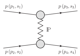
Figure 1: Proton-proton elastic scattering via pomeron exchange.

We shall test three hypotheses for the pomeron and the effective pomeron-proton-proton ($\mathbb{P}pp$) vertex. We shall treat the pomeron either as a scalar, a vector, or a rank-2 symmetric tensor exchange. For all three cases it turns out to be possible to adjust the effective pomeron propagators and the couplings in such a way that at high energies the helicity-conserving $pp$ amplitudes have the standard form as given in the vector-pomeron model due to Donnachie and Landshoff; see [5, 6, 7] and [1]. We will choose the parameters for the scalar and the tensor pomeron accordingly.

2.1 Tensor pomeron $\mathbb{P}_{T}$

Here we describe the pomeron, as discussed in [8], as a symmetric, rank-two, tensor $\mathbb{P}_{T\mu\nu}(x)$ and its interaction with protons by coupling it to a tensor current $J_{T\mu\nu}(x)$,

$$\begin{split}\mathcal{L}^{\prime}_{T}(x)&=J_{T\mu\nu}(x)\,\mathbb{P}_{T}^{\mu\nu}(x)\,,\\ J_{T\mu\nu}(x)&=-3\beta_{\mathbb{P}NN}\frac{i}{2}\bar{\psi}_{p}(x)\left[\gamma_{\mu}\stackrel{{\scriptstyle\leftrightarrow}}{{\partial_{\nu}}}+\gamma_{\nu}\stackrel{{\scriptstyle\leftrightarrow}}{{\partial_{\mu}}}-\frac{1}{2}g_{\mu\nu}\gamma^{\lambda}\stackrel{{\scriptstyle\leftrightarrow}}{{\partial_{\lambda}}}\right]\psi_{p}(x)\,;\end{split}$$ (2.3)

see (6.27) of [8]. Here $\psi_{p}(x)$ is the proton field operator and

$$\begin{split}3\beta_{\mathbb{P}NN}=3\times 1.87\,{\rm GeV}^{-1}\end{split}$$ (2.4)

is the standard coupling constant describing the pomeron-nucleon interaction; see [1, 8]. From (2.3) we get the $\mathbb{P}_{T}pp$ vertex (see (3.43) of [8]) as
                

$$\begin{split}i\Gamma_{\mu\nu}^{(\mathbb{P}_{T}pp)}(p^{\prime},p)=-i\,3\beta_{\mathbb{P}NN}F_{1}[(p^{\prime}-p)^{2}]\left\{\frac{1}{2}\left[\gamma_{\mu}(p^{\prime}+p)_{\nu}+\gamma_{\nu}(p^{\prime}+p)_{\mu}\right]-\frac{1}{4}\,g_{\mu\nu}(\not\!p^{\prime}+\not\!p)\right\}.\end{split}$$ (2.5)

A form factor, $F_{1}(t)$, has been introduced in the vertex (2.5). Conventionally this is taken as the Dirac electromagnetic form factor of the proton, following [5, 6, 7]. The normalisation is

$$\begin{split}F_{1}(0)=1\,.\end{split}$$ (2.6)

In the sequel the precise form of $F_{1}(t)$ will not be relevant.

The ansatz for the effective $\mathbb{P}_{T}$ propagator is given in (3.10) and (3.11) of [8] and reads
                

$$i\Delta^{(\mathbb{P}_{T})}_{\mu\nu,\kappa\lambda}(s,t)=\frac{1}{4s}\left(g_{\mu\kappa}g_{\nu\lambda}+g_{\mu\lambda}g_{\nu\kappa}-\frac{1}{2}g_{\mu\nu}g_{\kappa\lambda}\right)\,(-is\alpha^{\prime}_{\mathbb{P}})^{\alpha_{\mathbb{P}}(t)-1}\,.$$ (2.7)

We assume a standard linear form for the pomeron trajectory (see [1, 8])

$$\begin{split}\alpha_{\mathbb{P}}(t)&=1+\epsilon_{\mathbb{P}}+\alpha^{\prime}_{\mathbb{P}}t\,,\\ \epsilon_{\mathbb{P}}&=0.0808\,,\\ \alpha^{\prime}_{\mathbb{P}}&=0.25\,\mbox{GeV}^{-2}\,.\end{split}$$ (2.8)

2.2 Vector pomeron $\mathbb{P}_{V}$

Here the pomeron has a vector index and is coupled to a vector current

$$\begin{split}\mathcal{L}^{\prime}_{V}(x)&=J_{V\mu}(x)\,\mathbb{P}_{V}^{\mu}(x)\,,\\ J_{V\mu}(x)&=-3\beta_{\mathbb{P}NN}\,M_{0}\,\bar{\psi}_{p}(x)\gamma_{\mu}\psi_{p}(x)\,,\end{split}$$ (2.9)

where $M_{0}\equiv 1$ GeV is introduced for dimensional reasons. The corresponding $\mathbb{P}_{V}pp$ vertex and $\mathbb{P}_{V}$ propagator are as follows (see (B.1) and (B.2) of [9]):
                

$$\begin{split}i\Gamma_{\mu}^{(\mathbb{P}_{V}pp)}(p^{\prime},p)=-i\,3\beta_{\mathbb{P}NN}M_{0}F_{1}[(p^{\prime}-p)^{2}]\,\gamma_{\mu}\,,\end{split}$$ (2.10)

$$\begin{split}i\Delta^{(\mathbb{P}_{V})}_{\mu\nu}(s,t)=\frac{1}{M_{0}^{2}}g_{\mu\nu}\,(-is\alpha^{\prime}_{\mathbb{P}})^{\alpha_{\mathbb{P}}(t)-1}\,.\end{split}$$ (2.11)

2.3 Scalar pomeron $\mathbb{P}_{S}$

Finally, for comparison, we discuss also a scalar pomeron $\mathbb{P}_{S}$ coupled to a scalar current

$$\begin{split}\mathcal{L}^{\prime}_{S}(x)&=J_{S}(x)\,\mathbb{P}_{S}(x)\,,\\ J_{S}(x)&=-3\beta_{\mathbb{P}NN}\,M_{0}\,\bar{\psi}_{p}(x)\psi_{p}(x)\,.\end{split}$$ (2.12)

Here we have as $\mathbb{P}_{S}pp$ coupling and as $\mathbb{P}_{S}$ propagator the following expressions:
                

$$\begin{split}i\Gamma^{(\mathbb{P}_{S}pp)}(p^{\prime},p)=-i\,3\beta_{\mathbb{P}NN}M_{0}F_{1}[(p^{\prime}-p)^{2}]\,,\end{split}$$ (2.13)

$$\begin{split}i\Delta^{(\mathbb{P}_{S})}(s,t)=\frac{s}{2m_{p}^{2}M_{0}^{2}}\,(-is\alpha^{\prime}_{\mathbb{P}})^{\alpha_{\mathbb{P}}(t)-1}\,.\end{split}$$ (2.14)

3 Helicity amplitudes

There are 16 helicity amplitudes for the reaction (2.1), defined as the $\mathcal{T}$-matrix elements

$$\begin{split}\Braket{p(p_{3},s_{3}),p(p_{4},s_{4})}{{\cal T}}{p(p_{1},s_{1}),p(p_{2},s_{2})}&\equiv\Braket{2s_{3},2s_{4}}{{\cal T}}{2s_{1},2s_{2}}\,,\\ \;s_{j}\in\{1/2,-1/2\},&\quad j=1,\dots,4\,.\end{split}$$ (3.1)

The standard references for the general analysis of these amplitudes are [15, 16, 17]; see also [18]. Using rotational, parity ($P$), and time reversal ($T$) invariance, and taking into account that protons are fermions one finds that only five out of the 16 helicity amplitudes (3.1) are independent. Conventionally these are taken as

$$\begin{split}&\phi_{1}(s,t)=\Braket{++}{{\cal T}}{++}\,,\\ &\phi_{2}(s,t)=\Braket{++}{{\cal T}}{--}\,,\\ &\phi_{3}(s,t)=\Braket{+-}{{\cal T}}{+-}\,,\\ &\phi_{4}(s,t)=\Braket{+-}{{\cal T}}{-+}\,,\\ &\phi_{5}(s,t)=\Braket{++}{{\cal T}}{+-}\,.\end{split}$$ (3.2)

The amplitudes with no helicity flip are $\phi_{1}$ and $\phi_{3}$, with single flip $\phi_{5}$, and with double flip $\phi_{2}$ and $\phi_{4}$. Our normalisation is such that the differential cross section for unpolarised protons is

$$\begin{split}\frac{d\sigma(pp\to pp)}{dt}&=\frac{1}{16\pi s(s-4m_{p}^{2})}\frac{1}{4}\sum_{s_{1},\dots,s_{4}}|\Braket{2s_{3},2s_{4}}{{\cal T}}{2s_{1},2s_{2}}|^{2}\\ &=\frac{1}{32\pi}\frac{1}{s(s-4m_{p}^{2})}\left\{|\phi_{1}(s,t)|^{2}+|\phi_{2}(s,t)|^{2}+|\phi_{3}(s,t)|^{2}+|\phi_{4}(s,t)|^{2}\right.\\ &\hskip 96.73918pt\left.+\,4\,|\phi_{5}(s,t)|^{2}\right\}\,.\end{split}$$ (3.3)

The total cross section for unpolarised protons is

$$\begin{split}\sigma_{\rm tot}(pp)&=\frac{1}{\sqrt{s(s-4m_{p}^{2})}}\frac{1}{4}\sum_{s_{1},s_{2}}{\rm Im}\Braket{2s_{1},2s_{2}}{{\cal T}}{2s_{1},2s_{2}}\mid_{t=0}\\ &=\frac{1}{2\sqrt{s(s-4m_{p}^{2})}}\,{\rm Im}\left[\phi_{1}(s,0)+\phi_{3}(s,0)\right]\,.\end{split}$$ (3.4)

Now it is straightforward to calculate the amplitudes $\phi_{j}(s,t)$ in the tensor-, vector-, and scalar-pomeron models of section 2. We use the phase conventions for the proton spinors of definite helicity as given in (4.10) of [15] and find the following results.

Tensor pomeron

$$\begin{split}i\Braket{2s_{3},2s_{4}}{{\cal T}}{2s_{1},2s_{2}}=&\,i\Braket{p(p_{3},s_{3})}{J_{T\mu\nu}(0)}{p(p_{1},s_{1})}i\Delta^{(\mathbb{P}_{T})\mu\nu,\kappa\lambda}(s,t)\\ &{}\times i\Braket{p(p_{4},s_{4})}{J_{T\,\kappa\lambda}(0)}{p(p_{2},s_{2})}\,,\\ \Braket{p(p^{\prime},s^{\prime})}{J_{T\mu\nu}(0)}{p(p,s)}=&\,\bar{u}(p^{\prime},s^{\prime})\,\Gamma^{(\mathbb{P}_{T}pp)}_{\mu\nu}(p^{\prime},p)\,u(p,s)\,.\end{split}$$ (3.5)

Inserting here the expressions from (2.5) and (2.7) we get the amplitudes $\phi_{j}(s,t)$. It is convenient to pull out a common factor

$$\begin{split}{\cal F}(s,t)&=i\left[3\beta_{\mathbb{P}NN}F_{1}(t)\right]^{2}\frac{1}{4s}(-is\alpha^{\prime}_{\mathbb{P}})^{\alpha_{\mathbb{P}}(t)-1}\\ &=\left[3\beta_{\mathbb{P}NN}F_{1}(t)\right]^{2}\frac{1}{4s}(s\alpha^{\prime}_{\mathbb{P}})^{\alpha_{\mathbb{P}}(t)-1}\left[\sin\left(\frac{\pi}{2}({\alpha_{\mathbb{P}}(t)-1})\right)+i\cos\left(\frac{\pi}{2}({\alpha_{\mathbb{P}}(t)-1})\right)\right]\end{split}$$ (3.6)

and to define reduced amplitudes by

$$\begin{split}\hat{\phi}_{j}(s,t)=\phi_{j}(s,t)/{\cal F}(s,t)\,,\qquad j=1,\dots,5.\end{split}$$ (3.7)

The results for $\hat{\phi}_{j}(s,t)$ in the tensor-pomeron model are given in the column ’tensor’ of Table 1. Terms of relative order $m_{p}^{2}/s$ and $|t|/s$ are neglected.

	pomeron ansatz
	tensor	vector	scalar
$\hat{\phi}_{1}(s,t)$	8 $s^{2}$	8 $s^{2}$	8 $s^{2}$
$\hat{\phi}_{2}(s,t)$	10 $m_{p}^{2}t$	16 $m_{p}^{2}t$	2 $s^{2}t/m_{p}^{2}$
$\hat{\phi}_{3}(s,t)$	8 $s^{2}$	8 $s^{2}$	8 $s^{2}$
$\hat{\phi}_{4}(s,t)$	-10 $m_{p}^{2}t$	-16 $m_{p}^{2}t$	-2 $s^{2}t/m_{p}^{2}$
$\hat{\phi}_{5}(s,t)$	-8 $sm_{p}\sqrt{-t}$	-8 $sm_{p}\sqrt{-t}$	-4 $s^{2}\sqrt{-t}/m_{p}$

Table 1: Results for the reduced $pp$ scattering amplitudes $\hat{\phi}_{j}$ (3.7), $j=1,\dots,5$, for the tensor-, vector-, and scalar-pomeron ansätze. Terms of relative order $m_{p}^{2}/s$ and $|t|/s$ are neglected.

Vector pomeron

$$\begin{split}i\Braket{2s_{3},2s_{4}}{{\cal T}}{2s_{1},2s_{2}}=&\,i\Braket{p(p_{3},s_{3})}{J_{V\mu}(0)}{p(p_{1},s_{1})}\;i\Delta^{(\mathbb{P}_{V})\mu\nu}(s,t)\\ &{}\times i\Braket{p(p_{4},s_{4})}{J_{V\nu}(0)}{p(p_{2},s_{2})}\,,\\ \Braket{p(p^{\prime},s^{\prime})}{J_{V\mu}(0)}{p(p,s)}=&\,\bar{u}(p^{\prime},s^{\prime})\,\Gamma^{(\mathbb{P}_{V}pp)}_{\mu}(p^{\prime},p)\,u(p,s)\,.\end{split}$$ (3.8)

Inserting here the expressions from (2.10) and (2.11) we get the reduced amplitudes $\hat{\phi}_{j}(s,t)$ (3.7) in the column ’vector’ of Table 1.

Scalar pomeron

$$\begin{split}i\Braket{2s_{3},2s_{4}}{{\cal T}}{2s_{1},2s_{2}}=&\,i\Braket{p(p_{3},s_{3})}{J_{S}(0)}{p(p_{1},s_{1})}i\Delta^{(\mathbb{P}_{S})}(s,t)\\ &{}\times i\Braket{p(p_{4},s_{4})}{J_{S}(0)}{p(p_{2},s_{2})}\,,\\ \Braket{p(p^{\prime},s^{\prime})}{J_{S}(0)}{p(p,s)}=&\,\bar{u}(p^{\prime},s^{\prime})\,\Gamma^{(\mathbb{P}_{S}pp)}(p^{\prime},p)\,u(p,s)\,.\end{split}$$ (3.9)

Inserting here the expressions from (2.13) and (2.14) we get the reduced amplitudes $\hat{\phi}_{j}(s,t)$ (3.7) in the column ’scalar’ of Table 1.

4 Discussion and comparison with experiment

We note first that, by construction, the non-flip amplitudes $\phi_{1}(s,t)$ and $\phi_{3}(s,t)$ are the same for all three pomeron hypotheses. Thus, from (3.4), we get the same total cross section

$$\begin{split}\sigma_{\rm tot}(pp)=2\left(3\beta_{\mathbb{P}NN}\right)^{2}\cos\left(\frac{\pi}{2}(\alpha_{\mathbb{P}}(0)-1)\right)\left(s\alpha^{\prime}_{\mathbb{P}}\right)^{\alpha_{\mathbb{P}}(0)-1}\,.\end{split}$$ (4.1)

This is the standard expression for the soft-pomeron contribution to $\sigma_{\rm tot}(pp)$; see [1] and (6.41) of [8].

Now we consider the vector-pomeron case. There, big problems arise if we consider $pp$ and $\bar{p}p$ scattering. For $\bar{p}p$ elastic scattering we get an expression analogous to (3.8),

$$\begin{split}&i\Braket{\bar{p}(p_{3},s_{3}),p(p_{4},s_{4})}{{\cal T}}{\bar{p}(p_{1},s_{1}),p(p_{2},s_{2})}\\ &=i\Braket{\bar{p}(p_{3},s_{3})}{J_{V\mu}(0)}{\bar{p}(p_{1},s_{1})}\;i\Delta^{(\mathbb{P}_{V})\mu\nu}(s,t)\;i\Braket{p(p_{4},s_{4})}{J_{V\nu}(0)}{p(p_{2},s_{2})}\,.\end{split}$$ (4.2)

A charge-conjugation transformation $C$ gives

$$\begin{split}\Braket{\bar{p}(p_{3},s_{3})}{J_{V\mu}(0)}{\bar{p}(p_{1},s_{1})}=-\Braket{p(p_{3},s_{3})}{J_{V\mu}(0)}{p(p_{1},s_{1})}\,,\end{split}$$ (4.3)

as follows from the standard $C$-transformation rules of the (anti)proton states and of the bilinear expression for the vector current in terms of the proton fields (2.9). Thus, we get for a vector pomeron

$$\begin{split}&\Braket{\bar{p}(p_{3},s_{3}),p(p_{4},s_{4})}{{\cal T}}{\bar{p}(p_{1},s_{1}),p(p_{2},s_{2})}\\ &\hskip 14.22636pt=-\Braket{p(p_{3},s_{3}),p(p_{4},s_{4})}{{\cal T}}{p(p_{1},s_{1}),p(p_{2},s_{2})}\end{split}$$ (4.4)

and hence from (3.4)

$$\begin{split}\sigma_{\rm tot}(\bar{p}p)=-\sigma_{\rm tot}(pp)\,.\end{split}$$ (4.5)

Clearly, this result does not make sense for a non-vanishing cross section and would contradict the rules of quantum field theory. Thus, we shall not consider a vector pomeron any further.

We are left with the tensor- and scalar-pomeron hypotheses. We note that the $C$ transformation here gives (see (2.3) and (2.12))

$$\begin{split}\Braket{\bar{p}(p_{3},s_{3})}{J_{T\mu\nu}(0)}{\bar{p}(p_{1},s_{1})}=\Braket{p(p_{3},s_{3})}{J_{T\mu\nu}(0)}{p(p_{1},s_{1})}\,,\end{split}$$ (4.6)

and

$$\begin{split}\Braket{\bar{p}(p_{3},s_{3})}{J_{S}(0)}{\bar{p}(p_{1},s_{1})}=\Braket{p(p_{3},s_{3})}{J_{S}(0)}{p(p_{1},s_{1})}\,.\end{split}$$ (4.7)

This implies in both cases the equality of the pomeron contributions to the $pp$ and $\bar{p}p$ scattering amplitudes, as should be the case.

In order to discriminate between the tensor and scalar pomeron cases we turn to data from the STAR experiment at RHIC [14]. There, a measurement of the ratio of single-flip to non-flip amplitudes at $\sqrt{s}=200\,\mbox{GeV}$ was performed. The relevant quantity is

$$\begin{split}r_{5}(s,t)=\frac{2m_{p}\,\phi_{5}(s,t)}{\sqrt{-t}\,{\rm Im}\left[\phi_{1}(s,t)+\phi_{3}(s,t)\right]}\,.\end{split}$$ (4.8)

From (3.6), (3.7) and Table 1 we find for the tensor pomeron

$$\begin{split}r_{5}^{\mathbb{P}_{T}}(s,t)=-\frac{m_{p}^{2}}{s}\left[i+\tan\left(\frac{\pi}{2}(\alpha_{\mathbb{P}}(t)-1)\right)\right]\,.\end{split}$$ (4.9)

For the scalar pomeron, on the other hand, we get

$$\begin{split}r_{5}^{\mathbb{P}_{S}}(s,t)=-\frac{1}{2}\left[i+\tan\left(\frac{\pi}{2}(\alpha_{\mathbb{P}}(t)-1)\right)\right]\,.\end{split}$$ (4.10)

The measurement of $r_{5}$ in [14] is done for $0.003\leqslant|t|\leqslant 0.035$ GeV² and no $t$-dependence of $r_{5}$ is observed in this range. The latter observation is in agreement with our results (4.9) and (4.10) which also imply only a weak $t$-dependence of $r_{5}(s,t)$. Therefore, we can approximately set $t=0$ in (4.9) and (4.10) and obtain with $\sqrt{s}=200\,\mbox{GeV}$

$$r_{5}^{\mathbb{P}_{T}}(s,0)=\left(-0.28-i\,2.20\right)\times 10^{-5}\,,$$ (4.11)

$$r_{5}^{\mathbb{P}_{S}}(s,0)=-0.064-i\,0.500\,.$$ (4.12)

It is worth pointing out that in the high-energy limit ($s\gg m_{p}^{2}$) these results have very small remaining uncertainties since only the pomeron intercept $\alpha_{\mathbb{P}}(0)$ enters which is rather well determined experimentally. However, as the result (4.11) for the tensor pomeron is very small in absolute terms, it is conceivable that in this case subleading terms might be relevant for a calculation of $r_{5}$ with very high precision. But as we will see momentarily, the current experimental uncertainty does not allow a determination of $r_{5}$ to that precision anyway.

In Fig. 2 we show the experimental result for $r_{5}$ of [14] (as given in Fig. 5 there) together with our results (4.11) and (4.12). Clearly, the tensor-pomeron result is perfectly compatible with the experiment. The scalar-pomeron result, on the other hand, is far outside the experimental error ellipse. The tensor pomeron is hence strongly favoured by the data, while the scalar pomeron is ruled out.

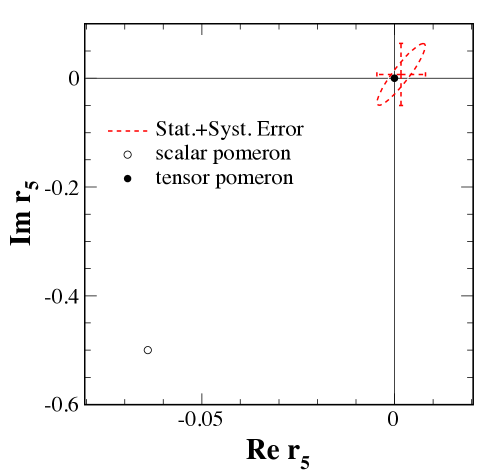
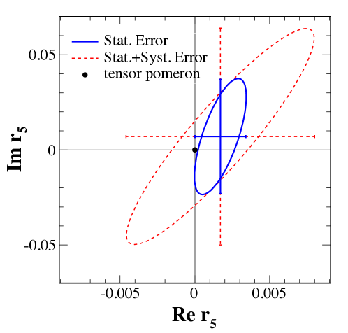
Figure 2: The experimental results for $r_{5}$ at $\sqrt{s}=200\,\mbox{GeV}$ from Fig. 5 of [14] together with our results for the tensor and the scalar pomeron; see (4.11) and (4.12). The first figure shows the experimental data together with the results for both pomeron models. The second figure shows a magnified view of the relevant region around zero and contains only the clearly favoured tensor-pomeron point.

5 Conclusions

In this article we have confronted three hypotheses for the soft pomeron – tensor, vector, and scalar – with experimental data on polarised high-energy $pp$ elastic scattering from the STAR collaboration [14]. Studying the ratio $r_{5}$ of single-helicity-flip to non-flip amplitudes we found that the STAR data are consistent with a tensor pomeron while they clearly exclude a scalar pomeron. We have further argued that a vector pomeron assumption is in contradiction to the rules of quantum field theory. We therefore conclude that the tensor pomeron is the only viable option.

Attempts to relate the pomeron to tensors were, in fact, already discussed in the 1960’s [19, 20, 21]. In [19] the energy-momentum tensor was considered and from that and some further assumptions the ratio of meson-baryon to baryon-baryon cross sections was obtained giving, for instance,

$$\frac{\sigma_{\rm tot}(\pi p)}{\sigma_{\rm tot}(pp)}\approx\frac{m_{K}}{m_{B}}\approx\frac{1}{2}\,.$$ (5.1)

Here $m_{K}$ and $m_{B}$ are a mean meson mass, taken as the one of the $K$ meson, and a mean baryon mass, respectively. This does not work phenomenologically, as in fact $\sigma_{\rm tot}(\pi p)/\sigma_{\rm tot}(pp)\approx 2/3$. Also, we cannot see the physics which would make the $\pi p$ cross section proportional to the $K$ mass.

In this connection we may discuss the consequences of the hypothesis that the tensor current $J_{T\mu\nu}(x)$ in (2.3) is proportional to the energy-momentum tensor with a universal constant of proportionality, independent of the hadron considered. It is easy to see that this leads to the same pomeron part of the total cross section for all hadron-hadron scatterings, for instance $\sigma(pp)=\sigma(\pi p)=\sigma(J/\psi\,p)$. Clearly, also this does not work phenomenologically. Our $J_{T\mu\nu}(x)$ in (2.3) cannot be universally proportional to the energy-momentum tensor.

In [20, 21] attempts were made to relate the pomeron properties, in particular its couplings to hadrons, to those of tensor mesons of the $q\bar{q}$ type. However, with the advent of QCD and gluons it has become clear that the pomeron is a predominantly gluonic object; see the pioneering papers [22, 23]. Thus, if one wants to relate the pomeron properties to mesonic ones it is natural to look for glueballs, and this, indeed, has been and is being done frequently. Here, one problem is that even today the status of glueballs is not particularly clear; for a review see [24]. A vast literature exists dealing with the pomeron in perturbative QCD, starting from the celebrated work [25, 26]. Questions similar to those addressed in the present paper for the soft pomeron could be interesting also in the context of the perturbative pomeron, but this would be beyond the scope of the present paper.

For the soft pomeron phenomenology, for a long time then, a sort of vector pomeron was commonly used, following [5, 6, 7], although it was clear that this could not be completely correct due to the problems with charge conjugation explained in section 4. A first attempt to understand the soft pomeron in the framework of a toy model of nonperturbative QCD was made in [27]. In [28] functional integral techniques were used to analyse high-energy soft hadron-hadron scattering in QCD in a nonperturbative framework. It was shown in chapter 6 of [28] that the pomeron exchange can be understood as a coherent sum of exchanges of spin $2+4+6+\dots$. Going through the arguments there one can see that basically this structure is due to the helicity conserving fundamental quark-gluon coupling in QCD. In [8] a tensor pomeron was introduced which again can be viewed as a coherent sum of exchanges of spin $2+4+6+\dots$ (see appendix B of [8]) thus making contact with the considerations in QCD of [28]. We note that writing a regge exchange as a coherent sum of elementary spin exchanges goes back to [29]. Concerning specific experimental tests for the spin structure of the pomeron we should mention [30] where such tests were proposed for diffractive deep inelastic electron-proton scattering. Similar techniques were proposed in [31, 32] for central production of meson resonances in $pp$ collisions

$$p+p\longrightarrow p+{\rm meson}+p\,.$$ (5.2)

In the light of our discussion here we cannot support the conclusions of [31, 32] that the pomeron couples like a non-conserved vector current. In [9, 11, 12] the question of central production (5.2) was taken up again from the point of view of the tensor pomeron and it was shown that this does quite well in reproducing the data where available. It turned out, however, that central production with pomeron-pomeron fusion,

$$\mathbb{P}+\mathbb{P}\longrightarrow{\rm meson}\,,$$ (5.3)

was not too sensitive to the nature of the pomeron, tensor or vector. But central production with fusion of a $C=-1$ object with the pomeron, e. g.

$$\gamma+\mathbb{P}\longrightarrow\pi^{+}+\pi^{-}$$ (5.4)

is extremely sensitive to the nature of pomeron. For a tensor (vector) pomeron the $\pi^{+}\pi^{-}$ pair in (5.4) is in an antisymmetric (symmetric) state under the exchange $\pi^{+}\leftrightarrow\pi^{-}$. Needless to say that since the pomeron has $C=+1$ the $\pi^{+}\pi^{-}$ pair in (5.4) must be in an antisymmetric state. Thus also from this point, a vector pomeron is excluded. Finally, also investigations of the pomeron using the AdS/CFT correspondence prefer a tensor nature for pomeron exchange [33, 34].

According to the results for the helicity-amplitudes in polarised high-energy $pp$ elastic scattering presented in this work the soft pomeron should be described as a rank-2 symmetric tensor exchange, as for example in the model of [8]. It is not a priori clear that the pomeron exhibits the same spin structure also in reactions involving high momentum transfers, i. e. reactions with the exchange of a hard (perturbative) pomeron. We would find it particularly desirable to study the spin structure of the pomeron in the interesting transition region between soft and hard reactions. It would therefore be useful to discuss further observables that are sensitive to the spin structure of the pomeron and that can be experimentally studied in a wide range of kinematic regimes.

References

- [1] A. Donnachie, H. G. Dosch, P. V. Landshoff, and O. Nachtmann, Pomeron physics and QCD, Camb. Monogr. Part. Phys. Nucl. Phys. Cosmol. 19 (2002).
- [2] L. Caneschi (ed.), Regge Theory of Low Hadronic Interactions, Elsevier Science Publishers B. V., Amsterdam, 1989.
- [3] M. Haguenauer, B. Nicolescu, and J. Tran Thanh Van (eds.), Proceedings of 11th International Conference on Elastic and Diffractive Scattering: Towards High Energy Frontiers, Chateau de Blois, Blois, France, May 2005, The Gioi Publishers, Vietnam, 2006.
- [4] V. Barone and E. Predazzi, High-Energy Particle Diffraction, Springer-Verlag, Berlin, Heidelberg, 2002.
- [5] A. Donnachie and P. V. Landshoff, and Elastic Scattering, Nucl. Phys. B 231 (1984) 189.
- [6] A. Donnachie and P. V. Landshoff, Dynamics of Elastic Scattering, Nucl. Phys. B 267 (1986) 690.
- [7] A. Donnachie and P. V. Landshoff, Hard Diffraction: Production of High Jets, or , and Drell-Yan Pairs, Nucl. Phys. B 303 (1988) 634.
- [8] C. Ewerz, M. Maniatis and O. Nachtmann, A Model for Soft High-Energy Scattering: Tensor Pomeron and Vector Odderon, Annals Phys. 342 (2014) 31 [arXiv:1309.3478 [hep-ph]].
- [9] P. Lebiedowicz, O. Nachtmann and A. Szczurek, Exclusive central diffractive production of scalar and pseudoscalar mesons; tensorial vs. vectorial pomeron, Annals Phys. 344 (2014) 301 [arXiv:1309.3913 [hep-ph]].
- [10] A. Bolz, C. Ewerz, M. Maniatis, O. Nachtmann, M. Sauter and A. Schöning, Photoproduction of pairs in a model with tensor-pomeron and vector-odderon exchange, JHEP 1501 (2015) 151 [arXiv:1409.8483 [hep-ph]].
- [11] P. Lebiedowicz, O. Nachtmann and A. Szczurek, and Drell-Söding contributions to central exclusive production of pairs in proton-proton collisions at high energies, Phys. Rev. D 91 (2015), 074023 [arXiv:1412.3677 [hep-ph]].
- [12] P. Lebiedowicz, O. Nachtmann and A. Szczurek, Central exclusive diffractive production of the continuum, scalar and tensor resonances in and scattering within the tensor pomeron approach, Phys. Rev. D 93 (2016), 054015 [arXiv:1601.04537 [hep-ph]].
- [13] P. Lebiedowicz, O. Nachtmann and A. Szczurek, Exclusive diffractive production of via the intermediate and states in proton-proton collisions within tensor pomeron approach, arXiv:1606.05126 [hep-ph].
- [14] L. Adamczyk et al. [STAR Collaboration], Single Spin Asymmetry in Polarized Proton-Proton Elastic Scattering at GeV, Phys. Lett. B 719 (2013) 62 [arXiv:1206.1928 [nucl-ex]].
- [15] M. L. Goldberger, M. T. Grisaru, S. W. MacDowell and D. Y. Wong, Theory of low-energy nucleon-nucleon scattering, Phys. Rev. 120 (1960) 2250.
- [16] N. H. Buttimore, E. Gotsman and E. Leader, Spin-dependent phenomena induced by electromagnetic-hadronic interference at high energies, Phys. Rev. D 18 (1978) 694.
- [17] N. H. Buttimore, B. Z. Kopeliovich, E. Leader, J. Soffer and T. L. Trueman, Spin dependence of high energy proton scattering, Phys. Rev. D 59 (1999) 114010 [hep-ph/9901339].
- [18] E. Leader, Spin in particle physics, Camb. Monogr. Part. Phys. Nucl. Phys. Cosmol. 15 (2001)
- [19] P. G. O. Freund, “Universality” and high energy total cross sections, Phys. Lett. 2 (1962) 136.
- [20] P. G. O. Freund, Tensor-meson dominance and regge couplings, Nuovo Cim. A 5 (1971) 9.
- [21] R. D. Carlitz, M. B. Green and A. Zee, A model for pomeranchukon couplings, Phys. Rev. Lett. 26 (1971) 1515.
- [22] F. E. Low, A Model of the Bare Pomeron, Phys. Rev. D 12 (1975) 163.
- [23] S. Nussinov, Colored Quark Version of Some Hadronic Puzzles, Phys. Rev. Lett. 34 (1975) 1286.
- [24] W. Ochs, The Status of Glueballs, J. Phys. G 40 (2013) 043001 [arXiv:1301.5183 [hep-ph]].
- [25] E. A. Kuraev, L. N. Lipatov and V. S. Fadin, The Pomeranchuk Singularity in Nonabelian Gauge Theories, Sov. Phys. JETP 45 (1977) 199 [Zh. Eksp. Teor. Fiz. 72 (1977) 377].
- [26] I. I. Balitsky and L. N. Lipatov, The Pomeranchuk Singularity in Quantum Chromodynamics, Sov. J. Nucl. Phys. 28 (1978) 822 [Yad. Fiz. 28 (1978) 1597].
- [27] P. V. Landshoff and O. Nachtmann, Vacuum Structure and Diffraction Scattering, Z. Phys. C 35 (1987) 405.
- [28] O. Nachtmann, Considerations concerning diffraction scattering in quantum chromodynamics, Annals Phys. 209 (1991) 436.
- [29] L. van Hove, Regge pole and single particle exchange mechanisms in high energy collisions, Phys. Lett. 24 (1967) 183.
- [30] T. Arens, O. Nachtmann, M. Diehl and P. V. Landshoff, Some tests for the helicity structure of the pomeron in collisions, Z. Phys. C 74 (1997) 651 [hep-ph/9605376].
- [31] F. E. Close and G. A. Schuler, Central production of mesons: Exotic states versus pomeron structure, Phys. Lett. B 458 (1999) 127 [hep-ph/9902243].
- [32] F. E. Close and G. A. Schuler, Evidence that the pomeron transforms as a nonconserved vector current, Phys. Lett. B 464 (1999) 279 [hep-ph/9905305].
- [33] S. K. Domokos, J. A. Harvey and N. Mann, The Pomeron contribution to and scattering in AdS/QCD, Phys. Rev. D 80 (2009) 126015 [arXiv:0907.1084 [hep-ph]].
- [34] I. Iatrakis, A. Ramamurti and E. Shuryak, Pomeron Interactions from the Einstein-Hilbert Action, arXiv:1602.05014 [hep-ph].