Exact gradient updates in time independent of output size for the spherical loss family

Abstract

An important class of problems involves training deep neural networks with sparse prediction targets of very high dimension $D$. These occur naturally in e.g. neural language models or the learning of word-embeddings, often posed as predicting the probability of next words among a vocabulary of size $D$ (e.g. $200\,000$). Computing the equally large, but typically non-sparse $D$-dimensional output vector from a last hidden layer of reasonable dimension $d$ (e.g. $500$) incurs a prohibitive $O(Dd)$ computational cost for each example, as does updating the $D\times d$ output weight matrix and computing the gradient needed for backpropagation to previous layers. While efficient handling of large sparse network inputs is trivial, the case of large sparse targets is not, and has thus so far been sidestepped with approximate alternatives such as hierarchical softmax or sampling-based approximations during training. In this work we develop an original algorithmic approach which, for a family of loss functions that includes squared error and spherical softmax, can compute the exact loss, gradient update for the output weights, and gradient for backpropagation, all in $O(d^{2})$ per example instead of $O(Dd)$, remarkably without ever computing the $D$-dimensional output. The proposed algorithm yields a speedup of $\frac{D}{4d}$, i.e. two orders of magnitude for typical sizes, for that critical part of the computations that often dominates the training time in this kind of network architecture.

1 Introduction

Many modern applications of neural networks have to deal with data represented, or representable, as very large sparse vectors. Such representations arise in natural language related tasks, where the dimension $D$ of that vector is typically (a multiple of) the size of the vocabulary, but also in the sparse user-item matrices of collaborative-filtering applications. It is trivial to handle very large sparse inputs to a neural network in a computationally efficient manner: the forward propagation and update to the input weight matrix after backpropagation are correspondingly sparse. By contrast, training with very large sparse prediction targets is problematic: even if the target is sparse, the computation of the equally large network output and the corresponding gradient update to the huge output weight matrix are not sparse and thus computationally prohibitive. This has been a practical problem ever since Bengio et al. [1] first proposed using a neural network for learning a language model, in which case the computed output vector represents the probability of the next word and is the size of the considered vocabulary, which is becoming increasingly large in modern applications [2]. Several approaches have been proposed to attempt to address this difficulty essentially by sidestepping it. They fall in two categories:

• Sampling or selection based approximations consider and compute only a tiny fraction of the output’s dimensions sampled at random or heuristically chosen. The reconstruction sampling of Dauphin et al. [3], the efficient use of biased importance sampling in Jean et al. [4], the use of Noise Contrastive Estimation [5] in Mnih and Kavukcuoglu [6] and Mikolov et al. [7] all fall under this category. As does the more recent use of approximate Maximum Inner Product Search based on Locality Sensitive Hashing techniques[8, 9] to select a good candidate subset.

• Hierarchical softmax [10, 7] imposes a heuristically defined hierarchical tree structure for the computation of the normalized probability of the target class.

Compared to the initial problem of considering all $D$ output dimensions, both kinds of approaches are crude approximations. In the present work, we will instead investigate a way to actually perform the exact gradient update that corresponds to considering all $D$ outputs, but do so implicitly, in a computationally efficient manner, without actually computing the $D$ outputs. This approach works for a relatively restricted class of loss functions, that we call the spherical family, its simplest member being linear output with squared error (a natural choice for sparse real-valued regression targets). For simplicity and clarity we will begin with this squared error case, presenting the computational challenge that arises in the standard naive approach in Section 2 and deriving our algorithmic solution in Section 3. We will then extend our approach to the more general case of loss functions in the spherical family in Section 4. In Section 5 we will discuss numerical stability issues that may arise and detail our numerical stabilization strategy. Section 6 presents experimental validation focusing on timings obtained with our CPU and GPU implementations of our algorithm relative to the naive update algorithm.

2 The problem

2.1 Problem definition and setup

We are concerned with gradient-descent based training of a deep feed-forward neural network with target vectors of very high dimension $D$ (e.g. $D=200\,000$) but that are sparse, i.e. a comparatively small number, at most $K\ll D$, of the elements of the target vector are non-zero. Such a $K$-sparse vector will typically be stored and represented compactly as $2K$ numbers corresponding to pairs (index, value). A network to be trained with such targets will naturally have an equally large output layer of dimension $D$. We can also optionally allow the input to the network to be a similarly high dimensional sparse vector of dimension $D_{in}$. Between the large sparse target, output, and (optionally large sparse) input, we suppose the network’s intermediate hidden layers to be of smaller, more typically manageable, dimension $d\ll D$ (e.g. $d=500$).

Mathematical notation:

• Vectors are denoted using lower-case letters, e.g. $h$, and are considered column-vectors; corresponding row vectors are denoted with a transpose, e.g. $h^{T}$.

• Matrices are denoted using upper-case letters, e.g. $W$, with $W^{T}$ the transpose of $W$.

• The $j^{th}$ column of $W$ is denoted $W_{j}$ , and its $i^{th}$ row $W_{i\bullet}$ (both viewed as a column vector).

• $U^{-T}=\left(U^{-1}\right)^{T}$ denotes the transpose of the inverse of a square matrix.

• $\mathbf{1}_{D}$ denotes a $D$-dimensional column vector filled with ones.

• $\mathbf{1}_{i\in\mathcal{A}(y)}$ denotes an indicator function whose value will be 1 if $i\in\mathcal{A}(y)$ and 0 otherwise.

• $\mathrm{onehot}_{D}(j)=\left\{\mathbf{1}_{i=j}\right\}_{i=1}^{D}$ is the $D$-dimensional column vector filled with zeros except at index $j$ where its value is 1.

• $\mathbf{I}_{d}$ is the $d\times d$ identity matrix.

Network architecture

We consider a standard feed forward neural network architecture as depicted in Figure 1. An input vector $x\in\mathbb{R}^{D_{in}}$ is linearly transformed into a linear activation $a^{(1)}=W^{(1)T}x+b^{(1)}$ through a $D_{in}\times d$ input weight matrix $W^{(1)}$ (and an optional bias vector $b^{(1)}\in\mathbb{R}^{d}$). This is typically followed by a non-linear transformation $s$ to yield the representation of the first hidden layer $h^{(1)}=s(a^{(1)})$. This first hidden layer representation is then similarly transformed through a number of subsequent non-linear layers (that can be of any usual kind amenable to backpropagation) e.g. $h^{(k)}=s(a^{(k)})$ with $a^{(k)}=W^{(k)T}h^{(k-1)}+b^{(k)}$ until we obtain last hidden layer representation $h=h^{(m)}$. We then obtain the final $D$-dimensional network output as $o=Wh$ where $W$ is a $D\times d$ output weight matrix, which will be our main focus in this work. Finally, the network’s $D$-dimensional output $o$ is compared to the $D$-dimensional target vector $y$ associated with input $x$ using squared error, yielding loss $L=\|o-y\|^{2}$.

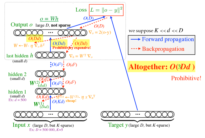
Figure 1: The computational problem posed by very large sparse targets. Dealing with sparse input efficiently is trivial, with both the forward and backward propagation phases easily achieved in $O(Kd)$. However this is not the case with large sparse targets. They incur a prohibitive computational cost of $O(Dd)$ at the output layer as forward propagation, gradient backpropagation and weight update each require accessing all $D\times d$ elements of the large output weight matrix.

Training procedure

This architecture is a typical (possibly deep) multi-layer feed forward neural network architecture with a linear output layer and squared error loss. Its parameters (weight matrices and bias vectors) will be trained by gradient descent, using gradient backpropagation Rumelhart et al. [11], LeCun [12, 13] to efficiently compute the gradients. The procedure is shown in Figure 1. Given an example from the training set as an (input,target) pair $(x,y)$, a pass of forward propagation proceeds as outlined above, computing the hidden representation of each hidden layer in turn based on the previous one, and finally the network’s predicted output $o$ and associated loss $L$. A pass of gradient backpropagation then works in the opposite direction, starting from $\nabla_{o}=\frac{\partial L}{\partial o}=2(o-y)$ and propagating back the gradients $\nabla_{h^{(k)}}=\frac{\partial L}{\partial h^{(k)}}$ and $\nabla_{a^{(k)}}=\frac{\partial L}{\partial a^{(k)}}$ upstream through the network. The corresponding gradient contributions on parameters (weights and biases), collected along the way, are straightforward once we have the associated $\nabla_{a^{(k)}}$. Specifically they are $\nabla_{b^{(k)}}=\nabla_{a^{(k)}}$ and $\nabla_{W^{(k)}}=h^{(k-1)}(\nabla_{a^{(k)}})^{T}$. Similarly for the input layer $\nabla_{W^{(1)}}=x(\nabla_{a^{(1)}})^{T}$, and for the output layer $\nabla_{W}=(o-y)h^{T}$ . Parameters are then updated through a gradient descent step $W^{(k)}\leftarrow W^{(k)}-\eta\nabla_{W^{(k)}}$ and $b^{(k)}\leftarrow b^{(k)}-\eta\nabla_{b^{(k)}}$, where $\eta$ is a positive learning-rate. Similarly for the output layer which will be our main focus here: $W\leftarrow W-\eta\nabla_{W}$.

2.2 The easy part: input layer forward propagation and weight update

It is easy and straightforward to efficiently compute the forward propagation, and the backpropagation and weight update part for the input layer when we have a very large $D_{in}$-dimensional but $K-$sparse input vector $x$ with appropriate sparse representation. Specifically we suppose that $x$ is represented as a pair of vectors $u,v$ of length (at most) $K$, where $u$ contains integer indexes and $v$ the associated real values of the elements of $x$ such that $x_{i}=0$ if $i\notin u$, and $x_{u_{k}}=v_{k}$.

• Forward propagation through the input layer: The sparse representation of $x$ as the positions of $K$ elements together with their value makes it cheap to compute $W^{(1)T}x$. Even though $W^{(1)}$ may be a huge full $D_{in}\times d$ matrix, only $K$ of its rows (those corresponding to the non-zero entries of $x$) need to be visited and summed to compute $W^{(1)T}x$. Precisely, with our $(u,v)$ sparse representation of $x$ this operation can be written as$W^{(1)T}x=\sum_{k=1}^{K}v_{k}W_{:u_{k}}^{(1)}$where each $W_{:u_{k}}^{(1)}$ is a $d$-dimensional vector, making this an $O(Kd)$ operation rather than $O(Dd)$.

• Gradient and update through input layer: Let us for now suppose that we were able to get gradients (through backpropagation) up to the first hidden layer activations $a^{(1)}\in\mathbb{R}^{d}$ in the form of gradient vector $\nabla_{a^{(1)}}=\frac{\partial L}{\partial a^{(1)}}$. The corresponding gradient-based update to input layer weights $W^{(1)}$ is simply $W^{(1)}\leftarrow W^{(1)}-\eta x(\nabla_{a^{(1)}})^{T}$. This is a rank-one update to $W^{(1)}$. Here again, we see that only the $K$ rows of $W^{(1)}$ associated to the (at most) $K$ non-zero entries of $x$ need to be modified. Precisely this operation can be written as:$W_{:u_{k}}^{(1)}\leftarrow W_{:u_{k}}^{(1)}-\eta v_{k}\nabla_{a^{(1)}}\,\,\,\forall k\in\{1,\ldots,K\}$ making this again a $O(Kd)$ operation rather than $O(Dd)$.

2.3 The hard part: output layer propagation and weight update

Given some network input $x$ we suppose we can compute without difficulty through forward propagation the associated last hidden layer representation $h\in\mathbb{R}^{d}$. From then on:

• Computing the final output $o=Wh$ incurs a prohibitive computational cost of $O(Dd)$ since $W$ is a full $D\times d$ matrix. Note that there is a-priori no reason for representation $h$ to be sparse (e.g. with a sigmoid non-linearity) but even if it was, this would not fundamentally change the problem since it is $D$ that is extremely large, and we supposed $d$ reasonably sized already. Computing the residual $(\mbox{o}-y)$ and associated squared error loss $\|\mbox{o}-y\|^{2}$ incurs an additional $O(D)$ cost.

• The gradient on $h$ that we need to backpropagate to lower layers is $\nabla_{h}=\frac{\partial L}{\partial h}=2W^{T}(o-y)$ which is another $O(Dd)$ matrix-vector product.

• Finally, when performing the corresponding output weight update $W\leftarrow W-\eta(o-y)h^{T}$ we see that it is a rank-one update that updates all $D\times d$ elements of $W$, which again incurs a prohibitive $O(Dd)$ computational cost.

For very large $D$, all these three $O(Dd)$ operations are prohibitive, and the fact that $y$ is sparse, seen from this perspective, doesn’t help, since neither $o$ nor $o-y$ will be sparse.

3 A computationally efficient algorithm for performing the exact online gradient update

Previously proposed workarounds are approximate or use stochastic sampling. We propose a different approach that results in the exact same, yet efficient gradient update, remarkably without ever having to compute large output $o$.

3.1 Computing the squared error loss $L$ and the gradient with respect to $h$ efficiently

Suppose that, we have, for a network input example $x$, computed the last hidden representation $h\in\mathbb{R}^{d}$ through forward propagation. The network’s $D$ dimensional output $o=Wh$ is then in principle compared to the high dimensional target $y\in\mathbb{R}^{D}$. The corresponding squared error loss is $L=\left\|Wh-y\right\|^{2}$. As we saw in Section 2.3, computing it in the direct naive way would have a prohibitive computational complexity of $O(Dd+D)=O(Dd)$ because computing output $Wh$ with a full $D\times d$ matrix $W$ and a typically non-sparse $h$ is $O(Dd)$. Similarly, to backpropagate the gradient through the network, we need to compute the gradient of loss $L$ with respect to last hidden layer representation $h$. This is $\nabla_{h}=\frac{\partial L}{\partial h}=\frac{\partial\left\|Wh-y\right\|^{2}}{\partial h}=2W^{T}(Wh-y)$. So again, if we were to compute it directly in this manner, the computational complexity would be a prohibitive $O(Dd)$. Provided we have maintained an up-to-date matrix $Q=W^{T}W$, which is of reasonable size $d\times d$ and can be cheaply maintained as we will see in Section 3.4, we can rewrite these two operations so as to perform them in $O(d^{2})$:

Loss computation:

$$L = \|\overbrace{Wh}^{O(Dd)}-y\|^{2}$$ (1)

$$= \left(Wh-y\right)^{T}\left(Wh-y\right)$$

$$= h^{T}W^{T}Wh-y^{T}Wh-h^{T}W^{T}y+y^{T}y$$

$$= h^{T}Qh-2h^{T}(W^{T}y)+y^{T}y$$

$$= h^{T}(\underbrace{Qh}_{O(d^{2})}-2\underbrace{W^{T}y}_{O(Kd)})+\underbrace{y^{T}y}_{O(K)}$$

Gradient on $h$:

$$\nabla_{h}=\frac{\partial L}{\partial h} = \frac{\partial\|Wh-y\|^{2}}{\partial h}$$ (2)

$$= 2W^{T}(Wh-y)$$

$$= 2\left(W^{T}Wh-W^{T}y\right)$$

$$= 2(\underbrace{Qh}_{O(d^{2})}-\underbrace{W^{T}y}_{O(Kd)})$$

The terms in $O(Kd)$ and $O(K)$ are due to leveraging the $K$-sparse representation of target vector $y$. With $K\ll D$ and $d\ll D$, we get altogether a computational cost of $O(d^{2})$ which can be several orders of magnitude cheaper than the prohibitive $O(Dd)$ of the direct approach.

3.2 Efficient gradient update of $W$

The gradient of the squared error loss with respect to output layer weight matrix $W$ is $\frac{\partial L}{\partial W}=\frac{\partial\left\|Wh-y\right\|^{2}}{\partial W}=2(Wh-y)h^{T}$. And the corresponding gradient descent update to $W$ would be $W_{new}\leftarrow W-2\eta(Wh-y)h^{T}$, where $\eta$ is a positive learning rate. Again, computed in this manner, this induces a prohibitive $O(Dd)$ computational complexity, both to compute output and residual $Wh-y$, and then to update all the $Dd$ elements of $W$ (since generally neither $Wh-y$ nor $h$ will be sparse). All $D\times d$ elements of $W$ must be accessed during this update. On the surface this seems hopeless. But we will now see how we can achieve the exact same update on $W$ in $O(d^{2})$. The trick is to represent $W$ implicitly as the factorization $\underbrace{W}_{D\times d}=\underbrace{V}_{D\times d}\underbrace{U}_{d\times d}$and update $U$ and $V$ instead:

$$\mathbf{a)}\,\,U_{new} = U-2\eta(Uh)h^{T}$$ (3)

$$\mathbf{b)}\,\,V_{new} = V+2\eta y(U_{new}^{-T}h){}^{T}$$ (4)

This results in implicitly updating $W$ as we did explicitly in the naive approach as we now prove:

$$V_{new}U_{new} = (V+2\eta y(U_{new}^{-T}h){}^{T})\,U_{new}$$

$$= VU_{new}+2\eta y(U_{new}^{-T}h){}^{T}U_{new}$$

$$= VU_{new}+2\eta yh^{T}U_{new}^{-1}U_{new}$$

$$= V(U-2\eta(Uh)h^{T})+2\eta yh^{T}(U_{new}^{-1}U_{new})$$

$$= VU-2\eta VUhh^{T}+2\eta yh^{T}$$

$$= VU-2\eta(VUh-y)h^{T}$$

$$= W-2\eta(Wh-y)^{T}h^{T}$$

$$= W_{new}$$

We see that the update of $U$ in Eq. 3 is a simple $O(d^{2})$ operation. Following this simple rank-one update to $U$, we can use the Sherman-Morrison formula to derive the corresponding rank-one update to $U^{-T}$ which will also be $O(d^{2})$:

$$U_{new}^{-T} = U^{-T}+\frac{2\eta}{1-2\eta\left\|h\right\|^{2}}(U^{-T}h)h^{T}$$ (5)

It is then easy to compute the $U_{new}^{-T}h$, an $O(d^{2})$ operation needed in Eq. 4. The ensuing rank-one update of $V$ in Eq 4, thanks to the $K$-sparsity of $y$ is only $O(Kd)$: only the$K$ rows $V$ associated to non-zero elements in $y$ are accessed and updated, sited of all $D$ rows of $W$ we had to modify in the naive update!

3.3 Adapting the computation of $L$ and $\nabla_{h}$ to the factored representation of $W$

With the factored representation of $W$ as $VU$, we only have $W$ implicitly, so the $W^{T}y$ terms that entered in the computation of $L$ and $\nabla_{h}$ in the previous section (Eq. 1 and 2) need to be adapted slightly as $\hat{y}=W^{T}y=U^{T}(V^{T}y)$, which becomes $O(d^{2}+Kd)$ rather than $O(Kd)$ in computational complexity. But this doesn’t change the overall $O(d^{2})$ complexity of these computations.

The adapted update computation of $L$ and $\nabla_{h}$ can thus be expressed simply as:

$$\nabla_{h}=2\underbrace{(\underbrace{Qh}_{\hat{h}}-\underbrace{U^{T}(V^{T}y)}_{\hat{y}})}_{\hat{z}}$$ (6)

and

$$L=h^{T}(\underbrace{Qh}_{\hat{h}}-2\underbrace{U^{T}(V^{T}y)}_{\hat{y}})+y^{T}y$$ (7)

3.4 Bookkeeping: keeping an up-to-date $Q$ and $U^{-T}$

We have already seen, in Eq. 5, how we can cheaply maintain an up-to-date $U^{-T}$ following our update of $U$. Similarly, following our updates to $U$ and $V$, we need to keep an up-to-date $Q=W^{T}W$ which is needed to efficiently compute the loss $L$ (Eq. 1) and gradient $\nabla_{h}$ (Eq. 2). We have shown that updates to $U$ and $V$ in equations 3 and 4 are equivalent to implicitly updating $W$ as $W_{new}\leftarrow W-2\eta(Wh-y)h^{T}$, and this translates into the following update to $Q=W^{T}W$:

$$Q_{new} = Q-\eta\left(h\nabla_{h}^{T}+\nabla_{h}h^{T}\right)+(4\eta^{2}L)hh^{T}$$ (8)

One can see that this last bookkeeping operation also has a $O(d^{2})$ computational complexity.

Proof that this update to $Q$ corresponds to the update $W_{new}\leftarrow 2(Wh-y)h^{T}$

$$W_{new}^{T}W_{new} = \left(W-2\eta(Wh-y)h^{T}\right)^{T}\left(W-2\eta(Wh-y)h^{T}\right)$$

$$W_{new}^{T}W_{new} = W^{T}W-2\eta h(Wh-y)^{T}W-2\eta W^{T}(Wh-y)h^{T}$$

$$+4\eta^{2}h(Wh-y)^{T}(Wh-y)h^{T}$$

$$W_{new}^{T}W_{new} = Q-2\eta\left(hh^{T}W^{T}W-hy^{T}W\right)-2\eta\left(W^{T}Whh^{T}-W^{T}yh^{T}\right)$$

$$+4\eta^{2}h(h^{T}W^{T}Wh-h^{T}W^{T}y-y^{T}Wh+y^{T}y)h^{T}$$

$$W_{new}^{T}W_{new} = Q-2\eta\left(hh^{T}Q-h(W^{T}y)^{T}\right)-2\eta\left(Qhh^{T}-(W^{T}y)h^{T}\right)$$

$$+4\eta^{2}h(h^{T}Qh-h^{T}(W^{T}y)-(W^{T}y)^{T}h+y^{T}y)h^{T}$$

$$W_{new}^{T}W_{new} = Q-2\eta h\left(h^{T}Q-(W^{T}y)^{T}\right)-2\eta\left(Qh-W^{T}y\right)h^{T}$$

$$+4\eta^{2}h(h^{T}Qh-2h^{T}W^{T}y+y^{T}y)h^{T}$$

$$W_{new}^{T}W_{new} = Q-\eta h(\underbrace{2(Qh-W^{T}y)}_{\nabla_{h}})^{T}-\eta(\underbrace{2(Qh-W^{T}y)}_{\nabla_{h}})h^{T}$$

$$+4\eta^{2}h\underbrace{(h^{T}(Qh-2W^{T}y)+y^{T}y)}_{L}h^{T}$$

where we see that the last term uses the expression of $L$ from Eq. 1 and the first two terms uses the expression of $\nabla_{h}$ from Eq. 6: $\nabla_{h}=2(Qh-U^{T}(V^{T}y))=2(Qh-W^{T}y)$. Thus we have shown that

$$W_{new}^{T}W_{new} = Q-\eta h\nabla_{h}^{T}-2\eta\nabla_{h}h^{T}+4\eta^{2}hLh^{T}$$

$$= Q-\eta\left(h\nabla_{h}^{T}+\nabla_{h}h^{T}\right)+(4\eta^{2}L)hh^{T}$$

which is the update $Q_{new}$ that we gave in Eq. 8 above.

3.5 Putting it all together: detailed online update algorithm and expected benefits

We have seen that we can efficiently compute cost $L$, gradient with respect to $h$ (to be later backpropagated further) as well as updating $U$ and $V$ and performing the bookkeeping for $U^{-T}$ and $Q$. Here we put everything together. The parameters of the output layer that we will learn are $V,U$ and implicitly represent $W$ as $W=VU$. We first need to initialize these parameter matrices, as well as bookkeeping matrices $Q$ and $U^{-T}$ in a consistent way, as explained in Algo. 1. We then iterate over the following:

• pick a next input,target example $x,y$ (where $y$ is $K$-sparse and uses an appropriate sparse representation)

• perform forward propagation through all layers of the network up to the last hidden layer, to compute last hidden layer representation $h=h(x)$, that should include a constant 1 first element.

• execute Algo. 2, that we put together from the equations derived above, and that will: compute the associated squared error loss $L$, perform an implicit gradient update step on $W$ by correspondingly updating $V$ and $U$ in a computationally efficient manner, update bookkeeping matrices $Q$ and $U^{-T}$ accordingly, and compute and return the gradient of the loss with respect to the last hidden layer $\nabla_{h}$

• having $\nabla_{h}$, further backpropagate the gradients upstream, and use them to update the parameters of all other layers

Having $K\ll d\ll D$ we see that the update algorithm we developed requires $O(d^{2})$ operations, whereas the standard approach required $O(Dd)$ operations. If we take $K\approx d$ , we may state more precisely that the proposed algorithm, for computing the loss and the gradient updates will require roughly $12d^{2}$ operations whereas the standard approach required roughly $3Dd$ operations. So overall the proposed algorithm change corresponds to a computational speedup by a factor of $\frac{D}{4d}$. For $D=200\,000$ and $d=500$ the expected speedup is thus 100. Note that the advantage is not only in computational complexity, but also in memory access. For each example, the standard approach needs to access and change all $D\times d$ elements of matrix $W$, whereas the proposed approach only accesses the much smaller number $K\times d$ elements of $V$ as well as the three $d\times d$ matrices $U$, $U^{-T}$, and $Q$. So overall we have a substantially faster algorithm whose complexity is independent of $D$, which, while doing so implicitly, will nevertheless perform the exact same gradient update as the standard $O(Dd)$ approach. We want to emphasize here that this approach is entirely different from simply chaining 2 linear layers $U$ and $V$ and performing ordinary gradient descent updates on these: this would result in the same prohibitive computational complexity as the standard approach, and such ordinary separate gradient updates to $U$ and $V$ would not be equivalent to the ordinary gradient update to $W=VU$.

Algorithm 1 Initialization of output layer parameters $V,U$ and bookkeeping matrices $Q,U^{-T}$

• we can initialize $D\times d$ matrix $V$ randomly as we would have initialized $W$ so that we initially have $V=W$.
  Alternatively we can initialize $V$ to 0 (there won’t be symmetry breaking issues with having $W$ initially be 0 provided the other layers are initialized randomly, since varying inputs and targets will naturally break symmetry for the output layer)

• initialize $Q\leftarrow V^{T}V$ (or more cheaply initialize $Q\leftarrow 0$ if we have initialized $V$ to 0).

• we initialize $U$ to the identity: $U\leftarrow\mathbf{I}_{d}$ so that, trivially, we initially have $VU=W$.

• initialize $U^{-T}\leftarrow\mathbf{I}_{d}$

Algorithm 2 Efficient computation of cost $L$, gradient $\nabla h$, and update to parameters $U$ and $V$ for squared error, in the online case

Inputs (besides above parameters $V,U,Q,U^{-T}$):

• $h\in\mathbb{R}^{d}$ hidden representation vector for one example $h\in\mathbb{R}^{d}$

• $y\in\mathbb{R}^{D}$ associated K-sparse target vector stored using a sparse representation (indices and values of non-zero elements)

• $\eta\in\mathbb{R}^{+}$learning rate for the update

Outputs:

• $L\in\mathbb{R}$ the squared error loss for this example

• updated parameters and bookkeeping matrices $U_{new},V_{new},Q_{new},U_{new}^{-T}$

• $\nabla_{h}\in\mathbb{R}^{d}$ the gradient of the loss with respect to $h$, to further backpropagate upstream.

Algorithm:

Step #	Operation	Computational complexity	Approximate number of elementary operations (multiply-adds)
1:	$\hat{h}=Qh$	$O(d^{2})$	$d^{2}$
2:	$\hat{y}=U^{T}(V^{T}y)$	$O(Kd+d^{2})$	$Kd+d^{2}$
3:	$\nabla_{h}=2(\hat{h}-\hat{y})$	$O(d)$	$d$
4:	$L=h^{T}\hat{h}-2h^{T}\hat{y}+y^{T}y$	$O(2d+K)$	$2d+K+1$
5:	$U\leftarrow U-2\eta(Uh)h^{T}$	$O(d^{2})$	$2d^{2}+d$
6:	$U^{-T}\leftarrow U^{-T}+\frac{2\eta}{1-2\eta\left\|h\right\|^{2}}(U^{-T}h)h^{T}$ [ from Sherman-Morrison formula ]	$O(d^{2})$	$2d^{2}+2d+3$
7:	$V\leftarrow V+2\eta y(U^{-T}h){}^{T}$ where we must use the freshly updated $U^{-T}$ resulting from step 6)	$O(d^{2}+Kd)$	$d^{2}+K+Kd$
8:	$Q\leftarrow Q-\eta\left(h\nabla_{h}^{T}+\nabla_{h}h^{T}\right)+(4\eta^{2}L)hh^{T}$	$O(d^{2})$	$4+2d+3d^{2}$
	Altogether:	$O(d^{2})$ provided $K<d\ll D$	$\approx 12d^{2}$ elementary operations

3.6 Minibatch version of the algorithm for squared error

The algorithm we derived for online gradient is relatively straightforward to extend to the case of minibatches containing $m$ examples. We iniialize parameters as in the online case follpwing Algo. 1 and apply the same training procedure outlined in Section. 3.5, but now using minibatches containing $m$ examples, rather than a single example vector. The corresponding update and gradient computation is given in Algorithm  3 which follows equivalent steps to the online version of Algorithm 2, but using matrices with $m$ columns in place of single column vectors. For example step 3 which in the online algorithm was $\nabla_{h}=2(\hat{h}-\hat{y})$ using $d-$dimensional vectors becomes in the minibatch version $\nabla_{H}=2(\hat{H}-\hat{Y})$ using $d\times m$ matrices instead.

Note that in the minibatch version, in step 6, we update $U^{-T}$ based on the Woodbury equation, which generalizes the Sheman-Morrison formula for $m>1$ and involves inverting an $m\times m$ matrix, an $O(m^{3})$ operation. But depending on the size of the minibatch $m$, it may become more efficient to solve the corresponding linear equations for each minibatch from scratch every time, rather than inverting that $m\times m$ matrix. In which case we won’t need to maintain an $U^{-T}$ at all. Or in cases of minibatches containing more than $d$ examples, it may even become more efficient to invert $U$ from scratch every time.

In step 9, the update $Q_{new}$ for $Q$ corresponds to the implicit weight update $W_{new}\leftarrow W-2\eta(WH-Y)H^{T}$ as we now prove:

We will use the following precomputed quantities: $Q=W^{T}W$, $\hat{H}=QH$ and $\hat{Y}=W^{T}Y=U^{T}(V^{T}Y)$ and $\nabla_{H}=2(\hat{H}-\hat{Y})$.

$$Q_{new} = W_{new}^{T}W_{new}$$

$$= \left(W-2\eta(WH-Y)H^{T}\right)^{T}\left(W-2\eta(WH-Y)H^{T}\right)$$

$$= W^{T}W-2\eta H(WH-Y)^{T}W-2\eta W^{T}(WH-Y)H^{T}$$

$$+4\eta^{2}H(WH-Y)^{T}(WH-Y)H^{T}$$

$$= Q-2\eta\left(HH^{T}W^{T}W-HY^{T}W\right)-2\eta\left(W^{T}WHH^{T}-W^{T}YH^{T}\right)$$

$$+4\eta^{2}H(H^{T}W^{T}WH-H^{T}W^{T}Y-Y^{T}WH+Y^{T}Y)H^{T}$$

$$= Q-2\eta\left(HH^{T}Q-H(W^{T}Y)^{T}\right)-2\eta\left(QHH^{T}-(W^{T}Y)H^{T}\right)$$

$$+4\eta^{2}H(H^{T}QH-H^{T}(W^{T}Y)-(W^{T}Y)^{T}H+Y^{T}Y)H^{T}$$

$$= Q-2\eta\left(H\hat{H}^{T}-H\hat{Y}^{T}+\hat{H}H^{T}-\hat{Y}H^{T}\right)$$

$$+4\eta^{2}H(H^{T}\hat{H}-H^{T}\hat{Y}-\hat{Y}^{T}H+Y^{T}Y)H^{T}$$

$$= Q-2\eta\left(H(\hat{H}-\hat{Y})^{T}+(\hat{H}-\hat{Y})H^{T}\right)+4\eta^{2}H(H^{T}(\hat{H}-\hat{Y})-\hat{Y}^{T}H+Y^{T}Y)H^{T}$$

$$= Q-\eta\left(H(2(\hat{H}-\hat{Y}))^{T}+(2(\hat{H}-\hat{Y}))H^{T}\right)+4\eta^{2}H(H^{T}(\hat{H}-\hat{Y})-\hat{Y}^{T}H+Y^{T}Y)H^{T}$$

$$= Q-\eta\left(H\nabla_{H}^{T}+\nabla_{H}H^{T}\right)+4\eta^{2}H\underbrace{\left(H^{T}\hat{Z}-\hat{Y}^{T}H+Y^{T}Y\right)}_{M}H^{T}$$

which is the update of $Q$ we use in in step 8 of Algorithm 2.

Algorithm 3 Minibatch version of the update algorithm for squared error

Inputs (besides above parameters $V,U,Q,U^{-T}$):

• parameters and bookkeeping matrices: $U,\text{~}V,\text{~}Q,\text{~}U^{-T}$

• $H$ : a $d\times m$ matrix whose $m$ columns contain the last hidden layer representation vectors for $m$ example (with an appended constant 1 element to account for an output bias).

• $Y$ : a $D\times m$ sparse target matrix. Each of its $m$ columns is the $K$-sparse target vector associated to one example of the minibatch, stored using a sparse representation (indices and values of non-zero elements).

• $\eta\in\mathbb{R}^{+}$learning rate for the update

Updates:

• parameters and bookkeeping matrices: $U,\text{~}V,\text{~}Q,\text{~}U^{-T}$

Outputs:

• $L\in\mathbb{R}$ the sum of squared error losses for the $m$ examples of the minibatch

• $\nabla_{H}$ a $d\times m$ matrix whose $m$ columns contain the gradient of the loss with respect to $H$, to further backpropagate upstream.

Algorithm:

Step #	Operation	Computation complexity	Approximate number of elementary operations (multiply-adds)
1:	$\hat{H}=QH$	$O(md^{2})$	$md^{2}$
2:	$\hat{Y}=U^{T}(V^{T}Y)$	$O(mKd+md^{2})$	$mKd+md^{2}$
3:	$\nabla_{H}=2(\hat{H}-\hat{Y})$	$O(md)$	$md$
4a:	$M=H^{T}\hat{H}-(\hat{Y}^{T}H+H^{T}\hat{Y})+Y^{T}Y$	$O(m^{2}d+m^{2}K)$	$2m^{2}d+m^{2}K$
4b:	$L=\mathrm{Tr}(M)$	$O(m)$	$m$
5:	$U\leftarrow U-2\eta(UH)H^{T}$	$O(md^{2})$	$2md^{2}+md$
6:	$U^{-T}\leftarrow U^{-T}-(U^{-T}H)\left((H^{T}H-\frac{1}{2\eta}\mathbf{I}_{m})^{-1}H^{T}\right)$ [ from Woodbury identity ]	$O(m^{2}d+m^{3}+md^{2})$	$2md^{2}+m+\frac{2}{3}m^{3}+m^{2}d$ (we count $\frac{2}{3}m^{3}$ operations for inversion of a $m\times m$ matrix)
7:	$V\leftarrow V+2\eta Y(U^{-T}H){}^{T}$ where we must use the freshly updated $U^{-T}$ resulting from step 6)	$O(md^{2}+mKd)$	$md^{2}+mK+mKd$
8:	$Q\leftarrow Q-\eta\left(H\nabla_{H}^{T}+\nabla_{H}H^{T}\right)+4\eta^{2}(HM)H^{T}$	$O(md^{2}+m^{2}d)$	$m^{2}d+3md^{2}+2d^{2}$
	Altogether:	$O(md^{2})$ provided $K<m<d\ll D$.	$\approx 10md^{2}+3m^{2}d+m^{3}$ elementary operations when $K=1$

Note that if we chose $m>d$ we will not perform step 7 based on the Woodbury identity, which would be wasteful, but instead directly recompute the inverse of $U_{new}$ in $O(d^{3})$. The overall complexity remains $O(md^{2})$ in this case also.

4 Generalizing to a broader family of loss functions

Let $o=Wh$ the linear activations computed at the output layer. The approach that we detailed for linear output and squared error can be extended to a more general family of loss functions: basically any loss function $\ell$ that can be expressed using only the $o_{c}$ associated to non-zero $y_{c}$ together with $q=\|o\|^{2}=\sum_{j}o_{j}^{2}$ the squared norm of the whole output vector, and optionally $s=\mathrm{sum}(o)=\sum_{j}o_{j}$ which we will see that we can both compute cheaply. We call this family of loss functions the spherical family of loss functions or in short spherical losses, defined more formally as the family of losses that can be expressed as:

$$L=\mathcal{\ell}(\leavevmode\nobreak\ \|o\|^{2},\leavevmode\nobreak\ \mathrm{sum}(o),\leavevmode\nobreak\ \mathcal{K},\leavevmode\nobreak\ o_{\mathcal{K}},\leavevmode\nobreak\ y_{\mathcal{K}})$$

where $\mathcal{K}$ denotes the vector of indices of $y$ of cardinality at most $K\ll D$ that is associated to non-zero elements of $y$ in a sparse representation of$y$; $y_{\mathcal{K}}$ is the corresponding vector of values of $y$ at positions $\mathcal{K}$, i.e. $y_{\mathcal{K}}=(y_{(\mathcal{K}_{1})},\ldots,\leavevmode\nobreak\ y_{(\mathcal{K}_{|\mathcal{K}|})})^{T}$ ; similarly $o_{\mathcal{K}}$ is the vector of values of linear activation $o$ at positions $\mathcal{K}$, i.e. $o_{\mathcal{K}}=(o_{(\mathcal{K}_{1})},\ldots,\leavevmode\nobreak\ o_{(\mathcal{K}_{|\mathcal{K}|})})^{T}$ .

Note that the squared error loss belongs to this family as

$$\mathcal{\ell}_{\mathrm{squared}} = \sum_{j=1}^{D}(o_{j}-y_{j})^{2}$$

$$= \sum_{j=1}^{D}o_{j}^{2}-2o_{j}y_{j}+y_{j}^{2}$$

$$= \left(\sum_{j=1}^{D}o_{j}^{2}\right)-2\left(\sum_{j=1}^{D}o_{j}y_{j}\right)+\left(\sum_{j=1}^{D}y_{j}^{2}\right)$$

$$= \|o\|^{2}-2\left(\sum_{j\in\mathcal{K}}o_{j}y_{j}\right)+\left(\sum_{j\in\mathcal{K}}y_{j}^{2}\right)\leavevmode\nobreak\ \textrm{ since for }j\notin\mathcal{K}\textrm{ we have }y_{j}=0$$

$$= \|o\|^{2}-2o_{\mathcal{K}}^{T}y_{\mathcal{K}}+\|y_{\mathcal{K}}\|^{2}$$

$$= \mathcal{\ell}_{\mathrm{squared}}(\leavevmode\nobreak\ \|o\|^{2},\leavevmode\nobreak\ \mathrm{sum}(o),\leavevmode\nobreak\ \mathcal{K},\leavevmode\nobreak\ o_{\mathcal{K}},\leavevmode\nobreak\ y_{\mathcal{K}})$$

where $\mathcal{\ell}_{\mathrm{squared}}$ in particular doesn’t use $\mathrm{sum}(o)$.

The spherical family of loss functions does not include the standard log of softmax, but it includes possible alternatives, such as the spherical softmax and Taylor-softmax that we will introduce in a later section. Let us detail the steps for computing such a spherical loss from last hidden layer representation $h$:

• $o=Wh$

• $q=\|o\|^{2}=\sum o_{i}^{2}$

• $s=\mathrm{sum}(o)=\sum o_{i}$

• $L=\ell(q,s,\leavevmode\nobreak\ \mathcal{K},\leavevmode\nobreak\ o_{\mathcal{K}},\leavevmode\nobreak\ y_{\mathcal{K}})$

The gradient of the loss may be backpropagated and the parameters updated in the usual naive way with the following steps:

• compute scalars$\frac{\partial\ell}{\partial q}(q,s,\leavevmode\nobreak\ \mathcal{K},\leavevmode\nobreak\ o_{\mathcal{K}},\leavevmode\nobreak\ y_{\mathcal{K}})$ and $\frac{\partial\ell}{\partial s}(q,s,\leavevmode\nobreak\ \mathcal{K},\leavevmode\nobreak\ o_{\mathcal{K}},\leavevmode\nobreak\ y_{\mathcal{K}})$ as well as $K$-dimensional gradient vector $\frac{\partial\ell}{\partial o_{\mathcal{K}}}(q,s,\leavevmode\nobreak\ \mathcal{K},\leavevmode\nobreak\ o_{\mathcal{K}},\leavevmode\nobreak\ y_{\mathcal{K}})$

• clear $D$-dimensional gradient vector $\nabla_{o}\leftarrow 0$

• update $(\nabla_{o})_{\mathcal{K}}\leftarrow\frac{\partial\ell}{\partial o_{\mathcal{K}}}$

• update $\nabla_{o}\leftarrow\nabla_{o}+\frac{\partial\ell}{\partial q}\underbrace{\frac{\partial q}{\partial o}}_{2o}$

• update $\nabla_{o}\leftarrow\nabla_{o}+\frac{\partial\ell}{\partial s}\underbrace{\frac{\partial s}{\partial o}}_{\mathbf{1}_{D}}$

• backpropagate $\nabla_{h}=W^{T}\nabla_{o}$

• update $W\leftarrow W-\eta\nabla_{o}h^{T}$ where $\eta$ is a scalar learning rate.

Here again, as in the squared error case, we see that the computation of $o$ in the forward pass and backpropagation of the gradient to $\nabla_{h}$ would both require multiplication by the $D\times d$ matrix $W$, and that the update to $W$ will generally be a non-sparse rank-1 update that requires modifying all its $Dd$ elements. Each of these three operations have a $O(Dd)$ complexity.

We will now follow the same logical steps as in the simpler squared error case to derive an efficient algorithm for the spherical loss family.

4.1 Efficient computation of the loss

Let us name the formal parameters of $\ell$ more clearly as follows:

$$\ell(q,s,\mathcal{K},\mathbf{a},\mathbf{t})$$

where $q$ and$s$ are scalars that will receive $\|o\|^{2}$ and $\text{sum}(o)$ respectively; $\mathcal{K}$ is a vector that will contain the list of at most$K$ indices that correspond to non-zero elements of sparse $y$; $\mathbf{a}=o_{\mathcal{K}}$ and $\mathbf{t}=y_{\mathcal{K}}$.

4.1.1 Computing $q=\|o\|^{2}$

$$q=\|o\|^{2} = \|\overbrace{Wh}^{O(Dd)}\|^{2}$$ (9)

$$= \left(Wh\right)^{T}\left(Wh\right)$$

$$= h^{T}W^{T}Wh$$

$$= h^{T}(\underbrace{Qh}_{O(d^{2})})$$

supposing we have maintained an up-to date $Q=W^{T}W$.

Derivative:

$$\frac{\partial q}{\partial o}=2o$$

4.1.2 Computing $s=\mathrm{sum}(o)$

$$s=\mathrm{sum}(o) = \mathrm{sum}(\overbrace{Wh}^{O(Dd)})$$ (10)

$$= \sum_{i=1}^{D}\left(\sum_{j=1}^{d}h_{j}W_{j}\right)_{i}$$

$$= \sum_{i=1}^{D}\sum_{j=1}^{d}h_{j}W_{ij}$$

$$= \sum_{j=1}^{d}\left(h_{j}\sum_{i=1}^{D}W_{ij}\right)$$

$$= \sum_{j=1}^{d}h_{j}\underbrace{\mathrm{sum}(W_{j})}_{\bar{w}_{j}}$$

$$= \bar{w}^{T}h$$

$$= h^{T}\bar{w}$$

This is an $O(d)$ operation, provided we have maintained an up-to-date vector $\bar{w}=(\mathrm{sum}(W_{1}),\leavevmode\nobreak\ \ldots,\leavevmode\nobreak\ \mathrm{sum}(W_{d}))=W^{T}\mathbf{1}_{D}$.

$$\frac{\partial s}{\partial o}=\mathbf{1}_{D}$$

4.1.3 Computing specific $o_{k}$

We will also need to compute the specific $o_{k}$ for the few $k\in\mathcal{K}$.

$$o_{k} = (Wh)_{k}$$

$$= h^{T}W_{k\bullet}$$

which gives

$$\mathbf{a}=o_{\mathcal{K}} = (o_{(\mathcal{K}_{1})},\ldots,\leavevmode\nobreak\ o_{(\mathcal{K}_{|\mathcal{K}|})})^{T}$$ (11)

$$= (h^{T}W_{\mathcal{K}_{1}\bullet},\ldots,\leavevmode\nobreak\ h^{T}W_{\mathcal{K}_{|\mathcal{K}|}\bullet})^{T}$$

we then have all we need to pass to loss function $\ell$ to compute the associated loss

$$L=\ell(q,s,\leavevmode\nobreak\ \mathcal{K},\leavevmode\nobreak\ o_{\mathcal{K}},\leavevmode\nobreak\ y_{\mathcal{K}})=\ell(q,s,\leavevmode\nobreak\ \mathcal{K},\leavevmode\nobreak\ \mathbf{a},\leavevmode\nobreak\ \mathbf{t})$$ (12)

4.1.4 Corresponding equations for the minibatch case

In the minibatch case, rather than having the hidden representation of a single example as a vector $h$ we suppose we receive $m$ hidden representations in the $m$ columns of a $d\times m$ matrix $H$. The associated sparse target is $D\times m$ matrix $Y$ whose $m$ columns contain each at most $K$ non-zero elements. $Y$ will be stored using sparse representation $(\mathcal{K},T)$ where $\mathcal{K}$ is now a $K\times m$ matrix of indices and $T$ is a $K\times m$ matrix containing the corresponding values of $Y$ such that $T_{kj}=Y_{\mathcal{K}_{kj},j}$ for $k\in\{1,\ldots,K\}$ and $j\in\{1,\ldots,m\}$.

The above equations given for the online case, can easily be adapted to the minibatch case as follows:

Let $O=WH$ the $D\times m$ matrix of linear outputs whose $j^{th}$ column will contain the output vector of the $j^{th}$ example of the minibatch. The specific outputs associated to non-zero target values in $Y$ (whose indexes are in $\mathcal{K}$) will be collected in $K\times m$ matrix $A$ (the minibatch version of vector $\mathbf{a}$ of Equation 11 such that

$$A_{kj}=O_{\mathcal{K}_{kj},j}=(H_{j})^{T}W_{\mathcal{K}_{kj}\bullet}$$ (13)

Adapting Equation 9 to the minibatch case, the squared norm of the $m$ output vectors is obtained in $m$-dimensional vector $\mathbf{q}$ as

$$\mathbf{q}=\mathrm{diag}(\underbrace{H^{T}\underbrace{QH}_{\hat{H}}}_{\hat{M}})$$ (14)

Adapting Equation 10 to the minibatch case, the sum of each of the $m$ output vectors is obtained in $m$-dimensional vector $\mathbf{s}$ as

$$\mathbf{s}=H^{T}\bar{w}$$ (15)

Adapting Equation 12 the corresponding vector of $m$ individual losses for the $m$ examples of the minibatch is

$$\vec{L}=\left[\ell(\mathbf{q}_{j},\mathbf{s}_{j},\mathcal{K}_{j,},A_{j},T_{j})\right]_{j=1\ldots m}$$ (16)

and the total loss for the minibatch is

$$L=\mathrm{sum}(\vec{L})$$ (17)

4.2 Gradient of loss $L$ with respect to $h$

Online case:

To backpropagate the gradients through the network, we first need the gradients with respect to linear activations $o$: $\nabla_{o}=\frac{\partial L}{\partial o}$.

There will be three types of contributions to this gradient: contribution due to $q$, contribution due to $s$, and contribution due to direct influence on the loss of the $o_{k}$ for $k\in\mathcal{K}$.

$$\nabla_{o}=\frac{\partial L}{\partial o} = \frac{\partial\ell}{\partial q}\frac{\partial q}{\partial o}+\frac{\partial\ell}{\partial s}\frac{\partial s}{\partial o}+\sum_{k=1}^{K}\frac{\partial\ell}{\partial\mathbf{a}_{k}}\frac{\partial\mathbf{a}_{k}}{\partial o}$$

We have $\frac{\partial q}{\partial o}=2o$, $\frac{\partial s}{\partial o}=\mathbf{1}_{D}$ and $\frac{\partial\mathbf{a}_{k}}{\partial o}=\mathrm{onehot}_{D}(\mathcal{K}_{k})$ because $\mathbf{a}_{k}=o_{\mathcal{K}_{k}}$ so this becomes

$$\nabla_{o} = 2o\leavevmode\nobreak\ \frac{\partial\ell}{\partial q}+\mathbf{1}_{D}\frac{\partial\ell}{\partial s}+\sum_{k=1}^{K}\frac{\partial\ell}{\partial\mathbf{a}_{k}}\mathrm{onehot}_{D}(\mathcal{K}_{k})$$ (18)

$$= 2o\leavevmode\nobreak\ \frac{\partial\ell}{\partial q}+\mathbf{1}_{D}\frac{\partial\ell}{\partial s}+\mathring{y}$$

where we have defined vector $\mathring{y}=\sum_{k=1}^{K}\frac{\partial\ell}{\partial\mathbf{a}_{k}}\mathrm{onehot}_{D}(\mathcal{K}_{k})$ as a sparse vector, having value at position $\mathbf{k}_{j}$ equal $\frac{\partial\ell}{\partial\mathbf{a}_{j}}$. It will, like $y$, be stored in $K-sparse$ representation, with the indexes given by $\mathbf{k}$ and the corresponding values in $\frac{\partial\ell}{\partial\mathbf{a}_{j}}$.

Gradient with respect to $h$:

$$\nabla_{h} = \frac{\partial o}{\partial h}\frac{\partial L}{\partial o}$$

$$= W^{T}\nabla_{o}$$

$$= W^{T}\left(2o\leavevmode\nobreak\ \frac{\partial\ell}{\partial q}+\mathbf{1}_{D}\frac{\partial\ell}{\partial s}+\mathring{y}\right)$$

$$= 2W^{T}o\leavevmode\nobreak\ \frac{\partial\ell}{\partial q}+W^{T}\mathbf{1}_{D}\frac{\partial\ell}{\partial s}+W^{T}\mathring{y}$$

$$= 2W^{T}Wh\leavevmode\nobreak\ \frac{\partial\ell}{\partial q}+\bar{w}\frac{\partial\ell}{\partial s}+W^{T}\mathring{y}$$

$$= 2Qh\leavevmode\nobreak\ \frac{\partial\ell}{\partial q}+\bar{w}\frac{\partial\ell}{\partial s}+W^{T}\sum_{k=1}^{K}\frac{\partial\ell}{\partial\mathbf{a}_{k}}\mathrm{onehot}_{D}(\mathcal{K}_{k})$$

$$= 2Qh\leavevmode\nobreak\ \frac{\partial\ell}{\partial q}+\bar{w}\frac{\partial\ell}{\partial s}+\sum_{k=1}^{K}\frac{\partial\ell}{\partial\mathbf{a}_{k}}W^{T}\mathrm{onehot}_{D}(\mathcal{K}_{k})$$

$$= 2Qh\leavevmode\nobreak\ \frac{\partial\ell}{\partial q}+\bar{w}\frac{\partial\ell}{\partial s}+\sum_{k=1}^{K}\frac{\partial\ell}{\partial\mathbf{a}_{k}}W_{\mathcal{K}_{k}\bullet}$$

Minibatch case:

We now consider a minibatch of $m$ examples whose corresponding linear outputs are in a $D\times m$ matrix $O=WH$. Let us also denote the vectors of gradients of the loss with respect to $\mathbf{q}$ and $\mathbf{s}$ as:

$$\nabla_{q} = \left[\frac{\partial\ell}{\partial q}(\mathbf{q}_{j},\mathbf{s}_{j},\mathcal{K}_{j,},A_{j},T_{j})\right]_{j=1\ldots m}$$

$$\nabla_{s} = \left[\frac{\partial\ell}{\partial s}(\mathbf{q}_{j},\mathbf{s}_{j},\mathcal{K}_{j,},A_{j},T_{j})\right]_{j=1\ldots m}$$

Let us also define

$$\nabla_{A}=\left[\frac{\partial\ell}{\partial\mathbf{a}_{k}}(\mathbf{q}_{j},\mathbf{s}_{j},\mathcal{K}_{j,},A_{j},T_{j})\right]_{k=1\ldots K,\leavevmode\nobreak\ j=1\ldots m}$$

and $\mathring{Y}$ as the sparse $D\times m$ whose column $j$ is defined as

$$\mathring{Y}_{j} = \sum_{k=1}^{K}\frac{\partial\ell}{\partial\mathbf{a}_{k}}(\mathbf{q}_{j},\mathbf{s}_{j},\mathcal{K}_{j,},A_{j},T_{j})\leavevmode\nobreak\ \mathrm{onehot}_{D}(\mathcal{K}_{kj})$$

$$= \sum_{k=1}^{K}(\nabla_{A})_{kj}\leavevmode\nobreak\ \mathrm{onehot}_{D}(\mathcal{K}_{kj})$$

which may be summarize as$\mathring{Y}_{\mathcal{K}_{j}}=\left(\nabla_{A}\right)_{j}$

Equation 18 then becomes in the minibatch case:

$$\nabla_{O_{j}} = 2O_{j}\leavevmode\nobreak\ \left(\nabla_{q}\right)_{j}+\mathbf{1}_{D}\left(\nabla_{s}\right)_{j}+\mathring{Y}_{j}$$

or in matrix form

$$\nabla_{O} = 2O\leavevmode\nobreak\ \mathrm{diag}(\nabla_{q})+\mathbf{1}_{D}\nabla_{s}^{T}+\mathring{Y}$$ (19)

and the gradient with respect to $H$ is:

$$\nabla_{H} = \frac{\partial L}{\partial H}$$

$$= \frac{\partial O}{\partial H}\frac{\partial L}{\partial O}$$

$$= W^{T}\nabla_{O}$$

$$= W^{T}\left(2O\leavevmode\nobreak\ \mathrm{diag}(\nabla_{q})+\mathbf{1}_{D}\nabla_{s}^{T}+\mathring{Y}\right)$$

$$= 2W^{T}O\leavevmode\nobreak\ \mathrm{diag}(\nabla_{q})+W^{T}\mathbf{1}_{D}\nabla_{s}^{T}+W^{T}\mathring{Y}$$

$$= 2W^{T}WH\leavevmode\nobreak\ \mathrm{diag}(\nabla_{q})+\bar{w}\nabla_{s}^{T}+W^{T}\mathring{Y}$$

$$= 2QH\leavevmode\nobreak\ \mathrm{diag}(\nabla_{q})+\underbrace{\bar{w}\nabla_{s}^{T}+W^{T}\mathring{Y}}_{\hat{Z}}$$ (21)

where we define the $d\times m$ matrix $\hat{Z}$ as

$$\hat{Z}=\bar{w}\nabla_{s}^{T}+W^{T}\mathring{Y}$$ (22)

4.3 Standard naive gradient update of parameters $W$

The gradient of the loss with respect to output layer weight matrix $W$ is

$$\frac{\partial L}{\partial W} = \frac{\partial L}{\partial O}\frac{\partial O}{\partial W}$$

$$= \nabla_{O}H^{T}$$

$$= \left(2O\leavevmode\nobreak\ \mathrm{diag}(\nabla_{q})+\mathbf{1}_{D}\nabla_{s}^{T}+\mathring{Y}\right)H^{T}$$

$$= \left(2WH\leavevmode\nobreak\ \mathrm{diag}(\nabla_{q})+\mathbf{1}_{D}\nabla_{s}^{T}+\mathring{Y}\right)H^{T}$$

And the corresponding gradient descent update to $W$ would thus be

$$W_{new} = W-\eta\left(2WH\leavevmode\nobreak\ \mathrm{diag}(\nabla_{q})+\mathbf{1}_{D}\nabla_{s}^{T}+\mathring{Y}\right)H^{T}$$ (23)

where $\eta$ is a positive learning rate.

Computed in this manner, this induces a prohibitive $O(mDd)$ computational complexity, first to compute $WH$, and then to update all the $Dd$ elements of $W$. Note that all $D\times d$ elements of $W$ must be accessed during this update. On the surface this seems hopeless. But we will see in the next section how we can achieve the exact same update of $W$ in $O(md^{2})$.

4.4 Efficient gradient update of parameters using a factored representation of $W$

First note that the update of $W$ given in equation 23 can be decomposed in 3 consecutive updates:

$$\mathbf{a)}\,\,W \leftarrow W-2\eta(WH)\leavevmode\nobreak\ \mathrm{diag}(\nabla_{q})H^{T}$$

$$\mathbf{b)}\,\,W \leftarrow W-\eta\mathbf{1}_{D}\nabla_{s}^{T}H^{T}$$

$$\mathbf{c)}\,\,W \leftarrow W-\eta\mathring{Y}H^{T}$$

In doing this we haven’t yet changed anything to the $O(mDd)$ complexity of this update. Note that update a) can also be seen as $W\leftarrow W\left(\mathbf{I}-2\eta H\leavevmode\nobreak\ \mathrm{diag}(\nabla_{q})H^{T}\right)$.

The trick now is to represent $W$ implicitly as:

$$\underbrace{W}_{D\times d}=\underbrace{V}_{D\times d}\underbrace{U}_{d\times d}+\mathbf{1}_{D}\omega^{T}$$ (24)

where $\omega$ is a $d$-dimensional vector. In this case the following updates to $V,U,\omega$ respectively will implicitly update the implicit $W$ in the exact same way as the above 3 updates:

$$\mathbf{a)}\,\,U_{new} = U\left(\mathbf{I}-2\eta H\leavevmode\nobreak\ \mathrm{diag}(\nabla_{q})H^{T}\right)$$ (25)

$$= U-2\eta UH\leavevmode\nobreak\ \mathrm{diag}(\nabla_{q})H^{T}$$

$$\mathbf{b)}\,\,\omega_{new} = \left(\mathbf{I}-2\eta H\leavevmode\nobreak\ \mathrm{diag}(\nabla_{q})H^{T}\right)^{T}\omega-\eta H\nabla_{s}$$ (26)

$$= \omega-2\eta H\leavevmode\nobreak\ \mathrm{diag}(\nabla_{q})H^{T}\omega-\eta H\nabla_{s}$$

$$= \omega-\eta H\left(2\leavevmode\nobreak\ \mathrm{diag}(\nabla_{q})H^{T}\omega+\nabla_{s}\right)$$

$$\mathbf{c)}\,\,V_{new} = V-\eta\mathring{Y}(U_{new}^{-T}H){}^{T}$$ (27)

But, with this formulation, provided we keep an up-to-date $U^{-T}$ (which we will see we can do cheaply using the Woodbury identity), the whole update to $V,U,\omega$ is now $O(md^{2})$ rather than the equivalent naive $O(mDd)$ update of Eq. 23 to an explicit $W$.

Indeed, step a) and b) involve only multiplications between matrices of dimensions $d\times m$ and $d\times d$ (matrices $H$ and $U$). As for step c) it involves an $O(md^{2})$ multiplication of $U^{-T}$ by $H$, followed by a sparse update of $V$. Since $\mathring{Y}$ is an extremely sparse $D\times m$ matrix whose $m$ columns each contain at most $K$ non-zero elements, update c) will touch at most $Km$ rows of $V$, yielding an $O(Kmd)$ operation. This is to be contrasted with the standard, equivalent but naive update of Eq. 23 to an explicit $W$, which requires accessing and modifying all $D\times d$ elements of $W$ for every update and yields an overall $O(mDd)$ computational complexity.

Proof that this sequence of updates yields the update of W given above:

$$V_{new}U_{new}+\mathbf{1}_{D}\omega_{new}^{T}$$

$$= \left(V-\eta\mathring{Y}(U_{new}^{-T}H){}^{T}\right)U_{new}+\mathbf{1}_{D}\left(\omega-\eta H\left(2\leavevmode\nobreak\ \mathrm{diag}(\nabla_{q})H^{T}\omega+\nabla_{s}\right)\right)^{T}$$

$$= \left(V-\eta\mathring{Y}H^{T}U_{new}^{-1}\right)U_{new}+\mathbf{1}_{D}\left(\omega^{T}-\eta\left(2\leavevmode\nobreak\ \mathrm{diag}(\nabla_{q})H^{T}\omega+\nabla_{s}\right)^{T}H^{T}\right)$$

$$= VU_{new}-\eta\mathring{Y}H^{T}U_{new}^{-1}U_{new}+\mathbf{1}_{D}\omega^{T}-\eta\mathbf{1}_{D}\left(2\leavevmode\nobreak\ \mathrm{diag}(\nabla_{q})H^{T}\omega+\nabla_{s}\right)^{T}H^{T}$$

$$= VU_{new}-\eta\mathring{Y}H^{T}+\mathbf{1}_{D}\omega^{T}-\eta\mathbf{1}_{D}\left(2\leavevmode\nobreak\ \mathrm{diag}(\nabla_{q})H^{T}\omega+\nabla_{s}\right)^{T}H^{T}$$

$$= V\left(U-2\eta UH\leavevmode\nobreak\ \mathrm{diag}(\nabla_{q})H^{T}\right)-\eta\mathring{Y}H^{T}+\mathbf{1}_{D}\omega^{T}-\eta\mathbf{1}_{D}\left(2\leavevmode\nobreak\ \mathrm{diag}(\nabla_{q})H^{T}\omega+\nabla_{s}\right)^{T}H^{T}$$

$$= VU-2\eta VUH\leavevmode\nobreak\ \mathrm{diag}(\nabla_{q})H^{T}-\eta\mathring{Y}H^{T}+\mathbf{1}_{D}\omega^{T}-\eta\mathbf{1}_{D}\left(2\leavevmode\nobreak\ \omega^{T}H\leavevmode\nobreak\ \mathrm{diag}(\nabla_{q})+\nabla_{s}^{T}\right)H^{T}$$

$$= (VU+\mathbf{1}_{D}\omega^{T})-2\eta VUH\leavevmode\nobreak\ \mathrm{diag}(\nabla_{q})H^{T}-\eta\mathring{Y}H^{T}-\eta\mathbf{1}_{D}\left(2\leavevmode\nobreak\ \omega^{T}H\mathrm{\leavevmode\nobreak\ diag}(\nabla_{q})+\nabla_{s}^{T}\right)H^{T}$$

$$= W-2\eta VUH\leavevmode\nobreak\ \mathrm{diag}(\nabla_{q})H^{T}-\eta\mathring{Y}H^{T}-2\eta\mathbf{1}_{D}\omega^{T}H\leavevmode\nobreak\ \mathrm{diag}(\nabla_{q})H^{T}-\eta\mathbf{1}_{D}\nabla_{s}^{T}H^{T}$$

$$= W-2\eta VUH\leavevmode\nobreak\ \mathrm{diag}(\nabla_{q})H^{T}-2\eta\mathbf{1}_{D}\omega^{T}H\leavevmode\nobreak\ \mathrm{diag}(\nabla_{q})H^{T}-\eta\mathbf{1}_{D}\nabla_{s}^{T}H^{T}-\eta\mathring{Y}H^{T}$$

$$= W-2\eta\left(VUH\leavevmode\nobreak\ \mathrm{diag}(\nabla_{q})H^{T}+\mathbf{1}_{D}\omega^{T}H\leavevmode\nobreak\ \mathrm{diag}(\nabla_{q})H^{T}\right)-\eta\mathbf{1}_{D}\nabla_{s}^{T}H^{T}-\eta\mathring{Y}H^{T}$$

$$= W-2\eta\left(VU+\mathbf{1}_{D}\omega^{T}\right)H\leavevmode\nobreak\ \mathrm{diag}(\nabla_{q})H^{T}-\eta\mathbf{1}_{D}\nabla_{s}^{T}H^{T}-\eta\mathring{Y}H^{T}$$

$$= W-2\eta WH\leavevmode\nobreak\ \mathrm{diag}(\nabla_{q})H^{T}-\eta\mathbf{1}_{D}\nabla_{s}^{T}H^{T}-\eta\mathring{Y}H^{T}$$

$$= W-\eta\left(2WH\leavevmode\nobreak\ \mathrm{diag}(\nabla_{q})+\mathbf{1}_{D}\nabla_{s}^{T}+\mathring{Y}\right)H^{T}$$

$$= W_{new}$$

4.5 Adapting the computation of loss $L$ and gradient $\nabla_{H}$ to the factorized representation

Let us now adapt the computation of loss $L$ and gradient $\nabla_{H}$ now that we no longer have an explicit $W$ but rather store it implicitly as $W=VU+\mathbf{1}_{D}\omega^{T}$.

4.5.1 Loss $L$

Computing the total loss $L$ over a minibatch implies computing $L=\mathrm{sum}(\vec{L})=\mathrm{sum}\left(\left[\ell(\mathbf{q}_{j},\mathbf{s}_{j},\mathcal{K}_{j,},A_{j},T_{j})\right]_{j=1\ldots m}\right)$ as previously seen in Eq. 16 and Eq. 17. Index matrix $\mathcal{K}$ and associated target matrix $T$ are the same as before. Vectors $\mathbf{q}$ and $\mathbf{s}$ can be computed cheaply as previously using Eq. 14 and 15 provided we have kept an up-to-date $Q$ and $\bar{w}$ (we shall see how to update them effectively in the next section). So to be able to compute loss $L$ using this factored representation of $W$ it remains only to adapt the computation of $K\times m$ matrix $A$. This matrix was defined in Eq. 13 as $A_{kj}=O_{\mathcal{K}_{kj},j}=(H_{j})^{T}W_{\mathcal{K}_{kj}\bullet}$. Replacing $W$ by its factored expression we can write

$$A_{kj} = (H_{j})^{T}\left(VU+\mathbf{1}_{D}\omega^{T}\right)_{\mathcal{K}_{kj}\bullet}$$

$$= (H_{j})^{T}\left(VU\right)_{\mathcal{K}_{kj}\bullet}+(H_{j})^{T}\left(\mathbf{1}_{D}\omega^{T}\right)_{\mathcal{K}_{kj}\bullet}$$

$$= (H_{j})^{T}\left(VU\right)_{\mathcal{K}_{kj}\bullet}+(H_{j})^{T}\omega$$

$$= (H_{j})^{T}\left((VU)^{T}\right)_{\mathcal{K}_{kj}}+(H_{j})^{T}\omega$$

$$= (H_{j})^{T}\left(U^{T}V^{T}\right)_{\mathcal{K}_{kj}}+(H_{j})^{T}\omega$$

$$= (H_{j})^{T}U^{T}\left(V^{T}\right)_{\mathcal{K}_{kj}}+(H_{j})^{T}\omega$$

$$= (UH_{j})^{T}\left(V^{T}\right)_{\mathcal{K}_{kj}}+(H_{j})^{T}\omega$$

$$= ((UH)_{j})^{T}V_{\mathcal{K}_{kj}\bullet}+(H_{j})^{T}\omega$$

$$= ((\underbrace{UH}_{\tilde{H}})_{j})^{T}V_{\mathcal{K}_{kj}\bullet}+(\underbrace{H{}^{T}\omega}_{\tilde{\mathbf{h}}})_{j}$$

In summary, having computed

$$\tilde{H}=UH$$ (28)

and

$$\tilde{\mathbf{h}}=H^{T}\omega$$ (29)

we can efficiently compute the elements of $K\times m$ matrix $A$ by accessing only the rows of $V$ whose indexes are in $\mathcal{K}$as follows:

$$A_{kj}=(\tilde{H}_{j})^{T}V_{\mathcal{K}_{kj}\bullet}+\tilde{\mathbf{h}}_{j}$$ (30)

4.5.2 Gradient $\nabla_{H}$

Let us now adapt the computation of the gradient with respect to $H$, starting from previous Eq. 21 i.e.$\nabla_{H}=2QH\leavevmode\nobreak\ \mathrm{diag}(\nabla_{q})+\hat{Z}$ with $\hat{Z}=\bar{w}\nabla_{s}^{T}+W^{T}\mathring{Y}$.

Supposing we have kept an up-to-date $Q$ and $\bar{w}$ (we shall see how to update them effectively in the section 4.6), we are left with only adapting the computation of the $W^{T}\mathring{Y}$ term to use the factored representation of $W$:

$$\hat{Z} = \bar{w}\nabla_{s}^{T}+W^{T}\mathring{Y}$$ (31)

$$= \bar{w}\nabla_{s}^{T}+\left(VU+\mathbf{1}_{D}\omega^{T}\right)^{T}\mathring{Y}$$

$$= \bar{w}\nabla_{s}^{T}+U^{T}V^{T}\mathring{Y}+\omega\mathbf{1}_{D}^{T}\mathring{Y}$$

$$= \bar{w}\nabla_{s}^{T}+U^{T}(V^{T}\mathring{Y})+\omega(\mathring{Y}^{T}\mathbf{1}_{D})^{T}$$

$$= \bar{w}\nabla_{s}^{T}+U^{T}(V^{T}\mathring{Y})+\omega\mathbf{\bar{y}}^{T}$$

provided we defined

$$\mathbf{\bar{y}}=\mathring{Y}^{T}\mathbf{1}_{D}=\mathrm{rowsum}(\mathring{Y})=\mathrm{rowsum}(\nabla_{A})$$ (32)

We see that computing $d\times m$ matrix $\hat{Z}$ in this manner can be achieved efficiently using our factored representation $V,U$ and $\omega$. Note that computing $V^{T}\mathring{Y}$ is a multiplication by sparse matrix $\mathring{Y}$ which will have a computational complexity of $O(Kdm)$, and yield a $d\times m$ matrix. The computation of $\hat{Z}$ in this manner thus has a$O(dm+d^{2}m+Kdm+dm)$ complexity.

We can then proceed to computing $\nabla_{H}$ as in Eq. 21:

$$\nabla_{H}=2\underbrace{QH}_{\hat{H}}\leavevmode\nobreak\ \mathrm{diag}(\nabla_{q})+\hat{Z}$$ (33)

4.6 Bookkeeping operations: keeping up-to-date $\bar{w}$ and $Q$

We have shown in section 4.4 that our updates to $V,U,\omega$ (Eq. 27,25,26) achieve the same update on (an implicit) $W$ as Eq. 23, i.e. $W_{new}=W-\eta\left(2WH\leavevmode\nobreak\ \mathrm{diag}(\nabla_{q})+\mathbf{1}_{D}\nabla_{s}^{T}+\mathring{Y}\right)H^{T}$. The efficient computation of loss $L$ and gradient $\nabla_{H}$ seen in Section 4.5 relies on having an up-to-date $Q=W^{T}W$ and $\bar{w}=\mathrm{rowsum}(W)=(\mathrm{sum}(W_{1}),\leavevmode\nobreak\ \ldots,\leavevmode\nobreak\ \mathrm{sum}(W_{d}))=W^{T}\mathbf{1}_{D}$. In this section, we derive efficient updates to $\bar{w}$ and $Q$ that reflect the update to $W$.

4.6.1 Update of $\bar{w}$

$$\bar{w}_{new} = W_{new}^{T}\mathbf{1}_{D}$$ (34)

$$= \left(W-\eta\left(2WH\leavevmode\nobreak\ \mathrm{diag}(\nabla_{q})+\mathbf{1}_{D}\nabla_{s}^{T}+\mathring{Y}\right)H^{T}\right)^{T}\mathbf{1}_{D}$$

$$= W^{T}\mathbf{1}_{D}-\eta H\left(2WH\leavevmode\nobreak\ \mathrm{diag}(\nabla_{q})+\mathbf{1}_{D}\nabla_{s}^{T}+\mathring{Y}\right)^{T}\mathbf{1}_{D}$$

$$= \bar{w}-\eta H\left(2\mathrm{diag}(\nabla_{q})H^{T}W^{T}+\nabla_{s}\mathbf{1}_{D}^{T}+\mathring{Y}^{T}\right)\mathbf{1}_{D}$$

$$= \bar{w}-2\eta H\mathrm{diag}(\nabla_{q})H^{T}W^{T}\mathbf{1}_{D}-\eta H\nabla_{s}\mathbf{1}_{D}^{T}\mathbf{1}_{D}-\eta H\underbrace{\mathring{Y}^{T}\mathbf{1}_{D}}_{\bar{y}}$$

$$= \bar{w}-2\eta H\mathrm{diag}(\nabla_{q})H^{T}\bar{w}-\eta DH\nabla_{s}-\eta H\mathbf{\bar{y}}$$

$$= \bar{w}-\eta H\left(2\mathrm{diag}(\nabla_{q})H^{T}\bar{w}-\eta D\nabla_{s}-\eta\mathbf{\bar{y}}\right)$$

4.6.2 Update of $Q$

$$Q_{new} = W_{new}^{T}W_{new}$$

$$= \left(W-\eta\nabla_{O}H^{T}\right)^{T}\left(W-\eta\nabla_{O}H^{T}\right)$$

$$= W^{T}W-W^{T}\left(\eta\nabla_{O}H^{T}\right)-\left(\eta\nabla_{O}H^{T}\right)^{T}W+\eta^{2}\left(\nabla_{O}H^{T}\right)^{T}\nabla_{O}H^{T}$$

$$= \underbrace{W^{T}W}_{Q}-\eta\underbrace{W^{T}\nabla_{O}}_{\nabla_{H}}H^{T}-\eta(\underbrace{W^{T}\nabla_{O}}_{\nabla_{H}}H^{T})^{T}+\eta^{2}H\nabla_{O}^{T}\nabla_{O}H^{T}$$

$$Q_{new} = Q-\eta\left(\nabla_{H}H^{T}\right)-\eta\left(\nabla_{H}H^{T}\right)^{T}+\eta^{2}H(\underbrace{\nabla_{O}^{T}\nabla_{O}}_{M})H^{T}$$ (35)

where we used the fact that $W^{T}W=Q$ and $\nabla_{H}=W^{T}\nabla_{O}$. Note that while computing $\nabla_{O}H^{T}$ would be a prohibitive $O(mDd)$ computation (in addition to requiring to explicitly compute $\nabla_{O}$ in the first place), computing $\nabla_{H}H^{T}$ is a comparatively cheap $O(md^{2})$ operation.

It remains to derive a way to efficiently compute $m\times m$ matrix $M=\nabla_{O}^{T}\nabla_{O}$ without explicitly computing $O$ nor resorting to explicit $W$. Substituting $\nabla_{O}$ by its expression from Eq. 19 i.e. $\nabla_{O}=2O\leavevmode\nobreak\ \mathrm{diag}(\nabla_{q})+\mathbf{1}_{D}\nabla_{s}^{T}+\mathring{Y}$ yields

$$M = \nabla_{O}^{T}\nabla_{O}$$

$$M = \left(2O\leavevmode\nobreak\ \mathrm{diag}(\nabla_{q})+\mathbf{1}_{D}\nabla_{s}^{T}+\mathring{Y}\right)^{T}\left(2O\leavevmode\nobreak\ \mathrm{diag}(\nabla_{q})+\mathbf{1}_{D}\nabla_{s}^{T}+\mathring{Y}\right)$$

$$M = \left(\left(2O\leavevmode\nobreak\ \mathrm{diag}(\nabla_{q})\right)^{T}+\left(\mathbf{1}_{D}\nabla_{s}^{T}+\mathring{Y}\right)^{T}\right)\left(\left(2O\leavevmode\nobreak\ \mathrm{diag}(\nabla_{q})\right)+\left(\mathbf{1}_{D}\nabla_{s}^{T}+\mathring{Y}\right)\right)$$

$$M = \left(2O\leavevmode\nobreak\ \mathrm{diag}(\nabla_{q})\right)^{T}\left(2O\leavevmode\nobreak\ \mathrm{diag}(\nabla_{q})\right)+\left(\mathbf{1}_{D}\nabla_{s}^{T}+\mathring{Y}\right)^{T}\left(\mathbf{1}_{D}\nabla_{s}^{T}+\mathring{Y}\right)$$

$$+\left(2O\leavevmode\nobreak\ \mathrm{diag}(\nabla_{q})\right)^{T}\left(\mathbf{1}_{D}\nabla_{s}^{T}+\mathring{Y}\right)+\left(\mathbf{1}_{D}\nabla_{s}^{T}+\mathring{Y}\right)^{T}\left(2O\leavevmode\nobreak\ \mathrm{diag}(\nabla_{q})\right)$$

$$M = \left(4\mathrm{diag}(\nabla_{q})O^{T}O\leavevmode\nobreak\ \mathrm{diag}(\nabla_{q})\right)+\left(\nabla_{s}\mathbf{1}_{D}^{T}\mathbf{1}_{D}\nabla_{s}^{T}+\mathring{Y}^{T}\mathring{Y}+\nabla_{s}\mathbf{1}_{D}^{T}\mathring{Y}+\mathring{Y}^{T}\mathbf{1}_{D}\nabla_{s}^{T}\right)$$

$$+\left(2O\leavevmode\nobreak\ \mathrm{diag}(\nabla_{q})\right)^{T}\left(\mathbf{1}_{D}\nabla_{s}^{T}+\mathring{Y}\right)+\left(\mathbf{1}_{D}\nabla_{s}^{T}+\mathring{Y}\right)^{T}\left(2O\leavevmode\nobreak\ \mathrm{diag}(\nabla_{q})\right)$$

$$M = 4\mathrm{diag}(\nabla_{q})O^{T}O\leavevmode\nobreak\ \mathrm{diag}(\nabla_{q})+\left(D\nabla_{s}\nabla_{s}^{T}+\mathring{Y}^{T}\mathring{Y}+\nabla_{s}\mathbf{\bar{y}}^{T}+\mathbf{\bar{y}}\nabla_{s}^{T}\right)$$

$$+\left(2O\leavevmode\nobreak\ \mathrm{diag}(\nabla_{q})\right)^{T}\left(\nabla_{s}\mathbf{1}_{D}^{T}+\mathring{Y}^{T}\right)^{T}+\left(\nabla_{s}\mathbf{1}_{D}^{T}+\mathring{Y}^{T}\right)\left(2O\leavevmode\nobreak\ \mathrm{diag}(\nabla_{q})\right)$$

$$M = 4\mathrm{diag}(\nabla_{q})O^{T}O\leavevmode\nobreak\ \mathrm{diag}(\nabla_{q})+\left(D\nabla_{s}\nabla_{s}^{T}+\mathring{Y}^{T}\mathring{Y}+\nabla_{s}\mathbf{\bar{y}}^{T}+\mathbf{\bar{y}}\nabla_{s}^{T}\right)$$

$$+\left(\left(\nabla_{s}\mathbf{1}_{D}^{T}+\mathring{Y}^{T}\right)\left(2O\leavevmode\nobreak\ \mathrm{diag}(\nabla_{q})\right)\right)^{T}+\left(\left(\nabla_{s}\mathbf{1}_{D}^{T}+\mathring{Y}^{T}\right)\left(2O\leavevmode\nobreak\ \mathrm{diag}(\nabla_{q})\right)\right)$$

$$M = 4\mathrm{diag}(\nabla_{q})O^{T}O\leavevmode\nobreak\ \mathrm{diag}(\nabla_{q})+\left(D\nabla_{s}\nabla_{s}^{T}+\mathring{Y}^{T}\mathring{Y}+\nabla_{s}\mathbf{\bar{y}}^{T}+\mathbf{\bar{y}}\nabla_{s}^{T}\right)$$

$$+\left(2\nabla_{s}\mathbf{1}_{D}^{T}O\leavevmode\nobreak\ \mathrm{diag}(\nabla_{q})+2\mathring{Y}^{T}O\leavevmode\nobreak\ \mathrm{diag}(\nabla_{q})\right)^{T}+\left(2\nabla_{s}\mathbf{1}_{D}^{T}O\leavevmode\nobreak\ \mathrm{diag}(\nabla_{q})+2\mathring{Y}^{T}O\leavevmode\nobreak\ \mathrm{diag}(\nabla_{q})\right)$$

Since $O=WH$ we have $O^{T}O=H^{T}W^{T}WH=H^{T}QH$ and $\mathbf{1}_{D}^{T}O=\mathbf{1}_{D}^{T}WH=\bar{w}^{T}H$. Substituting these in the above expression of $M$ we obtain

$$M = 4\mathrm{diag}(\nabla_{q})\overbrace{O^{T}O}^{H^{T}QH}\leavevmode\nobreak\ \mathrm{diag}(\nabla_{q})+(D\nabla_{s}\nabla_{s}^{T}+\overbrace{\mathring{Y}^{T}\mathring{Y}}^{\mathring{M}}+\nabla_{s}\mathbf{\bar{y}}^{T}+\mathbf{\bar{y}}\nabla_{s}^{T})$$

$$+(2\nabla_{s}\underbrace{\mathbf{1}_{D}^{T}O}_{\bar{w}^{T}H}\leavevmode\nobreak\ \mathrm{diag}(\nabla_{q})+2\mathring{Y}^{T}\underbrace{O}_{WH}\leavevmode\nobreak\ \mathrm{diag}(\nabla_{q}))^{T}+(2\nabla_{s}\underbrace{\mathbf{1}_{D}^{T}O}_{\bar{w}^{T}H}\leavevmode\nobreak\ \mathrm{diag}(\nabla_{q})+2\mathring{Y}^{T}\underbrace{O}_{WH}\leavevmode\nobreak\ \mathrm{diag}(\nabla_{q}))$$

$$M = 4\mathrm{diag}(\nabla_{q})H^{T}QH\leavevmode\nobreak\ \mathrm{diag}(\nabla_{q})+\left(D\nabla_{s}\nabla_{s}^{T}+\mathring{Y}^{T}\mathring{Y}+\nabla_{s}\mathbf{\bar{y}}^{T}+\mathbf{\bar{y}}\nabla_{s}^{T}\right)$$

$$+2\left(\nabla_{s}\bar{w}^{T}H\leavevmode\nobreak\ \mathrm{diag}(\nabla_{q})+\mathring{Y}^{T}WH\leavevmode\nobreak\ \mathrm{diag}(\nabla_{q})\right)^{T}+2\left(\nabla_{s}\bar{w}^{T}H\leavevmode\nobreak\ \mathrm{diag}(\nabla_{q})+\mathring{Y}^{T}WH\leavevmode\nobreak\ \mathrm{diag}(\nabla_{q})\right)$$

$$M = 4\mathrm{diag}(\nabla_{q})H^{T}QH\leavevmode\nobreak\ \mathrm{diag}(\nabla_{q})+\left(D\nabla_{s}\nabla_{s}^{T}+\mathring{Y}^{T}\mathring{Y}+\nabla_{s}\mathbf{\bar{y}}^{T}+\mathbf{\bar{y}}\nabla_{s}^{T}\right)$$

$$+2\left(\left(\nabla_{s}\bar{w}^{T}+\mathring{Y}^{T}W\right)H\leavevmode\nobreak\ \mathrm{diag}(\nabla_{q})\right)^{T}+2\left(\left(\nabla_{s}\bar{w}^{T}+\mathring{Y}^{T}W\right)H\leavevmode\nobreak\ \mathrm{diag}(\nabla_{q})\right)$$

$$M = 4\mathrm{diag}(\nabla_{q})H^{T}QH\leavevmode\nobreak\ \mathrm{diag}(\nabla_{q})+\left(D\nabla_{s}\nabla_{s}^{T}+\mathring{Y}^{T}\mathring{Y}+\nabla_{s}\mathbf{\bar{y}}^{T}+\mathbf{\bar{y}}\nabla_{s}^{T}\right)$$

$$+2(\mathrm{diag}(\nabla_{q})H^{T}\underbrace{(\bar{w}\nabla_{s}^{T}+W^{T}\mathring{Y})}_{\hat{Z}}+2(\mathrm{diag}(\nabla_{q})H^{T}\underbrace{(\bar{w}\nabla_{s}^{T}+W^{T}\mathring{Y})}_{\hat{Z}})^{T}.$$

Reusing previously defined $\hat{Z}=\bar{w}\nabla_{s}^{T}+W^{T}\mathring{Y}$ that were already part of the computation of $\nabla_{H}$ (see Eq. 33 in section 4.5.2), we can thus compute $M$ efficiently as

$$M = 4\mathrm{diag}(\nabla_{q})\overbrace{H^{T}QH}^{\hat{M}}\leavevmode\nobreak\ \mathrm{diag}(\nabla_{q})+\left(D\nabla_{s}\nabla_{s}^{T}+\mathring{Y}^{T}\mathring{Y}+\nabla_{s}\mathbf{\bar{y}}^{T}+\mathbf{\bar{y}}\nabla_{s}^{T}\right)$$ (36)

$$+2\left(\mathrm{diag}(\nabla_{q})H^{T}\hat{Z}\right)+2\left(\mathrm{diag}(\nabla_{q})H^{T}\hat{Z}\right)^{T}$$

Note that computing $M$ requires computing $\mathring{Y}^{T}\mathring{Y}$, a $m\times m$ matrix, each element of which is the dot product between two $K-sparse$ columns of sparse matrix $\mathring{Y}$ so that it can be computed in $O(m^{2}K)$.

Having $M$ we can then update $Q$ using Eq. 35.

4.7 Bookkeeping operations: tracking $U^{-T}$

We can update$U^{-T}$ to reflect our rank-$m$ update of $U$ in step a), using the Woodbury identity.

4.8 Putting it all together

In this section, we put together all the operations that we have derived to write the minibatch version of the update algorithm for general spherical losses.

The parameters of the output layer that we will learn are $V,U,\omega$ and implicitly represent $W$ as $W=VU+\mathbf{1}_{D}\omega^{T}$.

The algorithm will work for any spherical loss function $\ell$ in canonical form that computes $\ell(q,s,\mathcal{K}_{,},\mathbf{a},\mathbf{t})$ and for which we can compute gradients with respect to its parameters.

Initialization

• we can initialize $D\times d$ matrix $V$ randomly as we would have initialized $W$ so that we initially have $V=W$.
  Alternatively we can initialize $V$ to 0 (there won’t be symmetry breaking issues with having $W$ initially be 0 provided the other layers are initialized randomly, since varying inputs and targets will naturally break symmetry for the output layer)

• we initialize $U$ to the identity: $U\leftarrow\mathbf{I}_{d}$

• and $\omega$ to zero $\omega\leftarrow\mathbf{0}_{d}$ so that, trivially, we initially have $VU+\mathbf{1}_{D}\omega^{T}=W$.

• initialize $U^{-T}\leftarrow\mathbf{I}_{d}$

• initialize $Q\leftarrow W^{T}W=V^{T}V$ (or more cheaply initialize $Q\leftarrow 0$ if we have initialized $V$ to 0).

• initialize $\bar{w}=W^{T}\mathbf{1}_{D}=\mathrm{rowsum}(W)=\mathrm{rowsum}(V)$ (or more cheaply $\bar{w}\leftarrow 0$ if we have initialized $V$ to 0).

Minibatch update algorithm for arbitrary spherical loss

Inputs (besides above parameters $V,U,\omega$ and bookkeeping variables $Q,U^{-T},\bar{w}$):

• $H$ : a $d\times m$ matrix whose $m$ columns contain the last hidden layer representation vectors for $m$ example (with an appended constant 1 element to account for an output bias).

• $Y$ : a $D\times m$ sparse target matrix that uses sparse representation $(\mathcal{K},T)$ so that $Y_{\mathcal{K}_{kj},j}=T_{kj}$ for $k\in\{1,\ldots,K\}$ and $j\in\{1,\ldots,m\}$. Each of the $m$ columns of $Y$ is the $K$-sparse target vector associated to one example of the minibatch.

• $\eta\in\mathbb{R}^{+}$learning rate for the update

Updates:

• parameters and bookkeeping matrices $U,V,\omega,Q,U^{-T},\bar{w}$

Returns:

• $L\in\mathbb{R}$ the sum of squared error losses for the $m$ examples of the minibatch

• $\nabla_{H}$ a $d\times m$ matrix whose $m$ columns contain the gradient of the loss with respect to $H$, to further backpropagate upstream.

The detailed algorithm is given as Algorithm 4

Algorithm 4 Minibatch version of the update algorithm for general spherical loss

FUNCTION spherical_minibatch_fbprop_update:

Inputs: $\overbrace{H}^{\textrm{hidden layer minibatch}},\overbrace{\mathcal{K},T}^{\textrm{sparse target}},\overbrace{\eta}^{\textrm{learning rate}},\leavevmode\nobreak\ \overbrace{V,U,\omega}^{\textrm{layer parameters}},\leavevmode\nobreak\ \overbrace{Q,\bar{w},U^{-T}}^{\textrm{bookkeeping variables}}$

Updates: $V,U,\omega,Q,\bar{w},U^{-T}$

Returns: loss $L$, gradient $\nabla_{H}$ to backpropagate further upstream

Operations	main text Eq.	result dims	# ops
$\hat{H}=QH$	Eq. 14	$d\times m$	$md^{2}$
$\hat{M}=H^{T}\hat{H}$	Eq. 14	$m\times m$
$\mathbf{q}=\mathrm{diag}(\hat{M}$)	Eq. 14	$m$	$m$
$\mathbf{s}=H^{T}\bar{w}$	Eq. 15	$m$	$md$
$\tilde{H}=UH$	Eq. 28	$d\times m$	$md^{2}$
$\tilde{\mathbf{h}}=H^{T}\omega$	Eq. 29	$m$	$md$
Matrix$A$: $A_{kj}=(\tilde{H}_{j})^{T}V_{\mathcal{K}_{kj}\bullet}+\tilde{\mathbf{h}}_{j}$	Eq. 30	$K\times m$	$mKd$
$\vec{L}=\left[\ell(\mathbf{q}_{j},\mathbf{s}_{j},\mathcal{K}_{j,},A_{j},T_{j})\right]_{j=1\ldots m}$	Eq. 16	$m$	typically $O(Km)$
$L=\mathrm{sum}(\vec{L})$		1	$m$
$\nabla_{q}=\left[\frac{\partial\ell}{\partial q}(\mathbf{q}_{j},\mathbf{s}_{j},\mathcal{K}_{j,},A_{j},T_{j})\right]_{j=1\ldots m}$		$m$
$\nabla_{s}=\left[\frac{\partial\ell}{\partial s}(\mathbf{q}_{j},\mathbf{s}_{j},\mathcal{K}_{j,},A_{j},T_{j})\right]_{j=1\ldots m}$		$m$
$\nabla_{A}=\left[\frac{\partial\ell}{\partial\mathbf{a}_{k}}(\mathbf{q}_{j},\mathbf{s}_{j},\mathcal{K}_{j,},A_{j},T_{j})\right]_{k=1\ldots K,\leavevmode\nobreak\ j=1\ldots m}$		$K\times m$
$\mathring{Y}=\mathrm{sparsemat}_{D,m}(\mathcal{K},\nabla_{A})$		$D\times m$ ($K$-sparse)
$\mathbf{\bar{y}}=\mathring{Y}^{T}\mathbf{1}_{D}=\mathrm{rowsum}(\nabla_{A})$	Eq. 32	$m$	$Km$
$\hat{Z}=\bar{w}\nabla_{s}^{T}+U^{T}(V^{T}\mathring{Y})+\omega\mathbf{\bar{y}}^{T}$	Eq. 31	$d\times m$	$md$
$\nabla_{H}=2\hat{H}\mathrm{\leavevmode\nobreak\ diag}(\nabla_{q})+\hat{Z}$	Eq. 33	$d\times m$	$md$
$U\leftarrow U-2\eta(\underbrace{UH}_{\tilde{H}})\leavevmode\nobreak\ \mathrm{diag}(\nabla_{q})H^{T}$	Eq. 25	$d\times d$	$md^{2}$
$U^{-T}\leftarrow...$ use Woodbury Identity to update it.		$d\times d$	$2m^{2}d+m^{3}+2md^{2}$
$\omega\leftarrow\omega-\eta H(2\mathrm{diag}(\nabla_{q})\underbrace{H^{T}\omega}_{\tilde{\mathbf{h}}}+\nabla_{s})$	Eq. 26	$d$	$2md+3d$
$V\leftarrow V-\eta\mathring{Y}(U_{new}^{-T}H){}^{T}$	Eq. 27	$D\times d$	$md^{2}+mKd$
$\bar{w}\leftarrow\bar{w}-\eta H\left(2\mathrm{diag}(\nabla_{q})H^{T}\bar{w}+D\nabla_{s}+\mathbf{\bar{y}}\right)$	Eq. 34	$d$	$2md+4d$
$M=4\mathrm{diag}(\nabla_{q})\hat{M}\leavevmode\nobreak\ \mathrm{diag}(\nabla_{q})$ $\leavevmode\nobreak\ +D\nabla_{s}\nabla_{s}^{T}+\mathring{Y}^{T}\mathring{Y}+\nabla_{s}\mathbf{\bar{y}}^{T}+\mathbf{\bar{y}}\nabla_{s}^{T}$
$\leavevmode\nobreak\ +2\left(\mathrm{diag}(\nabla_{q})H^{T}\hat{Z}\right)+2\left(\mathrm{diag}(\nabla_{q})H^{T}\hat{Z}\right)^{T}$	Eq. 36	$m\times m$	$2m^{2}d+(5+K)m^{2}+d^{2}$
$Q\leftarrow Q-\eta\nabla_{H}H^{T}-\eta H\nabla_{H}^{T}+\eta^{2}(HM)H^{T}$	Eq. 35	$d\times d$	$md^{2}+2m^{2}d+2d^{2}$
RETURN $L$, $\nabla_{H}$

Counting the total number of basic operations of the update algorithm yields roughly $8md^{2}+m^{3}+7m^{2}d+2mKd+3d^{2}\approx 17md^{2}$ operations.

Comparing this$17md^{2}$ to the $3Dm$ of the naive update, the expected theoretical speedup is approximately $\frac{3D}{18d}=\frac{1}{6}\frac{D}{d}$

For $d=512$ and $D=793471$ this yields a theoretical speedup of 258

Note that in the special cases where the specific loss function $\ell$ does not depend on the sum of outputs $s$ (as is the case e.g. of the squared error) then we don’t need to compute $s$, and can use a$\omega$ that is always 0 so there’s a lot we don’t need to compute and update.

5 Controlling numerical stability

The update of $U$ may over time lead to $U$ becoming ill-conditioned. Simultaneously, as we update $U$ and $U^{-T}$ (using Sherman-Morrison or Woodbury) our updated $U^{-T}$may over time start to diverge from the true $U^{-T}$due to numerical precision. It is thus important to prevent both of these form happening, i.e. make sure $U$ stays well conditioned, to ensure the numerical stability of the algorithm. We present here progressively refined strategies for achieving this.

5.1 Restoring the system in a pristine stable state

One simple way to ensure numerical stability is to once in a while restore the system in its pristine state where $V=W$ and $U=\mathbf{I}_{d}=U^{-T}$. This is easily achieved as follows:

$$V \leftarrow VU$$

$$U \leftarrow \mathbf{I}_{d}$$

$$U^{-T} \leftarrow \mathbf{I}_{d}.$$

This operation doesn’t affects the product $VU$, so the implicit matrix $W$ remains unchanged, nor does it affect $Q=W^{T}W$. And it does restore $U$ to a perfectly well conditioned identity matrix. But computing $VU$ is an extremely costly $O(Dd^{2})$ operation, so if possible we want to avoid it (except maybe once at the very end of training, if we want to compute the actual $W$). In the next paragraphs we develop a more efficient strategy.

5.2 Stabilizing only problematic singular values

$U$ becoming ill-conditioned is due to its singular values over time becoming too large and/or too small. Let use define $\sigma_{1},\leavevmode\nobreak\ \ldots,\leavevmode\nobreak\ \sigma_{d}$ as the singular values of $U$ ordered in decreasing order. The conditioning number of $U$ is defined as $\frac{\sigma_{1}}{\sigma_{d}}$ and it can become overly large when $\sigma_{1}$ becomes too large and/or when $\sigma_{d}$ becomes too small. Restoring the system in its pristine state, as shown in the previous paragraph, in effect brings back all singular values of $U$ back to 1 (since it brings back $U$ to being the identity). It is instead possible, and computationally far less costly, to correct when needed only for the singular values of $U$ that fall outside a safe range. Most often we will only need to occasionally correct for one singular value (usually the smallest, and only when it becomes too small). Once we have determined the offending singular value and its corresponding singular vectors, correcting for that singular value, i.e. effectively bringing it back to 1, will be a $O(Dd)$ operation. The point is to apply corrective steps only on the problematic singular values and only when needed, rather than blindly, needlessly and inefficiently correcting for all of them through the basic $O(Dd^{2})$ full restoration explained in the previous paragraph.

Here is the detailed algorithm that achieves this:

Algorithm 5 Numerical stabilization procedure for problematic singular values

• The chosen safe range for singular values is $[\sigma_{\mathrm{low}},\sigma_{\mathrm{high}}]$ (ex: $[0.001,100]$ )

• The procedures given below act on output layer parameters $U$, $U^{-T}$ and $V$.

• For concision, we do not enlist these parameters explicitly in their parameter list.

• Procedure singular-stabilize gets called after every $n_{\mathrm{check}}$ gradient updates (ex: $n_{\mathrm{check}}=100$).

procedure singular-stabilize( )

     $\bar{\mathbf{U}}$, $\sigma$, $\bar{\mathbf{V}}$ = SVD($U$) $\triangleright$ Computes singular value decomposition of $U$ as $U=\bar{\mathbf{U}}\,\mathrm{diag}(\sigma)\,\bar{\mathbf{V}}^{T}$

     for all  $k\in\{1,\ldots,d\}$  do

         if $\sigma_{k}$ < $\sigma_{\mathrm{low}}$ OR $\sigma_{k}$ > $\sigma_{\mathrm{high}}$ then

              fix-singular-value($\sigma_{k}$, $\bar{\mathbf{U}}_{k}$, $1$)

         end if

     end for

end procedure The following procedure will change singular value $\sigma$ of $U$ associated to singular vector $u$ to become target singular value $\sigma^{*}$ (typically 1). It doesn’t change $U$’s singular vectors, only that one singular value. It also changes $V$ symetrically (with a rank-one update) in such a way that $W=VU$ remains unchanged.

procedure fix-singular-value($\sigma$, $u$, $\sigma^{*}$)

     $\alpha=\frac{\sigma^{*}-\sigma}{\sigma}$

     $\beta=-\frac{\alpha}{1+\alpha}$

     $U\leftarrow U+\alpha u(U^{T}u)^{T}$

     $V\leftarrow V+\beta(Vu)u^{T}$

     $U^{-T}\leftarrow U^{-T}+\beta u(U^{-1}u)^{T}$ $\triangleright$ Where $U^{-1}$ is obtained as the transpose of $U^{-T}$. But we may instead of this prefer to recompute $U^{-T}$ from scratch by inverting $U$ to ensure it doesn’t stray too much due to numerical imprecisions.

end procedure

Proof that $W=VU$ is left unchanged by fix-singular-value

$$V_{new}U_{new} = (V+\beta(Vu)u^{T})\leavevmode\nobreak\ (U+\alpha u(U^{T}u)^{T})$$

$$= V(\mathbf{I}_{d}+\beta uu^{T})\leavevmode\nobreak\ (U+\alpha uu^{T}U)$$

$$= V(\mathbf{I}_{d}+\beta uu^{T})\leavevmode\nobreak\ (\mathbf{I}_{d}+\alpha uu^{T})U$$

$$= V(\mathbf{I}_{d}^{2}+\beta uu^{T}+\alpha uu^{T}+\beta\alpha uu^{T}uu^{T})U$$

$$= V(\mathbf{I}_{d}^{2}+(\alpha+\beta)uu^{T}+\beta\alpha u(u^{T}u)u^{T})U$$

$$= V(\mathbf{I}_{d}+(\alpha+\beta)uu^{T}+\beta\alpha uu^{T})U$$

$$= V(\mathbf{I}_{d}+(\alpha-\frac{\alpha}{1+\alpha}+\alpha\frac{-\alpha}{1+\alpha})uu^{T})U$$

$$= V(\mathbf{I}_{d}+(\alpha-\frac{\alpha}{1+\alpha}-\frac{\alpha^{2}}{1+\alpha})uu^{T})U$$

$$= V(\mathbf{I}_{d}+(\alpha-\frac{\alpha+\alpha^{2}}{1+\alpha})uu^{T})U$$

$$= V(\mathbf{I}_{d}+(\alpha-\frac{\alpha(1+\alpha)}{1+\alpha})uu^{T})U$$

$$= V(\mathbf{I}_{d}+(\alpha-\alpha)uu^{T})U$$

$$= V\mathbf{I}_{d}U$$

$$= VU$$

5.3 Avoiding the cost of a full singular-value decomposition

Computing the SVD of $d\times d$ matrix $U$ as required above, costs roughly $25d^{3}$ elementary operations (use the so-called r-svd algorithm). But since the offending singular values will typically be only the smallest or the largest, it is wasteful to compute all $d$ singular values every time. A possibly cheaper alternative is to use the power iteration method with $U$ to find its largest singular value and associated singular vector, and similarly with $U^{-1}$to obtain the smallest singular value of $U$ (which corresponds to the inverse of the largest singular value of $U^{-1}$). Each iteration of the power iteration method requires only $O(d^{2})$ operations, and a few iterations may suffice. In our experiments we fixed it to 100 power iterations. Also it is probably not critical if the power iteration method is not run fully to convergence, as correcting along an approximate offending singular vector direction may be sufficient for the purpose of ensuring numerical stability.

With this refinement, we loop over finding the smallest singular value with the power iteration method, correcting for it to be 1 by calling fix-singular-value if it is too small, and we repeat this until we find the now smallest singular value to be inside the acceptable range. Similarly for the largest singular values.

Note that while in principle we may not need to ever invert $U$ from scratch (as we provided update formulas of $U^{-T}$ with every change we make to $U$), it nevertheless proved to be necessary to do so regularly to ensure $U^{-T}$ doesn’t stray too much from the correct value due to numerical imprecisions. Inverting $U$ using Gaussian-elimination costs roughly $d^{3}$ operations, so it is very reasonable and won’t affect the computational complexity if we do it no more often than every $d$ training examples (which will typically correspond to less than 10 minibatches of size 128). In practice, we recompute $U^{-T}$ from scratch every time before we run this check for singular value stabilization.

6 Experimental validation

We implemented both a CPU version using blas and a parallel GPU (Cuda) version using cublas of the proposed algorithm. We evaluated the GPU and CPU implementations by training word embeddings with simple neural language models, in which a probability map of the next word given its preceding n-gram is learned by a neural network. We used a Nvidia Titan Black GPU and a i7-4820K @ 3.70GHz CPU and ran experiments on the one billion word dataset[DBLP:conf/interspeech/ChelbaMSGBKR14], which is composed of 0.8 billions words belonging to a vocabulary of 0.8 millions words. We evaluated the resulting word embeddings with the recently introduced Simlex-999 score [DBLP:journals/corr/HillRK14], which measures the similarity between words. We also compared our approach to unfactorised versions and to a two-layer hierarchical softmax. Figure 2 and 3 (left) illustrate the practical speedup of our approach for the output layer only. Figure 3(right) shows that the LST (Large Sparse Target) models are much faster to train than the softmax models and converge to only slightly lower Simlex-999 scores. Table 1 summarizes the speedups for the different output layers we tried, both on CPU and GPU. We also emprically verified that our proposed factored algorithm learns the exact same model weights $(VU)$ as the corresponding naive unfactored algorithm’s $W$, as it theoretically should (up to negligible numerical precision differences), and followed the exact same learning curves (as a function of number of iterations, not time!).

Table 1: Speedups with respect to the baseline naive model on CPU, for a minibatch of 128 and the whole vocabulary of D = 793471 words. This is a two hidden layer model with 300 neurons on all its layers (so d = 300).

Model	output layer only speedup	whole model speedup
cpu unfactorised (naive)	1	1
gpu unfactorised (naive)	6.8	4.7
gpu hierarchical softmax	125.2	178.1
cpu factorised	763.3	501
gpu factorised	3257.3	1852.3

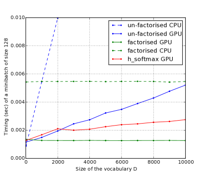
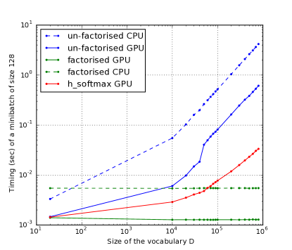
Figure 2: Timing of different algorithms. Time taken by forward and backward propagations in the output layer, including weight update, on a minibatch of size 128 for different sizes of vocabulary D on both CPU and GPU. The input size d is fixed to 300. The Timing of a 2 layer hierarchical softmax efficient GPU implementation (h_softmax) is also provided for comparison. Right plot is in log-log scale. As expected, the timings of factorized versions are independent of the size of the vocabulary.

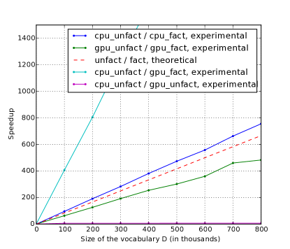
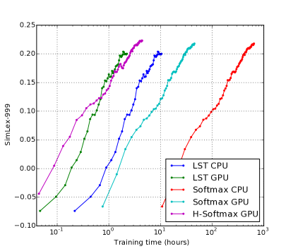
Figure 3: Left: Practical and theoretical speedups for different sizes of vocabulary D and fixed input size d=300. The practical unfact / fact speedup is similar to the theoretical one. Right: Evolution of the Simlex-999 score obtained with different models as a function of training time (CPU softmax times were extrapolated from fewer iterations). Softmax models are zero hidden-layer models, while our large sparse target (LST) models have two hidden layers. These were the best architectures retained in both cases (surprisingly the softmax models with hidden layers performed no better on this task). The extra non-linear layers in LST may help compensate for the lack of a softmax. LST models converge to slightly lower scores at similar speed as the hierarchical softmax model but significantly faster than softmax models.

7 Conclusion and future work

We introduced a new algorithmic approach to efficiently compute the exact gradient updates for training deep networks with very large sparse targets. Remarkably the complexity of the algorithm is independent of the target size, which allows tackling very large problems. Our CPU and GPU implementation yield similar speedups to the theoretical one and can thus be used in practical applications, which could be explored in further work. In particular, neural language models seem good candidates. But it remains unclear how using a loss function other than log-softmax may affect the quality of the resulting word embeddings and further research should be carried out in this direction. While restricted, the spherical family of loss functions, offers opportunities to explore alternatives to the ubiquitous softmax, that thanks to the algorithm presented here, could scale computationally to extremely large output spaces.

References

- Bengio et al. [2001] Yoshua Bengio, Réjean Ducharme, and Pascal Vincent. A neural probabilistic language model. In NIPS’00, pages 932–938. MIT Press, 2001.
- Collobert et al. [2011] R. Collobert, J. Weston, L. Bottou, M. Karlen, K. Kavukcuoglu, and P. Kuksa. Natural language processing (almost) from scratch. Journal of Machine Learning Research, 12:2493–2537, 2011.
- Dauphin et al. [2011] Y. Dauphin, X. Glorot, and Y. Bengio. Large-scale learning of embeddings with reconstruction sampling. In Proceedings of the 28th International Conference on Machine learning, ICML ’11, 2011.
- Jean et al. [2015] Sébastien Jean, Kyunghyun Cho, Roland Memisevic, and Yoshua Bengio. On using very large target vocabulary for neural machine translation. In ACL-IJCNLP’2015, 2015. arXiv:1412.2007.
- Gutmann and Hyvarinen [2010] M. Gutmann and A. Hyvarinen. Noise-contrastive estimation: A new estimation principle for unnormalized statistical models. In Proceedings of The Thirteenth International Conference on Artificial Intelligence and Statistics (AISTATS’10), 2010.
- Mnih and Kavukcuoglu [2013] Andriy Mnih and Koray Kavukcuoglu. Learning word embeddings efficiently with noise-contrastive estimation. In C.J.C. Burges, L. Bottou, M. Welling, Z. Ghahramani, and K.Q. Weinberger, editors, Advances in Neural Information Processing Systems 26, pages 2265–2273. Curran Associates, Inc., 2013.
- Mikolov et al. [2013] T. Mikolov, I. Sutskever, K. Chen, G.S. Corrado, and J. Dean. Distributed representations of words and phrases and their compositionality. In NIPS’2013, pages 3111–3119. 2013.
- Shrivastava and Li [2014] Anshumali Shrivastava and Ping Li. Asymmetric LSH (ALSH) for sublinear time maximum inner product search (MIPS). In Z. Ghahramani, M. Welling, C. Cortes, N.D. Lawrence, and K.Q. Weinberger, editors, Advances in Neural Information Processing Systems 27, pages 2321–2329. Curran Associates, Inc., 2014.
- Vijayanarasimhan et al. [2014] Sudheendra Vijayanarasimhan, Jonathon Shlens, Rajat Monga, and Jay Yagnik. Deep networks with large output spaces. arxiv:1412.7479, 2014.
- Morin and Bengio [2005] Frederic Morin and Yoshua Bengio. Hierarchical probabilistic neural network language model. In Robert G. Cowell and Zoubin Ghahramani, editors, Proceedings of the Tenth International Workshop on Artificial Intelligence and Statistics, pages 246–252. Society for Artificial Intelligence and Statistics, 2005.
- Rumelhart et al. [1986] D.E. Rumelhart, G.E. Hinton, and R.J. Williams. Learning representations by back-propagating errors. Nature, 323:533–536, 1986.
- LeCun [1985] Yann LeCun. Une procédure d’apprentissage pour Réseau à seuil assymétrique. In Cognitiva 85: A la Frontière de l’Intelligence Artificielle, des Sciences de la Connaissance et des Neurosciences, pages 599–604, Paris 1985, 1985. CESTA, Paris.
- LeCun [1986] Yann LeCun. Learning processes in an asymmetric threshold network. In E. Bienenstock, F. Fogelman-Soulié, and G. Weisbuch, editors, Disordered Systems and Biological Organization, pages 233–240. Springer-Verlag, Berlin, Les Houches 1985, 1986.
- Bergstra et al. [2010] James Bergstra, Olivier Breuleux, Frédéric Bastien, Pascal Lamblin, Razvan Pascanu, Guillaume Desjardins, Joseph Turian, David Warde-Farley, and Yoshua Bengio. Theano: a CPU and GPU math expression compiler. In Proceedings of the Python for Scientific Computing Conference (SciPy), 2010. Oral Presentation.
- Bastien et al. [2012] Frédéric Bastien, Pascal Lamblin, Razvan Pascanu, James Bergstra, Ian J. Goodfellow, Arnaud Bergeron, Nicolas Bouchard, and Yoshua Bengio. Theano: new features and speed improvements. Deep Learning and Unsupervised Feature Learning NIPS 2012 Workshop, 2012.
- van Merriënboer et al. [2015] B. van Merriënboer, D. Bahdanau, V. Dumoulin, D. Serdyuk, D. Warde-Farley, J. Chorowski, and Y. Bengio. Blocks and Fuel: Frameworks for deep learning. ArXiv e-prints, jun 2015.