A New Framework for Magnetohydrodynamic Simulations with Anisotropic Pressure

Abstract

We describe a new theoretical and numerical framework of the magnetohydrodynamic simulation incorporated with an anisotropic pressure tensor, which can play an important role in a collisionless plasma. A classical approach to handle the anisotropy is based on the double adiabatic approximation assuming that a pressure tensor is well described only by the components parallel and perpendicular to the local magnetic field. This gyrotropic assumption, however, fails around a magnetically neutral region, where the cyclotron period may get comparable to or even longer than a dynamical time in a system, and causes a singularity in the mathematical expression. In this paper, we demonstrate that this singularity can be completely removed away by the combination of direct use of the 2nd-moment of the Vlasov equation and an ingenious gyrotropization model. Numerical tests also verify that the present model properly reduces to the standard MHD or the double adiabatic formulation in an asymptotic manner under an appropriate limit.

1 Introduction

It is often the case that space and astrophysical phenomena occur in collisionless plasmas, in which the gas is so hot and dilute that the mean free path of charged particles become larger than a scale size of the system. To investigate such complicated collisionless systems, numerical simulations can be powerful tools. In fact, particle-in-cell (PIC) simulations and Vlasov simulations are typical numerical methods to solve the Vlasov-Maxwell system, which is fundamental equations describing time evolution of the velocity distribution function and electromagnetic fields. Although these models can capture all the important kinetic physics self-consistently, because of limited computational resources, it is still hard to apply the methods to phenomena occurring in a scale by far larger than kinetic scales, such as Larmor radii and inertial lengths (but still smaller than mean free paths). The Earth’s magnetosphere [e.g., 18, 9, 28, 4] and the solar wind [e.g., 22, 40, 5] are the typical examples of such large-scale collisionless plasmas in the solar system. As an astrophysical example, a radiatively inefficient accretion flow model of accretion disks is also thought to consist of a collisionless plasma [e.g., 26, 32, 33].

One classical approach to deal with both dynamical scales and kinetic scales is the so-called kinetic magnetohydrodynamics (MHD), which can take into account some of kinetic effects. This philosophy has given rise to the well-known double adiabatic approximation, or Chew-Goldberger-Low (CGL) model [7], which pays special attention to the effect of anisotropy of a distribution function. Since an orbit of a charged particle in a magnetized plasma essentially consists of the gyromotion around a magnetic field line and the parallel motion along the field line, the distribution of kinetic energies contained in the two different motions may differ from each other. Such a situation requires us to extend the standard MHD with a scalar pressure so as to handle an anisotropic pressure tensor. The double adiabatic approximation is a natural extension of the one-temperature MHD, where only the parallel and perpendicular components of a pressure tensor are solved. This is one of the simplest equations of states as a closure for moment hierarchy, assuming that a pressure is completely gyrotropic and the third or higher moments are neglected. The property of this formulation has been studied for decades and has achieved certain degree of success [e.g., 23, 15, 16, 29].

The gyrotropic formulation in the CGL approximation, however, involves a numerical and theoretical difficulty in handling magnetic null points. This arises from the fact that the direction of the magnetic field must be defined for the decomposition of a pressure tensor into parallel and perpendicular components. From the numerical point of view, the determination of the unit vector parallel to the magnetic field, $\hat{\mathbf{b}}=\mathbf{B}/\left|B\right|$, will raise zero-division in a magnetic null point, which severely destroys numerical simulations. When one employs the form of a conservation law, the conservative variable related to the first adiabatic invariant involves the magnetic field in the denominator as well. This drawback may become critical when, for example, considering a current sheet without a guide field, which contains a magnetically neutral line in its own right. The role of pressure anisotropy on collisionless magnetic reconnection, therefore, cannot be studied in the framework of the CGL equations.

This breakdown apparently comes from the strong assumption that a pressure tensor can be well described by the gyrotropic form, or in other words, the gyro-motion is well-defined in a much shorter time scale compared with a concerned dynamical time scale. If a magnetic field is so weak that the gyro period becomes comparable to the dynamical scale, the parallel and perpendicular motion cannot be distinguished from each other and the gyrotropic approximation is no longer valid. As long as we are stuck to the gyrotropic limit, therefore, the problem of zero-division at magnetic null points will not be eliminated completely, regardless of the form of equations of states employed.

With this point in mind, we relax the assumption of the gyrotropic pressure, and extend the equations of states so as to allow finite deviation from gyrotropic formulation. This paper focuses on such a natural extension of MHD following the context of a governing equation describing a more general form of a pressure tensor. Desirable characteristics on the constructed theoretical and numerical framework are, (1) avoidance of numerical difficulty due to zero-division at magnetically neutral region, (2) removal of any temporal and spatial scales related to kinetic physics, (3) convergence to the gyrotropic and isotropic formulation, respectively, under appropriate limits, and (4) an easy modification from an existing MHD code. In this paper, we successfully derive a new framework satisfying the above requirements by evolving a 2nd-rank pressure tensor directly, and develop a corresponding extended MHD code.

The present paper is organized as follows. First, we derive our analytical formulation in section 2. Next, section 3 describe the actual implementation to our simulation code based on the finite difference approach. The numerical behavior is tested in section 4. Finally, section 5 is devoted to summary and concluding remarks.

2 Formulation

2.1 Generalized Energy Conservation Law

In this subsection, we will briefly derive our fluid model starting from the Vlasov equation,

$$\frac{\partial f_{s}}{\partial t}+{\mathbf{v}_{s}}\cdot\nabla f_{s}+\frac{q_{s}}{m_{s}}\left(\mathbf{E}+\frac{\mathbf{v_{s}}}{c}\times\mathbf{B}\right)\cdot\nabla_{\mathbf{v}}f_{s}=0,$$ (1)

where the subscript $s$ indicates the species of charged particles, which are assumed to be ions, $i$, and electrons, $e$, in this paper. The other notations are standard. Taking a second moment of the particle velocity $\mathbf{v}_{s}$ in Eq. (1), we obtain a kinetic stress tensor equation as follows:

$$\frac{\partial}{\partial t}\left(m_{s}n_{s}\mathbf{V}_{s}\mathbf{V}_{s}+\mathbf{P}_{s}\right)+\nabla\cdot\left[m_{s}n_{s}\mathbf{V}_{s}\mathbf{V}_{s}\mathbf{V}_{s}+\left(\mathbf{V}_{s}\mathbf{P}_{s}\right)^{S}+\mathbf{Q}_{s}\right]$$

$$=q_{s}n_{s}\left[\mathbf{V}_{s}\left(\mathbf{E}+\frac{\mathbf{V}_{s}}{c}\times\mathbf{B}\right)\right]^{S}+\frac{q_{s}}{m_{s}c}\left(\mathbf{P}_{s}\times\mathbf{B}\right)^{S},$$ (2)

where the superscript $S$ denotes symmetrization. More specifically, $\left(\mathbf{VP}\right)^{S}_{ijk}=V_{i}P_{jk}+V_{j}P_{ik}+V_{k}P_{ij}$ and $\left(\mathbf{VE}\right)^{S}_{ij}=V_{i}E_{j}+V_{j}E_{i}$, respectively. The moment variables are defined as

$$n_{s} = \int f_{s}d\mathbf{v}_{s},$$ (3)

$$n_{s}\mathbf{V}_{s} = \int\mathbf{v}_{s}f_{s}d\mathbf{v}_{s},$$ (4)

$$\mathbf{P}_{s} = m_{s}\int\left(\mathbf{v}_{s}-\mathbf{V}_{s}\right)\left(\mathbf{v}_{s}-\mathbf{V}_{s}\right)f_{s}d\mathbf{v}_{s},$$ (5)

$$\mathbf{Q}_{s} = m_{s}\int\left(\mathbf{v}_{s}-\mathbf{V}_{s}\right)\left(\mathbf{v}_{s}-\mathbf{V}_{s}\right)\left(\mathbf{v}_{s}-\mathbf{V}_{s}\right)f_{s}d\mathbf{v}_{s}.$$ (6)

Note that the last term in Eq. (2) becomes zero if $\mathbf{P}_{s}$ is exactly gyrotropic. As in derivation of the standard MHD, let us define the one-fluid moments by

$$\rho = \sum_{s}m_{s}n_{s},$$ (7)

$$\rho\mathbf{V} = \sum_{s}m_{s}n_{s}\mathbf{V}_{s},$$ (8)

$$\rho\mathbf{VV}+\mathbf{P} = \sum_{s}\left(m_{s}n_{s}\mathbf{V}_{s}\mathbf{V}_{s}+\mathbf{P}_{s}\right),$$ (9)

$$\rho\mathbf{VVV}+\left(\mathbf{VP}\right)^{S}+\mathbf{Q} = \sum_{s}\left[m_{s}n_{s}\mathbf{V}_{s}\mathbf{V}_{s}\mathbf{V}_{s}+\left(\mathbf{V}_{s}\mathbf{P}_{s}\right)^{S}+\mathbf{Q}_{s}\right].$$ (10)

Then, it is straightforward to show that taking sum of Eq. (2) about the species $s$ leads to

$$\frac{\partial}{\partial t}\left(\rho\mathbf{VV}+\mathbf{P}\right)+\nabla\cdot\left[\rho\mathbf{VVV}+\left(\mathbf{VP}\right)^{S}+\mathbf{Q}\right]$$ (11)

$$=\left[\mathbf{V}\left(\frac{\mathbf{J}}{c}\times\mathbf{B}\right)+\mathbf{J}\left(\mathbf{E}+\frac{\mathbf{V}}{c}\times\mathbf{B}-\frac{\mathbf{J}}{enc}\times\mathbf{B}\right)+\sum_{s}\Omega_{cs}\mathbf{P}_{s}\times\hat{\mathbf{b}}\right]^{S},$$

where $\mathbf{J}=\sum_{s}q_{s}n_{s}\mathbf{V}_{s}$ is the total current density, $\Omega_{cs}=q_{s}B/m_{s}c$ is the cyclotron frequency of the species $s$, and $\hat{\mathbf{b}}=\mathbf{B}/B$ is the unit vector parallel to the magnetic field. In the derivation, we assume the quasi-neutrality, $n\simeq n_{i}\simeq n_{e}$, and neglect the electron inertial effect, i.e., $m_{e}/m_{i}\ll 1$ is used. It is worth noting that the right-hand side of Eq. (11) becomes much simpler by employing the Ohm’s law under the ideal MHD or Hall-MHD ordering. The electric field related to convection, $\mathbf{E}^{\rm conv}=-(\mathbf{V}/c)\times\mathbf{B}$, and to the Hall effect, $\mathbf{E}^{\rm Hall}=(\mathbf{J}/enc)\times\mathbf{B}$, precisely vanish, while the effect of electron pressure remains if Hall-MHD ordering is assumed. Another characteristic is that the trace of the right-hand side reduces to just $\mathbf{J}\cdot\mathbf{E}$, which is consistent with the conservation law of the kinetic and thermal energy in a scalar form.

In addition to the kinetic components, we will derive the semi-conservative form using Faraday’s law, which is a counterpart of the conservation law of total energy in the standard MHD. Throughout this paper, the factor $1/\sqrt{4\pi}$ will be absorbed into the definition of the magnetic field. After some algbra, we obtain the following equation for the $ij$-component,

$$\partial_{t}\left(\rho V_{i}V_{j}+P_{ij}+B_{i}B_{j}\right)$$ (12)

$$+\partial_{k}\left(\rho V_{i}V_{j}V_{k}+P_{ij}V_{k}+P_{ik}V_{j}+P_{jk}V_{i}+Q_{ijk}+\mathcal{S}_{kij}+\mathcal{S}_{kji}\right)$$

$$=J_{i}\left(E_{j}-E_{j}^{\rm conv}-E_{j}^{\rm Hall}\right)+J_{j}\left(E_{i}-E_{i}^{\rm conv}-E_{i}^{\rm Hall}\right)-E_{l}\left(\mathcal{J}_{lij}+\mathcal{J}_{lji}\right)$$

$$+\left(V_{i}\varepsilon_{jkl}J_{k}B_{l}+V_{j}\varepsilon_{ikl}J_{k}B_{l}\right)/c+\sum_{s}\Omega_{cs}\left(\varepsilon_{ikl}P_{s,jk}\hat{b}_{l}+\varepsilon_{ikl}P_{s,ik}\hat{b}_{l}\right),$$

where $\varepsilon_{ijk}$ denotes the Levi-Civita symbol, and Einstein’s summation convention is applied to repeated indices. The newly introduced notations, $\mathcal{S}_{kij}$ and $\mathcal{J}_{kij}$, are defined as

$$\mathcal{S}_{kij} = c\varepsilon_{kli}E_{l}B_{j},$$ (13)

$$\mathcal{J}_{kij} = c\varepsilon_{kli}\partial_{l}B_{j},$$ (14)

which reduce to the Poynting flux and the current density, respectively, if one takes their trace with respect to $i$ and $j$.

Eq. (12) is a general result, which is valid for a large mass ratio, or in other words, a scale size of the system is much larger than the electron skin depth. In a particular case where the ideal MHD ordering can be applied reasonably, that is, where all the temporal and the spatial scales are much larger than the cyclotron period and the inertial length of ions, respectively, we can employ the simplest Ohm’s law,

$$\mathbf{E}+\frac{\mathbf{V}}{c}\times\mathbf{B}=0,$$ (15)

and the right-hand side of Eq. (12), except for the last two terms related to cyclotron frequencies, is then simplified as

$$V_{k}\partial_{k}\left(B_{i}B_{j}\right)-V_{i}\partial_{j}\left(\frac{B^{2}}{2}\right)-V_{j}\partial_{i}\left(\frac{B^{2}}{2}\right).$$ (16)

Again, Eq. (16) reduces to zero by taking the trace. Inclusion of other physics such as finite resistivity and the Hall effect is straightforward by direct use of Eq. (12) and appropriate modification of the Ohm’s law.

In this paper, for simplicity we will neglect the generalized heat flux tensor, $\mathbf{Q}$. Generally speaking, it is very common that a collisionless plasma does not reach its local thermodynamical equilibrium, and the deviation from the Maxwellian distribution plays a crucial role in dynamical phenomena in a collisionless system. Nevertheless, since the purpose of this paper is to develop a method to treat an anisotropic pressure, we do not take in account the heat flux tensor $\mathbf{Q}$. If one intends to include the effect of the heat flux, $\mathbf{Q}$ should be determined by using an appropriate closure model [e.g., 19, 39].

2.2 Gyrotropization Model

The last two terms in Eq. (12) contain the cyclotron frequencies, $\Omega_{cs}$, which cannot be resolved under the MHD ordering. Therefore, these terms may be replaced by an effective collision model. [13] describes a gyrotropization model of an anisotropic pressure tensor, which assumes that a pressure tensor approaches to a gyrotropic one, $\mathbf{P}_{g}=P_{\perp}\mathbf{I}+\left(P_{||}-P_{\perp}\right)\hat{\mathbf{b}}\hat{\mathbf{b}}$, with a certain relaxation time scale. The functional form of the collision operator used in this work is as follows,

$$\left[\frac{\partial\mathbf{P}}{\partial t}\right]_{\rm collision}=-\nu_{g}\left(\mathbf{P}-\mathbf{P}_{g}\right).$$ (17)

The effective collision frequency, $\nu_{g}=\nu_{g}\left(B\right)$, is a function of the local magnetic field strength, and must be much higher than the highest frequency of the system. While [13] adopts a constant $\nu_{g}$ both in space and time, we assume that it is proportional to the local magnetic field strength because the original time scale is determined by the cyclotron period. The dependence on the magnetic field is consistent with the physical insight that finite non-gyrotropy will remain at an unmagnetized region due to lack of any cyclotron motion.

The employment of the effective collision model successfully eliminates any scales related to the cyclotron motion, and we can solve the set of all basic equations in the framework of only fluid-based variables. Moreover, it is remarkable that, by introducing the nongyrotropic pressure tensor and the gyrotropization model described here, any numerical difficulty in dealing with magnetically neutral regions is completely removed. Although we still need to determine the direction of the local magnetic field for calculation of an asymptote in the collision model, the gyrotropic pressure will never be used at magnetic null points because $\nu_{g}$ vanishes there by the assumption of $\nu_{g}\propto B$.

Finally, all the governing equations employed throughout this paper are summarized here. We solve the set of (generalized) conservation laws for the mass, momentum and total energy, and the induction equation under the ordering of the ideal MHD,

$$\frac{\partial\rho}{\partial t}+\nabla\cdot\left(\rho\mathbf{V}\right)=0,$$ (18)

$$\frac{\partial\left(\rho\mathbf{V}\right)}{\partial t}+\nabla\cdot\left(\rho\mathbf{VV}+\mathbf{P}+\frac{B^{2}}{2}\mathbf{I}-\mathbf{BB}\right)=0,$$ (19)

$$\frac{\partial\mathbf{B}}{\partial t}=\nabla\times\left(\mathbf{V}\times\mathbf{B}\right),$$ (20)

$$\frac{\partial}{\partial t}\left(\rho V_{i}V_{j}+P_{ij}+B_{i}B_{j}\right)$$ (21)

$$+\partial_{k}\left[\rho V_{i}V_{j}V_{k}+P_{ij}V_{k}+P_{ik}V_{j}+P_{jk}V_{i}+\mathcal{S}_{kij}+\mathcal{S}_{kji}\right]$$

$$=B_{i}V_{k}\partial_{k}B_{j}+B_{j}V_{k}\partial_{k}B_{i}-B_{k}V_{i}\partial_{j}B_{k}-B_{k}V_{j}\partial_{i}B_{k}-\nu_{g}\left(P_{ij}-P_{g,ij}\right).$$

Since the pressure tensor is symmetric by definition, we have 13 independent variables in total; $\rho,V_{x},V_{y},V_{z},B_{x},B_{y},B_{z},P_{xx},P_{yy},P_{zz},P_{xy},P_{yz},P_{zx}$.

3 Numerical Implementation

In this section, our implementation of the present model is described. Existing MHD codes written in the conservative forms can be readily extended to the present model with slight modification, since we can derive the basic equations in the form of semi-conservation laws accompanied by several directional energy exchange terms and a collision term. We describe here the spatially and temporally 2nd-order finite difference algorithms, and elucidate differences from standard MHD codes. Unless otherwise noted, test problems described in the next section employ this 2nd-order implementation. Of course, other methods such as finite volume approaches can be used as well.

In the following, for simplicity let us consider a one-dimensional case, and write Eqs. (18) through (21) together as

$$\frac{\partial\mathbf{U}}{\partial t}+\frac{\partial\mathbf{F}}{\partial x}+\mathbf{A}\frac{\partial\mathbf{U}}{\partial x}=-\nu_{g}\left(\mathbf{U}-\mathbf{U}_{g}\right),$$ (22)

where $\mathbf{U}=\left\{\rho,\ \rho\mathbf{V},\ \mathbf{B},\ \rho\mathbf{VV}+\mathbf{P}+\mathbf{BB}\right\}\in\mathbb{R}^{13}$ contains conservative variables, and $\mathbf{A}\in\mathbb{R}^{13}\times\mathbb{R}^{13}$ describes the energy exchange terms. Note that $\mathbf{A}$ has non-zero elements only for Eq. (21) and each element always consists of the products of the velocity and the magnetic field, $V_{\alpha}B_{\beta}$.

Extension to a multi-dimensional problem is straightforward as far as our newly introduced parts are concerned, while the issue on numerical divergence error of magnetic field must be resolved as in the case of the standard MHD. In our code, the constrained transport (CT) treatment [10, 38] is adopted to avoid this problem. In particular, we utilized the Harten-Lax-van Leer (HLL) upwind-CT method [31, 1], in which electric fields are interpolated to edge centers using the same interpolation scheme as used for other fluid variables and the HLL approximate Riemann solver [14]. One may employ any other divergence cleaning techniques, since the present model does not alter the property of the induction equation.

3.1 Conservative Part

We solve Eq. (22) by means of operator splitting into three parts, i.e., a conservative term $\partial\mathbf{F}/\partial x$, a non-conservative term $\mathbf{A}\partial\mathbf{U}/\partial x$, and an effective collision term $-\nu_{g}\left(\mathbf{U}-\mathbf{U}_{g}\right)$. In this subsection, we first review the integration method for the conservative part.

Let us consider an equally spaced one-dimensional computational domain where the range of $j$-th cell is denoted as $x\in\left[x_{j}-\Delta x/2,x_{j}+\Delta x/2\right]$ with the mesh size $\Delta x$. All the primitive variables $\mathbf{W}=\left\{\rho,\ \mathbf{V},\ \mathbf{B},\ \mathbf{P}\right\}$ are defined at each cell center, $x_{j}$, as point values. Then, $\mathbf{W}_{j}$ is linearly interpolated to the face center, $x_{j\pm 1/2}$, with an appropriate limiter function,

$$\mathbf{W}_{L,j+1/2}=\mathbf{W}_{j}+\frac{1}{2}{\rm minmod}\left(\mathbf{W}_{j+1}-\mathbf{W}_{j},\mathbf{W}_{j}-\mathbf{W}_{j-1}\right),$$ (23)

$$\mathbf{W}_{R,j-1/2}=\mathbf{W}_{j}-\frac{1}{2}{\rm minmod}\left(\mathbf{W}_{j+1}-\mathbf{W}_{j},\mathbf{W}_{j}-\mathbf{W}_{j-1}\right),$$ (24)

where we employ the minmod limiter to suppress numerical oscillation around discontinuities. Once the left and right states across the cell faces $\{\mathbf{W}_{L,R}\}$ are interpolated, we can immediately obtain the corresponding conservative variables and fluxes, $\{\mathbf{U}_{L,R}\}$ and $\{\mathbf{F}_{L,R}\}$, respectively.

Next, we consider a self-similarly expanding Riemann fan at the cell faces. The outermost signal speeds in the present system can be evaluated by the largest and smallest eigenvalues of the matrix $\left(\partial\mathbf{F}/\partial\mathbf{U}\right)+\mathbf{A}$, where $\partial\mathbf{F}/\partial\mathbf{U}$ is a Jacobian matrix, as follows:

$$\lambda^{\pm}\left(\mathbf{U}\right) = V_{x}\pm\sqrt{b+\sqrt{b^{2}-c}},$$ (25)

$$b = \frac{1}{2\rho}\left(4P_{xx}+B^{2}\right),$$

$$c = \frac{1}{\rho^{2}}\left[\left(3P_{xx}+B_{y}^{2}+B_{z}^{2}\right)\left(P_{xx}+B_{x}^{2}\right)\right.$$

$$+\left(2P_{xy}-B_{x}B_{y}\right)B_{x}B_{y}$$

$$\left.+\left(2P_{xz}-B_{x}B_{z}\right)B_{x}B_{z}\right].$$

These are the counterparts of fast-magnetosonic waves in the standard MHD. Hereafter, we define the leftward and rightward expansion speeds of the Riemann fan in the form of absolute values,

$$s_{L} = \left|{\rm min}\left\{0,\lambda^{-}\left(\mathbf{U}_{L}\right),\lambda^{-}\left(\mathbf{U}_{R}\right)\right\}\right|,$$ (26)

$$s_{R} = \left|{\rm max}\left\{0,\lambda^{+}\left(\mathbf{U}_{L}\right),\lambda^{+}\left(\mathbf{U}_{R}\right)\right\}\right|.$$ (27)

As in the usual implementation, $s_{L}$ and $s_{R}$ are chosen to reduce to zero in supersonic cases.

Denoting the intermediate state inside the Riemann fan as $\mathbf{U}_{*}$, the conservative and non-conservative parts in Eq. (22) can be integrated over a control volume $\left(x,t\right)\in\left[-Ts_{L},Ts_{R}\right]\times\left[0,T\right]$ and reads

$$\mathbf{U}_{*}\left(s_{R}+s_{L}\right)-\left(\mathbf{U}_{R}s_{R}+\mathbf{U}_{L}s_{L}\right)+\left(\mathbf{F}_{R}-\mathbf{F}_{L}\right)+\int_{\mathbf{U}_{L}}^{\mathbf{U}_{R}}\mathbf{A}\left(\mathbf{U}\right)d\mathbf{U}=0,$$ (28)

where the last term in the left-hand side requires an integral along a phase-space path from a left state through a right state. Following the path-conservative HLL scheme proposed in [8], we evaluate this integral by assuming two piecewise linear paths from $\mathbf{U}_{L}$ to $\mathbf{U}_{*}$, and from $\mathbf{U}_{*}$ to $\mathbf{U}_{R}$, respectively. This linear segment assumption immediately leads to an implicit equation for $\mathbf{U}_{*}$,

$$\mathbf{U}_{*}\left(s_{R}+s_{L}\right)-\left(\mathbf{U}_{R}s_{R}+\mathbf{U}_{L}s_{L}\right)+\left(\mathbf{F}_{R}-\mathbf{F}_{L}\right)$$ (29)

$$+\mathbf{\tilde{A}}\left(\mathbf{U}_{L},\mathbf{U}_{*}\right)\left(\mathbf{U}_{*}-\mathbf{U}_{L}\right)+\mathbf{\tilde{A}}\left(\mathbf{U}_{*},\mathbf{U}_{R}\right)\left(\mathbf{U}_{R}-\mathbf{U}_{*}\right)=0,$$

with

$$\mathbf{\tilde{A}}\left(\mathbf{U}_{a},\mathbf{U}_{b}\right)=\int_{0}^{1}\mathbf{A}\left(\mathbf{U}_{a}+\left(\mathbf{U}_{b}-\mathbf{U}_{a}\right)s\right)ds.$$ (30)

In our implementation, the integral over $s$ is calculated by means of a three-point Gaussian quadrature. Eq. (29) must in general be solved for $\mathbf{U}_{*}$ in an iterative manner. In the present system, however, we do not need iteration practically, since $\tilde{\mathbf{A}}\left(\mathbf{U}_{a},\mathbf{U}_{b}\right)\left(\mathbf{U}_{b}-\mathbf{U}_{a}\right)$ can be evaluated only by $\rho_{*}$, $\left(\rho\mathbf{V}\right)_{*}$ and $\mathbf{B}_{*}$, which are obtained explicitly from Eq. (29). For more detail on path-conservative HLL scheme, see [8].

Using the intermediate state obtained above, we can calculate the path-conservative HLL fluctuations, which explains the modification of the flux from the original point-value flux, as follows:

$$\mathbf{D}_{L}=\frac{s_{L}}{s_{R}+s_{L}}\left[\mathbf{F}_{R}-\mathbf{F}_{L}-s_{R}\left(\mathbf{U}_{R}-\mathbf{U}_{L}\right)+\mathbf{D}_{A}\right],$$ (31)

$$\mathbf{D}_{R}=\frac{s_{R}}{s_{R}+s_{L}}\left[\mathbf{F}_{R}-\mathbf{F}_{L}+s_{L}\left(\mathbf{U}_{R}-\mathbf{U}_{L}\right)+\mathbf{D}_{A}\right],$$ (32)

where the contribution from the non-conservative term is

$$\mathbf{D}_{A}=\mathbf{\tilde{A}}\left(\mathbf{U}_{L},\mathbf{U}_{*}\right)\left(\mathbf{U}_{*}-\mathbf{U}_{L}\right)+\mathbf{\tilde{A}}\left(\mathbf{U}_{*},\mathbf{U}_{R}\right)\left(\mathbf{U}_{R}-\mathbf{U}_{*}\right).$$ (33)

Finally, the conservative part in Eq. (22) can be discretized as

$$\frac{\partial\mathbf{U}_{j}}{\partial t}+\frac{1}{\Delta x}\left(\mathbf{F}_{L,j+1/2}-\mathbf{F}_{R,j-1/2}\right)+\frac{1}{\Delta x}\left(\mathbf{D}_{L,j+1/2}+\mathbf{D}_{R,j-1/2}\right)=0.$$ (34)

In particular, if the non-conservative terms do not exist, or if $\mathbf{D}_{A}=0$, this scheme simply reduces to the usual HLL scheme with $\mathbf{F}_{\rm HLL}=\mathbf{F}_{L}+\mathbf{D}_{L}=\mathbf{F}_{R}-\mathbf{D}_{R}$.

3.2 Energy Exchange Part

When we considered an intermediate state inside an expanding Riemann fan in the previous subsection, the effect of non-conservative terms, $\mathbf{A}\left(\partial\mathbf{U}/\partial x\right)$, was also taken into account to keep the consistency of the present hyperbolic system. It is, however, just for determination of the conservative flux, and the time integration of the non-conservative terms must be carried out separately.

This evaluation requires the magnetic field derivatives. For the purpose of avoiding spurious oscillation near discontinities, one may need to carry out this evaluation with an appropriate limiter function. Our implementation simply adopts the minmod limiter, and spatially discretized as

$$\frac{\partial\mathbf{U}_{j}}{\partial t}+\mathbf{A}_{j}\frac{1}{\Delta x}{\rm minmod}\left(\mathbf{U}_{j+1}-\mathbf{U}_{j},\mathbf{U}_{j}-\mathbf{U}_{j-1}\right)=0.$$ (35)

Then, it is straightforward to temporally integrate Eqs. (34) and (35) together by means of the 2nd-order TVD Runge-Kutta method [35],

$$\mathbf{U}^{*} = \mathbf{U}^{n}-\Delta t\mathcal{L}\left(\mathbf{U}^{n}\right),$$ (36)

$$\mathbf{U}^{n+1} = \frac{1}{2}\mathbf{U}^{n}+\frac{1}{2}\left[\mathbf{U}^{*}-\Delta t\mathcal{L}\left(\mathbf{U}^{*}\right)\right],$$ (37)

where

$$\mathcal{L}\left(\mathbf{U}\right)=\frac{\partial\mathbf{F}\left(\mathbf{U}\right)}{\partial x}+\mathbf{A}\left(\mathbf{U}\right)\frac{\partial\mathbf{U}}{\partial x}.$$ (38)

and (35). The time interval, $\Delta t$, is determined to satisfy the CFL condition for the fastest propagating waves,

$$\Delta t\leq\nu\frac{\Delta x}{{\rm max}_{j}\left\{\left|\lambda^{+}\left(\mathbf{U}_{j}\right)\right|,\left|\lambda^{-}\left(\mathbf{U}_{j}\right)\right|\right\}}$$ (39)

where $\nu$ is a safety parameter fixed to be 0.4 in this paper.

3.3 Effective Collision Part

After calculating the pressure tensor from the updated conservative variables, the effective collision model (17) is applied in every time step and at every grid point. The procedure starts from the determination of the direction of the magnetic field, $\hat{\mathbf{b}}=\mathbf{B}/B$, at each site. Note that, as mentioned in the previous section, we do not require $\hat{\mathbf{b}}$ at an unmagnetized region since there the effective collision frequency in our model becomes precisely zero, and therefore no singularity of division by zero exists.

Our actual implementation is as follows. The pressure tensor defined in $xyz$-space is rotated to the coordinate system aligned with the local magnetic field, so that the index 1 represents the direction parallel to $\hat{\mathbf{b}}$, and the indices 2 and 3 correspond to two different perpendicular directions. Then, the gyrotropic asympote, $\mathbf{P}_{g}$, can be defined as

$$\mathbf{P}_{g}=P_{\perp}\mathbf{I}+\left(P_{||}-P_{\perp}\right)\hat{\mathbf{b}}\hat{\mathbf{b}},$$ (40)

with

$$P_{||}=P_{11},\ \ \ P_{\perp}=\frac{P_{22}+P_{33}}{2}.$$ (41)

Alternatively, when one does not need other components than the parallel and perpendicular ones, simpler expressions

$$P_{||}=\hat{\mathbf{b}}\cdot\mathbf{P}\cdot\hat{\mathbf{b}},\ \ \ P_{\perp}=\frac{{\rm Tr}\mathbf{P}-P_{||}}{2},$$ (42)

can also be used. It is worth noting that by enforcing the isotropy, $P_{||}=P_{\perp}={\rm Tr}\mathbf{P}/3$, the model will reduce to the standard MHD limit.

Once the gyrotropic asymptote is determined, we use the exact solution to Eq. (17) in order to avoid explicit integration of a stiff equation,

$$\mathbf{P}\left(t+\Delta t\right)=\mathbf{P}_{g}+\left(\mathbf{P}\left(t\right)-\mathbf{P}_{g}\right)e^{-\nu_{g}\Delta t},$$ (43)

which is applied on every sub-cycle of the Runge-Kutta time integration.

3.4 Summary of Numerical Method

We have separately discussed the integration method of each term following the spirit of an operator splitting technique. It would be useful to summarize our implementation here. A procedure in one Runge-Kutta subcycle is as follows:

1. Convert all the conservative variables defined at cell centers $\left\{\mathbf{U}\right\}$ to the primitive variables $\left\{\mathbf{W}\right\}$.

2. Interpolate $\left\{\mathbf{W}\right\}$ to cell faces by Eqs. (23) and (24).

3. Calculate the corresponding conservative variables $\left\{\mathbf{U}_{L,R}\right\}$, fluxes $\left\{\mathbf{F}_{L,R}\right\}$, and expansion speeds $\left\{s_{L,R}\right\}$.

4. Solve Eq. (29) for an intermediate state $\left\{\mathbf{U}_{*}\right\}$.

5. Obtain HLL fluctuations $\left\{\mathbf{D}_{L,R}\right\}$ by Eqs. (31) and (32).

6. Define the matrix $\left\{\mathbf{A}_{j}\right\}$ required for evaluation of the non-conservative term.

7. Integrate Eqs. (34) and (35) simultaneously by

   $$\mathbf{U}^{r+1}=\mathbf{U}^{r} - \frac{\Delta t}{\Delta x}\left(\mathbf{F}_{L,j+1/2}-\mathbf{F}_{R,j-1/2}\right)$$ (44)

   $$- \frac{\Delta t}{\Delta x}\left(\mathbf{D}_{L,j+1/2}+\mathbf{D}_{R,j-1/2}\right)$$

   $$- \mathbf{A}_{j}\frac{\Delta t}{\Delta x}{\rm minmod}\left(\mathbf{U}_{j+1}-\mathbf{U}_{j},\mathbf{U}_{j}-\mathbf{U}_{j-1}\right)$$

   where $r$ represents an index of the substep in the Runge-Kutta method.

8. Define parallel and perpendicular pressures, $P_{||,\perp}$, by using Eq. (40) or (41).

9. Gyrotropize the pressure tensor with the solution (43) depending on the local magnetic field strength.

10. Isotropize the pressure tensor if necessary.

11. Set boundary conditions.

This subcycle is repeated twice in each 2nd-order Runge-Kutta cycle. The procedure described here can be easily extended to multi-dimensional problems in a dimension by dimension fashion, since our implementation is based on the finite difference approach.

Note that the fluxes and the fluctuations here are defined as point values. Since the present implementation has only second order of accuracy in space, a point value flux and a numerical flux are identical with each other. When one desires to use a higher than second order accuracy scheme, however, an appropriate conversion formula from a point value to a numerical flux must be applied [35]. In A, we describe an example of higher-order implementation using the 5th-order weighted essentially non-oscillatory (WENO) scheme [27] and 3rd-order TVD Runge-Kutta scheme [35].

4 Test Problems

This section shows a series of test problems, including one-, two- and three-dimensional application. As well as non-gyrotropic cases, we will put a certain degree of emphasis on gyrotropic and isotropic limits, which can be compared with published results.

4.1 Shock Tube Problem

4.1.1 Fast Isotropization

First, results of the shock tube problem described in [3] are shown in this subsection, which is one of the most widely used test problems for the MHD system to check, particularly, the accuracy and the resolution for propagating waves including discontinuities such as shock waves and contact discontinuities.

A one-dimensional simulation domain with $x\in\left[-1,1\right]$ is discretized by equally spaced 1000 grid points. The initial state is originally given as

$$\left(\rho,V_{x},V_{y},V_{z},B_{y},B_{z},P\right)=\left\{\begin{array}[]{ll}\left(1.0,0.0,0.0,0.0,1.0,0.0,1.0\right)&(x\leq 0),\\ \left(0.125,0.0,0.0,0.0,-1.0,0.0,0.1\right)&(x>0).\end{array}\right.$$ (47)

The normal component of the magnetic field is constant in time and space from the constraint of $\nabla\cdot{\mathbf{B}}=0$, and is set to be $B_{x}=0.75$. Since now we have to give the gas pressure in a tensor form, let us assume that the initial plasma has an isotropic distribution in velocity space, that is, $\mathbf{P}=P\mathbf{I}$ is assumed at $t=0$. Then we integrate the governing equations (18) through (21) until $t=0.2$.

Fig. 1 shows the results under an isotropic limit. Namely, in addition to the gyrotropization, fast isotropization is also assumed by enforcing $P_{||}=P_{\perp}$ in Eq. (40) as described in Sec. 3.3. The solid line overplotted in each panel represents the reference solution calculated by Athena code with 20000 grid points [37]. We can see that the solution under the isotropic limit properly converges to the standard MHD result. A couple of fast rarefaction waves propagate away toward both directions at first, behind which a slow shock and a slow-mode compound wave make the steep structure. Between these slow-mode related waves, a contact discontinuity is formed, where only the density profile has a discontinuous jump. It should be noted that the effective adiabatic index in this case is $\gamma=5/3$ rather than $\gamma=2$ as in the original problem setting. Nevertheless, the basic structure is still quite similar to each other except for slight modification of the wave propagation speeds.

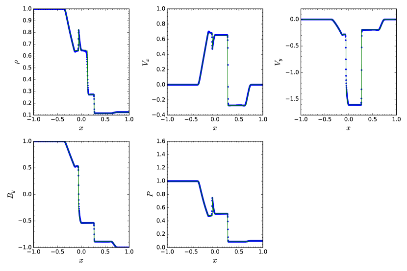
Figure 1: Brio-Wu shock tube problem under an isotropic MHD limit. The data is taken at $t=0.2$. The solid line overplotted in each panel is the reference solution calculated by using Athena code with 20000 grid points. In the reference run, Roe approximate Riemann solver, piecewise constant interpolation, and corner transport upwind integrator are employed.

4.1.2 Fast Gyrotropization

Next, we consider the case under the gyrotropic limit. Although the present formulation exactly preserves the total energy, the amount of heating due to numerical viscosity and resistivity distributed to each pressure component cannot be determined self-consistently. This fact results in the absence of exact Rankine-Hugoniot jump conditions, and the dependency of solutions on numerical schemes employed in a specific code. One possible prescription to avoid this undesired dependency is inclusion of viscosity and/or resistivity models which describe the heating rate in each direction. The simplest assumption on resistivity is, for example, the isotropic heating, i.e., one-third of Joule heating is equally deposited in $P_{xx}$, $P_{yy}$, and $P_{zz}$, respectively, based on the physical consideration that the resistive heating is mainly carried by electrons, which may isotropize much faster than a dynamical time scale. Nevertheless, we particularly focus on the ideal Ohm’s law in this paper to demonstrate the capability of our model to track dynamical development.

The results under the gyrotropic limit are plotted in Fig. 2 with the same format as in Fig. 1. Note that, since the simulation domain contains a finite magnetic field everywhere and we assume a very large gyrotropization rate, the governing equations asymptotically reduce to the double adiabatic approximation, or CGL limit. There is, unfortunately, no reference solution to which we can reasonably compare our nearly double adiabatic results, so here we only mention remarkable differences from the isotropic case.

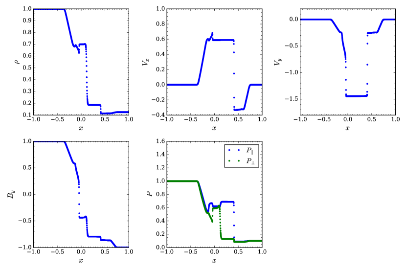
Figure 2: Brio-Wu shock tube problem under a gyrotropic MHD limit. The data is taken at $t=0.2$.

One noteworthy change is that the contact discontinuity around $x\sim 0.2$ involves variation not only in $\rho$ but also in $B_{y}$, $P_{||}$, and $P_{\perp}$. This modified jump condition can be understood from the momentum conservation law across a boundary without mass flux,

$$\left[P_{\perp}+\frac{B^{2}}{2}-\left(1-\frac{P_{||}-P_{\perp}}{B^{2}}\right)B_{x}^{2}\right]_{1}^{2}=0,$$ (48)

$$\left[-\left(1-\frac{P_{||}-P_{\perp}}{B^{2}}\right)B_{x}B_{y}\right]_{1}^{2}=0,$$ (49)

where $\left[X\right]_{1}^{2}=X_{2}-X_{1}$ indicates a difference between two separated regions. These relations imply that the total pressure, $P_{\perp}+B^{2}/2$, and the tangential magnetic field, $B_{y}$, may change across the boundary if the pressure anisotropy also changes while satisfying the conservation laws. In terms of linear waves, a newly introduced degree of freedom related to the pressure anisotropy produces a different kind of entropy waves, whose eigenfunction can have perturbations in the pressure and the magnetic field.

Another notable feature is the selective enhancement of the parallel pressure across the slow shock. This firehose-type anisotropy is consistent with a direct consequence from conservation of the first and second adiabatic invariants. The combination of the first and second adiabatic invariants, $P_{\perp}/\left(\rho B\right)={\rm const.}$ and $B^{2}P_{||}/\rho^{3}={\rm const.}$, tells us that, along motion of a fluid element, increasing density and decreasing magnetic field strength lead to large enhancement of parallel pressure. From the first adiabatic invariant, on the other hand, perpendicular pressure is proportional to a product of density and magnetic field strength, which results in a smaller increase in the perpendicular pressure across the slow shock.

4.1.3 Without Gyrotropization

Our implementation works well even when gyrotropization is completely turned off. Since this limit implies an infinitely large gyro radius of ions, it should be appropriate to adopt more sophisticated Ohm’s law, for example, with the Hall term. Although we provide only the results with the ideal Ohm’s law here for theoretical simplicity, a more general electric field can be employed in a straightforward manner by going back to Eq. (12) instead of Eq. (21).

Roughly speaking, the qualitative behavior discussed above does not largely change even in the case without gyrotropiazation. The profiles of variables in this case are shown in Fig. 3. The wave structure, again, consists of a pair of fast rarefaction waves, slow-mode shock and compound waves, and a contact discontinuity accompanied by variations in the tangential magnetic field and the pressure anisotropy. It should be noted that, in one-dimensional problems, $P_{yy}$ and $P_{zz}$ only act as passive variables described by the following equation,

$$\frac{\partial P_{ii}}{\partial t}+\frac{\partial}{\partial x}\left(V_{x}P_{ii}\right)+2P_{ix}\frac{\partial V_{i}}{\partial x}=0,$$ (50)

where $i=y,z$, so the relatively large jump of $P_{yy}$ across the contact discontinuity, for instance, can have no back reaction to the plasma flow. In particular, the coplanarity in the present setup, i.e., $V_{z}=0$ and $B_{z}=0$, reduces the energy equation about a $zz$-component to a simple continuity equation for $P_{zz}$, which makes the behavior of $P_{zz}$ quantitatively same as of $\rho$.

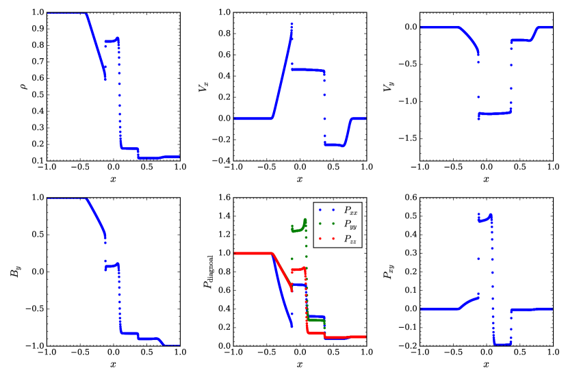
Figure 3: Brio-Wu shock tube problem with no gyrotropization effect. The data is taken at $t=0.2$.

4.2 One-dimensional Reconnection Layer

This subsection provides another set of the one-dimensional Riemann problem described in [21] (hereafter HH13), who discusses the wave structure in a self-similarly developing reconnection layer by paying attention to the properties of a slow-mode wave and an Alfvén wave under the double adiabatic approximation, i.e., the gyrotropic limit. In contrast to a coplanar case discussed in the previous subsection, we particularly focus on a non-coplanar problem, where the degeneracy of a shear Alfvén wave and other modes may be removed.

The initial condition is an isotropic and isothermal Harris-type current sheet with a uniform guide field,

$$B_{y}\left(x\right) = B_{0}\ \cos\phi\ \tanh\left(x/L\right),$$ (51)

$$B_{z}\left(x\right) = B_{0}\ \sin\phi,$$ (52)

where $B_{0}$ is the magnetic field strength at the lobe region, $\phi$ is the angle between the lobe magnetic field and $x$-axis, and $L$ is the half width of the current sheet. The initially isotropic pressure balance is determined so as to set the plasma beta, $\beta=2P/B^{2}$, measured at the lobe region to 0.25. Once the normal magnetic field, $B_{x}$, is superposed, fast rarefaction waves, rotational discontinuities, and slow shocks propagate away from the current sheet toward both lobes. Here the magnitude of $B_{x}$ is chosen to be 5% of $B_{0}$. The simulation domain, $-200L\leq x\leq 200L$, is discretized by 2000 grid points, and the free boundary conditions are assumed at $|x|=200L$. For normalization, we set $L$, $B_{0}$ and the lobe density, $\rho_{0}$, to be unity, which implies that the velocity and the pressure are normalized by $V_{A}=B_{0}/\sqrt{\rho_{0}}$ and $B_{0}^{2}$, respectively.

4.2.1 Fast Isotropization

First, Fig. 4 shows the snapshots in the case with fast isotropization at time $t=3500$, before which a pair of fast rarefaction waves propagated away from the simulation domain. The angle $\phi$ is set to be $30^{\circ}$. Note that this run is comparable to left panels of Fig. 1 in HH13. From the panel showing the profiles of the magnetic field, we can see that a pair of rotational discontinuities around $\left|x\right|\sim 110$ rotate all the magnetic field to $z$-direction. Then slow shocks at $\left|x\right|\sim 75$, which we can observe in all panels, dissipate the field energy contained in $B_{z}$. This behavior is common to the standard MHD independently of the initial angle $\phi$, and our model properly retains qualitatively the same structure as in the isotropic MHD even with the propagation of shearing Alfvén waves included.

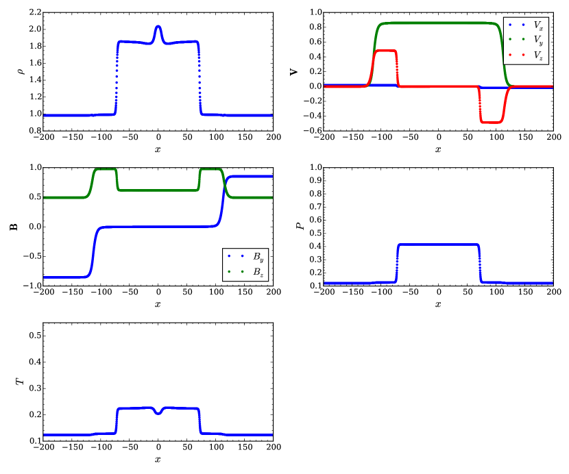
Figure 4: The results of a one-dimensional Riemann problem to imitate a self-similar reconnection layer, assuming fast isotropization. The data is taken at $t=3500$

4.2.2 Fast Gyrotropization

Fig. 5, on the other hand, shows the same plots except that only gyrotropization is assumed. Since the uniform and constant normal magnetic field is imposed in this one-dimensional problem, each grid point always has a finite magnetic field strength, which leads this calculation to the almost same one in the double adiabatic limit. Fig. 5 is, therefore, now comparable to right panels of Fig. 1 in HH13, and again all the profiles well agree with each other in a quantitative manner. In particular, the reversal of propagation speeds of slow-mode waves ($\left|x\right|\sim 150$) and Alfvén waves ($\left|x\right|\sim 90$), weakness of the slow shocks in terms of the released magnetic energy, and the parallel pressure enhancement across the slow shocks, are correctly captured. As already mentioned in the previous subsection, in addition, the contact discontinuity remaining around $x\sim 0$ can sustain variations in the magnetic field and the pressure anisotropy in contrast to the flat profiles in Fig. 4.

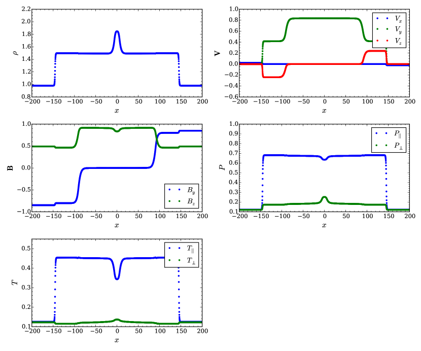
Figure 5: The results of a one-dimensional Riemann problem to imitate a self-similar reconnection layer, assuming fast gyrotropization. The data is taken at $t=3500$.

4.2.3 Without Gyrotropization

It is remarkable that, if any gyrotropization and isotropization effects are neglected, the present model shows no evidence of magnetic reconnection, as demonstrated in Fig. 6. The final state in this case is simply a dynamical equilibrium sustained by a contact discontinuity satisfying

$$\left[\rho V_{x}^{2}+P_{xx}+\frac{B^{2}}{2}\right]^{1}_{2}=0,$$ (53)

$$\left[\rho V_{x}V_{y}+P_{xy}-B_{x}B_{y}\right]^{1}_{2}=0,$$ (54)

$$\left[\rho V_{x}V_{z}+P_{zx}-B_{x}B_{z}\right]^{1}_{2}=0,$$ (55)

where the leftmost term in each equation vanishes since $V_{x}$ is zero across the contact discontinuity. Focusing on $y$-direction, for example, the initial state is in dynamical imbalance by the magnetic tension force, $-B_{x}B_{y}$, due to the existence of additionally imposed $B_{x}$. Since the present assumption adds five extra degrees of freedom, this system has six independent entropy modes in total, i.e.,

$$\left(\delta\rho,\ \delta\mathbf{V},\ \delta B_{y},\ \delta B_{z},\ \delta P_{xx},\ \delta P_{yy},\ \delta P_{zz},\ \delta P_{xy},\ \delta P_{yz},\ \delta P_{zx}\right)$$

$$=\left\{\begin{array}[]{l}(1,\ \mathbf{0},\ 0,\ 0,\ 0,\ 0,\ 0,\ 0,\ 0,\ 0),\\ (0,\ \mathbf{0},\ 0,\ 0,\ 0,\ 1,\ 0,\ 0,\ 0,\ 0),\\ (0,\ \mathbf{0},\ 0,\ 0,\ 0,\ 0,\ 1,\ 0,\ 0,\ 0),\\ (0,\ \mathbf{0},\ 0,\ 0,\ 0,\ 0,\ 0,\ 0,\ 1,\ 0),\\ (0,\ \mathbf{0},\ 1,\ 0,\ -B_{y},\ 0,\ 0,\ B_{x},\ 0,\ 0),\\ (0,\ \mathbf{0},\ 0,\ 1,\ -B_{z},\ 0,\ 0,\ 0,\ 0,\ B_{x}),\end{array}\right.$$ (62)

which can be obtained easily by picking up non-propagating eigenmodes from linearized equations in the present system. Then, the profile of $P_{xy}$ induced by the preceding rarefaction waves can soon regain the dynamical balance (54) by the $P_{xy}$-related entropy wave (the fifth one in Eq. (62)). We emphasize that the disappearance of slow-mode waves do not mean the degeneracy with the entropy modes. In other words, the phase speed of the slow mode actually has a finite value throughout the simulation domain. Therefore, the existence of the additional entropy modes due to removal of the gyrotropic/isotropic constraints is essential in this case, and the initial current sheet can be described only by the eigenfunctions of the fast mode and the entropy modes.

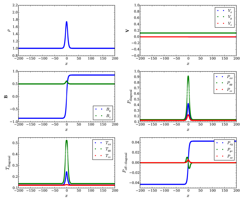
Figure 6: The results of a one-dimensional Riemann problem at $t=3500$, without gyrotropization and isotropization effects.

Once the redistribution of the thermal pressure is enforced through gyrotropization and/or isotropization, however, the imbalance again occurs. In the isotropic limit, in particular, the imbalance with $-B_{x}B_{y}$ can be resolved only through $V_{x}V_{y}$ since $P_{xy}=0$. Then, the induced $V_{x}$ drives the reconnection process, as we have already seen. Whether or not the reconnection is actually quenched in certain initial parameters, however, cannot be predicted until the Riemann problem is solved.

4.3 Field Loop Advection

The field loop advection problem is originally designed to test multidimensional MHD codes [11]. Since this problem contains a spacious, magnetically neutral region, it is suitable for investigating the capability to deal with an anisotropic pressure even in an unmagnetized region, which is one of the critical advantage of the present model.

In this problem, a weakly magnetized field loop is advected obliquely across the simulation domain $(x,y)\in[-L,L]\times[-L/2,L/2]$ with the velocity

$$\mathbf{V}=\left(V_{0},2V_{0},0\right),$$ (63)

which indicates that the field loop returns to the initial position after the time interval $t=2(L/V_{0})$. The magnetic field loop is given in the form of a vector potential by

$$A_{z}\left(x,y\right)=\left\{\begin{array}[]{ll}B_{0}\left(R-r\right)&\left(r\leq R\right)\\ 0&\left({\rm otherwise}\right)\end{array}\right.,$$ (66)

where $r=\sqrt{x^{2}+y^{2}}$ is the distance from the origin, $R=0.3L$ is the radius of the field loop, and $B_{0}$ is the magnetic field strength inside the loop. The magnetic field is initialized by taking a finite difference of the vector potential, otherwise a considerable error in $\nabla\cdot B$ will damage results seriously. The gas pressure is assumed to be isotropic and spatially uniform with $\beta=2\times 10^{6}$ inside the field loop. The density is also distributed uniformly, satisfying $P/\rho=V_{0}^{2}$. We adopt the normalization that $L$, $V_{0}$ and $B_{0}$ become unity. The computational domain is discretized with $400\times 200$ grid points. The effective collision frequency for gyrotropization is now set to be close to the dynamical time scale by assuming $\nu_{g}=10\left|\mathbf{B}\right|/B_{0}$.

The simulation result at the time when the field loop returns to the initial position is displayed in Fig.7. Four panels show (a) the magnetic pressure, (b) the magnetic field lines, (c) the deviation of the diagonally-averaged pressure from the uniform initial value, and (d) the in-plane, off-diagonal component of the pressure, respectively. All quantities are normalized by the initial magnetic pressure inside the field loop, $B_{0}^{2}/2$. Fig.7(a) is comparable to the top left panel in Fig.3 in [11], and well agrees with each other. From top two panels (a) and (b), related to the magnetic field, any spurious effects cannot be observed both inside the loop, where inadequate treatment of the electric field would result in a certain pattern, and at the vicinity of the edge of the loop, where the magnetic field changes discontinuously. We, therefore, conclude that the introduction of the pressure tensor induces no numerical difficulty in extension to multidimensional problems.

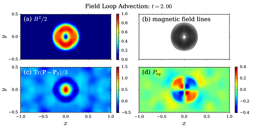
Figure 7: A snapshot at $t=2$ in the field loop advection problem. All variables are normalized by the initial magnetic pressure inside the field loop, $B_{0}^{2}/2$. Relatively slow gyrotropization is assumed with $\nu_{g}=10\left|B\right|/B_{0}$.

The bottom two panels (c) and (d) are related to the pressure tensor. Although the diagonally-averaged pressure, $\mathrm{Tr}\mathbf{P}/3$, is kept isotropic, a finite off-diagonal component, $P_{xy}$, makes a quadrupole pattern due to a difference between $P_{||}$ and $P_{\perp}$ inside the loop. Since the $xy$-component is given by $P_{xy}=(P_{||}-P_{\perp})\hat{b}_{x}\hat{b}_{y}$ under the assumption of a gyrotropic pressure, this pattern indicates the firehose-type anisotropy with $P_{||}>P_{\perp}$ by considering the direction of the magnetic field. Qualitatively speaking, this anisotropy can also be understood by the behavior based on the double adiabatic approximation, because the decomposition of the pressure tensor into parallel and perpendicular components is allowed inside the magnetic field loop. The intuitive form of the double adiabatic equations of states can be written as follows,

$$\frac{D}{Dt}\left(\frac{P_{\perp}}{\rho B}\right) = 0,$$ (67)

$$\frac{D}{Dt}\left(\frac{B^{2}P_{||}}{\rho^{3}}\right) = 0,$$ (68)

where $D/Dt=\partial/\partial t+\mathbf{V}\cdot\nabla$ indicates a Lagrangian derivative. Eqs. (67) and (68) indicate that the decrease of the magnetic field strength naturally leads to enhancement of the parallel pressure. In the present case, the magnetic field almost discontinuously changes across the outer edge of the field loop and also across the center of the loop, which results in the decrease of magnetic field strength through large numerical dissipation.

Finally, we emphasize that the present model can successfully solve the vast unmagnetized region in this problem without any numerical difficulty. The boundary between the magnetized and the unmagnetized regions are also captured seamlessly. Note that, except for an early stage, each cell might contain a non-zero magnetic field below or around the level of machine precision. Nevertheless, it may be no longer meaningful to define $P_{||}$ and $P_{\perp}$ there, and we strongly recommend the direct use of non-gyrotropic pressure tensor in essentially neutral regions.

4.4 Magnetorotational Instability

The previous tests involve only weak anisotropy that the resultant situation is stable to anisotropy-driven instabilities, i.e., firehose and mirror instabilities. In the case that one of these instabilities turns on, a rapidly growing eigenmode would severely break the simulation. This happens due to the fact that the growth rate becomes larger without bounds as the wavelength becomes shorter. The maximum growth rate of the kinetic counterpart of the MHD instability, on the other hand, will be limited by the finite Larmor radius effect. A compromise to avoid the disruption is presented in [34] (hereafter SHQS06). The authors limit the maximum degree of the pressure anisotropy by assuming that, once the anisotropy exceeds a threshold of one of the kinetic instabilities, the wave instantaneously reduces the anisotropy to the marginal state through pitch-angle scattering (hard wall limit). This model is applied to their simulations of magnetorotational instabilities (MRI) in a collisionless accretion disk based on the gyrotropic formulation and the Landau fluid model, and succeeds in tracking the non-linear evolution of the MRIs. In this subsection, we follow their pitch-angle scattering model and show the result of the MRI simulation as a test problem for highly non-linear evolution of an anisotropic plasma.

While the same thresholds (see Eqs. (32), (33), and (34) in SHQS06) are employed in the present test, we slightly modify the numerical procedure of the scattering model from SHQ06, where the collision terms in the equations of states, $\left[\partial P_{||}/\partial t\right]_{c}=-\left(2\nu/3\right)\left(P_{||}-P_{\perp}\right)$ and $\left[\partial P_{\perp}/\partial t\right]_{c}=-\left(\nu/3\right)\left(P_{\perp}-P_{||}\right)$, are solved implicitly. Instead of the implicit treatment, we use an analytic approach. Once the parallel and perpendicular pressure at a marginal state, $P_{||,s}$ and $P_{\perp,s}$, are determined, the analytic solution for the isotropized pressure tensor can also be obtained by solving

$$\left[\frac{\partial\mathbf{P}}{\partial t}\right]_{c}=-\nu_{\rm iso}\left(\mathbf{P}-\mathbf{P}_{s}\right),$$ (69)

where $\nu_{\rm iso}$ is an effective collision frequency of the pitch-angle scattering, which should be set to a much larger value than any dynamical frequencies of a system, and $\mathbf{P}_{s}$ is the marginal pressure tensor. For detail calculation of the marginal state, see B.

The other setup of our simulation is same as in SHQS06. With the help of the shearing box model [17, 36], the radial, azimuthal, and vertical coordinates in a cylindrical system are converted to $x$, $y$, and $z$ in a local Cartesian coordinate system, respectively, and the simulation domain is fixed to $(x,y,z)\in[-L/2,L/2]\times[0,2\pi L]\times[0,L]$, at the edges of which the so-called shearing periodic boundary conditions are employed. A differentially rotating plasma is, then, described by the shear velocity $\mathbf{V}_{0}=\left(0,-q\Omega_{0}x,0\right)$, where $\Omega_{0}$ is an angular velocity of a disk at the center of the simulation box, and a dimensionless parameter $q=-\ln\Omega/\ln R$ is set to be 1.5 in this paper. We assume that a plasma with the uniform and isotropic pressure, $\mathbf{P}=P_{0}\mathbf{I}$, is initially threaded by a weak vertical magnetic field with $\beta=400$. The initial mass density, $\rho_{0}$, is also uniform. To trigger off the growth of the MRIs, we add a random velocity perturbation with the magnitude of 0.1% of the isothermal sound speed, $c_{s}=\sqrt{P_{0}/\rho_{0}}$, which is equated to $\Omega L$ by assumption of a geometrically thin disk. In this problem, we employ the 5th-order WENO scheme and 3rd-order TVD Runge-Kutta scheme rather than 2nd-order methods for the purpose of resolving MRI-driven turbulence more accurately. The number of grid points is set to be $64\times 128\times 64$.

The time evolution of the volume-averaged energy density and the $xy$-component of the stress tensor, normalized by $P_{0}$, are shown in the top and bottom panels in Fig. 8, respectively.

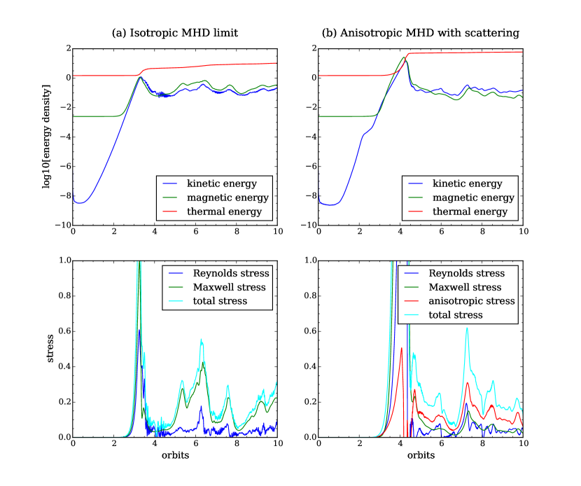
Figure 8: Volume-averaged energy density and stress normalized by an initial thermal pressure, as functions of time. Left two panels (a) show the results of an isotropic MHD limit, and right panels (b) the results of an anisotropic MHD with pitch-angle scattering models.

The results under the isotropic MHD limit are plotted in the left two panels for a comparison purpose, which show common behavior of the MRIs in unstratified shearing box simulations. In the early stage, all the unstable modes start exponential growth. After the fastest growing mode captured in the simulation box, whose wavelength is $\lambda=L/2$ in this case, becomes dominant, the non-linear growth of the longest wavelength mode with $\lambda=L$ soon forms a pair of inward and outward channel flows. As is well known, the amplitude of this channel flow structure continues to increase, since it is an exact solution of the shearing box system [12]. At roughly three orbits, the channel solution drastically breaks down into a turbulent state through the magnetic reconnection across the dense current sheet. On the saturated stage after that, the MHD turbulence continues to fill the simulation domain while repeating formation of local channel flows and the breakdowns by the reconnection. The kinetic energy in motion deviated from the Kepler orbit and the magnetic energy are in equipartition at this phase. The stress, however, is highly dominated by magnetic contribution, or the Maxwell stress. This large stress caused by MHD turbulence has been considered to play an important role for the angular momentum transport in the accretion disks. Note that the thermal energy keeps gradual increase, because the energy input into the simulation domain through the boundary condition finally dissipates to the thermal energy and no cooling mechanism is included in the system.

The anisotropic MHD calculation incorporated with the pitch-angle scattering model, on the other hand, leads to the right two plots in Fig. 8. There are two remarkable differences from the isotropic case in the energy history. One is a dent of the magnetic energy around two orbits. As described in SHQS06, this happens because the mirror-type pressure anisotropy with $P_{\perp}>P_{||}$ generated by the growth of the MRI suppresses the further growth of the MRI itself. If the scattering model is not included, the MRI stops at this level, and after that the simulation box will be filled with vertically propagating Alfvén waves.

The other major difference is the excessive peak of the magnetic energy around four orbits, just before the channel flow breaks down by magnetic reconnection. This feature was also pointed out in SHQS06, but not discussed with attention. For understanding this point, it is useful to consider the effect of the pressure anisotropy on the dynamics of magnetic reconnection as suggested in [24]. The author demonstrates the enhancement of the angular momentum transport in collisionless accretion disks by means of PIC simulations from the above point of view. They state that, although the mirror-type anisotropy with $P_{\perp}>P_{||}$ raised by the MRI is favorable for the reconnection, or tearing instabilities, to grow [6], the opposite firehose-type anisotropy with $P_{||}>P_{\perp}$ occurring in a dense current sheet as a result of reconnection will suppress further reconnection. The spatial distribution of the mass density and the pressure anisotropy observed in our calculation at the stage of the largest channel flow, $\Omega t/2\pi=4.2$, are shown in Fig. 9. The rightmost panel displaying the occurrence frequency as a function of $\rho$ and $P_{\perp}/P_{||}$ clearly shows that the inside of the dense current sheet is occupied with relatively isotropic or firehose-type anisotropic plasma compared with dilute lobe regions, which is consistent with the idea mentioned above. It is, however, not an obvious issue that whether or not the suppression and enhancement of a tearing instability in an anisotropic current sheet are captured in the present fluid model, either qualitatively or quantitatively. Further discussion is beyond the scope of this paper, and will be the subject of future work.

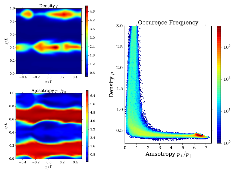
Figure 9: Slices of density and the pressure anisotropy distribution along $y=0$ at time $\Omega t/2\pi=4.2$, just before the largest channel flow structure breaks down. The rightmost panel shows an occurrence frequency as a function of the density and the anisotropy, which demonstrates that the dense current sheet consist of a relatively isotropic plasma or a slightly anisotropic plasma with $P_{||}>P_{\perp}$.

5 Summary and Conclusions

In this paper, we propose a natural extension of the double adiabatic approximation, or simply the CGL limit, to deal with the effect of an anisotropic pressure tensor in the framework of the magnetohydrodynamics. The features of our fluid model are summarized as follows:

1. All the six components of a pressure tensor are evolved according to Eq. (2), which is the 2nd-moment equation of the Vlasov equation without assuming isotropy or gyrotropy.

2. The effect of gyrotropization is introduced through an effective collision term with the collision rate proportional to the local magnetic field strength, which is a natural assumption from the physical insight into the last term of Eq. (2).

3. With the help of features 1. and 2., the present model successfully eliminates the singularity at a magnetic null point, to which the CGL equations cannot be applied.

4. By employing a large gyrotropization rate or a large isotropization rate, our model correctly reduces to the CGL limit (when a finite magnetic field exists) or the standard MHD, respectively, in an asymptotic manner.

The present model contains one free parameter, $\nu_{g}$, which controls the speed of gyrotropization. This time scale is, in general, considered to be much shorter than a dynamical time in a concerned system. In an (almost) unmagnetized region, however, such an ordering fails due to the lack of any cyclotron motion or due to a quite large gyro period, and hence, a singularity in the mathematical expression appears inevitably. Our fluid model can be recognized as one of the efforts to recover the regularity by adequately choosing the functional form of $\nu_{g}$ consistent with physical consideration of $\Omega_{c}\mathbf{P}\times\hat{\mathbf{b}}$ term in the 2nd-moment equation.

We also emphasize that it is an relatively easy task to extend an existing MHD code written in a conservative form to the present model, since we derive the basic equations as clear counterparts of the standard MHD. However, one should keep in mind that the effect of the directional energy exchange by Lorentz force cannot be grouped into the conservative term. This point requires an appropriate treatment for a Riemann solver as mentioned in Sec. 3; otherwise the calculation will fail to return a physically and mathematically consistent solution.

The prospective application of the present formulation includes wide variety of large-scale phenomena in collisionless plasmas, especially, where the effect of anisotropic pressure plays an important role. The magnetospheric plasma environment around the Earth is a typical example, in which the mean free path of charged particles and the typical spatial scale differ roughly by three orders of magnitude. Large temperature anisotropy has been measured by satellite observations, particularly, near the current sheets accompanied by magnetic reconnection [e.g., 25, 20, 2]. These magnetically neutral sites can also be solved seamlessly without any numerical and theoretical difficulties by this model.

Finally, focusing on the method to handle a pressure tensor, we neglect the moments of the Vlasov equation higher than two, such as heat fluxes. The establishment of a more sophisticated fluid model which can track other kinetic aspects is a highly challenging matter in the field of the collisionless plasma physics. The model proposed here may shed a light to this issue as a basis and as a guiding idea.

Appendix A Higer Order Implementation

In the text, our 2nd-order implementation is described in detail to clarify the differences from the standard MHD code. Here in this section, we give an example of more accurate implementation by employing spatially 5th-order scheme and temporally 3rd-order scheme.

In terms of the procedure in Sec. 3.4, step 2 is first replaced by the 5th-order WENO interpolation [27],

$$\mathbf{W}_{L,j+1/2}=w_{1}\mathbf{W}^{(1)}+w_{2}\mathbf{W}^{(2)}+w_{3}\mathbf{W}^{(3)},$$ (70)

where $\mathbf{W}^{(i)}$ represent the 3rd-order linear interpolation using different stencils,

$$\mathbf{W}^{(1)} = \frac{3}{8}\mathbf{W}_{j-2}-\frac{5}{4}\mathbf{W}_{j-1}+\frac{15}{8}\mathbf{W}_{j},$$ (71)

$$\mathbf{W}^{(2)} = -\frac{1}{8}\mathbf{W}_{j-1}+\frac{3}{4}\mathbf{W}_{j}+\frac{3}{8}\mathbf{W}_{j+1},$$ (72)

$$\mathbf{W}^{(3)} = \frac{3}{8}\mathbf{W}_{j}+\frac{3}{4}\mathbf{W}_{j+1}-\frac{1}{8}\mathbf{W}_{j+2}.$$ (73)

The normalized nonlinear weights, $w_{i}=\hat{w}_{i}/(\hat{w}_{1}+\hat{w}_{2}+\hat{w}_{3})$, are chosen to reduce to small numbers around discontinuities as

$$\hat{w}_{i}=\frac{\gamma_{i}}{(\beta_{i}+10^{-6})^{2}},$$ (74)

with the optimum weights

$$\gamma_{1}=\frac{1}{16},\ \ \gamma_{2}=\frac{5}{8},\ \ \gamma_{3}=\frac{5}{16},$$ (75)

which ensure the convergence to the 5th-order linear interpolation in smooth regions. $\beta_{i}$ is called the global smoothness indicator [30], which is the weighted average of the smoothness indicator for each variable,

$$\beta_{i}=\frac{1}{N_{d}}\sum_{d=1}^{N_{d}}\frac{\beta^{d}_{i}}{||W^{d}||^{2}},$$ (76)

where $N_{d}=13$ indicates the number of independent variables, and $\beta_{r}^{d}$ is the smoothness indicator for $d$-th variable, defined as

$$\beta_{1}^{d} = \frac{13}{12}\left(W_{j-2}^{d}-2W_{j-1}^{d}+W_{j}^{d}\right)^{2}+\left(\frac{W_{j-2}^{d}-4W_{j-1}^{d}+3W_{j}^{d}}{2}\right)^{2},$$ (77)

$$\beta_{2}^{d} = \frac{13}{12}\left(W_{j-1}^{d}-2W_{j}^{d}+W_{j+1}^{d}\right)^{2}+\left(\frac{W_{j-1}^{d}-W_{j+1}^{d}}{2}\right)^{2},$$ (78)

$$\beta_{3}^{d} = \frac{13}{12}\left(W_{j}^{d}-2W_{j+1}^{d}+W_{j+2}^{d}\right)^{2}+\left(\frac{3W_{j}^{d}-4W_{j+1}^{d}+W_{j+2}^{d}}{2}\right)^{2}.$$ (79)

By using the reversed stencils, $\mathbf{W}_{R,j-1/2}$ can also obtained in the same way. Note that the coefficients described here are not for reconstruction, but for interpolation. Employing the interpolation scheme as a point value enables us to use various kind of Riemann solvers in the finite difference approach as well, and to couple the scheme with the CT method.

Next, the conversion from a point-value flux to a numerical flux must be carried out for $\mathbf{F}_{L,R}$ and $\mathbf{D}_{L,R}$ before taking two-point differences in step 7. This can be achieved by comparing the coefficients in Taylor expansion[35]. The 6th-order formula, for example, is obtained as

$$\hat{\mathbf{f}}_{j\pm 1/2}=\mathbf{f}_{j\pm 1/2}-\frac{\Delta x^{2}}{24}\left.\frac{\partial^{2}\mathbf{f}}{\partial x^{2}}\right|_{j\pm 1/2}+\frac{7\Delta x^{4}}{5760}\left.\frac{\partial^{4}\mathbf{f}}{\partial x^{4}}\right|_{j\pm 1/2}.$$ (80)

The 2nd- and 4th-derivatives are evaluated by the simple central differences with 4th- and 2nd-order of accuracy, respectively, which guarantee the 6th-order of accuracy in total.

The derivatives for non-conservative terms using the minmod limiter in step 7 must also be replaced by the higher order one. In our implementation, the face-centered values, $\mathbf{U}_{L,j+1/2}$ and $\mathbf{U}_{R,j-1/2}$, are calculated from the cell-centered values, $\mathbf{U}_{j}$, as numerical fluxes by the WENO scheme as well as in step 2. In this case, however, the coefficients are adjusted for reconstruction, since we do not need the reconstructed value elsewhere. Now Eqs. (71) to (73) are modified as

$$\mathbf{U}^{(1)} = \frac{1}{3}\mathbf{U}_{j-2}-\frac{7}{6}\mathbf{U}_{j-1}+\frac{11}{6}\mathbf{U}_{j},$$ (81)

$$\mathbf{U}^{(2)} = -\frac{1}{6}\mathbf{U}_{j-1}+\frac{5}{6}\mathbf{U}_{j}+\frac{1}{3}\mathbf{U}_{j+1},$$ (82)

$$\mathbf{U}^{(3)} = \frac{1}{3}\mathbf{U}_{j}+\frac{5}{6}\mathbf{U}_{j+1}-\frac{1}{6}\mathbf{U}_{j+2}.$$ (83)

The optimum weights also change to

$$\gamma_{1}=\frac{1}{10},\ \ \gamma_{2}=\frac{3}{5},\ \ \gamma_{3}=\frac{3}{10}.$$ (84)

The use of these coefficients ensures that the two-point difference,

$$\left.\frac{\partial\mathbf{U}}{\partial x}\right|_{j}\simeq\frac{1}{\Delta x}\left(\mathbf{U}_{L,j+1/2}-\mathbf{U}_{R,j-1/2}\right),$$ (85)

has 5th-order of accuracy in smooth regions, while showing non-osclillatory behavior around discontinuities.

Finally, the 2nd-order time integration (36) and (37) is replaced by 3rd-order TVD Runge-Kutta method [35]:

$$\mathbf{U}^{(1)} = \mathbf{U}^{n}-\Delta t\mathcal{L}\left(\mathbf{U}^{n}\right),$$ (86)

$$\mathbf{U}^{(2)} = \frac{3}{4}\mathbf{U}^{n}+\frac{1}{4}\left[\mathbf{U}^{(1)}-\Delta t\mathcal{L}\left(\mathbf{U}^{(1)}\right)\right],$$ (87)

$$\mathbf{U}^{n+1} = \frac{1}{4}\mathbf{U}^{n}+\frac{2}{3}\left[\mathbf{U}^{(2)}-\Delta t\mathcal{L}\left(\mathbf{U}^{(2)}\right)\right].$$ (88)

Appendix B Isotropization Model

In the present paper, the hard-wall limit employed in [34] is modified to use the analytic solution of Eq. (69), or explicitly,

$$\mathbf{P}^{n+1}=\mathbf{P}_{s}+\left(\mathbf{P}^{n}-\mathbf{P}_{s}\right)e^{-\nu_{\rm iso}\Delta t},$$ (89)

where $\mathbf{P}_{s}$ is a marginal state of a certain kinetic instability. For the firehose, mirror, and ion-cyclotron instabilities, the following relations are satisfied, respectively:

$$\frac{P_{\perp,s}}{P_{||,s}}-1+\frac{B^{2}}{P_{||,s}} = -\frac{1}{2},$$ (90)

$$\frac{P_{\perp,s}}{P_{||,s}}-1 = \frac{\xi B^{2}}{P_{\perp,s}},$$ (91)

$$\frac{P_{\perp,s}}{P_{||,s}}-1 = S\left(\frac{B^{2}}{P_{||,s}}\right)^{1/2},$$ (92)

where $\xi=3.5$ and $S=0.3$ are used in this paper. Each equation can be solved for $P_{||,s}$ and $P_{\perp,s}$ if we impose the condition that the total thermal energy, which is proportional to a trace of the pressure tensor, is unchanged through the scattering, i.e., the relation $P^{n}_{||}+2P^{n}_{\perp}=P_{||,s}+2P_{\perp,s}$ holds. Note that this condition exactly guarantees the energy conservation, $\mathrm{Tr}\mathbf{P}^{n+1}=\mathrm{Tr}\mathbf{P}^{n}$. In the case that the firehose instability turns on, for example, solving Eq. (90) leads to

$$P_{||,s} = \mathrm{Tr}\mathbf{P}^{n}+2B^{2},$$ (93)

$$P_{\perp,s} = \frac{\mathrm{Tr}\mathbf{P}^{n}}{2}-B^{2}.$$ (94)

The marginal states for the mirror and ion-cyclotron instabilities can also be calculated in the same way.

To avoid duplicated gyrotropization, it may be better to construct the marginal pressure tensor in a non-gyrotropic form. We adopt, therefore, the following prescription,

$$\mathbf{P}_{s}=\mathbf{R}\left(\begin{array}[]{ccc}\hat{P}_{11,s}&0&0\\ 0&\alpha\hat{P}^{n}_{22}&\alpha\hat{P}^{n}_{23}\\ 0&\alpha\hat{P}^{n}_{32}&\alpha\hat{P}^{n}_{33}\end{array}\right)\mathbf{R}^{T},$$ (98)

where $\mathbf{R}$ is a rotational matrix from the coordinate system aligned with a local magnetic field to the $xyz$-coordinate system, $\hat{P}_{ij}\ (i,j=1,2,3)$ is a pressure component measured in the field-aligned coordinates (the parallel direction is assumed as $i=1$), $\hat{P}_{11,s}=P_{||,s}$, and $\alpha=P_{\perp,s}/P^{n}_{\perp}$. The convergence to this marginal state allows the pressure to keep finite non-gyrotropy, while the thermal energy contained in the parallel and perpendicular components are correctly redistributed.

References

- Amano [2015] Amano, T. (2015). Divergence-free Approximate Riemann Solver for the Quasi-neutral Two-fluid Plasma Model. Journal of Computational Physics, 299, 863–886.
- Artemyev et al. [2015] Artemyev, A. V., Petrukovich, A. A., Nakamura, R., & Zelenyi, L. M. (2015). Statistics of intense dawn-dusk currents in the Earth’s magnetotail. Journal of Geophysical Research (Space Physics), 120, 3804–3820.
- Brio & Wu [1988] Brio, M., & Wu, C. C. (1988). An upwind differencing scheme for the equations of ideal magnetohydrodynamics. Journal of Computational Physics, 75, 400–422.
- Burch et al. [2015] Burch, J. L., Moore, T. E., Torbert, R. B., & Giles, B. L. (2015). Magnetospheric Multiscale Overview and Science Objectives. Space Science Review, .
- Chandran et al. [2011] Chandran, B. D. G., Dennis, T. J., Quataert, E., & Bale, S. D. (2011). Incorporating Kinetic Physics into a Two-fluid Solar-wind Model with Temperature Anisotropy and Low-frequency Alfvén-wave Turbulence. The Astrophysical Journal, 743, 197.
- Chen & Palmadesso [1984] Chen, J., & Palmadesso, P. (1984). Tearing instability in an anisotropic neutral sheet. Physics of Fluids, 27, 1198–1206.
- Chew et al. [1956] Chew, G. F., Goldberger, M. L., & Low, F. E. (1956). The Boltzmann Equation and the One-Fluid Hydromagnetic Equations in the Absence of Particle Collisions. Proceedings of the Royal Society of London Series A, 236, 112–118.
- Dumbser & Balsara [2016] Dumbser, M., & Balsara, D. S. (2016). A new efficient formulation of the HLLEM Riemann solver for general conservative and non-conservative hyperbolic systems. Journal of Computational Physics, 304, 275–319.
- Dumin [2002] Dumin, Y. V. (2002). The corotation field in collisionless magnetospheric plasma and its influence on average electric field in the lower atmosphere. Advances in Space Research, 30, 2209–2214.
- Evans & Hawley [1988] Evans, C. R., & Hawley, J. F. (1988). Simulation of magnetohydrodynamic flows - A constrained transport method. The Astrophysical Journal, 332, 659–677.
- Gardiner & Stone [2005] Gardiner, T. A., & Stone, J. M. (2005). An unsplit Godunov method for ideal MHD via constrained transport. Journal of Computational Physics, 205, 509–539.
- Goodman & Xu [1994] Goodman, J., & Xu, G. (1994). Parasitic instabilities in magnetized, differentially rotating disks. The Astrophysical Journal, 432, 213–223.
- Hada et al. [1999] Hada, T., Jamitzky, F., & Scholer, M. (1999). Consequences of nongyrotropy in magnetohydrodynamics. Advances in Space Research, 24, 67–72.
- Harten et al. [1983] Harten, A., Lax, P. D., & van Leer, B. (1983). On Upstream Differencing and Godunov-Type Schemes for Hyperbolic Conservation Laws. SIAM Review, 25, 1–149.
- Hau & Sonnerup [1993] Hau, L.-N., & Sonnerup, U. O. (1993). On slow-mode waves in an anisotropic plasma. Geophysical Research Letters, 20, 1763–1766.
- Hau & Wang [2007] Hau, L.-N., & Wang, B.-J. (2007). On MHD waves, fire-hose and mirror instabilities in anisotropic plasmas. Nonlinear Processes in Geophysics, 14, 557–568.
- Hawley et al. [1995] Hawley, J. F., Gammie, C. F., & Balbus, S. A. (1995). Local Three-dimensional Magnetohydrodynamic Simulations of Accretion Disks. The Astrophysical Journal, 440, 742.
- Heinemann [1999] Heinemann, M. (1999). Role of collisionless heat flux in magnetospheric convection. Journal of Geophysical Research, 104, 28397–28410.
- Hesse et al. [2004] Hesse, M., Kuznetsova, M., & Birn, J. (2004). The role of electron heat flux in guide-field magnetic reconnection. Physics of Plasmas, 11, 5387–5397.
- Hietala et al. [2015] Hietala, H., Drake, J. F., Phan, T. D., Eastwood, J. P., & McFadden, J. P. (2015). Ion temperature anisotropy across a magnetotail reconnection jet. Geophysical Review Letters, 42, 7239–7247.
- Hirabayashi & Hoshino [2013] Hirabayashi, K., & Hoshino, M. (2013). Magnetic reconnection under anisotropic magnetohydrodynamic approximation. Physics of Plasmas, 20, 112111.
- Hollweg [1976] Hollweg, J. V. (1976). Collisionless electron heat conduction in the solar wind. Journal of Geophysical Research, 81, 1649–1658.
- Holzer et al. [1971] Holzer, T. E., Fedder, J. A., & Banks, P. M. (1971). A comparison of kinetic and hydrodynamic models of an expanding ion-exosphere. Journal of Geophysical Research, 76, 2453.
- Hoshino [2015] Hoshino, M. (2015). Angular Momentum Transport and Particle Acceleration During Magnetorotational Instability in a Kinetic Accretion Disk. Physical Review Letters, 114, 061101.
- Hoshino et al. [1997] Hoshino, M., Saito, Y., Mukai, T., Nishida, A., Kokubun, S., & Yamamoto, T. (1997). Origin of hot and high speed plasmas in plasma sheet: plasma acceleration and heating due to slow shocks. Advances in Space Research, 20, 973–982.
- Ichimaru [1977] Ichimaru, S. (1977). Bimodal behavior of accretion disks - Theory and application to Cygnus X-1 transitions. The Astrophysical Journal, 214, 840–855.
- Jiang & Shu [1996] Jiang, G.-S., & Shu, C.-W. (1996). Efficient Implementation of Weighted ENO Schemes. Journal of Computational Physics, 126, 202–228.
- Karimabadi et al. [2014] Karimabadi, H., Roytershteyn, V., Vu, H. X., Omelchenko, Y. A., Scudder, J., Daughton, W., Dimmock, A., Nykyri, K., Wan, M., Sibeck, D., Tatineni, M., Majumdar, A., Loring, B., & Geveci, B. (2014). The link between shocks, turbulence, and magnetic reconnection in collisionless plasmas. Physics of Plasmas, 21, 062308.
- Kowal et al. [2011] Kowal, G., Falceta-Gonçalves, D. A., & Lazarian, A. (2011). Turbulence in collisionless plasmas: statistical analysis from numerical simulations with pressure anisotropy. New Journal of Physics, 13, 053001.
- Levy et al. [2000] Levy, D., Puppo, G., & Russo, G. (2000). Compact Central WENO Schemes for Multidimensional Conservation Laws. SIAM Review, 22, 656–672.
- Londrillo & del Zanna [2004] Londrillo, P., & del Zanna, L. (2004). On the divergence-free condition in Godunov-type schemes for ideal magnetohydrodynamics: the upwind constrained transport method. Journal of Computational Physics, 195, 17–48.
- Narayan & Yi [1994] Narayan, R., & Yi, I. (1994). Advection-dominated accretion: A self-similar solution. The Astrophysical Journal, 428, L13–L16.
- Quataert [2003] Quataert, E. (2003). Radiatively Inefficient Accretion Flow Models of Sgr A*. Astronomische Nachrichten Supplement, 324, 435–443.
- Sharma et al. [2006] Sharma, P., Hammett, G. W., Quataert, E., & Stone, J. M. (2006). Shearing Box Simulations of the MRI in a Collisionless Plasma. The Astrophysical Journal, 637, 952–967.
- Shu & Osher [1988] Shu, C.-W., & Osher, S. (1988). Efficient Implementation of Essentially Non-oscillatory Shock-Capturing Schemes. Journal of Computational Physics, 77, 439–471.
- Stone & Gardiner [2010] Stone, J. M., & Gardiner, T. A. (2010). Implementation of the Shearing Box Approximation in Athena. The Astrophysical Journal Supplement Series, 189, 142–155.
- Stone et al. [2008] Stone, J. M., Gardiner, T. A., Teuben, P., Hawley, J. F., & Simon, J. B. (2008). Athena: A New Code for Astrophysical MHD. The Astrophysical Journal Supplement Series, 178, 137–177.
- Tóth [2000] Tóth, G. (2000). The Constraint in Shock-Capturing Magnetohydrodynamics Codes. Journal of Computational Physics, 161, 605–652.
- Wang et al. [2015] Wang, L., Hakim, A. H., Bhattacharjee, A., & Germaschewski, K. (2015). Comparison of multi-fluid moment models with particle-in-cell simulations of collisionless magnetic reconnection. Physics of Plasmas, 22, 012108.
- Zouganelis et al. [2004] Zouganelis, I., Maksimovic, M., Meyer-Vernet, N., Lamy, H., & Issautier, K. (2004). A Transonic Collisionless Model of the Solar Wind. The Astrophysical Journal, 606, 542–554.