String networks with junctions in competition models

Abstract

In this work we give specific examples of competition models, with six and eight species, whose three-dimensional dynamics naturally leads to the formation of string networks with junctions, associated with regions that have a high concentration of enemy species. We study the two- and three-dimensional evolution of such networks, both using stochastic network and mean field theory simulations. If the predation, reproduction and mobility probabilities do not vary in space and time, we find that the networks attain scaling regimes with a characteristic length roughly proportional to $t^{1/2}$, where $t$ is the physical time, thus showing that the presence of junctions, on its own, does not have a significant impact on their scaling properties.

Physics Letters A pla Physics Letters A 2011Published by Elsevier Ltd.

1 Introduction

Competition models are widely regarded as a crucial tool to understand the mechanisms leading to biodiversity [1, 2, 3, 4] (see also [5, 6] for a review). Although the simplest competition models usually consider three species and allow for an equal number of basic microscopic actions (motion, reproduction and predation), many interesting generalizations, including further species and more complex interaction rules, have been considered in the literature [7, 8, 9, 10, 11, 12, 13, 14, 15, 16, 17, 18, 19, 20, 21, 22, 23, 24, 25, 26, 27, 28, 29, 30, 31]

In [14, 15], a broad family of spatial stochastic May-Leonard models with an arbitrary number of species has been introduced. There, many interesting features of this family of models, including the dynamics of complex networks of spiralling patterns and interfaces, have been investigated in detail. Recently, in [25], it has been shown that specific sub-classes of this family of models may lead to the emergence of string networks in three spatial dimensions. These strings are associated to predator-prey interactions which occur mainly along lines corresponding to a high concentration of enemy species. The strings studied in [25] do not have junctions and their dynamics has been shown to be curvature driven.

In this paper we consider the emergence of string networks with junctions in the context of specific spatial stochastic competition models belonging to the general family introduced in [14, 15]. We investigate the two- and three-dimensional dynamics of these models using both stochastic and mean field network simulations. The outline of this paper is as follows. In Set. 2 we introduce a sub-class of stochastic May-Leonard models allowing for the formation of string networks with junctions in three spatial dimensions. In Sec. 3 we investigate the stochastic evolution of two- and three-dimensional networks in models belonging to the above sub-class with $N=6$ or $N=8$ species. In Sec. 4 we study the dynamics of such systems using mean field theory simulations, considering also the particular case of the collapse of a circular loop. In Sec. 5 we constrain the scaling parameter $\lambda$ governing the macroscopic dynamics of these models, considering various choices for the mobility, predation and reproduction parameters. Finally, we conclude in Sec. 6.

2 Family of models

Here, we consider a sub-class of the more general family of spatial stochastic May-Leonard models introduced in Refs. [14, 15]. We investigate models with an even number of species $N>4$, where each species competes with $N-4$ other species. The competition diagrams for the simplest cases with $N=6$ and $N=8$ species are illustrated in the left and right panels of Fig. 1, respectively. The double arrows indicate that the predation between competing species is bi-directional. Except for the labelling of the different species, the diagrams depicted in Fig. 1 are invariant under rotations by $\theta_{n}=2\,\pi(n/N)$, with $n=0,\pm 1,\pm 2,\dots,\pm(N-1)$, indicating the presence of a $Z_{N}$ symmetry.

In these models individuals of $N$ species are initially distributed on square or cubic lattices with ${\mathcal{N}}$ sites. The different species are labeled by $i=1,\ldots,N$, and the cyclic identification $i=i+k\,N$, where $k$ is an integer, is made. The sum of the number of individuals of the species $i$ ($I_{i}$) with the number of empty sites ($I_{E}$) is equal to the total number of sites (${\mathcal{N}}$), that is

$$\sum_{i=1}^{N}I_{i}+I_{E}={\mathcal{N}}.$$ (1)

At each time step a random individual (active) is chosen to interact with one of its nearest neighbours (passive), also selected randomly. The number of neighbours is equal to four, in the case of the two-dimensional square lattice, and to six, in the case of the three-dimensional cubic lattice. The unit of time $\Delta t=1$ is defined as the time necessary for ${\mathcal{N}}$ interactions to occur (one generation). The possible interactions are classified as Motion $i\ \odot\to\odot\ i\,,$ Reproduction $i\ \otimes\to ii\,,$ or Predation $i\ \ (i\pm\alpha)\to i\ \otimes\,,$ where $\odot$ may be any species ($i$) or an empty site ($\otimes$) and $\alpha=1,\ldots,(N-4)/2$. A constant predation probability $p$ between competing species, and constant reproduction and mobility probabilities ($r$ and $m$, respectively), common to all species, is considered. Although this class of models is defined for a generic even $N>4$, in this paper we shall investigate explicitly the models illustrated in Fig. 1, with $N=6$ and $N=8$ different species.

3 Stochastic network simulations

We performed a series of stochastic network simulations of the models with six and eight species in two and three spatial dimensions (in square and cubic lattices, respectively). The numerical results show that, as soon as the simulations start, individuals of the same species, originally distributed randomly throughout the lattice, share common spatial regions. The individuals tend not to be close to competitors, but in the vicinity of individuals of the same species or of other neutral species.

Figure 1: Diagrams describing the possible predator-prey interactions in the models with $N=6$ (left panel) and $N=8$ (right panel) different species.

Figure 2: Illustration of a defect/anti-defect pair with four species in a model with an arbitrary number of species $N$, where $i=1,...,\frac{N}{2}$.

In two spatial dimensions such spatial configurations promote the coexistence of species which may be organized either clockwise or counterclockwise, around roughly circular regions with a significantly higher density of empty sites. Attacks and counter-attacks between competing species on opposite sides of the battle cores ensure the stability of such spatial patterns. Similar two-dimensional arrangements of the species have been found in Ref. [25]. These can be described as defect/anti-defect configurations associated to clockwise/counterclockwise vortex states, respectively. The average area of the defect and anti-defect cores depends on the interaction probabilities ($m$, $p$, $r$), but it is roughly constant in time.

In contrast with the model described in Ref. [25], where every species would compete with $N-3$ distinct ones, here each species has less competitors (each species has $N-4$ competitors and three neutral species). As a consequence, the number of configurations which promote coexistence among species is enlarged. In fact, while in Ref. [25] all $N$ species have to be gathered around the defect cores in order to guarantee their stability, here, a stable defect configuration requires only four species. Defects/anti-defects arise when the different species dispose themselves in the clockwise/counterclockwise vortex configurations shown in Fig. 2 $\{i,i+\frac{N}{2},i+1,i-\frac{N-2}{2}\}$, where $i=1,...,\frac{N}{2}$ (note that each species $i$ does not interact with the species $i\pm\frac{N-2}{2}$ and $i+\frac{N}{2}$). These configurations account for $\frac{N}{2}$ different kinds of defect/anti-defects with four species.

Consider the competing species $i$ and $i+1$ belonging to the defect/anti-defect configuration shown in Fig. 2. The average number of attacks per unit time from individuals of the outer species $i+1$ supersedes those from individuals of the inner species $i$. This implies that individuals of the outer species tend to invade the territory of the inner ones causing an approximation and annihilation of the defect/anti-defect pair. We shall show that the defect/anti-defect cores attract each other, having a velocity which is, on average, inversely proportional to the distance between them. In contrast, a pair of clockwise (or counterclockwise) defects (anti-defects) cannot annihilate and repel each other.

Moreover, defect/anti-defect configurations with a larger number of species may arise. In fact, defect/anti-defect configurations with $n=4,...,\frac{N+2}{2}$ species, in which each species competes with $n-3$ other species, may appear in models with an even number $N>6$ of species.

All network simulation snapshots presented throughout this paper were obtained by assuming $m=0.10$, $p=0.80$ and $r=0.10$. Although these values were found to be adequate for visualization purposes, we verified that many other choices of the parameters would provide similar qualitative results.

3.1 6 species

Let us focus on the simplest case with $N=6$. The left panel of Fig. 3 shows one snapshot taken from a two-dimensional $1024^{2}$ stochastic network simulation with periodic boundary conditions. Each grid point is at most occupied by one individual which belongs to the species indicated by the same color as in Fig. 1. In addition, empty spaces are represented by white dots.

Figure 3: Snapshots obtained from two-dimensional $1024^{2}$ stochastic network simulations of the $N=6$ (left panel) and $N=8$ (right panel) models. The color scheme used here is the same as represented in Fig. 1 for $i=1$.

The spatial patterns show that all defects involve four different species. Most of the predator-prey interactions take place at the defect core, which is surrounded by two pairs of competing domains, each domain being dominated by a single species. More specifically, one may identify three types of defects-anti/defects where domains dominated by the species $\{i,i-1,i+1,i-2\}$ (where $i=1,2,3$) arrange themselves in this order (or the reverse) around the defect (anti-defect) cores. Due to the periodic boundary conditions, the number of defects in each simulation is equal to the number of anti-defects. As the network evolves, the number of defects becomes increasingly smaller due to the annihilation of defect/anti-defect pairs. Ultimately, at large enough $t$, only one group of three species which do not compete each other may survive (either $(1,3,5)$ or $(2,4,6)$), and the symmetry of the model is said to be spontaneously broken.

We also run a series of $256^{3}$ three-dimensional stochastic network simulations with periodic boundary conditions of the $N=6$ model. We notice that the extension to three spatial dimensions of the dynamics presented in the left panel of Fig. 3 gives rises to a string network with Y-type junctions. Such strings represent regions with a significant larger number density of empty spaces, which appear as a consequence of the frequent predation interaction between competing species taking place at their core.

The snapshot shown in the left panel of Fig. 4 represents a $64^{3}$ region of the entire $256^{3}$ three-dimensional lattice. It presents the contour plots associated to a fixed value of the density of empty sites, which highlight the presence of a string network with junctions (note that, in order to improve the visualization, the number density of empty spaces has been convolved with a gaussian filter function).

Figure 4: Snapshots taken from a three-dimensional $64^{3}$ region of a $256^{3}$ stochastic network simulation of the $N=6$ (left panel) and $N=8$ (right panel) models.

Throughout their evolution the strings intersect and intercommute (exchange partners). This process is responsible for the production of string loops which collapse with a characteristic velocity roughly proportional to the loop characteristic scale. The collapse of a string loop is curvature driven and it is associated to the existence of a defect/anti-defect pair on any plane intersecting the loop. The loop collapse will be further considered in Sec. 4.3.

Since any planar defect or anti-defect involves only four species, each species joins two different strings in three spatial dimensions. This is responsible for the appearance of Y-type junctions, defined as the meeting point of three different strings. The stability of the junctions is ensured by predator-prey interactions, given that each species has competitors in two different strings.

The upper panel of Fig. 5 illustrates the different possible configurations of a string junction in the $N=6$ model, where $i=1,2,3$. Note that, in this model, all the species are involved in the formation of a Y-type junctions, each one of them being associated to two different strings.

3.2 8 species

The results obtained for $N=8$ are qualitatively similar to those presented for $N=6$, but with an increased complexity associated with the larger number of species. In this case, apart from the four different defects/anti-defects with four species represented by $\{i,i+4,i+1,i-3\}$ (where $i=1,..4$), there are eight defect/anti-defect configurations composed by five species. They are composed by the clockwise/counterclockwise disposition of the species $\{i,i+4,i+1,i-2,i+3\}$ (where $i=1,..8$) around the defect cores. We call the defects formed by four and five species, type I and II, respectively.

The right panel of Fig. 3 depicts one snapshot taken from a $1024^{2}$ stochastic network simulation of the $N=8$ model, with periodic boundary conditions. The colors indicate the species that individuals belong to (See Fig. 1). White dots represent empty sites.

In addition, the results provided by three-dimensional simulations are presented in the right panel of Fig. 4. The snapshot represents a $64^{3}$ region of a three-dimensional $256^{3}$ stochastic network simulations with periodic boundary conditions of the $N=8$ model.

Figure 5: Illustration of the formation of Y-type junctions in the models $N=6$ (left panel) and $N=8$ (right panel). The cross-sections of the different types of strings joining the junctions are presented, where $i=1,...,\frac{N}{2}$.

Analogously to the $N=6$ model, the extension to three spatial dimensions gives rises to a string network with junctions. Nonetheless, in the $N=8$ model there are two different types of strings, in which either four (type I) or five different species (type II) are involved. One string of type I and two of type II are required in order to produce the stable Y-type junctions seen in the simulations of the $N=8$ model. The lower panel of Fig. 5 illustrates the formation of a Y-type junction in this model.

4 Mean field theory simulations

Let us define $N+1$ scalar fields ($\phi_{0}$, $\phi_{1}$, $\phi_{2}$, $\ldots$, $\phi_{N}$) representing the fraction of space around a given point occupied by empty sites ($\phi_{0}$) and by individuals of the species $i$ ($\phi_{i}$), satisfying the constraint $\phi_{0}+\phi_{1}+\ldots+\phi_{N}=1$. For an even $N>4$ the mean field equations of motion

$${\dot{\phi}}_{0} = D\nabla^{2}\phi_{0}-r\phi_{0}\sum_{i=1}^{N}\phi_{i}+p\,\sum_{i=1}^{N}\,\left(\sum_{\alpha=1}^{\frac{N-4}{2}}\phi_{i}\phi_{i+\alpha}+\sum_{\alpha=\frac{N+4}{2}}^{N-1}\phi_{i}\phi_{i+\alpha}\right)\,,$$ (2)

$${\dot{\phi}}_{i} = D\nabla^{2}\phi_{i}+r\phi_{0}\phi_{i}-p\left(\sum_{\alpha=1}^{\frac{N-4}{2}}\phi_{i}\phi_{i+\alpha}+\sum_{\alpha=\frac{N+4}{2}}^{N-1}\phi_{i}\phi_{i+\alpha}\right)\,,$$ (3)

describe the average dynamics of the models studied in the previous section (see [7], for more details). Here, a dot represents a derivative with respect to the physical time and $D=2m$ is the diffusion rate.

4.1 Two and three-dimensional numerical results

Figure 6 depicts two snapshots taken from $1024^{2}$ mean field network simulations with periodic boundary conditions of the $N=6$ (left panel) and $N=8$ (right panel) models. Initial conditions with $\phi_{i}=1$ if $i=s$ and $\phi_{i}=0$ if $i\neq s$ were set at each grid point ($\phi_{0}$ was set to zero at every grid point). Here $s$ is a species drawn randomly at each grid point.

The results provided by the mean field simulations (Fig. 6) are similar to those obtained from the stochastic network evolution (Fig. 3), except for the noise (the color scheme is the same in both figures). This correspondence also occurs in the three-dimensional simulations. In particular, the macroscopic dynamics depicted in the snapshot shown in Fig. 7 obtained from three-dimensional $256^{3}$ mean field theory simulations of the $N=6$ and $N=8$ models, is similar (again, except for the noise) to that shown in Fig. 4.

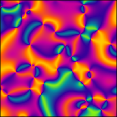
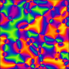
Figure 6: Snapshots obtained from two-dimensional $1024^{2}$ mean field simulations of the $N=6$ (left panels) and $N=8$ (right panels) models.

4.2 Defect profile

Let us now consider the defect profiles, i.e., the stationary number density of empty spaces in and around the defect cores. In other words, let us study the spatial distribution of $\phi_{0}$ around a defect center, considering that the defect has radial symmetry and is centered at $r=0$.

Furthermore, we aim to understand the dependence of the defect profile on the parameters ($m$, $p$, $r$). To this purpose, we consider three different models characterized by a domination of motion [model $M$: ($m$, $p$, $r$)=(0.8, 0.1, 0.1)], predation [model $P$: ($m$, $p$, $r$)= (0.1, 0.8, 0.1)] or reproduction [model $R$: ($m$, $p$, $r$) = (0.1, 0.1, 0.8)] interactions.

Figure  8 shows the value of $\phi_{0}$, as a function of the distance $r$ to the defect core, obtained for defects associated with four and five species from mean field simulations of the $N=6$ (upper panel) and $N=8$ (middle and lower panels) models. The disposition of the species around the defect cores is shown in the inset plots.

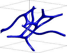
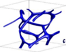
Figure 7: Snapshots taken from three-dimensional mean field simulations of the $N=6$ (left panel) and $N=8$ (right panel) models. The figures represent $64^{3}$ regions of $256^{3}$ simulations.

The numerical results show a strong dependence of the defect profile on the model parameters. Specifically, the defect profile height is larger in the case of model P, dominated by predation interactions. On the contrary, a larger reproduction rate leads to a smaller number density of empty spaces (model $R$). Finally, a larger mobility parameter leads to the broadening of the defect profile, since the individuals are more likely to move outside the core of the defect into enemy territory (model $M$).

Figure  8 also shows that, in the model with $N=8$ species and for fixed ($m$, $p$, $r$), the defect is broader when the number of species composing the defect is increased from $4$ to $5$.

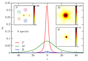
Figure 8: Defect profiles obtained for defects with four and five species from mean field simulations for $N=6$ (left panel) and $N=8$ (right and lower panels). The inset plots represent the disposition of the species around the defect cores.

4.3 String loop

We now investigate the collapse of a circular string loop using mean field theory simulations in a cubic lattice. To identify the string we define a new variable $\varphi({\vec{r}},t)\equiv{\rm max}(\phi_{0}({\vec{r}},t))-\phi_{0}^{c},0)$. Here, $\phi_{0}^{c}$ represents a threshold which guarantees that only grid points with a high number density of empty sites, close to the core of the string, are identified as belonging to the string. The average number density of empty sites associated to the string is then defined by

$$\rho(t)=\frac{1}{{\cal N}^{2}}\sum_{\vec{r}}\varphi({\vec{r}},t)\,.$$ (4)

We recall that the average number of empty sites per unit string length ($\mu$) does not change significantly with time. Therefore, the loop perimeter is proportional to $\rho(t)$ and the area of the string loop $a(t)$ evolves proportionally to $\rho^{2}(t)$.

The time evolution of the area $a(t)$ of the circle enclosed by the loop is determined using mean field theory simulations in a $256^{3}$ cubic lattice. We run simulations for two different threshold values in order to ensure the accuracy and reliability of the results. The upper panel of Fig.  9 displays the evolution of the area of a string loop formed by four distinct species $a_{4}(t)$ in the $N=6$ model. Note that the results are almost identical for both choices of threshold values, $\phi_{0}^{c}=0.06$ and $\phi_{0}^{c}=0.15$, which correspond approximately to $25\%$ and $60\%$ of the maximum of $\phi_{0}$ ($\phi_{0}^{max}$) at the core of the string. Similar results were found for the evolution of area of the circle enclosed by string loops associated to four and five distinct species $a_{4}(t)$ and $a_{5}(t)$ in the $N=8$ model (see lower panel of Fig.  9). Fig.  9 shows that the loop area decreases linearly in time according to

$$a(t)=a_{0}\left(1-\frac{t}{t_{c}}\right)\ ,$$ (5)

where $t_{c}$ is the collapse time or, equivalently, that radius of curvature decreases proportionally to $t^{1/2}$. A similar result has been obtained in Ref. [15] for a different model allowing for string networks without junctions.

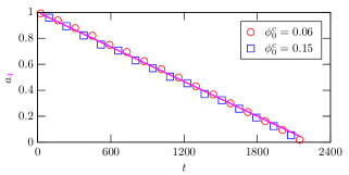
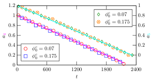
Figure 9: Mean field evolution of the areas of string loops in the $N=6$ (left panel) and $N=8$ (right panel) models, computed by taking different threshold values. Note that $a_{4}(t)$ and $a_{5}(t)$ represent the areas of type I and type II string loops, respectively.

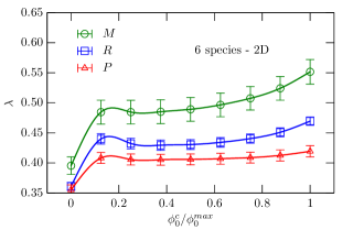
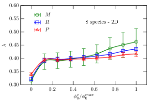
Figure 10: The dependence of the scaling exponent $\lambda$ on the threshold $\phi_{0}^{c}$ in a mean field simulation with $N=6$ (left panel) and $N=8$ (right panel) species. The results were obtained by carrying out $10$ simulations of $2048^{2}$ two-dimensional networks for a wide range of $\phi_{0}^{c}$, for models $M$, $P$ and $R$. The error bars represent the standard deviation in an ensemble of 10 simulations.

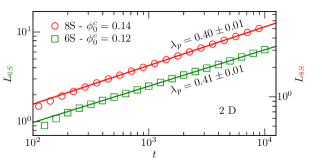
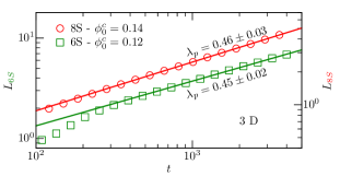
Figure 11: Scaling behavior for the models with $N=6$ and $N=8$ different species obtained using $2048^{2}$ two-dimensional (left panel) and $256^{3}$ three-dimensional (right panel) mean field numerical simulations.

5 Scaling behavior

Finally, we consider the scaling behavior of the models investigated in the previous sections using mean field theory simulations. To this purpose, let us define the characteristic length $L$ of the defect network as

$$L=\sqrt{\frac{\mu}{\rho}}\propto\sqrt{\frac{1}{\rho}}\ ,$$ (6)

where $\mu$ is the average number of empty spaces associated with the defects (per unit string length, in three spatial dimensions) and $\rho$ is the average number density of empty sites associated to the defect network defined by Eq. (4).

By fitting a scaling law $L\propto t^{\lambda}$, we constrain the evolution of the characteristic length of the string network with time for different sets of $10$ mean field simulations of the models $M$, $R$ and $P$. Each simulation starts with different random initial conditions.

The upper and lower panels of Fig.  10 show the dependence of $\lambda$ on the threshold $\phi_{0}^{c}$ for models $M$, $P$ and $R$, for $N=6$ and $N=8$, respectively (in units of $\phi_{0}^{c}/\phi_{0}^{max}$). For $N=8$, $\phi_{0}^{max}$ is taken as the maximum of $\phi_{0}$ at the core of the string of type I. The error bars represent the standard deviation in an ensemble of 10 simulations. Figure  10 shows that if the $\phi_{0}^{c}$ is between $20\%$ and $60\%$ of $\phi_{0}^{max}$, the scaling constant $\lambda$ does not show a significant dependence on the threshold. Outside this interval, this is no longer the case. For lower values of $\phi_{0}^{c}$, this happens because low density regions far away from the core are being taken as belonging to the defect. On the other hand, the number of lattice points associated with the defect may become too small for higher values of $\phi_{0}^{c}$.

The average evolution of $L$ with time $t$ was obtained for sets of 10 distinct two- and three-dimensional mean field network simulations ($2048^{2}$ and $256^{3}$) with random initial conditions. Fig.  11 shows that the characteristic lengths $L_{6S}$ (6 species) and $L_{8S}$ (8 species) evolve in reasonable agreement with the scaling law $L\propto t^{\lambda}$, with $\lambda=1/2$, characteristic of networks in which the dynamics is curvature driven. Here, the points denote the average value of $L$ computed from the simulation and the error bars provide information on the root-mean-square deviation for each set of $10$ simulations. In all cases the value of $L$ was normalized to unity at $t=100$, the parameters ($m$, $p$, $r$) were set to (0.10, 0.80, 0.10) and the threshold $\phi_{0}^{c}$ was fixed at $40\%$ of $\phi_{0}^{max}$ (for $N=8$ the treshold $\phi_{0}^{c}$ was obtained by considering the value of $\phi_{0}^{max}$ obtained for type II strings).

These results are consistent with those obtained in Ref. [25] for models allowing for string networks without junctions in three spatial dimensions. A similar behavior may also be found in other physical systems, in particular in the case of curvature driven dynamics of string networks in condensed matter.

6 Comments and Conclusions

In this work we have shown that there are specific sub-classes, with an even number of species, of a more general family of May-Leonard models which lead to the formation of cosmic string networks with junctions, associated to regions with a high concentration of empty spaces. We have investigated the dynamics of these networks using stochastic and mean field network simulations, assuming that the predation, reproduction and mobility probabilities are constant in space and time. We have found that the presence of junctions does not have a significant impact on the scaling behaviour of the characteristic macroscopic scale of the network $L$ with the physical time $t$, showing that it grows roughly proportional to $t^{1/2}$. We have also shown that our results are not strongly dependent on the specific values of the mobility, predation or reproduction probabilities.

Our findings are expected to be relevant not only for the evolution of biological populations in three spatial dimensions but also for the understanding of the evolution of cosmic string networks with junctions in other contexts. In particular, in [32] one investigates bifurcation and pattern changing in the relativistic regime, suggesting how to solve the cosmological domain wall problem. Also, in [33] it has been shown that, although the evolution of the characteristic macroscopic length and velocity of interface networks with physical time in relativistic and non-relativistic regimes is very different, single snapshots with the same characteristic scale do not clearly differentiate between these two regimes. Hence, our results may also be relevant for the understanding of the dynamical behaviour of complex relativistic defect networks with junctions in a cosmological setting (e.g. cosmic superstrings [34, 35, 36]).

References

- [1] B. Kerr, M. A. Riley, M. W. Feldman, B. J. M. Bohannan, Mobility promotes and jeopardizes biodiversity in rock–paper–scissors games, Nature 418 (2002) 171.
- [2] J. J. Leisner, J. Haaber, Intraguild predation provides a selection mechanism for bacterial antagonistic compounds, Proceedings of the Royal Society B: Biological Sciences 279 (2012) 4513.
- [3] H. Cheng, N. Yao, Z. Huang, J. Park, Y. Do, Y. Lai, Mesoscopic interactions and species coexistence in evolutionary game dynamics of cyclic competitions, Scientific Reports 4 (2014) 7486.
- [4] A. J. Daly, J. M. Baetens, B. D. Baets, The impact of initial evenness on biodiversity maintenance for a four-species in silico bacterial community, Journal of Theoretical Biology 387 (2015) 189 – 205.
- [5] R. C. Sole, J. Bascompte, Self-Organization in Complex Ecosystems, Princeton UP, Princeton, 2006.
- [6] M. A. Nowak, Evolutionary Dynamics: Exploring the Equations of Life, Harvard University Press, 2006.
- [7] R. May, W. Leonard, Nonlinear aspects of competition between three species, SIAM Journal on Applied Mathematics 29 (1975) 243.
- [8] T. Reichenbach, M. Mobilia, E. Frey, Mobility promotes and jeopardizes biodiversity in rock–paper–scissors games, Nature 448 (2007) 1046.
- [9] T. Reichenbach, M. Mobilia, E. Frey, Noise and correlations in a spatial population model with cyclic competition, Phys. Rev. Lett. 99 (2007) 238105.
- [10] M. Peltomaki, M. Alava, Three- and four-state rock-paper-scissors games with diffusion, Phys. Rev. E 78 (2008) 031906.
- [11] W.-X. Wang, X. Ni, Y.-C. Lai, C. Grebogi, Pattern formation, synchronization, and outbreak of biodiversity in cyclically competing games, Phys. Rev. E 83 (2011) 011917.
- [12] A. Dobrinevski, E. Frey, Extinction in neutrally stable stochastic lotka-volterra models, Phys. Rev. E 85 (2012) 051903.
- [13] A. Roman, D. Konrad, M. Pleimling, Cyclic competition of four species: domains and interfaces, Journal of Statistical Mechanics: Theory and Experiment (2012) P07014.
- [14] P. P. Avelino, D. Bazeia, L. Losano, J. Menezes, von neummann’s and related scaling laws in rock-paper-scissors-type games, Phys. Rev. E 86 (2012) 031119.
- [15] P. P. Avelino, D. Bazeia, L. Losano, J. Menezes, B. F. Oliveira, Junctions and spiral patterns in generalized rock-paper-scissors models, Phys. Rev. E 86 (2012) 036112.
- [16] A. Roman, D. Dasgupta, M. Pleimling, Interplay between partnership formation and competition in generalized may-leonard games, Phys. Rev. E 87 (2013) 032148.
- [17] J. Vukov, A. Szolnoki, G. Szabó, Diverging fluctuations in a spatial five-species cyclic dominance game, Phys. Rev. E 88 (2013) 022123.
- [18] A. Dobrinevski, M. Alava, T. Reichenbach, E. Frey, Mobility-dependent selection of competing strategy associations, Phys. Rev. E 89 (2014) 012721.
- [19] C. Rulquin, J. J. Arenzon, Globally synchronized oscillations in complex cyclic games, Phys. Rev. E 89 (2014) 032133.
- [20] P. P. Avelino, D. Bazeia, L. Losano, J. Menezes, B. F. de Oliveira, Interfaces with internal structures in generalized rock-paper-scissors models, Phys. Rev. E 89 (2014) 042710.
- [21] B. Szczesny, M. Mobilia, A. M. Rucklidge, Characterization of spiraling patterns in spatial rock-paper-scissors games, Phys. Rev. E 90 (2014) 032704.
- [22] L. Varga, J. Vukov, G. Szabó, Self-organizing patterns in an evolutionary rock-paper-scissors game for stochastic synchronized strategy updates, Phys. Rev. E 90 (2014) 042920.
- [23] S. Mowlaei, A. Roman, M. Pleimling, Spirals and coarsening patterns in the competition of many species: a complex ginzburg–landau approach, Journal of Physics A: Mathematical and Theoretical 47 (16) (2014) 165001.
- [24] C. S. Gokhale, A. Traulsen, Evolutionary multiplayer games, Dynamic Games and Applications 4 (4) (2014) 468–488.
- [25] P. P. Avelino, D. Bazeia, J. Menezes, B. de Oliveira, String networks in lotka–volterra competition models, Physics Letters A 378 (4) (2014) 393 – 397.
- [26] A. Szolnoki, M. Perc, Vortices determine the dynamics of biodiversity in cyclical interactions with protection spillovers, New Journal of Physics 17 (11) (2015) 113033.
- [27] M. F. Weber, G. Poxleitner, E. Hebisch, E. Frey, M. Opitz, Chemical warfare and survival strategies in bacterial range expansions, Journal of The Royal Society Interface 11 (96) (2014) 20140172.
- [28] D. Grošelj, F. Jenko, E. Frey, How turbulence regulates biodiversity in systems with cyclic competition, Phys. Rev. E 91 (2015) 033009.
- [29] B. Intoy, M. Pleimling, Synchronization and extinction in cyclic games with mixed strategies, Phys. Rev. E 91 (2015) 052135.
- [30] G. Szabó, K. S. Bodó, B. Allen, M. A. Nowak, Four classes of interactions for evolutionary games, Phys. Rev. E 92 (2015) 022820.
- [31] A. Roman, D. Dasgupta, M. Pleimling, A theoretical approach to understand spatial organization in complex ecologies, Journal of Theoretical Biology 403 (2016) 10 – 16.
- [32] P. P. Avelino, D. Bazeia, R. Menezes, J. C. R. E. Oliveira, Bifurcation and pattern changing with two real scalar fields, Phys. Rev. D 79 (2009) 085007.
- [33] P. P. Avelino, R. Menezes, J. C. R. E. Oliveira, Unified paradigm for interface dynamics, Phys. Rev. E 83 (2011) 011602. doi:10.1103/PhysRevE.83.011602.
- [34] E. J. Copeland, R. C. Myers, J. Polchinski, Cosmic F- and D-strings, Journal of High Energy Physics 6 (2004) 013.
- [35] M. G. Jackson, N. T. Jones, J. Polchinski, Collisions of cosmic F- and D-strings, Journal of High Energy Physics 10 (2005) 013.
- [36] L. Sousa, P. P. Avelino, Probing cosmic superstrings with gravitational waves, Phys. Rev. D 94 (2016) 063529.