Generalized Wishart processes for interpolation over diffusion tensor fields

Abstract

Diffusion Magnetic Resonance Imaging (dMRI) is a non-invasive tool for watching the microstructure of fibrous nerve and muscle tissue. From dMRI, it is possible to estimate 2-rank diffusion tensors imaging (DTI) fields, that are widely used in clinical applications: tissue segmentation, fiber tractography, brain atlas construction, brain conductivity models, among others. Due to hardware limitations of MRI scanners, DTI has the difficult compromise between spatial resolution and signal noise ratio (SNR) during acquisition. For this reason, the data are often acquired with very low resolution. To enhance DTI data resolution, interpolation provides an interesting software solution. The aim of this work is to develop a methodology for DTI interpolation that enhance the spatial resolution of DTI fields. We assume that a DTI field follows a recently introduced stochastic process known as a generalized Wishart process (GWP), which we use as a prior over the diffusion tensor field. For posterior inference, we use Markov Chain Monte Carlo methods. We perform experiments in toy and real data. Results of GWP outperform other methods in the literature, when compared in different validation protocols.

1 Introduction

Diffusion Magnetic Resonance Imaging (dMRI) is a non-invasive procedure to find connections into biological mediums such as fiber nerves and muscle tissue. From dMRI it is possible to estimate the apparent diffusivity coefficient (ADC) of water particles within tissue by solving the Stejskal-Tanner formulation [5]. A 2-rank diffusion tensor $(D)$ is employed to modeling ADC in each specific voxel, where $D$ is a symmetric and positive definite $3\times 3$ matrix. Following this notion, a diffusion tensor imaging (DTI) field is understood as a grid of individual but related diffusion tensors. Although a DTI field shows how some nerve fiber bundles are interconnected, there are some limitations in MRI scanners. For example, dMRI is sensitive to the difficult compromise between spatial resolution and signal to noise ratio (SNR). This leads to data acquisitions with low resolution [16].

To enhance DTI data resolution, interpolation provides an interesting and feasible methodological solution. Diffusion tensor fields belong to a Riemannian space, where the Riemannian metric is defined by the inner product assigned to each point of this space. With this metric, one can to compute geodesic distances between diffusion tensors and to calculate different statistics in this space [8]. An important condition is keeping the smooth transition of anisotropic features inherent in the given tensor fields (i.e. Fractional anisotropy-FA maps), especially around degenerate points, where at least two of three eigenvalues are equivalent [6]. Interpolation of the diffusion tensor fields have many applications. For example, registration of DTI datasets will require resolution enhancement when a registration transformation is applied to a tensor field. Other examples that require DTI interpolation include segmentation, atlas construction, diagnosis of neurological diseases, etc [3]. Currently, the clinical acquisition protocols of dMRI data allow one or two millimeters resolution for each voxel. The problem here, is that brain tissue fiber bundles are in micrometers scale. Therefore, the tractography models developed from DTI data can be imprecise due to the current low resolution in acquired images. Normally, visualization of DTI is discrete, where it is used ellipsoids or glyphs for graphic representation. Tractography is the search of fiber connection among neighboring voxels. The basic idea is to generate a continuous data representation [9]. According to this, an accurate interpolation approach may improve the spatial resolution of diffusion tensor fields in a considerable factor. Therefore, the tractography process will describe with more detail the fiber tissue connection.

Some recent works have proposed interpolation methods for tensor fields in DTI. They developed a variety of mathematical approaches, such as: direct smooth approximation [13] and euclidean approaches, but they do not retain the principal properties of a DTI, i.e positive definite tensors. For this reason, the scientific community has been looking alternative methods for estimating tensor fields that keep the symmetric positive definite (SPD) constraint inside the grid of tensors. [1] presented a Log-euclidean approximation and [8] developed a Riemannian framework achieving important advances in tensor fields geometry, but they lack in smoothness property in presence or high level of noise. [3] presented a b-spline scheme that interpolates SPD tensors with high accuracy using the Riemannian metric. The authors introduced a tensor product of B-splines that minimizes the Riemannian distance between tensors. Following the Riemannian framework, [10] presented Geodesic-loxodromes that can identify isotropic and anisotropic components of the tensor and interpolates each component separately. Finally, alternative methodologies have been posited: a tensor field reconstruction based on eigenvector and eigenvalue interpolation [9], location of degenerated lines in 2-D planar [6], and a feature-based interpolation [17]. However, those methods do not achieve an adequate representation of a DTI field obtained from noisy real data.

As previously was pointed out, most of the methods for DTI interpolation are based on Riemannian geometry. While they preserve the main properties of DTI data, and solve limitations of the Euclidean approaches, they lead to rigid interpolations that fail to fully adapt to the variety of diffusion patterns in biological tissues [7]. In this work, we present a novel methodology for interpolation of DTI fields. Instead of a Riemann geometry framework, we propose a stochastic modeling of DTI. We assume that a DTI field follows a generalized Wishart process (GWP). A GWP is a collection of symmetric positive definite random matrices indexed by an arbitrary dependent variable [15], i.e. the $x,y,z$ position. In this context, we use it to model the entire DTI field $D(x,y,z)$. Then, through approximate Bayesian inference (i.e Elliptical slice sampling and Markov Chain Monte Carlo methods), we estimate the optimal parameters of the model. Stochastic modeling of DTI fields has some advantages: positive definite matrices, robustness to noise, smooth transition among nearby tensors and good accuracy for estimating new data. We compare our approach with linear interpolation [13] and a Riemannian method known as log-euclidean interpolation [1]. We perform experiments in toy and real DTI data. Results of GWP improve to the comparison methods in different validation protocols.

2 Materials and methods

2.1 DTI estimation from dMRI and DTI fields

Diffusion Magnetic Resonance Imaging (dMRI) studies the diffusion of water particles in the human brain. Diffusion can be described by a symmetric positive definite $3\times 3$ matrix proportional to the covariance of a Gaussian distribution [5, 14].

$$\textbf{D}=\begin{bmatrix}{D_{xx}}&{D_{xy}}&{D_{xz}}\\ {D_{yx}}&{D_{yy}}&{D_{yz}}\\ {D_{zx}}&{D_{zy}}&{D_{zz}}\end{bmatrix}$$

For water, the diffusion tensor (DT) is symmetric, so that $D_{ij}=D_{ji}$, where $i,j=x,y,z$. The diffusion tensor for each voxel of the dMRI is calculated using the Stejskal-Tanner formulation [5]:

$$S_{k}=S_{0}e^{-b\hat{\mathbb{g}}_{k}^{\top}D\hat{\mathbb{g}}_{k}},$$ (1)

where $S_{k}$ is the $k^{th}$ dMRI, $S_{0}$ is the reference image, $\hat{\mathbb{g}}_{k}$ is the gradient vector and $b$ is the diffusion coefficient. At least $7$ dMRI measurements are necessary for each slice ($k=0,1,...,7$). Usually, DTI fields are estimated from (1) using least squares [4]. However, there are robust methods for DT estimation. In this work, we use the RESTORE algorithm [11] for solving the DTs.

Traditionally, rank-2 DTs have been visualized by constructing the ellipsoid given by:

$$\mathbf{r}^{\top}D^{-1}\mathbf{r}=C$$ (2)

where $\mathbf{r}^{\top}=[x,y,z]$ is the position vector, and $C$ is a constant with the units of time. Therefore, the resulting shape is a level surface of the expression on the left side of (2), and it is possible to show by diagonalization that these surfaces are ellipsoids.

2.2 Generalized Wishart Process (GWP)

We begin with the Wishart distribution, which defines a probability density function over a symmetric positive definite matrix. Let $S$ be a $p\times p$ symmetric positive definite matrix of random variables. Let $V$ be a (fixed) positive definite matrix of size $p\times p$. Then, if $\nu\geq p$, $S$ has a Wishart distribution with $\nu$ degrees of freedom if it has a probability density function given by:

$$S=\frac{|S|^{\nu-p-1}}{2^{\nu p/2}|V|^{\nu/2}\Gamma_{p}(\frac{\nu}{2})}e^{-\frac{1}{2}\operatorname{trace}(V^{-1}S)},$$

where $|\cdot|$ is the determinant and $\Gamma_{p}$ is the multivariate gamma function:

$$\Gamma_{p}\left(\frac{\nu}{2}\right)=\pi^{\frac{p(p-1)}{4}}\prod_{j=1}^{p}\Gamma\left(\frac{\nu}{2}+\frac{1-j}{2}\right)$$

Following this notion and according to the definition given in [15], a generalized Wishart process (GWP) is as a collection of symmetric positive definite random matrices indexed by an arbitrary and high dimensional dependent variable $\mathbf{z}$. In DTI fields, the dimension is $p=3$ because diffusion tensors are represented by $3\times 3$ matrices, and the indexed variable refers to position coordinates $\textbf{z}=[x,y,z]^{\top}$. Assume $3\nu$ independent Gaussian process functions $u_{id}(\mathbf{z})\sim\mathcal{GP}(0,k)$, for $i=1,...,\nu$ and $d=1,2,3$, where $k(\mathbf{z},\mathbf{z}^{\prime})$ is the covariance or kernel function for the GP. Given a set of input vectors $\{\mathbf{z}\}_{n=1}^{N}$, the vector $(u_{id}(\mathbf{z}_{1}),u_{id}(\mathbf{z}_{2}),...,u_{id}(\mathbf{z}_{N}))^{\top}\sim\mathcal{N}(\mathbf{0},K)$, being $K$ an $N\times N$ Gram matrix with entries $K_{ij}=k(\mathbf{z}_{i},\mathbf{z}_{j})$. If we define $\hat{\mathbf{u}}_{i}(\mathbf{z})=\left(u_{i1}(\mathbf{z}),u_{i2}(\mathbf{z}),u_{i3}(\mathbf{z})\right)^{\top}$ and $L$ as the lower Cholesky decomposition of a $p\times p$ scale matrix $V$, such that $LL^{\top}=V$, for each input position $\mathbf{z}=[x,y,z]^{\top}$, the diffusion tensor $D(\mathbf{z})$ follows a Wishart distribution,

$$D(\mathbf{z})=\sum_{i=1}^{\nu}L\hat{\mathbf{u}}_{i}(\mathbf{z})\hat{\mathbf{u}}^{\top}_{i}(\mathbf{z})L^{\top}\sim\mathcal{GWP}_{p}(\nu,V,k(\cdot,\cdot)),$$ (3)

In this work, we use the squared exponential kernel $k(\mathbf{z},\mathbf{z^{\prime}})$,

$$k(\mathbf{z},\mathbf{z^{\prime}})=\exp\left(-0.5\frac{\lVert\mathbf{z}-\mathbf{z^{\prime}}\rVert^{2}}{\theta^{2}}\right),$$

where $\theta$ is the length-scale hyperparameter.

2.3 Bayesian inference for DTI field learning

In order to perform DTI interpolation, we first need to compute the posterior distribution for the variables in the model. For a DTI field, we assume a prior given by a Generalized Wishart process

$$p\left(D(\mathbf{z})\right)\sim\mathcal{GWP}_{3}(\nu,V,k(\cdot,\cdot))=\displaystyle\sum_{i=1}^{\nu}L\hat{\mathbf{u}}_{i}(\mathbf{z})\hat{\mathbf{u}}_{i}^{\top}(\mathbf{z})L^{\top}.$$ (4)

For the likelihood function, we assume each element from the diffusion tensor data follows an independent Gaussian distribution with the same variance $\sigma^{2}$. This leads to a likelihood with the following form:

$$p(S|u,L,\nu)\propto\prod_{i=1}^{N}\exp\left(-\frac{1}{2\sigma^{2}}\lVert S(\mathbf{z}_{i})-D(\mathbf{z}_{i})\rVert_{frob}^{2}\right),$$

where $S(\mathbf{z})$ is the known initial DTI field with low resolution, $D(\mathbf{z})$ is constructed from equation (4), and Frobenius norm is given by

$$\lVert\mathbf{X}\rVert_{frob}^{2}=\operatorname{trace}\left(\mathbf{X}^{T}\mathbf{X}\right).$$

The purpose is to infer the posterior probability of $D(\mathbf{z})$ given a known tensorial data set $S(\mathbf{z})=\{S(\mathbf{z}_{1}),S(\mathbf{z}_{2}),...,S(\mathbf{z}_{N})\}$, being $N$ the number of data in the initial DTI field. We first compute the posterior of the relevant variables in equation (4) including the vector of all GP function values $\mathbf{u}$, length-scale hyperparameter of the GP kernel function $\theta$, the lower Cholesky decomposition of the scale matrix $L$, such that $LL^{\top}=V$, and the degrees of freedom $\nu$. Given a GWP prior for the model and the likelihood function, the posterior distributions can be computed by

$$p(\mathbf{u}|\theta,L,S)\propto p(S|\mathbf{u},L,\nu)p(\mathbf{u}|\theta),$$ (5)

$$p(\theta|\mathbf{u},L,S)\propto p(\mathbf{u}|\theta,L,D)p(\theta),$$ (6)

$$p(L|\mathbf{u},\theta,S)\propto p(S|\mathbf{u},L,\nu)p(L).$$ (7)

We use Markov chain Monte Carlo algorithms to sample in cycles. We employ Metropolis-Hastings to sample $\theta$ from (6), and the elements of scale matrix $L$ from (7). To sample $\mathbf{u}$ from (5), we employ elliptical slice sampling [12]. We choose $\nu=5$ through cross-validation. We set a log-normal prior on $\theta$, a spherical Gaussian prior on elements of $L$ and the prior $p(\mathbf{u}|\theta)\sim\mathcal{N}(\mathbf{0},K_{B})$ is a Gaussian distribution with $3\nu N\times 3\nu N$ block diagonal covariance matrix $K_{B}$, formed using $3\nu$ of the $K$ matrices.

2.4 DTI field interpolation through GWP modeling

Once we find the posterior distributions over all relevant variables for the model, we can compute the posterior distribution for $D(\mathbf{z}_{*})$ in a new spatial position $\mathbf{z}_{*}=[x_{*},y_{*},z_{*}]^{\top}$. First, we have to infer the distribution over all unknown GP function values $\mathbf{u}_{*}$ in $\mathbf{z}_{*}$, where $\mathbf{u}_{*}$ is a vector with elements given by $u_{id}(\mathbf{z}_{*})$. The joint distribution over $\mathbf{u}$ and $\mathbf{u}_{*}$ is given by,

$$\begin{bmatrix}{\mathbf{u}}\\ {\mathbf{u}_{*}}\end{bmatrix}\sim\mathcal{N}\left(\mathbf{0},\begin{bmatrix}{K_{B}}&{A^{\top}}\\ {A}&{I_{p}}\end{bmatrix}\right)$$

If $\mathbf{u}_{*}$ and $\mathbf{u}$ have $p$ and $q$ elements respectively, $A$ is a $p\times q$ matrix that represents the covariances between $\mathbf{u}_{*}$ and $\mathbf{u}$ for all pairs of training and validation data, this is $A_{ij}=k_{i}(\mathbf{z}_{*},\mathbf{z}_{j})$ for $i+(i-1)N\leq j\leq iN$, and $0$ otherwise. $I_{p}$ is a $p\times p$ identity matrix. Using the properties of a Gaussian distribution, and conditioning on $\mathbf{u}$, we obtain:

$$p\left(\mathbf{u}_{*}|\mathbf{u}\right)\sim\mathcal{N}\left(AK_{B}^{-1}\mathbf{u},I_{p}-AK_{B}^{-1}A^{\top}\right)$$ (8)

From values of $\mathbf{u}_{*}$ obtained from (8), and using equation (3), we can construct $D(\mathbf{z}_{*})$.

2.5 Validation procedure and datasets

As ground truth (gold standard) we employ three different types of data. The first one corresponds to a synthetic DTI field. The second one corresponds to a simulation of crossing fibers using the algorithm of the fanDTasia toolBox [2], available at http://www.cise.ufl.edu/~abarmpou/lab/fanDTasia/. The third one, corresponds to a DTI dataset estimated from real dMRI through the RESTORE method [11]. dMRI data of the head were acquired from a healthy subject on a General Electric Signa HDxt 3.0T MR scanner using the body coil for excitation, and an 8-channel quadrature brain coil for reception. We employ $25$ gradient directions with a value for b equal to $1000$ $S/mm^{2}$. The study contains $128\times 128\times 33$ images in axial plane. For the three datasets, we downsample the DTI field by a factor of two. The downsampled field is the input data for the GWP. After we perform inference over the GWP, we interpolate the DTI field, and calculate two error metrics, having the gold standards as our references. Also, we repeat the same procedure for linear [13] and log-euclidean interpolation [1] for a comparison with two commonly used methods in the state of the art. We use two metrics to measure the differences between the interpolated fields and the ground truth, the Frobenius norm, and the Riemman distance, defined by

$$\operatorname{Frob}(T_{1},T_{2})=\sqrt{\operatorname{trace}\left[\left(T_{1}-T_{2}\right)^{\top}\left(T_{1}-T_{2}\right)\right]},$$

$$\operatorname{Riem}(T_{1},T_{2})=\sqrt{\operatorname{trace}\left[\log(T_{1}^{-1/2}T_{2}T_{1}^{-1/2})^{\top}\log(T_{1}^{-1/2}T_{2}T_{1}^{-1/2})\right]},$$

where $T_{1}$ and $T_{2}$ are the estimated and the ground truth tensors, respectively. The error metrics are computed for each voxel. We report the mean and standard deviation for the errors over the predicted data.

3 Experimental results and discussion

In this section, we present the interpolation results for the different DTI datasets. We compare with linear [13] and log-euclidean interpolation [1].

3.1 Synthetic Data

We generate noisy random DTI data to construct a $2D$ field of $37\times 37$ tensors. We assume $25$ gradient directions for generating DTs, and $b$ value of $1000$ $s/mm^{2}$. In Figure 1 we can see the initial downsampled DTI field, linear and log-euclidean interpolation, the interpolated field with GWP, and the ground truth respectively. Table 1 shows the error metrics.

(a)

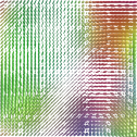
(b)

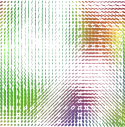
(c)

(d)

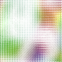
(e)

Figure 1: Graphic results for DTI interpolation $(2\times)$ applied in synthetic data. (a) Downsampled DTI field (data used for estimation). (b) Linear interpolation. (c) Log-euclidean interpolation. (d) Interpolation with GWP. (e) Ground truth.

Table 1: Metric results for synthetic DTI field

	Frobenius distance $(\times 10^{-5})$	Riemman distance
GWP	$7.06\pm 1.51$	$0.160\pm 0.125$
linear interpolation	$50.11\pm 4.26$	$8.54\pm 1.36$
log-euclidean	$35.25\pm 3.92$	$6.34\pm 1.22$

3.2 DTI from crossing fibers

One of the most critical DTI datasets correspond to crossing fibers. We generate this type of DTI field through FanDTasia toolbox [2]. This dataset describes a $2D$ crossing fiber field with $31\times 31$ tensors. Figure 2 and Table 2 show the comparative results.

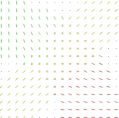
(a)

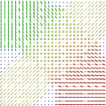
(b)

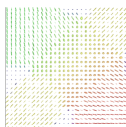
(c)

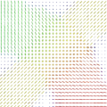
(d)

(e)

Figure 2: Graphic results for DTI interpolation $(2\times)$ applied in crossing fibers field. (a) Downsampled DTI field (data used for estimation). (b) Linear interpolation. (c) Log-euclidean interpolation. (d) Interpolation with GWP. (e) Ground truth.

Table 2: Error measures for crossing fibers in a DTI field.

	Frobenius distance $(\times 10^{-5})$	Riemman distance
GWP	$18.11\pm 11.82$	$0.184\pm 0.114$
linear interpolation	$73.12\pm 8.26$	$11.14\pm 2.65$
log-euclidean	$61.09\pm 6.15$	$9.74\pm 1.67$

3.3 Real DTI field estimated from dMRI

Finally, we test our method in real DTI data estimated from dMRI acquired in a human subject. The field corresponds to an axial slice with $49\times 55$ tensors. Figure 3 and Table 3 show the comparative results.

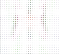
(a)

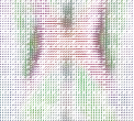
(b)

(c)

(d)

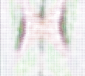
(e)

Figure 3: Graphic results for DTI interpolation $(2\times)$ applied in real DTI data. (a) Downsampled DTI field (data used for estimation). (b) Linear interpolation. (c) Log-euclidean interpolation. (d) Interpolation with GWP. (e) Ground truth.

Table 3: Error measures for the real DTI field example

	Frobenius distance $(\times 10^{-5})$	Riemman distance
GWP	$6.26\pm 3.20$	$0.146\pm 0.080$
linear interpolation	$45.76\pm 7.21$	$7.25\pm 2.10$
log-euclidean	$31.67\pm 6.10$	$6.89\pm 1.86$

3.4 Discussion

Linear and log-euclidean interpolation seek to minimize geodesic distances. The geometric (Riemann and Euclidean) approaches work well in smooth DTI fields. However, they reduce their performance in presence of high level of noise. For example, when we interpolate the synthetic noisy data (Figure 1 and Table 1), we can observe a swelling effect for the estimated tensors in the new input locations, when using linear interpolation. This is a critical issue, because this effect modifies the fractional anisotropy maps. Another big problem with linear interpolation is the possibility of obtaining non-positive definite tensors. Although, non-positive definite tensors are avoided with log-euclidean interpolation, the accuracy of tensor estimation in new input locations is not satisfactory. On the other hand, GWP guarantees positive definite tensors because of its mathematical construction. Also, this probabilistic model is more robust to noise, and it can keep the smooth transition among spatially nearby data. This property avoids the swelling effect. If we look at the results for more complex data like crossing fibers DTI, and the real DTI field (Figures 2,3 and Tables 2,3), we can see better accuracy results for GWP. Both average distances (Frobenius and Riemann) are smaller in GWP than Linear and Log-Euclidean methods. Similarly, graphic results of DTI fields are smoother for GWP interpolation. The GWP takes into account the global spatial behavior of the DTI data, while geometric approaches estimate tensors only with the nearest tensors.

A drawback in GWP happens when there are strong changes in tensor orientation (i.e. crossing fibers). The GWP cannot capture extreme modifications in data of crossing fibers. Recall that a GWP is a superposition of Gaussian processes (GP) and GPs are modeled with smooth kernels functions. The best alternative to model crossing fibers is through Higher Order Tensors (HOT). Nevertheless a GWP does not describe HOT. However, for the geometric approaches, strong changes in tensor orientation generate worse results than GWP.

In summary, the probabilistic modeling of DTI fields that we employ here allows a better description of global spatial transition in tensorial imaging. Geometric approaches are fine for simple DTI fields. However in real applications, DTI data are very complex (High level of noise, Heterogeneous data, Non-positive definite tensors, etc). The GWP has many advantages, for example: it guarantees positive definite tensors, robustness to noisy data, smooth transition among nearby data, no swelling effect, it keeps important properties of DTI (FA maps) and excellent accuracy.

4 Conclusions and future work

In this paper we developed a probabilistic methodology to interpolate Diffusion Tensor Imaging (DTI) data. We model a DTI field as a Generalized Wishart process (GWP). We employ approximate Bayesian inference for optimizing the relevant variables in GWP. Results obtained with GWP in synthetic and real DTI data outperform to commonly used geometric methods. Also, our proposed method guarantees positive definite tensors, excellent accuracy and it avoids an issue in tensorial interpolation known as swelling effect. As future work, we would like to extend this concept to modeling Higher Order Tensors. The above approach would be relevant when describing tensorial data from crossing fibers.

References

- [1] V. Arsigny, P. Fillard, X. Pennec, and N. Ayache. Log-euclidean metrics for fast and simple calculus on diffusion tensors. Mag. Res. Med, (2):411–421, 2006.
- [2] A. Barmpoutis and B.C Vemuri. A unified framework for estimating diffusion tensors of any order with symmetric positive-definite constraints. In Proceedings of ISBI10: IEEE International Symposium on Biomedical Imaging, pages 1385–1388, 2010.
- [3] A. Barmpoutis, B.C. Vemuri, T.M. Shepherd, and J.R. Forder. Tensor splines for interpolation and approximation of dt-mri with applications to segmentation of isolated rat hippocampi. IEEE TRANSACTIONS ON MEDICAL IMAGING, (11):1537–1426, 2007.
- [4] P.J Basser. Inferring microstructural features and the physiological state of tissues from diffusion weighted images. NMR Biomed, 8:333–344, 1995.
- [5] P.J. Basser, J. Mattiello, and D. Le Bihan. Estimation of the effective self-diffusion tensor from the nmr spin echo. J. Magn. Reson, 103:247–254, 1994.
- [6] C. Bi, S. Takahashi, and I. Fujishiro. Interpolating 3d diffusion tensors in 2d planar domain by locating degenerate lines. In M. Abadi and T. Ito, editors, ISVC’10 Proceedings of the 6th international conference on Advances in visual computing, volume 1, pages 328–337. Springer-Verlag, 2010.
- [7] I.-S. Chang and X. Shun-ren. Diffusion tensor interpolation profile control using non-uniform motion on a riemannian geodesic. Comput and Electron, (2):90–98, 2012.
- [8] P.T. Fletcher and S. Joshi. Riemannian geometry for the statistical analysis of diffusion tensor data. Signal Processing, (2):250–262, 2007.
- [9] I. Hotz, J. Sreevalsan-Nair, and B. Hamann. Tensor field reconstruction based on eigenvector and eigenvalue interpolation. Scientific Visualization: Advanced Concepts, (1):110–123, 2010.
- [10] G. Kindlmann, R.S. Estepar, M. Niethammer, S. Haker, and C.F. Westin. Geodesic-loxodromes for diffusion tensor interpolation and difference measurement. Med Image Comput Comput Assist Interv, (1):1–9, 2007.
- [11] C. Lin-Chin, D. Jones, and C. Pierpaoli. RESTORE: Robust estimation of tensors by outlier rejection. Magnetic Resonance in Medicine, 53:1088–1095, 2005.
- [12] I. Murray, R.P. Adams, and D.J. Mackay. Elliptical slice sampling. JMLR, 9:541–548, 2010.
- [13] S. Pajevic. A continuous tensor field approximation of discrete dt-mri data for extracting microstructural and architectural features of tissue. J. Magn. Reson., pages 85–100, 2002.
- [14] J.E Tanner and E.O Stejskal. Spin diffusion measurements: Spin echoes in the presence of a time-dependent field gradient. Journal of Chemical Physiology, 42:288–292, 1965.
- [15] A. Wilson and Z. Ghahramani. Generalised wishart processes. In UAI-11, pages 736–744, 2011.
- [16] F. Yang, Y.-M. Zhu, J.-H. Luo, J. Robini, M. Liu, and P. Croisille. A comparative study of different level interpolations for improving spatial resolution in diffusion tensor imaging. IEEE Journal of Biomedical and Health Informatics, (4):1317–1327, 2014.
- [17] F. Yang, Y.-M. Zhu, I.E. Magnin, J.-H. Luo, P. Croisille, and P.B. Kingsley. Feature-based interpolation of diffusion tensor fields and application to human cardiac dt-mri. Medical Image Analysis, (1):459–481, 2012.