Event-Shape Engineering and Jet Quenching

Abstract

Event-Shape Engineering (ESE) is a tool that enables some control of the initial geometry in heavy-ion collisions in a similar way as the centrality enables some control of the number of participants. Utilizing ESE, the path length in and out-of plane can be varied while keeping the medium properties (centrality) fixed. In this proceeding it is argued that this provides additional experimental information about jet quenching. Finally, it is suggested that if ESE studies are done in parallel for light and heavy quarks one can determine, in a model independent way, if the path-length dependence of their quenching differs.

1 Introduction

Jet quenching offers a possibility to determine properties of the QGP but it requires that the energy loss mechanism and the effects of the expanding medium are under control. Results from the LHC have demonstrated that by going to high $p_{\rm{T}}$, $p_{\rm{T}}>10\text{\,GeV/$c$}$, the $p_{\rm{T}}$ spectra are dominated by (quenched) jets and so one avoids complicated overlap effects with soft and intermediate $p_{\rm{T}}$ physics processes. In approximately this $p_{\rm{T}}$ region, PHENIX has shown [1] that energy-loss models in general fails at describing both the nuclear modification factor, $R_{\rm AA}$, and the elliptic-flow coefficient, $v_{2}$ (at high $p_{\rm{T}}$, $v_{2}$ is expected to be entirely due to jet quenching reflecting the azimuthal asymmetry of the path length). Recently, some models have been able to describe both [2, 3], especially for $p_{\rm{T}}>20\text{\,GeV/$c$}$. However, in this author’s opinion, it is a complication that a realistic model must necessarily involve also the initial energy density and the expansion of the medium, and so one might ask if it is possible to construct better experimental discriminators. The goal of this proceeding is to point out that Event-Shape Engineering (ESE) might be such a tool.

This proceeding is outlined as follows. First, the idea is outlined. Second, a concrete prediction is given for a simple energy-loss-scaling model previously developed [4]. Finally, some general ideas are given on how these results can be extended.

2 ESE as a jet quenching tool

The ESE technique [5] relies on the observation that the QGP flows like a nearly ideal (reversible) fluid. This means that, as the initial state ellipticity, $\varepsilon_{2}$, varies event-by-event, the hydrodynamic flow at low $p_{\rm{T}}$, $p_{\rm{T}}<2\text{\,GeV/$c$}$, will be directly proportional to the $\varepsilon_{2}$. For a narrow centrality range we therefore have in each event for $p_{\rm{T}}<2\text{\,GeV/$c$}$ that

$$v_{2}(p_{\rm{T}})=k_{\text{flow}}(p_{\rm{T}})\varepsilon_{2},$$ (1)

where $k_{\text{flow}}(p_{\rm{T}})$ is independent of $\varepsilon_{2}$ and derivable from viscous hydrodynamic modeling of the QGP.

Figure 1: The initial state energy density as given by the $N_{\rm part}$ distribution for a Glauber calculation of 20-30% central Pb-Pb collisions at $\sqrt{s_{\rm NN}}=2.76\text{\,TeV}$. The central plot shows the unbiased distribution while the left (right) shows the distribution for the 10% of the events with the highest (lowest) $\varepsilon_{2}$ that can be studied using ESE.

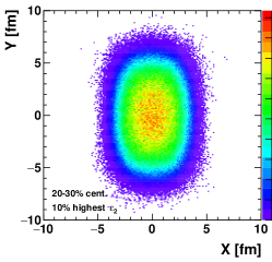
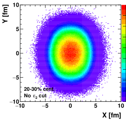
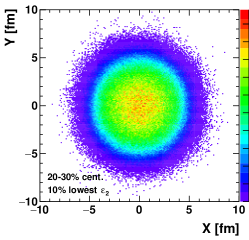
Figure 1 shows Glauber model calculations for 20-30% central Pb-Pb collisions at $\sqrt{s_{\rm NN}}=2.76\text{\,TeV}$ where in two cases a selection has been done on $\varepsilon_{2}$. As can be seen, this changes the geometry dramatically while keeping the “area” of the medium approximately fixed, which suggests that one does not change the average energy density of the QGP  but only the path length azimuthal asymmetry. By cutting on a variable related to the final measured integrated $v_{2}$ (the length of the 2nd-order flow vector) one can select (ESE) events with these extreme geometries. Importantly, these ideas have been tested and verified by experiments [7, 6].

By being able to vary the path length, $L$, while keeping the medium properties fixed, e.g. $\hat{q}$, one constrains the model significantly more than by $R_{\rm AA}$ and $v_{2}$ alone. I hope to convince the reader of this in the following.

A caveat of many measurements is that detectors have finite resolution and so selecting the top 10% $\varepsilon_{2}$ in data will not correspond to the top 10% in models. However, by comparing two ESE selections, $a$ and $b$, we can construct the ratio, $R_{\text{flow}}$:

$$R_{\text{flow}}\equiv\frac{\langle v_{2,a}(p_{\rm{T}})\rangle}{\langle v_{2,b}(p_{\rm{T}})\rangle}(p_{\rm{T}}<2\text{\,GeV/$c$})=\frac{k_{\text{flow}}(p_{\rm{T}})\langle\varepsilon_{2,a}\rangle}{k_{\text{flow}}(p_{\rm{T}})\langle\varepsilon_{2,b}\rangle}=\frac{\langle\varepsilon_{2,a}\rangle}{\langle\varepsilon_{2,b}\rangle},$$ (2)

which is, to first order, independent of $p_{\rm{T}}$ for hydrodynamic flow (i.e., for $p_{\rm{T}}<2\text{\,GeV/$c$}$). We note that this ratio gives us an experimental measure of the observed geometry variation that can be directly compared to geometry variations in model calculations, i.e., finite-resolution effects will make $R_{\text{flow}}$ closer to unity, but that can be mimicked in models by selecting broader $\varepsilon_{2}$ intervals. In Fig. 1, $R_{\text{flow}}=\,1.73$ (0.31) for the highest (lowest) $\varepsilon_{2}$ samples relative to the unbiased sample.

Now we turn to the high $p_{\rm{T}}$ region and the question of what we expect for the jet ratio

$$R_{\text{quench}}\equiv\frac{\langle v_{2,a}(p_{\rm{T}})\rangle}{\langle v_{2,b}(p_{\rm{T}})\rangle}(p_{\rm{T}}>10\text{\,GeV/$c$}).$$ (3)

If the jet quenching $v_{2}$ grows faster than the flow $v_{2}$ when increasing $\varepsilon_{2}$, then $R_{\text{quench}}>R_{\text{flow}}$ when we compare more asymmetric collisions to unbiased collisions, but $R_{\text{quench}}<R_{\text{flow}}$ when we compare more symmetric collisions to unbiased collisions.

The basic understanding of energy loss is that in different limits the path-length dependence can vary. If interference between adjacent interactions are important, as is expected for radiation energy loss, then the so-called Landau-Pomeranchuk-Migdal (LPM) effect will give a quadratic ($L^{2}$) pathlength dependence. However, if collisional energy loss plays a large role, or we are in the Bethe-Heitler (BH) limit where there is no interference, one expects a linear ($L$) dependence. Finally, in some strongly interacting QCD-like theories that can be solved via the Maldacena conjecture (the so called AdS-CFT correspondence) one finds a cubic ($L^{3}$) path-length dependence. In the following I will try to explain/justify that the jet-quenching $v_{2}$ can be approximately factorized like this:

$$v_{2}(p_{\rm{T}})\approx k_{\text{medium}}(p_{\rm{T}})k_{\text{pathlength}}(\varepsilon_{2}),$$ (4)

where $k_{\text{medium}}(p_{\rm{T}})$ encodes the strength of the coupling to the medium and $k_{\text{pathlength}}(\varepsilon_{2})$ encodes the path-length dependence. If we have a light quark and a gluon propagating through the medium then the gluon will in most models couple stronger to the QGP than the quark but the path-length dependence of the energy loss will be the same. Even the energy loss of gluons is therefore larger, the idea here is that, the relative variation of the energy loss (and therefore to some approximation $R_{\rm AA}$ and $v_{2}$) when doing the ESE is the same. For light and heavy quarks the color factor is the same but there can be kinematic differences at a fixed $p_{\rm{T}}$ due to the deadcone effect on the radiative energy loss of heavy quarks and the quark-mass difference for collisional and radiative energy loss. An example of the resulting energy-loss differences for light and heavy quarks can be found in Fig. 2 in [8]. But as long as this does not change the path-length dependence then one would again expect the relative changes to be the same. However, the factorization will break down if the path-length dependence varies with $p_{\rm{T}}$ (or in a more positive formulation, one can test this factorization with experimental data).

If Eq. 4 is a good approximation then:

$$R_{\text{quench}}\approx\frac{k_{\text{pathlength}}(\langle\varepsilon_{2,a}\rangle)}{k_{\text{pathlength}}(\langle\varepsilon_{2,b}\rangle)},$$ (5)

where we expect that $k_{\text{pathlength}}(\varepsilon_{2})$ is a monotonically increasing function of $\varepsilon_{2}$.

The claim is therefore that by measuring the ratio of $v_{2}(p_{\rm{T}})$ at low and high $p_{\rm{T}}$ for two ESE classes and taking their ratio one can get rid of the complicated functions $k_{\text{flow}}(p_{\rm{T}})$ and $k_{\text{medium}}(p_{\rm{T}})$ to narrow down the path-length dependence, $k_{\text{pathlength}}(\varepsilon_{2})$.

3 Estimating the ratio $R_{\text{quench}}$-to-$R_{\text{flow}}$ in a simple model

In [4], a simple model that could describe $R_{\rm AA}$ and $v_{2}$ at high $p_{\rm{T}}$ was developed. The model describes high-$p_{\rm{T}}$ charged hadrons with $p_{\rm{T}}\approx 10\text{\,GeV/$c$}$ based on the following assumptions/simplifications:

• The initial geometry is obtained from a Glauber calculation. For each event the participating nucleons are centered at (0, 0) and rotated so that the 2nd-order symmetry plane $\Psi_{2}=0$, see e.g. Fig 1.

• Jets are assumed to propagate from (0, 0) and the path length, $L$, is calculated as the standard deviation of the source in the direction of propagation: $\sigma_{X}$ in plane and $\sigma_{Y}$ out-of-plane.

• The source is assumed to be static and to have a uniform density of

  $$\rho=k\frac{{\rm d}N/{\rm d}\eta}{4\pi\sigma_{X}\sigma_{Y}},$$ (6)

  where $k$ is an unspecified constant, and $4\pi\sigma_{X}\sigma_{Y}$ is an estimate for the area of the medium.

• Only jets propagating in-plane and out-of-plane are considered.

The underlying idea is, just as in the previous section, that jet quenching depends mainly on two effects: medium density, $\rho$, and path length, $L$.

The $R_{\rm AA}$ and $v_{2}$ can be combined to estimate the $R_{\rm AA}$ in and out-of plane:

$$R_{\rm AA,in}(p_{\rm{T}}) \approx (1+2v_{2}(p_{\rm{T}}))R_{\rm AA}(p_{\rm{T}})$$ (7)

$$R_{\rm AA,out}(p_{\rm{T}}) \approx (1-2v_{2}(p_{\rm{T}}))R_{\rm AA}(p_{\rm{T}}),$$ (8)

using results from ALICE [9] and ATLAS [10]. The first step was to attempt to find a scaling variable $\rho^{a}L^{b}$ so that all the $R_{\rm AA,in}$ and $R_{\rm AA,out}$ would follow the same curve. At first, we were unsure if this was possible because one could expect that $L$ is not a good variable for the energy loss in plane where the source is expected to expand. We found that this was possible and took this as an indication that there is little or no effect on the effective path length of the transverse expansion, i.e., the path lengths evaluated for the initial state are meaningful variables for describing jet quenching.

A second issue turned out to be that, once a scaling variable is found the same scaling variable to any power also works. To find a unique solution, we demanded that the energy loss is roughly linear in this scaling variable. The $p_{\rm{T}}$ loss has been estimated in several PHENIX publications, e.g. [11], assuming that the difference between the expected and observed $p_{\rm{T}}$ spectra is mainly due to a $p_{\rm{T}}$ shift (loss). If one can parameterize the pp spectrum $dN/dp_{\rm{T}}$ by a power law, $k_{1}p_{\rm{T}}^{k_{2}}$, in the relevant $p_{\rm{T}}$ range, then one obtains a simple expression for the $p_{\rm{T}}$ loss:

$$\Delta p_{\rm{T}}=p_{\rm T,0}-p_{\rm T,final}=\left(1-R_{\rm AA}^{-1/(k_{2}+1)}\right)p_{\rm T,0},$$ (9)

where $p_{\rm T,0}$ is the initial $p_{\rm{T}}$. This non-linear relation between energy loss and $R_{\rm AA}$ complicates the intuitive understanding of how the function $k_{\text{pathlength}}(\varepsilon_{2})$ should behave because increasing the energy loss dramatically will eventually lead to much smaller changes in $R_{\rm AA}$.

In the estimate used here we take into account that quenching not only shifts but also compresses the spectrum.

Figure 2: Left: the $p_{\rm{T}}$ loss is found to scale with $\sqrt{\rho}L$ in exactly the same way at $\sqrt{s_{\rm NN}}=2.76\text{\,TeV}$ (PbPb), where the scaling relation was derived, and at $\sqrt{s_{\rm NN}}=200\text{\,GeV}$ (AuAu, data taken from [12]). The solid line is a linear fit. The dashed line is a fit that takes into account the decreasing $p_{\rm{T}}$ of the propagating particle leading to a small non-linear correction for large $p_{\rm{T}}$ losses. Right: the $p_{\rm{T}}$ losses corresponding to the initial geometries in Fig. 1 (when the small medium density variation is neglected).

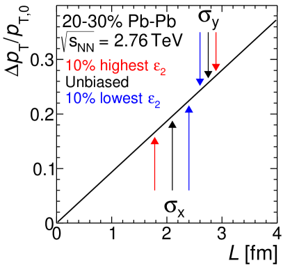
Figure 2 left shows the main result of [4]. The found scaling relation raises numerous questions that are beyond the scope of this proceeding. Here, I just want to point out that for symmetric systems, where $L_{\rm in}\approx L_{\rm out}$, the scaling variable is independent of $L$, $\Delta p_{\rm{T}}\propto\sqrt{{\rm d}N/{\rm d}\eta}$. A similar scaling was recently found by PHENIX [13]. Interestingly, if this result can be trusted, this would suggest that small systems produced in pp and p–Pb collisions should also exhibit jet quenching.

The main point of the scaling relation for this proceding is that, once you have such a model then you can further test it by fixing the medium properties ($\rho$) and varying the path length according to Fig. 1. Figure 2 right shows the predicted $p_{\rm{T}}$ loss from this model. To obtain $R_{\text{quench}}$ one simply estimates $R_{\rm AA,in}$ and $R_{\rm AA,out}$ using Eq. 9 and then determines $v_{2}$ from Eq. 7 and 8. For the concrete model, taking into account that $\rho$ changes slightly when we vary $\varepsilon_{2}$, we find:

$$10\%~{}\text{highest}~{}\varepsilon_{2}: R_{\text{quench}}\approx 1.05R_{\text{flow}}$$ (10)

$$10\%~{}\text{lowest}~{}\varepsilon_{2}: R_{\text{quench}}\approx 0.97R_{\text{flow}}$$ (11)

This means that jet quenching and flow have similar sensitivity to the azimuthal asymmetry of the initial overlap region.

ATLAS has measured $v_{2}$ as a function of $p_{\rm{T}}$ up to $15\text{\,GeV/$c$}$ for different ESE classes [10]. Within the large statistical uncertainties the ratio is flat (Fig. 3 top left in the paper), but for a definitive answer one will need the higher statistics of Run 2.

Note that recently similar calculations, as have been outlined in this section, have been done in a realistic model [14].

4 Conclusions and outlook

The $R_{\rm AA,in}$ and $R_{\rm AA,out}$ have proven to be difficult observables to describe for jet-quenching models. By doing these measurements as a function of the eccentricity one constrains the underlying geometry in a way that simplifies the direct interpretation of the results and that allows further tests of models.

Still, one does not avoid the need of a model to interpret the data. To be able to avoid models one would need two different probes. If one would measure $R_{\text{quench}}$ for light and heavy quarks then one could in principle compare these directly to understand if the effective path-length dependence of the energy loss is different, as expected from theoretical models. There is no reason to expect that the jet quenching $v_{2}$ of light and heavy quarks are the same because the coupling to the medium, $k_{\text{medium}}(p_{\rm{T}})$, can be different, but if the path-length dependence, $k_{\text{pathlength}}(p_{\rm{T}})$, is the same then one would to first order expect that $R_{\text{quench}}$ is the same (due to the non-linearity of energy loss and $R_{\rm AA}$, small differences can be expected) and so one can in a model independent way test if the path-length dependence, which is directly related to the physics mechanism of the energy loss, is the same or not.

The author would like to thank the organizers for a wonderful conference, Vytautas Vislavicius for making the additional Glauber-model calculations for these studies, and Jamie Nagle for comments to the proceeding.

References

- [1] PHENIX Collaboration, A. Adare et al., “Azimuthal anisotropy of neutral pion production in Au+Au collisions at = 200 GeV: Path-length dependence of jet quenching and the role of initial geometry,” Phys. Rev. Lett. 105 (2010) 142301, arXiv:1006.3740 [nucl-ex].
- [2] B. Betz and M. Gyulassy, “Examining a reduced jet-medium coupling in Pb+Pb collisions at the Large Hadron Collider,” Phys. Rev. C 86 (2012) 024903, arXiv:1201.0281 [nucl-th].
- [3] B. Betz and M. Gyulassy, “Constraints on the Path-Length Dependence of Jet Quenching in Nuclear Collisions at RHIC and LHC,” JHEP 08 (2014) 090, arXiv:1404.6378 [hep-ph]. [Erratum: JHEP10,043(2014)].
- [4] P. Christiansen, K. Tywoniuk, and V. Vislavicius, “Universal scaling dependence of QCD energy loss from data driven studies,” Phys. Rev. C 89 (2014) 034912, arXiv:1311.1173 [hep-ph].
- [5] J. Schukraft, A. Timmins, and S. A. Voloshin, “Ultra-relativistic nuclear collisions: event shape engineering,” Phys. Lett. B 719 (2013) 394–398, arXiv:1208.4563 [nucl-ex].
- [6] ALICE Collaboration, J. Adam et al., “Event shape engineering for inclusive spectra and elliptic flow in Pb-Pb collisions at TeV,” Phys. Rev. C 93 (2016) 034916, arXiv:1507.06194 [nucl-ex].
- [7] ATLAS Collaboration, G. Aad et al., “Measurement of the correlation between flow harmonics of different order in lead-lead collisions at =2.76 TeV with the ATLAS detector,” Phys. Rev. C 92 (2015) 034903, arXiv:1504.01289 [hep-ex].
- [8] S. Wicks, W. Horowitz, M. Djordjevic, and M. Gyulassy, “Elastic, inelastic, and path length fluctuations in jet tomography,” Nucl. Phys. A784 (2007) 426–442, arXiv:nucl-th/0512076 [nucl-th].
- [9] ALICE Collaboration, B. Abelev et al., “Centrality Dependence of Charged Particle Production at Large Transverse Momentum in Pb–Pb Collisions at TeV,” Phys. Lett. B 720 (2013) 52–62, arXiv:1208.2711 [hep-ex].
- [10] ATLAS Collaboration, G. Aad et al., “Measurement of the pseudorapidity and transverse momentum dependence of the elliptic flow of charged particles in lead-lead collisions at TeV with the ATLAS detector,” Phys. Lett. B 707 (2012) 330–348, arXiv:1108.6018 [hep-ex].
- [11] PHENIX Collaboration, S. S. Adler et al., “A Detailed Study of High-p(T) Neutral Pion Suppression and Azimuthal Anisotropy in Au+Au Collisions at s(NN)**(1/2) = 200-GeV,” Phys. Rev. C 76 (2007) 034904, arXiv:nucl-ex/0611007 [nucl-ex].
- [12] PHENIX Collaboration, A. Adare et al., “Neutral pion production with respect to centrality and reaction plane in AuAu collisions at =200 GeV,” Phys. Rev. C 87 (2013) 034911, arXiv:1208.2254 [nucl-ex].
- [13] PHENIX Collaboration, A. Adare et al., “Scaling properties of fractional momentum loss of high- hadrons in nucleus-nucleus collisions at from 62.4 GeV to 2.76 TeV,” Phys. Rev. C93 (2016) 024911, arXiv:1509.06735 [nucl-ex].
- [14] J. Noronha-Hostler, B. Betz, J. Noronha, and M. Gyulassy, “Soft-Hard Event Engineering in Ultrarelativistic Heavy Ion Collisions,” arXiv:1602.03788 [nucl-th].