Differentiability of a two-parameter family of self-affine functions

Abstract

This paper highlights an unexpected connection between expansions of real numbers to noninteger bases (so-called $\beta$-expansions) and the infinite derivatives of a class of self-affine functions. Precisely, we extend Okamoto’s function (itself a generalization of the well-known functions of Perkins and Katsuura) to a two-parameter family $\{F_{N,a}:N\in\mathbb{N},a\in(0,1)\}$. We first show that for each $x$, $F_{N,a}^{\prime}(x)$ is either $0$, $\pm\infty$, or undefined. We then extend Okamoto’s theorem by proving that for each $N$, depending on the value of $a$ relative to a pair of thresholds, the set $\{x:F_{N,a}^{\prime}(x)=0\}$ is either empty, uncountable but Lebesgue null, or of full Lebesgue measure. We compute its Hausdorff dimension in the second case.

The second result is a characterization of the set $\mathcal{D}_{\infty}(a):=\{x:F_{N,a}^{\prime}(x)=\pm\infty\}$, which enables us to closely relate this set to the set of points which have a unique expansion in the (typically noninteger) base $\beta=1/a$. Recent advances in the theory of $\beta$-expansions are then used to determine the cardinality and Hausdorff dimension of $\mathcal{D}_{\infty}(a)$, which depends qualitatively on the value of $a$ relative to a second pair of thresholds.

AMS 2010 subject classification: 26A27 (primary); 28A78, 11A63 (secondary)

Key words and phrases: Continuous nowhere differentiable function; infinite derivative; beta-expansion; Hausdorff dimension; Komornik-Loreti constant; Thue-Morse sequence.

1 Introduction

The aim of this paper is to investigate the differentiability of a two-parameter family of self-affine functions, constructed as follows. Fix a positive integer $N$ and a real parameter $a$ satisfying $1/(N+1)<a<1$, and let $b$ be the number such that $(N+1)a-Nb=1$. Note that $0<b<a$. Let $x_{i}:=i/(2N+1)$, $i=0,1,\dots,2N+1$, and for $j=0,1,\dots,N$, put $y_{2j}:=j(a-b)$, and $y_{2j+1}:=(j+1)a-jb$. Now set $f_{0}(x):=x$, and for $n=1,2,\dots$, define $f_{n}$ recursively on each interval $[x_{i},x_{i+1}]$ ($i=0,1,\dots,2N$) by

$$f_{n}(x):=y_{i}+(y_{i+1}-y_{i})f_{n-1}\big{(}(2N+1)(x-x_{i})\big{)},\qquad x_{i}\leq x\leq x_{i+1}.$$ (1)

Each $f_{n}$ is a continuous, piecewise linear function from the interval $[0,1]$ onto itself, and it is easy to see that the sequence $(f_{n})$ converges uniformly to a limit function which we denote by $F_{N,a}$. This function $F_{N,a}$ is again continuous and maps $[0,1]$ onto itself. It may be viewed as the self-affine function “generated” by the piecewise linear function with interpolation points $(x_{i},y_{i})$, $i=0,1,\dots,2N+1$. When $N=1$ we have Okamoto’s family of self-affine functions [22], which includes Perkins’ function [24] for $a=5/6$ and the Katsuura function [14] for $a=2/3$; see also Bourbaki [4]. Figure 1 illustrates the above construction for $N=1$; graphs of $F_{1,a}$ for two values of $a$ are shown in Figure 2; and Figure 3 illustrates the case $N=2$.

Figure 1: The first two steps in the construction of $F_{1,a}$

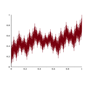
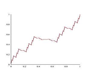
Figure 2: Graph of $F_{1,a}$ for $a=5/6$ (Perkins’ function; left) and $a=\hat{a}_{\infty}\doteq.5598$ (right).

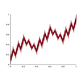
Figure 3: The generating pattern and graph of $F_{2,a}$, shown here for $a=0.6$.

The restriction $a>1/(N+1)$ is not necessary; when $a=1/(N+1)$ we have $b=0$ and $F_{N,a}$ is a generalized Cantor function. When $0<a<1/(N+1)$, we have $b<0$ and $F_{N,a}$ is strictly singular. Since the differentiability of such functions has been well-studied (e.g. [6, 7, 8, 10, 12, 15, 26]), we will focus exclusively on the case $a>1/(N+1)$, when $F_{N,a}$ is of unbounded variation. However, see [1] for a detailed analysis of the case $N=1$, $a\leq 1/2$.

Our main goal is to study the finite and infinite derivatives of $F_{N,a}$, thereby extending results of Okamoto [22] and Allaart [1]. We first show that for each $N$ the differentiability of $F_{N,a}$ follows the trichotomy discovered by Okamoto [22] for the case $N=1$: There are thresholds $\tilde{a}_{0}$ and $a_{0}^{*}$ (depending on $N$) such that $F_{N,a}$ is nowhere differentiable for $a\geq a_{0}^{*}$; nondifferentiable almost everywhere for $\tilde{a}_{0}\leq a<a_{0}^{*}$; and differentiable almost everywhere for $a<\tilde{a}_{0}$. We moreover compute the Hausdorff dimension of the exceptional sets implicit in the above statement.

In [1] a surprising connection was found between the infinite derivatives of $F_{1,a}$ and expansions of real numbers in noninteger bases. Our aim here is to generalize this result. We first give an explicit description of the set $\mathcal{D}_{\infty}(a)$ of points $x$ for which $F_{N,a}^{\prime}(x)=\pm\infty$, and then show that this set is closely related to the set $\mathcal{A}_{\beta}$ of real numbers which have a unique expansion in base $\beta$ over the alphabet $\{0,1,\dots,N\}$, where $\beta=1/a$. This allows us to express the Hausdorff dimension of $\mathcal{D}_{\infty}(a)$ directly in terms of the dimension of $\mathcal{A}_{\beta}$, which is known to vary continuously with $\beta$ and can be calculated explicitly for many values of $\beta$; see [17, 20]. We also take advantage of other recent breakthroughs in the theory of $\beta$-expansions to obtain a complete classification of the cardinality of $\mathcal{D}_{\infty}(a)$.

To end this introduction, we point out that the box-counting dimension of the graph of $F_{N,a}$ is given by

$$\dim_{B}\operatorname{Graph}(F_{N,a})=1+\frac{\log\big{(}2(N+1)a-1\big{)}}{\log(2N+1)},\qquad\frac{1}{N+1}<a<1.$$

This follows easily from the self-affine structure of $F_{N,a}$, for instance by using Example 11.4 of Falconer [9]. The Hausdorff dimension, on the other hand, does not appear to be known for any value of $a>1/(N+1)$, even when $N=1$; see the remark in the introduction of [1].

2 Main results

2.1 Finite derivatives

Following standard convention, we consider a function $f$ to be differentiable at a point $x$ if $f$ has a well-defined finite derivative at $x$. For each $N\in\mathbb{N}$, let $a_{\min}:=a_{\min}(N):=1/(N+1)$, let

$$a_{0}^{*}:=a_{0}^{*}(N):=\frac{3N+1}{(N+1)(2N+1)},$$ (2)

and let $\tilde{a}_{0}:=\tilde{a}_{0}(N)$ be the unique root in $(a_{\min},1)$ of the polynomial equation

$$(2N+1)^{2N+1}a^{N+1}\big{(}(N+1)a-1\big{)}^{N}=N^{N}.$$ (3)

The first ten values of $\tilde{a}_{0}(N)$ are shown in Table 1 below. Asymptotically, $\tilde{a}_{0}(N)\sim(1+\sqrt{2})/2N$ as $N\to\infty$; see Proposition 2.7 below.

The case $N=1$ of the following theorem is due to Okamoto [22], with the exception of the boundary value $a=\tilde{a}_{0}$, which was addressed by Kobayashi [16].

Theorem 2.1.

1. If $a_{0}^{*}\leq a<1$, then $F_{N,a}$ is nowhere differentiable;

2. If $\tilde{a}_{0}\leq a<a_{0}^{*}$, then $F_{N,a}$ is nondifferentiable almost everywhere, but is differentiable at uncountably many points;

3. If $a_{\min}<a<\tilde{a}_{0}$, then $F_{N,a}$ is differentiable almost everywhere, but is nondifferentiable at uncountably many points.

Moreover, if $F_{N,a}$ is differentiable at a point $x\in(0,1)$, then $F_{N,a}^{\prime}(x)=0$.

Statements (ii) and (iii) of the above theorem involve uncountably large sets of Lebesgue measure zero; it is of interest to determine their Hausdorff dimension. Let

$$\mathcal{D}_{0}(a):=\mathcal{D}_{0}^{(N)}(a):=\{x\in(0,1):F_{N,a}^{\prime}(x)=0\}.$$

Define the functions

$$\phi_{N}(a):=\frac{\log\big{(}(2N+1)a\big{)}}{\log(Na)-\log\big{(}(N+1)a-1\big{)}},\qquad a_{\min}<a<1,$$

and

$$h_{N}(p):=-\frac{1}{\log(2N+1)}\left[p\log\left(\frac{p}{N}\right)+(1-p)\log\left(\frac{1-p}{N+1}\right)\right],\qquad 0<p<1.$$

For a set $E\subset\mathbb{R}$, we denote the Hausdorff dimension of $E$ by $\dim_{H}E$.

Theorem 2.2.

1. If $\tilde{a}_{0}\leq a<a_{0}^{*}$, then $\dim_{H}\mathcal{D}_{0}^{(N)}(a)=h_{N}(\phi_{N}(a))$;

2. If $a_{\min}<a\leq\tilde{a}_{0}$, then $\dim_{H}\big{(}(0,1)\backslash\mathcal{D}_{0}^{(N)}(a)\big{)}=h_{N}(\phi_{N}(a))$;

3. The function $a\mapsto h_{N}(\phi_{N}(a))$ is concave on $a_{\min}<a<a_{0}^{*}$, takes on its maximum value of $1$ at $a=\tilde{a}_{0}$, and its limits as $a\downarrow a_{\min}$ and as $a\uparrow a_{0}^{*}$ are $\log(N+1)/\log(2N+1)$ and $\log N/\log(2N+1)$, respectively.

Observe that for $N\geq 2$, $\dim_{H}\mathcal{D}_{0}(a)$ has a discontinuity at $a_{0}^{*}$, where it jumps from $\log N/\log(2N+1)>0$ to $0$; see Figure 4.

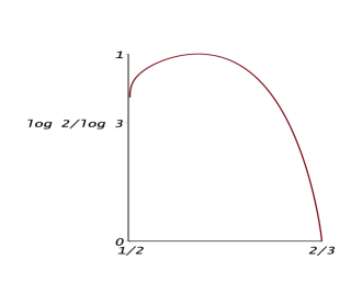
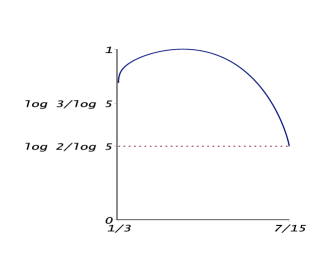
Figure 4: Graph of the function $h_{N}(\phi_{N}(a))$ from Theorem 2.2 for $N=1$ (left) and $N=2$ (right). While not clearly visible, the limits at the left endpoints are $\log 2/\log 3$ and $\log 3/\log 5$, respectively.

$$\begin{array}[]{r||c|c|c|c|c}N&a_{\min}(N)&\tilde{a}_{0}(N)&a_{0}^{*}(N)&\hat{a}_{\infty}(N)&a_{\infty}^{*}(N)\\ \hline\cr 1&\frac{1}{2}=.5000&.5592&\frac{2}{3}\approx.6667&.5598&.6180\\ 2&\frac{1}{3}\approx.3333&.3835&\frac{7}{15}\approx.4667&.4047&\frac{1}{2}=.5000\\ 3&\frac{1}{4}=.2500&.2914&\frac{5}{14}\approx.3571&.3444&.3660\\ 4&\frac{1}{5}=.2000&.2349&\frac{13}{45}\approx.2889&.2728&\frac{1}{3}\approx.3333\\ 5&\frac{1}{6}\approx.1667&.1967&\frac{8}{33}\approx.2424&.2534&.2638\\ 6&\frac{1}{7}\approx.1429&.1692&\frac{19}{91}\approx.2088&.2104&\frac{1}{4}=.2500\\ 7&\frac{1}{8}=.1250&.1484&\frac{11}{60}\approx.1833&.2014&.2071\\ 8&\frac{1}{9}\approx.1111&.1321&\frac{25}{153}\approx.1634&.1724&\frac{1}{5}=.2000\\ 9&\frac{1}{10}=.1000&.1191&\frac{14}{95}\approx.1474&.1674&.1708\\ 10&\frac{1}{11}\approx.0909&.1084&\frac{31}{231}\approx.1342&.1463&\frac{1}{6}\approx.1667\\ \hline\cr\end{array}$$

Table 1: Five important thresholds for $a$ determining differentiability of $F_{N,a}$

2.2 Infinite derivatives

For $x\in[0,1)$, let

$$x=0.\xi_{1}\xi_{2}\xi_{3}\cdots=\sum_{i=1}^{\infty}\xi_{i}(2N+1)^{-i}$$

denote the expansion of $x$ in base $2N+1$, so $\xi_{i}\in\{0,1,\dots,2N\}$ for each $i$. When $x$ has two such expansions, we take the one ending in all zeros. Let

$$M(x):=\#\{i\in\mathbb{N}:\xi_{i}\ \mbox{is odd}\}.$$

We also write $\omega_{i}:=\xi_{i}/2$, and note that when $\xi_{i}$ is even, $\omega_{i}\in A:=\{0,1,\dots,N\}$. For $d\in A$, write $\bar{d}:=N-d$.

Theorem 2.3.

Let $a_{\min}<a<1$. A point $x\in(0,1)$ satisfies $F_{N,a}^{\prime}(x)=\pm\infty$ if and only if $M(x)<\infty$ and the following two limits hold:

$$\lim_{n\to\infty}\big{(}(2N+1)a\big{)}^{n}\left(1-\sum_{j=1}^{\infty}a^{j}\omega_{n+j}\right)=\infty,$$ (4)

and

$$\lim_{n\to\infty}\big{(}(2N+1)a\big{)}^{n}\left(1-\sum_{j=1}^{\infty}a^{j}\overline{\omega_{n+j}}\right)=\infty.$$ (5)

Assuming all these conditions are satisfied, $F_{N,a}^{\prime}(x)=\infty$ if $M(x)$ is even, and $F_{N,a}^{\prime}(x)=-\infty$ if $M(x)$ is odd.

While the conditions (4) and (5) may look complicated at first sight, readers familiar with $\beta$-expansions will recognize the summations appearing in them. For a real number $1<\beta<N+1$ and $x\in\mathbb{R}$, we call an expression of the form

$$x=\sum_{j=1}^{\infty}\frac{\omega_{j}}{\beta^{j}},\qquad\mbox{where $\omega_{1},\omega_{2},\dots\in A$}$$ (6)

an expansion of $x$ in base $\beta$ over the alphabet $A$ (or simply, a $\beta$-expansion). Clearly such an expansion exists if and only if $0\leq x\leq N/(\beta-1)$. It is well known (see [25]) that almost every $x$ in this interval has a continuum of $\beta$-expansions. For the purpose of this article, we reduce the interval a bit further and consider the so-called univoque set

$$\mathcal{A}_{\beta}:=\{x\in((N-\beta+1)/(\beta-1),1):x\ \mbox{has a {\em unique} expansion of the form \eqref{eq:beta-expansion}}\}.$$

Let $\Omega:=A^{\mathbb{N}}$. For $\beta>1$, let $\Pi_{\beta}:\Omega\to\mathbb{R}$ denote the projection map given by

$$\Pi_{\beta}(\omega)=\sum_{j=1}^{\infty}\frac{\omega_{j}}{\beta^{j}},\qquad\omega=\omega_{1}\omega_{2}\cdots\in\Omega,$$

so that (6) can be written compactly as $x=\Pi_{\beta}(\omega)$. Let $\sigma$ denote the left shift map on $\Omega$; that is, $\sigma(\omega_{1}\omega_{2}\cdots)=\omega_{2}\omega_{3}\cdots$. Define the set

$$\mathcal{U}_{\beta}:=\Pi_{\beta}^{-1}(\mathcal{A}_{\beta}).$$

It is essentially due to Parry [23] (see also [1, Lemma 5.1]) that

$$\omega\in\mathcal{U}_{\beta}\qquad\Longleftrightarrow\qquad\Pi_{\beta}(\sigma^{n}(\omega))<1\ \mbox{and}\ \Pi_{\beta}(\sigma^{n}(\bar{\omega}))<1\ \mbox{for all $n\geq 0$},$$

and this, together with Theorem 2.3, suggests a close connection between the set

$$\mathcal{D}_{\infty}(a):=\mathcal{D}_{\infty}^{(N)}(a):=\{x\in(0,1):F_{N,a}^{\prime}(x)=\pm\infty\}$$

and the univoque set $\mathcal{A}_{\beta}$, where $\beta=1/a$. The size of $\mathcal{A}_{\beta}$ has been well-studied, starting with the remarkable theorem of Glendinning and Sidorov [11]. There are two pertinent thresholds, which we now define. First, for $N\in\mathbb{N}$, let

$$G(N):=\begin{cases}m+1&\mbox{if $N=2m$},\\ \frac{m+\sqrt{m^{2}+4m}}{2}&\mbox{if $N=2m-1$}.\end{cases}$$

Baker [3] calls $G(N)$ a generalized golden ratio, because $G(1)=(1+\sqrt{5})/2$.

Next, recall that the Thue-Morse sequence is the sequence $(\tau_{j})_{j=0}^{\infty}$ of $0$’s and $1$’s given by $\tau_{j}=s_{j}\operatorname{mod}2$, where $s_{j}$ is the number of $1$’s in the binary representation of $j$. Thus,

$$(\tau_{j})_{j=0}^{\infty}=0110\ 1001\ 1001\ 0110\ 1001\ 0110\ 0110\ 1001\ \dots$$

For each $N\in\mathbb{N}$, define a generalized Thue-Morse sequence $\tau^{(N)}=\big{(}\tau_{i}^{(N)}\big{)}_{i=1}^{\infty}$ by

$$\tau_{i}^{(N)}:=\begin{cases}m-1+\tau_{i}&\mbox{if $N=2m-1$},\\ m+\tau_{i}-\tau_{i-1}&\mbox{if $N=2m$}.\end{cases}$$

Finally, let $\beta_{c}:=\beta_{c}(N)$ be the Komornik-Loreti constant [18, 19]; that is, $\beta_{c}$ is the unique positive value of $\beta$ such that

$$\Pi_{\beta}\left(\tau^{(N)}\right)=1.$$

The following theorem is due to Glendinning and Sidorov [11] for $N=1$, and to Kong et al. [21] and Baker [3] for $N\geq 2$.

Theorem 2.4.

The set $\mathcal{A}_{\beta}$ is:

1. empty if $\beta\leq G(N)$;

2. nonempty but countable if $G(N)<\beta<\beta_{c}(N)$;

3. uncountable but of Hausdorff dimension zero if $\beta=\beta_{c}(N)$;

4. of positive Hausdorff dimension if $\beta>\beta_{c}(N)$.

(In case (ii), there is a further threshold between $G(N)$ and $\beta_{c}(N)$ that separates finite and infinite cardinalities of $\mathcal{A}_{\beta}$, but this is not relevant to our present aims.)

Now let $a_{\infty}^{*}:=a_{\infty}^{*}(N):=1/G(N)$, and $\hat{a}_{\infty}:=\hat{a}_{\infty}(N):=1/\beta_{c}(N)$. For a finite set $S$, let $S^{*}$ denote the set of all finite sequences of elements of $S$, including the empty sequence.

Theorem 2.5.

1. For all $a\in(\hat{a}_{\infty},1)$ and for almost all $a\in(a_{\min},\hat{a}_{\infty})$,

   $$\mathcal{D}_{\infty}(a)=\left\{\Pi_{2N+1}(v\cdot 2\omega):v\in\{0,1,\dots,2N\}^{*},\omega\in\mathcal{U}_{1/a}\right\},$$ (7)

   where $2\omega:=(2\omega_{1},2\omega_{2},\dots)$ and $v\cdot 2\omega$ denotes the concatenation of $v$ with $2\omega$;

2. For all $a\in(a_{\min},1)$, $\mathcal{D}_{\infty}(a)$ is a subset of the set in the right-hand-side of (7), and the inclusion is proper for infinitely many $a\in(a_{\min},\hat{a}_{\infty}]$, including $\hat{a}_{\infty}$ itself;

3. For all $a\in(a_{\min},1)$,

   $$\dim_{H}\mathcal{D}_{\infty}(a)=\frac{\log(1/a)}{\log(2N+1)}\dim_{H}\mathcal{A}_{1/a}.$$ (8)

Theorem 2.5(i) says that for almost all $a$, the set $\mathcal{D}_{\infty}(a)$ consists precisely of those points whose base $2N+1$ expansion is obtained by taking an arbitrary point $x$ having a unique expansion in base $\beta$ (where $\beta=1/a$), doubling the base $\beta$ digits of $x$, and appending the resulting sequence to an arbitrary finite prefix of digits from $\{0,1,\dots,2N\}$.

Corollary 2.6.

The set $\mathcal{D}_{\infty}(a)$ is:

1. empty if $a\geq a_{\infty}^{*}$;

2. countably infinite, containing only rational points, if $\hat{a}_{\infty}<a<a_{\infty}^{*}$;

3. uncountable with Hausdorff dimension zero if $a=\hat{a}_{\infty}$;

4. of strictly positive Hausdorff dimension if $a_{\min}<a<\hat{a}_{\infty}$.

Moreover, on the interval $(a_{\min},\hat{a}_{\infty})$, the function $a\mapsto\dim_{H}\mathcal{D}_{\infty}(a)$ is continuous and nonincreasing, and its points of decrease form a set of Lebesgue measure zero.

Regarding the relative ordering and the asymptotics of the five thresholds in Table 1, we have the following:

Proposition 2.7.

1. For each $N\geq 5$, we have

   $$a_{\min}(N)<\tilde{a}_{0}(N)<a_{0}^{*}(N)<\hat{a}_{\infty}(N)<a_{\infty}^{*}(N).$$ (9)

2. As $N\to\infty$, we have

   $$Na_{\min}(N)\to 1,\qquad N\tilde{a}_{0}(N)\to\frac{1+\sqrt{2}}{2}=1.207\cdots,$$

   $$Na_{0}^{*}(N)\to\frac{3}{2},\qquad N\hat{a}_{\infty}(N)\to 2,\qquad Na_{\infty}^{*}(N)\to 2.$$

It is interesting to observe that for $N=1$, there is an interval of $a$-values (namely, $a_{\infty}^{*}<a<a_{0}^{*}$) for which $\dim_{H}\mathcal{D}_{0}(a)>0$ but $\mathcal{D}_{\infty}(a)=\emptyset$. In other words, for such $a$ there are uncountably many points where $F_{N,a}$ is differentiable, but no points where it has an infinite derivative. For $2\leq N\leq 4$ there is no such $a$, but there is still an interval (namely, $\hat{a}_{\infty}<a<a_{0}^{*}$) for which $\dim_{H}\mathcal{D}_{0}(a)>0$ but $\mathcal{D}_{\infty}(a)$ is only countable. For all $N\geq 5$, however, $\dim_{H}\mathcal{D}_{\infty}(a)>0$ whenever $\dim_{H}\mathcal{D}_{0}(a)>0$.

3 Proofs of Theorems 2.1 and 2.2

Recall that for $x\in[0,1)$, $x=0.\xi_{1}\xi_{2}\xi_{3}\cdots$ denotes the expansion of $x$ in base $2N+1$. We first introduce some additional notation. For $n\in\mathbb{N}$, let $i(n):=i(n;x)$ denote the number of odd digits among $\xi_{1},\dots,\xi_{n}$. Let $x_{n,j}:=j/(2N+1)^{n}$, and put $I_{n,j}:=[x_{n,j},x_{n,j+1})$ for $n\in\mathbb{N}\cup\{0\}$ and $j\in\mathbb{Z}$. For $x\in(0,1)$ and $n\in\mathbb{N}\cup\{0\}$, let $I_{n}(x)$ denote that interval $I_{n,j}$ which contains $x$.

The first important observation is that

$$F_{N,a}(x_{n,j})=f_{n}(x_{n,j}),\qquad\mbox{for $j=0,1,\dots,(2N+1)^{n}$}.$$ (10)

Next, recall that $b$ is the number such that $(N+1)a-Nb=1$. The recursive construction of the piecewise linear approximants $f_{n}$ implies that

$$f_{n}^{\prime}(x)=(2N+1)^{n}a^{n-i(n)}(-b)^{i(n)},$$ (11)

at all $x$ not of the form $x_{n,j}$, $j\in\mathbb{Z}$. As a result,

$$\frac{f_{n+1}^{\prime}(x)}{f_{n}^{\prime}(x)}\in\{(2N+1)a,-(2N+1)b\},$$

and since neither of these two values equals $1$, $f_{n}^{\prime}(x)$ cannot converge to a nonzero finite number. Clearly, if $F_{N,a}^{\prime}(x)$ exists, it must be equal to $\lim_{n\to\infty}f_{n}^{\prime}(x)$ in view of (10). The only possible finite value of $F_{N,a}^{\prime}(x)$, therefore, is zero.

Lemma 3.1.

For $x\in(0,1)$, $F_{N,a}^{\prime}(x)=0$ if and only if $\lim_{n\to\infty}f_{n}^{\prime}(x)=0$.

Proof.

Only the “if” part requires proof. For simplicity, write $F:=F_{N,a}$. Let $s_{n,j}$ denote the slope of $f_{n}$ on the interval $I_{n,j}$. An easy induction argument shows that

$$\frac{s_{n,j+1}}{s_{n,j}}\in\left\{-\frac{a}{b},-\frac{b}{a}\right\},\qquad j=0,1,\dots,(2N+1)^{n}-2.$$ (12)

Furthermore,

$$x\in I_{n,j}\quad\Rightarrow\quad\min\{F(x_{n,j}),F(x_{n,j+1})\}\leq F(x)\leq\max\{F(x_{n,j}),F(x_{n,j+1})\}.$$ (13)

Now assume $f_{n}^{\prime}(x)\to 0$. Fix $h>0$, let $n$ be the integer such that $(2N+1)^{-n-1}<h\leq(2N+1)^{-n}$, and let $j$ be such that $I_{n,j}=I_{n}(x)$. Then $x_{n,j}\leq x<x_{n,j+1}$ and $x_{n,j}\leq x+h<x_{n,j+2}$. If $x+h>x_{n,j+1}$, (13) gives

$$|F(x+h)-F(x)| \leq|F(x+h)-F(x_{n,j+1})|+|F(x_{n,j+1})-F(x)|$$

$$\leq|F(x_{n,j+2})-F(x_{n,j+1})|+|F(x_{n,j+1})-F(x_{n,j})|$$

$$=(2N+1)^{-n}\left(|s_{n,j+1}|+|s_{n,j}|\right)$$

$$\leq(1+C)(2N+1)^{-n}|s_{n,j}|$$

$$=(1+C)(2N+1)^{-n}|f_{n}^{\prime}(x)|,$$

where $C:=\max\{a/b,b/a\}$, and the last inequality follows from (12). If $x+h\leq x_{n,j+1}$, the same bound follows even more directly. Thus, we obtain the estimate

$$\left|\frac{F(x+h)-F(x)}{h}\right|\leq(2N+1)(1+C)|f_{n}^{\prime}(x)|,$$

showing that $F$ has a vanishing right derivative at $x$. By a similar argument, $F$ has a vanishing left derivative at $x$ as well, and hence, $F^{\prime}(x)=0$. ∎

Now define

$$l(x):=\liminf_{n\to\infty}\frac{i(n;x)}{n},\qquad x\in(0,1),$$

and use (11) to write

$$|f_{n}^{\prime}(x)|=\left[(2N+1)a\left(\frac{b}{a}\right)^{i(n)/n}\right]^{n}.$$

The significance of the function $\phi_{N}(a)$ is that

$$(2N+1)a\left(\frac{b}{a}\right)^{\phi_{N}(a)}=1.$$

Since $0<b/a<1$, this last equation together with Lemma 3.1 implies

$$\left\{x\in(0,1):l(x)>\phi_{N}(a)\right\}\subseteq\mathcal{D}_{0}(a)\subseteq\left\{x\in(0,1):l(x)\geq\phi_{N}(a)\right\}.$$ (14)

Proof of Theorem 2.1.

(i) Assume first that $a\geq a_{0}^{*}$. Since $a>b>0$, (11) yields

$$|f_{n}^{\prime}(x)|\geq\big{(}(2N+1)b\big{)}^{n}=\left[\frac{2N+1}{N}\big{(}(N+1)a-1\big{)}\right]^{n}\geq 1$$

for every $x$ not of the form $k/(2N+1)^{n}$, so $f_{n}^{\prime}(x)\not\to 0$ for such $x$. Hence, $F_{N,a}$ is nowhere differentiable.

(ii) and (iii): By Borel’s normal number theorem,

$$\lim_{n\to\infty}\frac{i(n;x)}{n}=\frac{N}{2N+1}\qquad\mbox{for almost every $x\in(0,1)$}.$$ (15)

By definition of $\tilde{a}_{0}$, we have $\phi_{N}(\tilde{a}_{0})=N/(2N+1)$. Moreover, $\phi_{N}$ is monotone increasing on $(a_{\min},a_{0}^{*})$. From these observations, it follows via (14) and (15) that $\mathcal{D}_{0}(a)$ has Lebesgue measure one if $a_{\min}<a<\tilde{a}_{0}$, and Lebesgue measure zero if $a>\tilde{a}_{0}$. Finally, the law of the iterated logarithm implies that for almost every $x\in(0,1)$, $i(n;x)/n<N/(2N+1)=\phi_{N}(\tilde{a}_{0})$, and therefore $|f_{n}^{\prime}(x)|\geq 1$, for infinitely many $n$. (See [16] for more details in the case $N=1$). Thus, $\mathcal{D}_{0}(\tilde{a}_{0})$ has measure zero as well. The remaining statements follow from Theorem 2.2, which is proved below. ∎

In view of the relations (14), we define for $p\in(0,1)$ the sets

$$R_{p}:=\{x\in(0,1):l(x)>p\},\qquad\bar{R}_{p}:=\{x\in(0,1):l(x)\geq p\},$$

$$S_{p}:=\{x\in(0,1):l(x)<p\},\qquad\bar{S}_{p}:=\{x\in(0,1):l(x)\leq p\}.$$

Lemma 3.2.

We have

$$\dim_{H}R_{p}=\dim_{H}\bar{R}_{p}=\begin{cases}1&\mbox{if $0<p\leq N/(2N+1)$},\\ h_{N}(p)&\mbox{if $N/(2N+1)\leq p<1$},\end{cases}$$ (16)

and

$$\dim_{H}S_{p}=\dim_{H}\bar{S}_{p}=\begin{cases}h_{N}(p)&\mbox{if $0<p\leq N/(2N+1)$},\\ 1&\mbox{if $N/(2N+1)\leq p<1$}.\end{cases}$$ (17)

Proof.

We prove (16); the proof of (17) is analogous. Since $\bar{R}_{p}\supseteq R_{p}\supseteq\bar{R}_{p-{\varepsilon}}$ for all $p>{\varepsilon}>0$ and $h_{N}$ is continuous in $p$, it suffices to compute $\dim_{H}\bar{R}_{p}$. First define, for nonnegative real numbers $p_{0},\dots,p_{2N}$ with $p_{0}+\dots+p_{2N}=1$, the set

$$\mathcal{F}(p_{0},\dots,p_{2N}):=\left\{x\in(0,1):\lim_{n\to\infty}\frac{\#\{j\leq n:\xi_{j}(x)=i\}}{n}=p_{i},\quad i=0,1,\dots,2N\right\}.$$

It is well known (see, for instance, [9, Proposition 10.1]) that

$$\dim_{H}\mathcal{F}(p_{0},\dots,p_{2N})=-\frac{1}{\log(2N+1)}{\sum_{i=0}^{2N}p_{i}\log p_{i}}.$$ (18)

If $0<p\leq N/(2N+1)$, then $\bar{R}_{p}$ has Lebesgue measure one by (15). Suppose $N/(2N+1)<p<1$. Then $\bar{R}_{p}$ contains the set

$$\mathcal{F}\left(\frac{1-p}{N+1},\frac{p}{N},\frac{1-p}{N+1},\dots,\frac{p}{N},\frac{1-p}{N+1}\right),$$

which has Hausdorff dimension $h_{N}(p)$ by (18). Therefore, $\dim_{H}\bar{R}_{p}\geq h_{N}(p)$.

For the reverse inequality, we introduce a probability measure $\mu$ on $(0,1)$ as follows. Set

$$\mu(I_{n}(x)):=\left(\frac{p}{N}\right)^{i(n;x)}\left(\frac{1-p}{N+1}\right)^{n-i(n;x)}.$$

This defines $\mu(I_{n,j})$ for all $n\in\mathbb{N}\cup\{0\}$ and $j=0,1,\dots,(2N+1)^{n}-1$ in such a way that $\mu(I_{n,j})=\sum_{\nu=0}^{2N}\mu(I_{n+1,(2N+1)j+\nu})$ for all $n$ and $j$, and hence $\mu$ extends uniquely to a Borel probability measure on $(0,1)$, which we again denote by $\mu$. It is a routine exercise that $\mu$ concentrates its mass on the set $\{x:\lim_{n\to\infty}i(n;x)/n=p\}$, so in particular $\mu(\bar{R}_{p})=1$. It now follows just as in the proof of [1, Lemma 4.2] that if $s>h_{N}(p)$, then

$$\limsup_{n\to\infty}\frac{\mu(I_{n}(x))}{|I_{n}(x)|^{s}}=\infty,$$

where $|I_{n}(x)|$ denotes the length of $I_{n}(x)$. Using [9, Proposition 4.9], we conclude that $\dim_{H}\bar{R}_{p}\leq h_{N}(p)$. ∎

Proof of Theorem 2.2.

Statements (i) and (ii) follow immediately from Lemma 3.2 and (14). The proof of (iii) is a straightforward calculus exercise. ∎

4 Proof of Theorem 2.3

To avoid notational clutter we again write $F:=F_{N,a}$. In order for $F$ to have an infinite derivative at $x$, it is clear that $f_{n}^{\prime}(x)$ must tend to $\pm\infty$. By (11), this is the case if and only if $\xi_{n}$ is even for all but finitely many $n$. However, it turns out that this condition is not sufficient.

We begin with an infinite-series representation of $F$ (see [16] for a proof when $N=1$):

$$F(x)=\sum_{n=1}^{\infty}a^{n-1-i(n-1)}(-b)^{i(n-1)}y_{\xi_{n}},$$

where $y_{0},y_{1},\dots,y_{2N}$ are the numbers used in the introduction to define $f_{n}$. In the special case when $\xi_{n}$ is even for every $n$, this reduces to

$$F(x)=\frac{1}{N}\sum_{n=1}^{\infty}a^{n-1}(1-a)\omega_{n},$$ (19)

where $\omega_{n}:=\xi_{n}/2$, and we have used that $i(a-b)=i(1-a)/N$ for $i=0,1,\dots,N$. Let $F_{+}^{\prime}$ and $F_{-}^{\prime}$ denote the right-hand and left-hand derivative of $F$, respectively.

Lemma 4.1.

Assume $\xi_{n}(x)$ is even for every $x$, and let $\omega_{n}:=\xi_{n}(x)/2$. Then $F_{+}^{\prime}(x)=\infty$ if and only if

$$\lim_{n\to\infty}\big{(}(2N+1)a\big{)}^{n}\left(1-\sum_{k=1}^{\infty}a^{k}\omega_{n+k}\right)=\infty.$$ (20)

Proof.

For each $n\in\mathbb{N}$, let $j_{n}$ be the integer such that $x\in I_{n,j_{n}}$, and put $z_{n}:=x_{n,j_{n}+2}$ (the right endpoint of $I_{n,j_{n}+1}$). In order that $F_{+}^{\prime}(x)=\infty$, it is clearly necessary that

$$\lim_{n\to\infty}\frac{F(z_{n})-F(x)}{z_{n}-x}=\infty.$$ (21)

The slope of $f_{n}$ on $I_{n,j_{n}}$ is $\big{(}(2N+1)a\big{)}^{n}$, and by (12), the slope of $f_{n}$ on $I_{n,j_{n}+1}$ is $-(2N+1)^{n}a^{n-1}b$, independent of $\xi_{n}$. Therefore, the difference $F(z_{n})-F(x)$ does not depend on $\xi_{n}$, and we may assume $\xi_{n}=0$. Then $z_{n}=0.\xi_{1}\xi_{2}\cdots\xi_{n-1}200\cdots$, and (19) applied to $x$ and $z_{n}$ (noting that $\omega_{n}(x)=0$ and $\omega_{n}(z_{n})=1$) gives

$$F(z_{n})-F(x) =a^{n-1}\frac{1-a}{N}-\sum_{k=n+1}^{\infty}a^{k-1}\frac{(1-a)\omega_{k}}{N}$$

$$=\frac{a^{n-1}(1-a)}{N}\left(1-\sum_{k=1}^{\infty}a^{k}\omega_{n+k}\right).$$

Since $1/(2N+1)^{n}<z_{n}-x\leq 2/(2N+1)^{n}$, it follows that (21) is equivalent to (20), showing that (20) is necessary. We now demonstrate that it is also sufficient.

Assume (20), or equivalently, (21). Then $F(z_{n})>F(x)$ for all large enough $n$. Given $h>0$, let $n\in\mathbb{N}$ such that $(2N+1)^{-n-1}<h\leq(2N+1)^{-n}$, let $j:=j_{n}$, and as before, $z_{n}:=x_{n,j+2}$. If $x+h\geq x_{n,j+1}$, then, since $f_{n}^{\prime}<0$ on $(x_{n,j+1},x_{n,j+2})$, we have by (13),

$$\frac{F(x+h)-F(x)}{h}\geq\frac{F(z_{n})-F(x)}{h}\geq\frac{F(z_{n})-F(x)}{z_{n}-x}\to\infty,$$

where the last inequality holds for all sufficiently large $n$.

Assume now that $x+h<x_{n,j+1}$. Then $\xi_{n+1}=2i$ for some $i<N$, so $x\in I_{n+1,(2N+1)j+2i}$ and $z_{n+1}=x_{n+1,(2N+1)j+2i+2}<x_{n,j+1}$. Moreover, $x_{n+1,(2N+1)j+2i+1}<x+h<z_{n,j+1}$. In view of (13) and the zig-zag pattern in the graph of $f_{n+1}$, it follows that $F(x+h)\geq F(z_{n+1})$. Finally, $h\leq(2N+1)(z_{n+1}-x)$. Combining these facts, we obtain, for all sufficiently large $n$,

$$\frac{F(x+h)-F(x)}{h}\geq\frac{F(z_{n+1})-F(x)}{h}\geq\frac{F(z_{n+1})-F(x)}{(2N+1)(z_{n+1}-x)}.$$

Thus, by (21), $F_{+}^{\prime}(x)=\infty$. ∎

Proof of Theorem 2.3.

If $x=j/(2N+1)^{n}$ for some $n\in\mathbb{N}$ and $j\in\mathbb{Z}$, then it follows immediately from (12) that $F_{+}^{\prime}(x)$ and $F_{-}^{\prime}(x)$ are of opposite signs (in fact, one $+\infty$, the other $-\infty$), so $F$ does not have an infinite derivative at $x$. And since $\omega_{n}=\xi_{n}=0$ for all but finitely many $n$ in this case,

$$\sum_{j=1}^{\infty}a^{j}\overline{\omega_{n+j}}=\sum_{j=1}^{\infty}a^{j}N=\frac{aN}{1-a}>1$$

for all sufficiently large $n$, so (5) fails.

Now assume that $x$ is not of the form $j/(2N+1)^{n}$, and let $m:=M(x)$. As already observed earlier, $F$ does not have an infinite derivative at $x$ if $m=\infty$, so assume $m<\infty$. Since $F(1-x)=1-F(x)$, it follows that $F_{-}^{\prime}(x)=F_{+}^{\prime}(1-x)$ when at least one of these two quantities exists, and moreover, $\xi_{n}(1-x)=2N-\xi_{n}(x)$ and so $\omega_{n}(1-x)=\overline{\omega_{n}(x)}$ when $\xi_{n}(x)$ is even. Therefore, it suffices to show that $F_{+}^{\prime}(x)=\pm\infty$ if and only if (4) holds. If $m=0$, this is immediate from Lemma 4.1, so assume $m>0$. Choose $n_{0}$ so that $\xi_{n}$ is even for all $n\geq n_{0}$, let $j$ be the integer such that $x\in I_{n_{0},j}=[x_{n_{0},j},x_{n_{0},j+1})$. Then $x=x_{n_{0},j}+(2N+1)^{-n_{0}}\hat{x}$, where $\hat{x}\in[0,1)$ satisfies the hypothesis of Lemma 4.1, and $M(x_{n_{0},j})=M(x)=m$. Note that (20) holds for $\hat{x}$ if and only if it holds for $x$, since the condition is invariant under a shift of the sequence $(\xi_{n})$. The graph of $F$ above $I_{n_{0},j}$ is an affine copy of the full graph of $F$, scaled horizontally by $(2N+1)^{-n_{0}}$ and vertically by $a^{n_{0}-m}b^{m}$, and reflected top-to-bottom if $m$ is odd. Thus, $F_{+}^{\prime}(x)$ is infinite if and only if $F_{+}^{\prime}(\hat{x})$ is, with the same sign when $m$ is even, and the opposite sign when $m$ is odd. ∎

5 Proofs of Theorem 2.5 and Corollary 2.6

Proof of Theorem 2.5.

We will need the auxiliary sets

$$\widetilde{\mathcal{U}}_{\beta}:=\{\omega\in\mathcal{U}_{\beta}:\limsup_{n\to\infty}\Pi_{\beta}(\sigma^{n}(\omega))<1\ \mbox{and}\ \limsup_{n\to\infty}\Pi_{\beta}(\sigma^{n}(\bar{\omega}))<1\},$$ (22)

for $1<\beta<N+1$, as well as the family of affine maps

$$\psi_{n,k}(x):=(2N+1)^{-n}(x+k),\qquad n\in\mathbb{N},\quad k=0,1,\dots,(2N+1)^{n}-1,$$

and the function $\Phi:\Omega\to[0,1]$ given by

$$\Phi(\omega):=2\Pi_{2N+1}(\omega),\qquad\omega\in\Omega.$$ (23)

Since $a>a_{\min}$ implies that $\big{(}(2N+1)a\big{)}^{n}\to\infty$, it follows from Theorem 2.3 that

$$\bigcup_{n,k}\psi_{n,k}\big{(}\Phi\big{(}\widetilde{\mathcal{U}}_{1/a}\big{)}\big{)}\subset\mathcal{D}_{\infty}(a)\subset\bigcup_{n,k}\psi_{n,k}(\Phi(\mathcal{U}_{1/a})),$$ (24)

where the unions are over $n\in\mathbb{N}$ and $k=0,1,\dots,(2N+1)^{n}-1$. Note that the set on the far right of (24) is precisely the set on the right hand side of (7). It was shown in [2] that $\widetilde{\mathcal{U}}_{\beta}=\mathcal{U}_{\beta}$ for all $1<\beta<\beta_{c}(N)$ and almost all $\beta_{c}(N)<\beta<N+1$, so (24) yields (i) and the first part of (ii). It was further shown in [2] that there are infinitely many values of $\beta$, including $\beta_{c}(N)$, for which $\widetilde{\mathcal{U}}_{\beta}$ is a proper subset of $\mathcal{U}_{\beta}$, and that for each such $\beta$ and any given sequence $(\theta_{n})$ of positive numbers, there are in fact uncountably many $\omega\in\mathcal{U}_{\beta}\backslash\widetilde{\mathcal{U}}_{\beta}$ such that

$$\liminf_{n\to\infty}\theta_{n}\big{(}1-\Pi_{\beta}(\sigma^{n}(\omega))\big{)}<\infty.$$

Taking $\theta_{n}=\big{(}(2N+1)a\big{)}^{n}$ we obtain the second part of statement (ii).

To prove (iii), we consider Hausdorff dimension in the sequence space $\Omega$. For each $\beta>1$, define a metric $\rho_{\beta}$ on $\Omega$ by $\rho_{\beta}(\omega,\eta):=\beta^{-\inf\{i:\omega_{i}\neq\eta_{i}\}}$ for $\omega=\omega_{1}\omega_{2}\cdots$ and $\eta=\eta_{1}\eta_{2}\cdots$. To avoid confusion, we reserve the notation $\dim_{H}$ for Hausdorff dimension in $\mathbb{R}$ and write $\operatorname{Dim}^{(\beta)}_{H}$ for Hausdorff dimension in $\Omega$ induced by the metric $\rho_{\beta}$. Since for any two numbers $\beta_{1},\beta_{2}\in(1,\infty)$ we have

$$\rho_{\beta_{2}}(\omega,\eta)=\left(\rho_{\beta_{1}}(\omega,\eta)\right)^{\log\beta_{2}/\log\beta_{1}},$$

it follows in a straightforward manner that

$$\operatorname{Dim}_{H}^{(\beta_{1})}E=\frac{\log\beta_{2}}{\log\beta_{1}}\operatorname{Dim}_{H}^{(\beta_{2})}E,\qquad E\subset\Omega.$$ (25)

We now make two important observations:

1. The restriction of $\Pi_{\beta}$ to $\mathcal{U}_{\beta}$ is bi-Lipschitz with respect to the metric $\rho_{\beta}$ (see [13, Lemma 2.7] or [2, Lemma 2.2]);

2. The map $\Pi_{2N+1}$ is bi-Lipschitz on all of $\Omega$ with respect to $\rho_{2N+1}$. (This follows because $\Pi_{2N+1}$ maps the Cantor space $\Omega$ onto a geometric Cantor set in $[0,1]$.)

Since bi-Lipschitz maps preserve Hausdorff dimension, these observations and (25) imply that for any $\beta\in(1,N+1)$,

$$\dim_{H}\Pi_{2N+1}(\mathcal{U}_{\beta}) =\operatorname{Dim}_{H}^{(2N+1)}\mathcal{U}_{\beta}$$

$$=\frac{\log\beta}{\log(2N+1)}\operatorname{Dim}_{H}^{(\beta)}\mathcal{U}_{\beta}$$

$$=\frac{\log\beta}{\log(2N+1)}\dim_{H}\mathcal{A}_{\beta}.$$

Now it was shown in [2] that $\operatorname{Dim}_{H}^{(\beta)}\mathcal{U}_{\beta}=\operatorname{Dim}_{H}^{(\beta)}\widetilde{\mathcal{U}_{\beta}}$ for all $1<\beta<N+1$. Thus, taking $\beta=1/a$ and using (23), (24) and the countable stability of Hausdorff dimension, we obtain (8). ∎

Proof of Corollary 2.6.

From Theorems 2.4 and 2.5 it follows immediately that $\mathcal{D}_{\infty}(a)$ is empty when $a\geq a_{\infty}^{*}$, nonempty but countable when $\hat{a}_{\infty}<a<a_{\infty}^{*}$, of Hausdorff dimension zero when $a=\hat{a}_{\infty}$, and of positive Hausdorff dimension when $a_{\min}<a<\hat{a}_{\infty}$. The “moreover” statement of the theorem is a consequence of Theorem 2.5(iii) and [20, Theorem 2.6]. It remains to show that $\mathcal{D}_{\infty}(a)$ contains only rational points when $\hat{a}_{\infty}<a<a_{\infty}^{*}$, and is uncountable when $a=\hat{a}_{\infty}$. The former follows from Theorem 2.5(ii) since, as pointed out in [11, 21], $\mathcal{U}_{\beta}$ contains only eventually periodic sequences when $\beta<\beta_{c}$; the latter is a direct consequence of Theorem 2.3 and [2, Theorem 1.3]. ∎

Proof of Proposition 2.7.

(i) For the first two inequalities, let

$$g_{N}(x):=N^{-N}(2N+1)^{2N+1}x^{N+1}\big{(}(N+1)x-1\big{)}^{N},$$

and observe that $g_{N}$ is strictly increasing for $x\geq 1/(N+1)$, with $g_{N}(\tilde{a}_{0}(N))=1$. Since $g_{N}(a_{\min}(N))=0$, this gives the first inequality. Now for a constant $c>1$, we can write

$$g_{N}(c/N)=2c\big{(}4c(c-1)\big{)}^{N}\left(1+\frac{1}{2N}\right)^{2N+1}\left(1+\frac{c}{(c-1)N}\right)^{N}.$$ (26)

Let $c_{0}:=(1+\sqrt{2})/2$. Then $4c_{0}(c_{0}-1)=1$, so (26) shows that $g_{N}(c_{0}/N)\geq 2c_{0}>1$, and hence, $\tilde{a}_{0}(N)<c_{0}/N$. Straightforward algebra shows that $c_{0}/N<a_{0}^{*}(N)$ for every $N\geq 5$, establishing the second inequality. (Of course, by direct calculation, $\tilde{a}_{0}(N)<a_{0}^{*}(N)$ also for $N<5$.)

For the third inequality, observe that $\tau_{i}^{(2m)}\leq m+1$, so the definition of $\beta_{c}(N)$ implies, by summing a geometric series, that $\beta_{c}(2m)\leq m+2$. Routine algebra gives

$$a_{0}^{*}(2m)=\frac{6m+1}{(2m+1)(4m+1)}<\frac{1}{m+2}\leq\hat{a}_{\infty}(2m),$$

for all $m\geq 4$. In addition, a direct calculation shows that $a_{0}^{*}(6)<\hat{a}_{\infty}(6)$; see Table 1. Similarly, $\tau_{i}^{(2m-1)}\leq m$, so that $\beta_{c}(2m-1)\leq m+1$, and again by routine algebra,

$$a_{0}^{*}(2m-1)=\frac{3m-1}{m(4m-1)}<\frac{1}{m+1}\leq\hat{a}_{\infty}(2m-1),$$

for all $m\geq 3$. Thus, the third inequality holds for all $N\geq 5$. Finally, the last inequality follows since $G(N)<\beta_{c}(N)$; see Baker [3].

(ii) The limits involving $a_{\min}$, $a_{0}^{*}$ and $a_{\infty}^{*}$ are obvious, and the limit involving $\hat{a}_{\infty}$ was established by Baker [3], who gives a finer analysis of the asymptotics of the threshold $\beta_{c}(N)$. The second limit follows since, by (26) and the aforementioned fact that $4c_{0}(c_{0}-1)=1$, $g_{N}(c/N)\to 0$ for $1<c<c_{0}$, and $g_{N}(c/N)\to\infty$ for $c>c_{0}$. ∎

References

- [1] P. C. Allaart, The infinite derivatives of Okamoto’s self-affine functions: an application of -expansions. J. Fractal Geom. 3 (2016), no. 1, 1–31.
- [2] P. C. Allaart, On univoque and strongly univoque sets. Preprint, arXiv:1601.04680.
- [3] S. Baker, Generalized golden ratios over integer alphabets. Integers 14 (2014), Paper No. A15, 28 pp.
- [4] N. Bourbaki, Functions of a real variable, Translated from the 1976 French original by Philip Spain, Springer, Berlin, 2004.
- [5] R. T. Bumby, The differentiability of Pólya’s function. Adv. Math. 18 (1975), 243–244.
- [6] R. Darst, The Hausdorff dimension of the nondifferentiability set of the Cantor function is . Proc. Amer. Math. Soc. 119 (1993), no. 1, 105–108.
- [7] R. Darst, Hausdorff dimension of sets of non-differentiability points of Cantor functions. Math. Proc. Camb. Phil. Soc. 117 (1995), no. 1, 185–191.
- [8] J. A. Eidswick, A characterization of the nondifferentiability set of the Cantor function. Proc. Amer. Math. Soc. 42 (1974), no. 1, 214–217.
- [9] K. J. Falconer, Fractal Geometry. Mathematical Foundations and Applications, 2nd Edition, Wiley (2003)
- [10] K. J. Falconer, One-sided multifractal analysis and points of non-differentiability of devil’s staircases. Math. Proc. Camb. Phil. Soc. 136 (2004), 67–174.
- [11] P. Glendinning and N. Sidorov, Unique representations of real numbers in non-integer bases. Math. Res. Lett. 8 (2001), no. 4, 535–543.
- [12] T. Jordan, M. Kesseböhmer, M. Pollicott and B. O. Stratmann, Sets of non-differentiability for conjugacies between expanding interval maps. Fund. Math. 206 (2009), 161–183.
- [13] T. Jordan, P. Shmerkin and B. Solomyak, Multifractal structure of Bernoulli convolutions. Math. Proc. Camb. Phil. Soc. 151 (2011), 521–539.
- [14] H. Katsuura, Continuous nowhere-differentiable functions - an application of contraction mappings. Amer. Math. Monthly 98 (1991), no. 5, 411–416.
- [15] M. Kesseböhmer and B. O. Stratmann, Hölder-differentiability of Gibbs distribution functions. Math. Proc. Camb. Phil. Soc. 147 (2009), no. 2, 489–503.
- [16] K. Kobayashi, On the critical case of Okamoto’s continuous non-differentiable functions. Proc. Japan Acad. Ser. A Math. Sci. 85 (2009), no. 8, 101–104.
- [17] V. Komornik, D. Kong and W. Li, Hausdorff dimension of univoque sets and devil’s staircase. Preprint, arXiv:1503.00475.
- [18] V. Komornik and P. Loreti, Unique developments in non-integer bases. Amer. Math. Monthly 105 (1998), 636–639.
- [19] V. Komornik and P. Loreti, Subexpansions, superexpansions and uniqueness properties in non-integer bases. Period. Math. Hungarica 44 (2002), no. 2, 197–218.
- [20] D. Kong and W. Li, Hausdorff dimension of unique beta expansions. Nonlinearity 28 (2015), 187–209.
- [21] D. Kong, W. Li and F. M. Dekking, Intersections of homogeneous Cantor sets and beta-expansions. Nonlinearity 23 (2010), 2815–2834.
- [22] H. Okamoto, A remark on continuous, nowhere differentiable functions. Proc. Japan Acad. Ser. A Math. Sci. 81 (2005), no. 3, 47–50.
- [23] W. Parry, On the -expansions of real numbers. Acta Math. Acad. Sci. Hung. 11 (1960), 401-416.
- [24] F. W. Perkins, An elementary example of a continuous non-differentiable function. Amer. Math. Monthly 34 (1927), 476–478.
- [25] N. Sidorov, Almost every number has a continuum of -expansions. Amer. Math. Monthly 110 (2003), 838–842.
- [26] S. Troscheit, Hölder differentiability of self-conformal devil’s staircases. Math. Proc. Camb. Phil. Soc. 156 (2014), no. 2, 295–311.