Fast computation method for comprehensive agent-level epidemic dissemination in networks

Abstract

Two simple agent based models are often employed in epidemic studies: the susceptible-infected (SI) and the susceptible-infected-susceptible (SIS). Both models describe the time evolution of infectious diseases in networks in which vertices are either susceptible (S) or infected (I) agents. Predicting the effects of disease spreading is one of the major goals in epidemic studies, but often restricted to numerical simulations. Analytical methods using operatorial content are subjected to the asymmetric eigenvalue problem, restraining the usability of standard perturbative techniques, whereas numerical methods are limited to small populations since the vector space increases exponentially with population size $N$. Here, we propose the use of the squared norm of probability vector, $|P(t)|^{2}$, to obtain an algebraic equation which allows the evaluation of stationary states, in time independent Markov processes. The equation requires eigenvalues of symmetrized time generators, which take full advantage of system symmetries, reducing the problem to an $O(N)$ sparse matrix diagonalization. Standard perturbative methods are introduced, creating precise tools to evaluate the effects of health policies.

One of the main goals in epidemics studies of communicable diseases is to correctly predict the time evolution of a given disease within a population de Espíndola et al. (2011). The forecasting procedure, which may take numerical or analytic formulations, often encounters obstacles due to heterogeneous populations and the disease spreading dynamics. For instance, ambiguous symptoms among distinct diseases may under or overestimate total reported infections, leading to incorrect estimates of transmission rates. Several epidemic models have been tailored to better grasp general behaviors in disease spreading Kermack and McKendrick (1991); Pastor-Satorras et al. (2015). Among them, the simplest one is the susceptible-infected-susceptible (SIS) model. The SIS model is a Markov process and describes the time evolution of a single infectious disease in a population formed by susceptible (S) and infected agents (I). The infected agents carry the disease pathogens and may transmit them to susceptible agents with constant transmission rate $\beta$. The model also contemplates cure events for infected agents with constant cure rate $\gamma$ and so does competition between cure and infection events.

There are two popular approaches often employed to mimic the disease spreading dynamic in populations with fixed size $N$: compartmental and stochastic ones Heesterbeek et al. (2015). In the compartmental approach, relevant properties derived from either infected or susceptible agents are well-described by averages, a direct result from the random-mixing hypothesis Bansal et al. (2007). This enables one to derive non-linear differential equations to match the evolution of disease throughout the population. For instance, the number of infected agents in the compartmental SIS model, $n(t)$, satisfies the following differential equation:

$$\frac{dn}{dt}=\frac{\beta}{N}\frac{\langle k\rangle}{N}n(N-n)-\gamma n,$$ (1)

with $\langle k\rangle=N-1$ and basic reproduction number Heffernan et al. (2005) $R_{0}=\beta/\gamma$ . For homogeneous populations, this is the expected behavior. However, real agents differ from each other, leading to heterogeneous population, in disagreement with the random-mixing hypothesis Eames and Keeling (2002). Stochastic approaches may also be further classified according to their descriptive variable. Similar to the compartmental model, the mesoscopic interpretation usually describes the time evolution of global variables Aiello and da Silva (2003); Haas et al. (1999), however, it allows fluctuations along time. Meanwhile, the microscopic approach describes the disease spreading of individual agents and their interactions, thus introducing fluctuations at the agent level over time. Both approaches mostly differ on how they treat fluctuations due to agent heterogeneity within a given population, in the epidemic processes.

Central to the microscopic stochastic approach is the underlying network used to reproduce the heterogeneity typically found within populations Keeling and Eames (2005). In the network scheme, agents are represented by vertices and their connections are distributed according to the adjacency matrix $A$ for the assigned network configuration (graph) Albert and Barabási (2002). In this case, it is well-accepted that the mean number $\langle k\rangle$ of vertex connection in Eq. (1) describes the averaged process. Contrary to the random mixing hypothesis, non-trivial topological aspects of $A$ may be incorporated in the effective transmission and cure rates, producing complex patterns in epidemics Pastor-Satorras et al. (2015). The time evolution is dictated by the transition matrix $T$, whose matrix elements $T_{\mu\nu}$ are transition probabilities from network configuration $\nu$ to $\mu$ van Kampen (1992). In general, one often assumes Markovian behavior to describe disease transmission and cure events, in accordance with the Poissonian assumption Pastor-Satorras et al. (2015). The difference between the compartmental and stochastic schemes leads to distinct evolution patterns for statistics as well. For instance, Eq. (1) displays stable infected population for $\gamma<\beta$, power-law behavior for $\gamma=\beta$ and exponential decay otherwise. While all three behaviors are also observed in the stochastic approaches, fluctuations become much more relevant when the number of infected agents, $\langle n(t)\rangle$, is small compared to total population, $N$. Incidentally, this is the relevant regime to sanitary measures and health policies to contain real epidemics in early stages.

The Markovian approach produces accurate results if the infection transmission is known. However, its usability is restricted to numerical simulations with small $N$ since computational time is $O(N^{2})$. This weakness lies in the fact the $\hat{T}$ is generally non-hermitian van Kampen (1992). Therefore, left and right eigenvectors are not related by transpositions, limiting the exact diagonalization only to small values of $N$ or special transition matrices. One of the main goals in epidemic studies is the ability to correctly predict how small parameter or topological changes in the network affect the disease spreading. If such predictions are robust, preemptive actions to lessen the epidemic are also expected to achieve better results. This is exactly the subject of perturbation techniques, which make extensive use of scalar product between left and right eigenvectors. In epidemic models, however, one must deal with asymmetric transitions, prohibiting perturbative schemes based on normed scalar products.

Here, we have devised a method to avoid difficulties related to the non-hermiticity of $T$ using the squared norm of probability vector, $\lvert P(t)\rvert^{2}$. The proposed method allows us to obtain one differential equation, which relies only on eigenvalues of symmetrized time generators. In particular, the equation resumes to an algebraic equation for stationary states. More importantly, the proposed method allows for seamless reproduction of traditional perturbative results, shedding light on the role played by fluctuation in epidemics. In Sec. I, we introduce the mathematical aspects regarding the agent based SIS model, with emphasis on the transition matrix and operatorial content. In Sec. II, we discuss calculation of statistics and the temporal equation for $\lvert P(t)\rvert^{2}$. Results obtained using perturbative methods for epidemics in agent based networks for SIS model are shown in Sec. III. Finally, the main conclusions are stated in Sec. VI.

I Transition matrix

Graphs are mathematical realizations of networks Albert and Barabási (2002). They are formed by a set of interconnected vertices $V_{k}$ ($k=1,\ldots,N$). The connections are described by the adjacency matrix $A$ ($N\times N$), whose matrix elements are either $0$ or $1$. Vertex $k$ is connected to vertex $k^{\prime}$ if $A_{kk^{\prime}}=1$, and $0$ otherwise. Within our framework, each vertex $V_{k}$ holds a single agent, whose current status is identified by $\sigma_{k}$. The variable $\sigma_{k}$ may acquire two values, namely, $\sigma_{k}=\downarrow$ (susceptible) or $\sigma_{k}=\uparrow$ (infected), fulfilling the two-state requirement. The configuration $C_{\mu}$ describes all agent states in the graph, $\lvert C_{\mu}\rangle\equiv\lvert\sigma_{1}\sigma_{2}\cdots\sigma_{N}\rangle$, with $\mu=0,1,\ldots,2^{N}-1$, as shown in Fig. 1. For lack of a better procedure, we enumerate the configurations using binary arithmetic: $\mu=\delta_{\sigma_{1}\uparrow}2^{0}+\delta_{\sigma_{2}\uparrow}2^{1}+\cdots+\delta_{\sigma_{N}\uparrow}2^{N-1}$, where the Kronecker delta $\delta_{\sigma_{k}\uparrow}=1$ if $\sigma_{k}=\uparrow$ and null otherwise. The set $\{C_{\mu}\}$ spans a discrete Hilbert space $\mathbbm{H}$. For clarity’s sake, we use the following notation: Latin indices run over vertices $1,\ldots,N$, while Greek indices enumerate $2^{N}$ configurations in $\mathbbm{H}$.

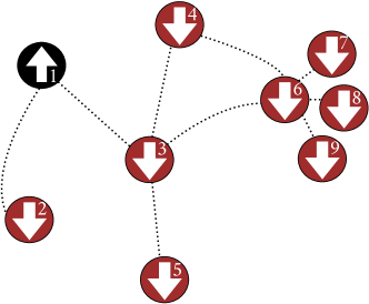
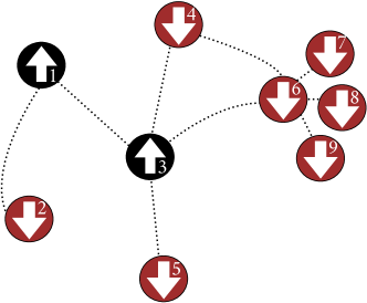
a)		b)

Figure 1: Agent configurations in epidemic process. In a), agent at vertex $k=1$ is infected. The graph configuration is $C_{1}=\lvert\uparrow\downarrow\downarrow\downarrow\downarrow\downarrow\downarrow\downarrow\downarrow\rangle$. In b), a second agent is infected at $k=3$, leading to the configuration $C_{5}=\lvert\uparrow\downarrow\uparrow\downarrow\downarrow\downarrow\downarrow\downarrow\downarrow\rangle$.

The next step required to assemble the transition matrix is the definition of operators and their actions on vectors in $\mathbbm{H}$. For instance, the operator $\hat{\sigma}^{z}_{k}$ probes whether the agent located at vertex $k$ is infected ($\uparrow$) or not ($\downarrow$):

$$\hat{\sigma}^{z}_{k}|\sigma_{1}\sigma_{2}\cdots\sigma_{N}\rangle=(\delta_{\sigma_{k}\uparrow}-\delta_{\sigma_{k}\downarrow})|\sigma_{1}\sigma_{2}\cdots\sigma_{N}\rangle,$$ (2)

while the operator $\hat{n}_{k}={(\hat{\sigma}^{z}_{k}+1)}/{2}$ extracts the number of infected agent at vertex $k$. Accordingly, the operator $\hat{n}=\sum_{k}\hat{n}_{k}$ extracts the total number of infected agents in the population. The $k$-th agent health status is switched by action of operators $\hat{\sigma}_{k}^{+}$ and $\hat{\sigma}_{k}^{-}$:

$$\hat{\sigma}_{k}^{+}\lvert\sigma_{1}\cdots\downarrow\cdots\sigma_{N}\rangle= \lvert\sigma_{1}\cdots\uparrow\cdots\sigma_{N}\rangle,$$ (3)

$$\hat{\sigma}_{k}^{-}\lvert\sigma_{1}\cdots\uparrow\cdots\sigma_{N}\rangle= \lvert\sigma_{1}\cdots\downarrow\cdots\sigma_{N}\rangle,$$ (4)

null otherwise. Another useful operator is $\hat{\sigma}_{k}^{x}=\hat{\sigma}_{k}^{+}+\hat{\sigma}_{k}^{-}$. The localized operators $\hat{\sigma}_{k}^{\pm}$ and $\hat{\sigma}_{k}^{z}$ satisfy additional algebraic properties. For each $k$, the set $\hat{\sigma}_{k}^{\pm,z}$ forms a local $\operatorname{su}(2)$ algebra, $[\hat{\sigma}_{k}^{z},\hat{\sigma}_{k}^{\pm}]=\pm 2\hat{\sigma}_{k}^{\pm}$, $[\hat{\sigma}_{k}^{+},\hat{\sigma}_{k}^{-}]=\sigma_{k}^{z}$ and $\{\hat{\sigma}_{k}^{+},\hat{\sigma}_{k}^{-}\}=1$. Note that $\sigma$ operators satisfy local fermionic anticommutation relations Lieb et al. (1961). However, their non-local algebraic commutation relations are bosonic: $[\hat{\sigma}_{k}^{\beta},\hat{\sigma}_{k^{\prime}}^{\gamma}]=0$, for $k\neq k^{\prime}$ and $\beta,\gamma=\pm,z$.

Let $P_{\mu}(t)$ be the probability to find the system in the configuration $\lvert C_{\mu}\rangle$, at time $t$. The collection of all $P_{\mu}(t)$ forms the probability vector, $\lvert P(t)\rangle=\sum_{\mu}P_{\mu}(t)\lvert C_{\mu}\rangle$, with $\sum_{\mu}P_{\mu}(t)=1$. For any Markov process, the transition matrix $\hat{T}$ describes allowed transitions among configurations such that $\lvert P(t+\delta t)\rangle=\hat{T}\lvert P(t)\rangle$. Under Poissonian assumption Pastor-Satorras et al. (2015), one only considers either a single cure or single infection event during a time interval $\delta t$. The Poissonian hypothesis tends to be more accurate for vanishing $\delta t$.

In the SIS model, any previously infected agent at vertex $k$ is subjected to three distinct outcomes during the time interval $\delta t$: transmit the disease to one connected susceptible agent; cure itself; or remain unchanged. The operator $\hat{\sigma}^{-}_{k}\hat{n}_{k}$ produces the desired cure action, while $A_{km}\hat{\sigma}^{+}_{m}\hat{n}_{k}$ transmits the disease from the $k$-th agent to $m$-th agent, given the $k$-th agent is currently infected and the other is susceptible, as exemplified for the fully connected graph depicted in Fig. 2.

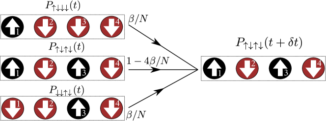
Figure 2: Markov process during the transmission phase. The probability $P_{\uparrow\downarrow\uparrow\downarrow}(t+\delta t)$ to find the system in the configuration $\lvert\uparrow\downarrow\uparrow\downarrow\rangle$, at time $t+\delta t$, depends on probability $P_{\uparrow\downarrow\downarrow\downarrow}(t)$ that the system was previously in the configuration $\lvert\uparrow\downarrow\downarrow\downarrow\rangle$ and then transitioned with conditional probability $p(\uparrow\downarrow\uparrow\downarrow|\uparrow\downarrow\downarrow\downarrow)=\beta/N$ to state $\lvert\uparrow\downarrow\uparrow\downarrow\rangle$. Analogous rationale applies to the configuration $\lvert\downarrow\downarrow\uparrow\downarrow\rangle$. The other possibility is that the system was already in the state $\lvert\uparrow\downarrow\uparrow\downarrow\rangle$ at time $t$ and remains unchanged during the time interval $\delta t$. As such, the probability to remain unchanged equals to one minus the probability to change to any other state. In this example, the graph is fully connected and there are $4$ such transitions.

If the cure and infection phases are independent from each other then $\hat{T}=\hat{T}_{\text{cure}}\hat{T}_{\text{infec}}$. Under this circumstances, the transition matrix is

$$\hat{T}=\mathbbm{1}-\frac{\beta}{N}\sum_{kj}\left[A_{jk}(1-\hat{n}_{j}-\hat{\sigma}^{+}_{j})+\Gamma\delta_{kj}(1-\hat{\sigma}^{-}_{j})\right]\hat{n}_{k},$$ (5)

with $\Gamma=\gamma N/\beta$. Once the explicit action of $\hat{T}$ is known, $P_{\mu}(t)$ are readily evaluated. Fig. 3 exhibits numerical results for $P_{\mu}(t)$ for $\mu=0,5,2^{N}-1$, parameter $\Gamma/N=0.0,0.1,0.3,0.5,1.2$, $P_{1}(0)=1$ as initial condition and $N=12$, in a fully connected network. For increasing $\Gamma/N$, the probability $P_{0}(t)$ to find the system without infected agents also increases, while the opposite holds true for $P_{2^{N}-1}(t)$, in which all agents are infected. The intermediate configuration $C_{5}$ is displayed to emphasize transient effects. Despite its simplicity, Eq. (5) produces power-law behavior, exemplified in Fig. 3 with $\Gamma/N=0.3,0.5$, in which the time interval to reach the stationary state $C_{0}$ is much larger than the total number of agents, $\Delta\tau\gg N\delta t$.

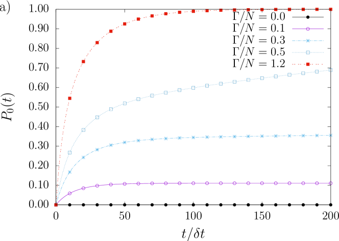
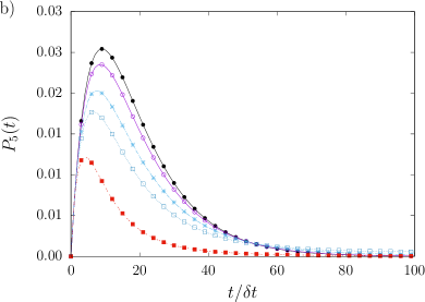
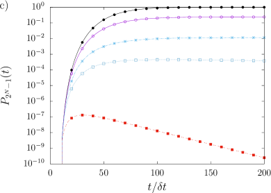
Figure 3: Configuration probabilities $P_{\mu}(t)$ for $\mu=0,5$ and $2^{N}-1$ with $N=12$ in a fully connected network. In a), probability $P_{0}(t)$ to observe all-cured configuration at time $t$ for various couplings $\Gamma/N$. In b), $P_{5}(t)$ refers to the probability of transient configuration $\lvert\uparrow_{1}\uparrow_{2}\downarrow_{3}\cdots\downarrow_{N}\rangle$, while c) exhibits the probability with all-infected agents, $P_{2^{N}-1}(t)$, in log scale. The coupling $\Gamma/N=0$ represents the SI model, whose stationary state is described by all-infected configuration. For $\Gamma/N=0.1$, the stationary state is a linear combination of distinct $C_{\mu}$, including all-cured $C_{0}$ and all-infected $C_{2^{N}-1}$ configurations. For intermediate couplings $\Gamma/N=0.3$ and $\Gamma/N=0.5$, the stationary state is $C_{0}$ with large transient $\Delta\tau\sim o(N^{4})$.

Brief inspection reveals $\hat{T}$ is asymmetric, thus implying the existence of distinct left and right eigenvectors.

Derivation of Eq. (5) considers only a single network realization. If an ensemble containing $M$ graphs is considered, properly sampling the network, the only modification required is the following: $A_{jk}\rightarrow\bar{A}_{jk}=M^{-1}\sum_{l=1}^{M}A_{jk}^{(l)}$. The reason is the following: networks only assign distribution rules for connections, leaving the vertex distribution and, therefore, the Hilbert space unchanged. For each graph $l=1,\ldots,M$ in the ensemble, one applies the associated transition matrix, $\hat{T}^{(l)}$, on the initial configuration $\lvert P^{(l)}(0)\rangle$, producing the probability vector $\lvert P^{(l)}(\delta t)\rangle$. In this way, one must also consider the ensemble averages. In particular, the average probability to find the system in configuration $\lvert C_{\mu}\rangle$ is $\langle P_{\mu}\rangle_{M}={M}^{-1}\sum_{l=1}^{M}{P_{\mu}^{(l)}(t)}$. Since the procedure is equivalent to the average of $\hat{T}$ over the graph ensemble – the network sample – one needs only to consider the network distribution of $A$. For clarity, we drop the bar symbol and always assume the average over graph ensemble.

II Squared Norm

Up to $O(\delta t^{2})$, $P_{\mu}(t)$ obeys the following system of differential equations,

$$\frac{dP_{\mu}}{dt}=-\sum_{\nu}H_{\mu\nu}P_{\nu}(t),$$ (6)

where $\hat{H}\equiv(\mathbbm{1}-\hat{T})/\delta t$ is the time generator. For time independent $\hat{H}$, $\lvert P(t)\rangle=\exp(-\hat{H}t)\lvert P(0)\rangle$ is the solution of Eq. (6). The operator $\hat{H}$ governs the dynamics with eigenvalues $\{\lambda_{\mu}\}$ and the respective left $\{\chi_{\mu}\}$ and right $\{\phi_{\mu}\}$ eigenvectors. The eigenvalues satisfy $\lambda_{\mu}\geq 0$, vanishing for stationary states van Kampen (1992). Statistics for observable $\hat{O}(t)$ are calculated according to $\langle O(t)\rangle=\sum_{\mu}\langle C_{\mu}|\hat{O}|C_{\mu}\rangle P_{\mu}(t)$. Among the relevant observables in disease spreading models, the mean number of infected agents, $\langle\hat{n}(t)\rangle$, and variance, $\sigma^{2}(t)$, exemplified in Fig. 4, are often relevant variables. Formally, they admit eigendecomposition: $\langle n(t)\rangle=\sum_{\mu\nu}\gamma_{\mu\nu}\mathrm{e}^{-\lambda_{\nu}t}$ and $\sigma^{2}(t)=\sum_{\mu\nu}\xi_{\mu\nu}\mathrm{e}^{-\lambda_{\nu}t}-\langle n(t)\rangle^{2}$, with $\gamma_{\mu\nu}=\langle C_{\mu}|\sum_{k}\hat{n}_{k}|C_{\mu}\rangle\langle C_{\mu}|\phi_{\nu}\rangle\langle\chi_{\nu}|P(0)\rangle$ and $\xi_{\mu\nu}=\langle C_{\mu}|\sum_{kl}\hat{n}_{k}\hat{n}_{l}|C_{\mu}\rangle\langle C_{\mu}|\phi_{\nu}\rangle\langle\chi_{\nu}|P(0)\rangle$.

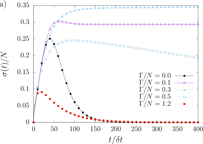
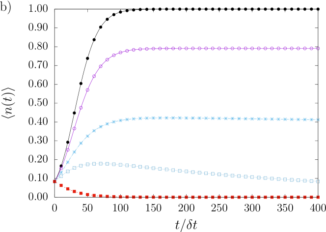
Figure 4: Standard deviation $\sigma(t)$ and mean $\langle n(t)\rangle$ for SIS model with $N=12$ in the fully connected network. The statistics $\sigma(t)$ and $\langle n(t)\rangle$ are shown in a) and b), respectively. Intermediate cure/infection rates $\Gamma/N=0.3$ and $\Gamma/N=0.5$ eradicate the disease after very large time intervals: $\sigma(t)$ exhibits initial rapid growth, develops a maximum at $t^{\prime}_{c}\equiv t^{\prime}_{c}(\Gamma/N)$ and then decays as power-law.

Although left and right eigenvectors are expected to decompose the identity, their actual computation is rather cumbersome, doubling the computational effort and are specially prone to convergence errors. They also lack a clear analytical interpretation. Here we consider the squared norm, $\lvert P(t)\rvert^{2}=\sum_{\mu}P_{\mu}^{2}$, which remains invariant under unitary transformations. First, total probability conservation $\sum_{\mu}P_{\mu}(t)=1$ does not warrant $|P(t)|^{2}$ conservation over time. Examples are found in Markov processes that evolve to unique stationary states since more configurations are available during the transient. The epidemic models considered in this study fall into this category, as shown in Fig. 5.

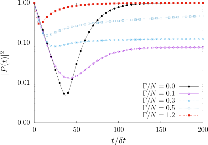
Figure 5: $|P(t)|^{2}$ in SIS model with $N=12$ and $P_{1}(0)=1$. For each coupling parameter $\Gamma/N$, $|P(t)|^{2}$ always develops a global minimum followed by constant value at stationary state, being unity only for single state configurations. Logarithmic scale is employed to emphasize extremal points at $t_{c}\equiv t_{c}(\Gamma/N)$.

Second, the time derivative of $\lvert P(t)\rvert^{2}$ is obtained from the hermitian operator $\hat{\mathcal{H}}=(1/2)(\hat{H}+\hat{H}^{T})$,

$$\frac{1}{2}\frac{d}{dt}\lvert P(t)\rvert^{2}=-\langle P(t)\rvert\hat{\mathcal{H}}\lvert P(t)\rangle.$$ (7)

Unlike $\hat{H}$, the operator $\hat{\mathcal{H}}$ has eigenvalues $\{\Lambda_{\mu}\}$ but the left eigenvectors are computed from right eigenvectors $\{\psi_{\mu}\}$ by simple Hermitian conjugation. The trade-off is that $\Lambda_{\mu}$ may assume negative values, as shown in Fig. 6, and the coefficients $\langle\psi_{\mu}|P(t)\rangle=g_{\mu}(t)$ are complex numbers. As such, the coefficients $g_{\mu}$ are not probabilities. Despite this shortcoming, the coefficients $g_{\mu}$ are used to evaluate configuration probabilities:

$$P_{\mu}(t)=\sum_{\nu}g_{\nu}(t)\langle C_{\mu}|\psi_{\nu}\rangle.$$ (8)

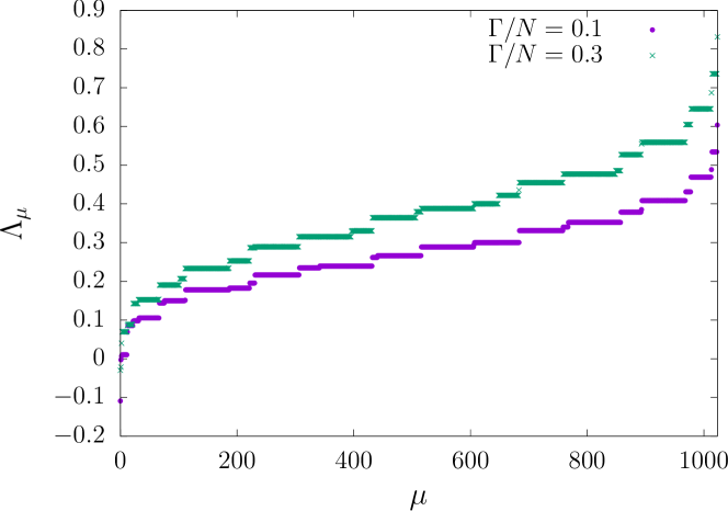
Figure 6: Sorted eigenspectra with $N=10$. Each filled circle (cross) represents one eigenvalue $\Lambda_{\mu}$ for coupling parameter $\Gamma/N=0.1$ ($0.3$).

An important expression is derived from Eq. (7),

$$\sum_{\mu}\left(\frac{1}{2}\frac{d}{dt}+\Lambda_{\mu}\right)|g_{\mu}(t)|^{2}=0,$$ (9)

subjected to the constraint $\sum_{\mu\nu}\langle C_{\mu}|\psi_{\nu}\rangle g_{\nu}(t)=1$. Now, Eq. (9) takes a simpler form if $\lvert P(t)\rvert^{2}$ is constant, which is the expected outcome whenever the system reaches at least one stationary state. In such case, Eq. (9) reads

$$\sum_{\mu}|\tilde{g}_{\mu,l}|^{2}\Lambda_{\mu}=0,$$ (10)

where the collection of coefficients $\tilde{g}_{\mu,l}\equiv\lim_{t\rightarrow\infty}g_{\mu}(t)$ describes the $l$-th stationary state. Table 1 displays Eq. (10) non-trivial solution for SI model with $N=3$ and $\beta/N=0.1$. This simple example is chosen since the solution can be evaluated by brute force and tested against the correct answer. Of course, the trivial solution $\tilde{g}_{\mu,0}=\delta_{\mu,0}$ and $\Lambda_{0}=0$ also satisfy Eq. (10).

Table 1: Stationary state. Non-vanishing coefficients $\tilde{g}_{\mu,1}$ in the SI model with $\beta/N=0.1$ and $N=3$. The set $\{\tilde{g}_{\mu,1}\}$ is obtained solving Eq. (10). The coefficients are real and $\tilde{g}_{\mu,1}=\langle C_{7}|\psi_{\mu}\rangle$, hence, $\tilde{P}_{7}=1$.

$\mu$	$\Lambda_{\mu}$	$\tilde{g}_{\mu,1}$
3	$0.157199(3)$	$0.397770(3)$
6	$0.351413(7)$	$-0.380366(0)$
7	$-0.108613(0)$	$0.834925(5)$

In addition to stationarity, $\lvert P(t)\rvert^{2}$ may also assume maximal or minimal values at time instants $t_{c}$, leading again to Eq. (10), the difference being only the evaluation of coefficients $g_{\mu}(t)$ at $t=t_{c}$. Numerical examples are shown in Fig. 7. The time instant $t_{c}$ is important for dynamics as the extremal condition $\lvert P(t_{c})\rvert^{2}$ informs us when the disease spreading rate changes its growth pattern. Accordingly, $t_{c}$ may also be used to estimate the maxima for narrow peaked statistics. For instance, the nonexistence of cure creates a rapid transient phase in SI model, with all agents infected as stationary state. During the transient, the variance $\langle n^{2}(t)\rangle-\langle n(t)\rangle^{2}$ is well described by a narrow function with peak near $t_{c}$. The estimation improves as $N$ increases. Therefore, by solving the constrained algebraic Eq. (10), either directly or via functional minimization, one also evaluates crucial statistics.

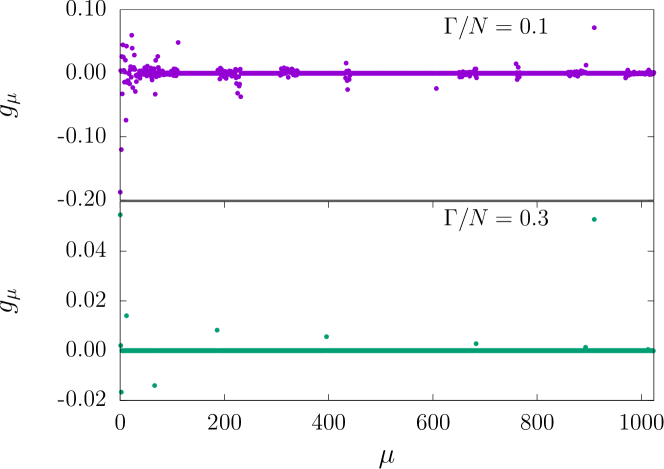
Figure 7: Solutions $g_{\mu}(t_{c})$ in SIS model with $N=10$. Non-trivial solutions to Eq. (10) are show for $\Gamma/N=0.1,\,0.3$. The coefficient distribution greatly differs depending on coupling parameter $\Gamma/N$.

We note Eqs. (9) and (10) introduce a novel way to tackle stochastic problems: asymmetric operators are replaced by symmetric operators and the eigenspectra are used to evaluate stationary states in Eq. (10). Furthermore, the stationary states obtained in this way carry the network topological information as the adjacency matrix determines the eigenvalue distribution. In the large $N\gg 1$ regime, the eigenspectrum becomes dense and it is convenient to analyze Eq. (9) using the continuous variable $\Lambda$. For completeness sake, we briefly discuss this regime in Appendix A. Alternatively, one may consider the extremal $|P(t_{c})|^{2}$ and obtain $t_{c}$. In turn, $t_{c}$ may be employed to estimate the time at which statistics develop maxima, as long as they are narrow peaked functions. Since the method is valid for any Markov process, it can be employed for more realistic epidemic models.

III Perturbation theory

The eigenvalues $\Lambda_{\mu}$ are crucial to Eq. (10) whereas the eigenvectors $\lvert\psi_{\mu}\rangle$ are required to ensure the probability conservation constraint. In this section, we consider small perturbations to the network link distribution and their corresponding effects on disease spreading in the SIS model.

For the SIS model, the Hermitian time generator is $\hat{\mathcal{H}}=(\beta/N)[\hat{\mathcal{H}}_{0}+\hat{\mathcal{H}}_{1}]$, with

$$\hat{\mathcal{H}}_{0}= \sum_{kj}A_{jk}\left[(1-\hat{n}_{j})\hat{n}_{k}-\frac{\hat{\sigma}_{j}^{+}\hat{n}_{k}+\hat{n}_{k}\hat{\sigma}^{-}_{j}}{2}\right],$$ (11)

$$\hat{\mathcal{H}}_{1}= \sum_{kj}{\Gamma\delta_{kj}\left(\hat{n}_{k}-\hat{\sigma}_{k}^{x}\right)}.$$ (12)

Here, the adjacency matrix elements $A_{jk}$ are the network average. The fully connected network is obtained taking $A_{jk}=(1-\delta_{jk})$ with mean field time generator $\hat{\mathcal{H}}_{\text{MF}}$. Despite its simplicity, this network provides relevant operatorial content. Defining the many-body spin operators as $S^{z}=\sum_{k}{\hat{n}_{k}}-N/2$, $S^{\pm}=\sum_{k}{\hat{\sigma}_{k}^{\pm}}$, and $S^{x}=\sum_{k}{(\hat{\sigma}_{k}^{+}+\hat{\sigma}_{k}^{-})/2}$, the resulting time generator is

$$\frac{\hat{\mathcal{H}}_{\text{MF}}}{\beta/N}= \frac{N}{2}\left[\frac{N}{2}-\Gamma\right]-\hat{S}^{z}\left[\hat{S}^{z}-\Gamma\right]+$$

$$- \frac{1}{2}\left\{\hat{S}^{x},\hat{S}^{z}\right\}-\hat{S}^{x}\left[\frac{N-1}{2}+\Gamma\right].$$ (13)

The operator $\hat{\mathcal{H}}_{\text{MF}}$ satisfies $[\hat{\mathcal{H}}_{\text{MF}},\hat{S}^{2}]=0$, where $\hat{S}^{2}=(\hat{S}^{z})^{2}+(1/2)\{\hat{S}^{+},\hat{S}^{-}\}$ is the Casimir operator. Thus, the eigenvalues $s(s+1)$ are suitable labels, with $s\geq 0$ and $s=N/2,N/2-1,\ldots$.

An important property is derived from the identification with many-body angular momentum operators. The operator $\hat{\mathcal{H}}_{\text{MF}}$ in Eq. (13) prohibits transitions among different $s$-sectors. This means the $\hat{\mathcal{H}}_{\text{MF}}$ is block diagonal, each block with dimension $d=2s+1$. In addition, each block is also tridiagonal in the basis $\lvert s,m\rangle$ ($m=-s,-s+1,\ldots,s$) as the $\hat{S}^{x}$ operator may only increase or decrease $m$ by unity. Therefore, the largest $s$-sector block has, at most, dimension $d_{\text{max}}=N+1$ and $3N-2$ non-null matrix elements, thus sparsity $O(3/N)$. When both properties are considered, one realizes the $O(2^{2N})$ computational problem has been reduced to $O(N)$. These properties eliminate one of the main obstacles faced by microscopic agent based epidemic models.

For general networks, the main strategy is to use the eigenvectors of $\hat{S}^{2}$ and treat any absent link among agents as perturbations. A simple perturbation to the fully connected topology is obtained by considering a small probability $\delta p\ll 1$ to independently remove links between vertices, $A_{jk}=(1-\delta_{jk})(1-\delta p)$. This procedure is equivalent to transform the underlying network into a random network Durrett (2010), with connection probability $1-\delta p$. Perturbative effects to $|P(t)|^{2}$ and $\sigma(t)$ are shown in Fig. 8. Although both network and topological perturbations are simple, distinct perturbative effects for increasing $\Gamma$ are observed.

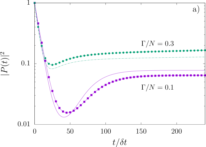
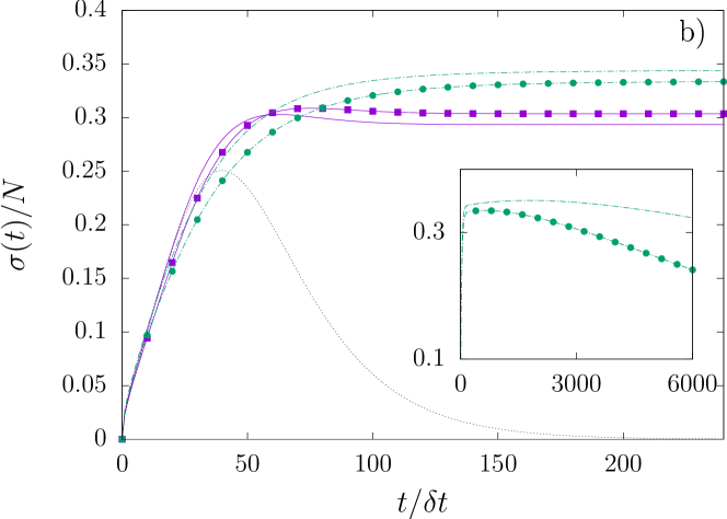
Figure 8: Perturbation in meanfield SIS model and $N=12$. In a), $|P(t)|^{2}$ is plotted against time steps for SIS coupling parameter $\Gamma/N=0.1$ in the meanfield network $\delta p=0$ (full magenta line) and in the perturbed network $\delta p=0.1$ (magenta squares); the corresponding quantities are also shown for $\Gamma/N=0.3$ with $\delta p=0$ (dashed green line) and $\delta p=0.1$ (green circles). Topological perturbations decrease (increase) $|P(t)|^{2}$ for $\Gamma/N=0.1$ ($0.3$). In b), $\sigma(t)$ is plotted against time steps. The dotted line displays the expected SI behavior for comparison. The inset shows $\sigma(t)$ with $\Gamma/N=0.3$ and $\delta p=0$ (dashed green line) and $\delta p=0.1$ ( green circles) using increased time range. During transients, small perturbations $\delta p$ may produce large modification to the statistics.

The perturbative operator is $-\delta p(\beta/N)\hat{V}$ where

$$\hat{V}=\left(\frac{N}{2}\right)^{2}-(\hat{S}^{z})^{2}-\left(\frac{N-1}{2}\right)\hat{S}^{x}-\frac{1}{2}\left\{\hat{S}^{z},\hat{S}^{x}\right\},$$ (14)

which is the SI symmetrized time generator and also satisfies $[\hat{V},\hat{S}^{2}]=0$.

Concerning stationary states, the first order correction to the eigenvalues, $\Lambda_{\mu}^{(1)}=\langle\psi_{\mu}|\hat{V}|\psi_{\mu}\rangle$, and eigenvectors, ${g}_{\mu}^{(1)}=\sum_{\nu}^{\prime}\langle\psi_{\mu}|\hat{V}|\psi_{\nu}\rangle/(\Lambda_{\nu}-\Lambda_{\mu})$, are obtained using standard perturbation theory Sakurai and Tuan (1994). Accordingly, first order correction to the probability to find the system in configuration $C_{\mu}$ is

$$P_{\mu}^{(1)}=\sum_{\nu}{\langle C_{\mu}|\psi_{\nu}\rangle{g}^{(1)}_{\nu}}.$$ (15)

Eq. (15) emphasizes the role played by the Hermitian operators $\hat{\mathcal{H}}$ to evaluate the effects caused by topological perturbations: $P^{(1)}_{\mu}$ and further perturbative corrections are entirely evaluated from eigenvectors $\{\lvert\psi_{\mu}\rangle\}$ and eigenvalues $\{\Lambda_{\mu}\}$, given the perturbation $\hat{V}$. This rationale suits decision making strategies as the only concern is the impact of changes to the system topology. The advantage in our approach lies in avoiding computations of the asymmetric operator $\hat{H}$ while benefiting from standard perturbative techniques.

IV Regular network

Fully connected networks are the simplest instances of a larger set known as regular networks. Other relevant element in the same set is obtained when the connection patterns among vertices are periodic. Lattices are their spatial representation and are widely employed to describe translation invariant systems. Their natural eigenset contains long and short range modes, allowing analytical tools to inspect long and short range disease spreading behavior, their characteristic frequencies and long range correlations. Since perturbative effects are our main concern here, we only consider a network with single period, or equivalently, a one-dimensional lattice of size $N$ with periodic boundary condition, as Fig. 9a) illustrates. The adjacency matrix is $A_{P}$ and the matrix elements are $(A_{P})_{kk^{\prime}}=(\delta_{k,k^{\prime}+1}+\delta_{k,k^{\prime}-1})$, with $V_{0}=V_{N}$ and $V_{N+1}=V_{1}$.

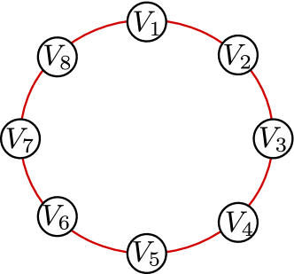
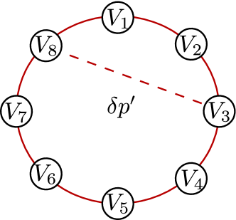
a)		b)

Figure 9: One-dimensional periodic lattice with $N=8$ vertices. a) Vertex $V_{k}$ connects with vertex $V_{k+1}$ and $V_{k-1}$ with periodic boundary conditions, $V_{N+1}=V_{1}$ and $V_{0}=V_{N}$. Perturbative link addition with probability $\delta p=\delta p^{\prime}/(1+\delta p^{\prime})$ increases the mean degree $d(k)$ by $p(N-2)$, allowing long range disease transmissions. In b), the graph shows the regular connections for $V_{3}$ and an additional connection to $V_{8}$.

The perturbative scheme to the network topology adds connections with probability $\delta p\ll 1$ among vertices not previously connected, as shown in Fig. 9b). The perturbation creates shortcuts throughout the network, favoring rapid disease dispersion, in an attempt to mimic the relevant aspects found in small-world networks Watts and Strogatz (1998). For a single graph realization, translation invariance breaks and the important expression $N^{-1}\sum_{k}\langle\hat{O}_{k}\rangle=\langle\hat{O}_{1}\rangle$ is no longer valid for a general observable $\hat{O}_{k}$. However, for a large ensemble of graphs, the average transition matrix recovers translation invariance. The reasoning behind this claim lies in the fact all vertices would have $2+\delta p(N-2)$ neighbors, on average.

Let $p_{k,k^{\prime}}=\delta p$ be the probability to create a single link between $V_{k}$ and $V_{k^{\prime}}$, including nearest-neighbor vertices. Clearly, the idea is to emphasize the emergence of translation invariance and to interpret the perturbation operator as the meanfield disease spreading operator $\hat{V}$ in Eq. (14). Under this assumption, the contributions to the adjacency matrix due to perturbations are $\delta p(1-\delta_{kk^{\prime}})$. One must be careful to subtract contributions from links already accounted by $A_{P}$, resulting in the symmetric time generator $\hat{\mathcal{H}}_{P}=(\beta/N)[(1-\delta p)\hat{\mathcal{H}}_{0}+\hat{\mathcal{H}}_{1}+\delta p\hat{V}]$. Next, define the effective couplings $\beta^{\prime}=(1-\delta p)\beta$ and $\delta p^{\prime}=\delta p/(1-\delta p)$, so that

$$\frac{\hat{\mathcal{H}}_{P}}{\beta^{\prime}/N}=\hat{\mathcal{H}}_{0}+\hat{\mathcal{H}}_{1}+\delta p^{\prime}\left(\hat{V}-\hat{\mathcal{H}}_{1}\right),$$ (16)

i.e., the perturbation operator is proportional to $\delta p^{\prime}$. The solution for $\delta p^{\prime}=0$ is obtained using techniques from strongly correlated systems and spinchains, in momentum space Lieb et al. (1961); Alcaraz and Nakamura (2010). Moreover, total momentum $Q=0,1,\ldots,N-1$ is conserved and serves as a label, breaking $\hat{\mathcal{H}}_{P}$ into $N$ block-diagonal matrices. For very large $\delta p$, the network topology moves towards meanfield topology and favors perturbative analysis using Eq. (13) as the unperturbed operator. Therefore, for $\delta p\ll 1$, the perturbative regime favors periodic eigenvectors whereas for $(1-\delta p)\ll 1$, many-body angular momentum eigenvectors are preferred.

V Bethe-Peierls approximation

In general, perturbations to topology are not required to affect all vertices in the same manner. For instance, consider a network whose links are distributed according to a parametric probability density function $p(\omega)$. If the network undergoes a parameter change $\omega\rightarrow\omega+\delta\omega$, one may expect ${A}_{ij}\rightarrow{A}_{ij}+\delta\omega\,G_{ij}$. The matrix $G$ carries all modifications experienced by the network under the change. Accordingly, the symmetric time generator is $\hat{\mathcal{H}}=(\beta/N)(\hat{\mathcal{H}}_{0}+\hat{\mathcal{H}}_{1}+\delta\omega\hat{V}^{G})$. The perturbation $\hat{V}^{G}$ is

$$\hat{V}^{G}=\frac{1}{2}\sum_{kj}G_{jk}\left[2(1-\hat{n}_{j})\hat{n}_{k}-\hat{\sigma}_{j}^{+}\hat{n}_{k}-\hat{n}_{k}\hat{\sigma}_{j}^{-}\right].$$ (17)

Hermiticity is sufficient to warrant Rayleigh–Schrödinger perturbation theory. Furthermore, Eq. (10) requires first order perturbative corrections $\Lambda_{\mu}^{(1)}$ and $g_{\mu}^{(1)}$ must satisfy

$$\sum_{\mu}\left[2\text{Re}(g_{\mu}^{*}g_{\mu}^{(1)})\Lambda_{\mu}+|g_{\mu}|^{2}\Lambda_{\mu}^{(1)}\right]=0.$$ (18)

Here, as usual, $\Lambda_{\mu}^{(1)}=\langle\psi_{\mu}|\hat{V}|\psi_{\mu}\rangle$ and $g_{\mu}^{(1)}=\sum_{\nu}^{\prime}\lvert\langle\psi_{\mu}|\hat{V}|\psi_{\nu}\rangle\rvert/(\Lambda_{\nu}-\Lambda_{\mu})$.

In addition to perturbative methods, analytical and numerical techniques from many-body theories are now available to epidemic models. This is also true for approximations, such as Bethe-Peierls Bethe (1935). In this approximation, $\hat{n}_{k}$ is replaced by global average $\bar{n}$. Application to the SIS model in an arbitrary network produces the effective time generator

$$\frac{2\hat{\mathcal{H}}^{\prime}}{\beta/N}=\Gamma N+\bar{n}\sum_{j}\kappa_{j}+\sum_{j}\Omega_{j}({\cos\theta_{j}\hat{\sigma}^{z}_{j}-\sin\theta_{j}\hat{\sigma}^{x}_{j}}),$$ (19)

where $\kappa_{j}=\sum_{k}{A}_{kj}$ is the degree of $j$-th vertex, $\Omega_{j}=\sqrt{2(\Gamma^{2}+\bar{n}^{2}\kappa_{j}^{2})}$, $\cos\theta_{j}=(\Gamma-\bar{n}\kappa_{j})/\Omega_{j}$ and $\sin\theta_{j}=(\Gamma+\bar{n}\kappa_{j})/\Omega_{j}$. The effective generator in Eq. (19) is diagonalized by rotations around the $y$-axis.

VI Conclusion

In compartmental approaches to epidemics, the role of fluctuactions is underestimated when the population of infected agents is scarce. Disease spreading models using agent based models are limited to small population sizes due to asymmetric time generators and their large $O(2^{2N})$ dimensions. Our findings show $\lvert P(t)\rvert^{2}$ is sufficient to avoid the mathematical hardships that accompany asymmetric operators. The squared norm provides a novel way to obtain stationary states and extremal configurations in general Markov processes, including epidemic models. Once stationary states are secured, the standard Rayleigh-Schrödinger perturbative technique becomes available to epidemics, making use of symmetrized operators and their eigenvalues and eigenvectors. The method paves the way for evaluation of corrections to configuration probabilities caused by perturbations in complex topologies, where analytical results are scarce.

Appendix A Continuous spectral equation

In the large $N\gg 1$ regime, the eigenspectra becomes dense and it is convenient to analyze Eq. (9) using the continuous variable $\Lambda$. Let $\rho(\Lambda)$ be the density of states between $\Lambda$ and $\Lambda+\delta\Lambda$. In addition, consider the real spectral functions $\eta_{1}(\Lambda,t)$ and $\eta_{2}(\Lambda,t)$ so that $g_{\mu}(t)\rightarrow\eta_{1}(\Lambda,t)+\imath\,\eta_{2}(\Lambda,t)$, with squared norm $\eta^{2}(\Lambda,t)\equiv\eta_{1}^{2}(\Lambda,t)+\eta_{2}^{2}(\Lambda,t)$. Since the time evolution of $\lvert P(t)\rvert^{2}$ is deterministic, it is convenient to define the functional $S[P]$ over a time interval $t_{1}-t_{0}$,

$$S[P]=\int_{t_{0}}^{t_{1}}dt\,\lvert P(t)\rvert^{2},$$ (20)

with

$$\lvert P(t)\rvert^{2}=\int_{-\infty}^{\infty}d\Lambda\rho(\Lambda)\eta^{2}(\Lambda,t).$$ (21)

Equation (20) suggests the interpretation of $S[P]$ as the system action. Let the underlying network link distribution be a continuous function of the real parameter $q$. Next, one considers virtual variations $\delta q$ to $q$, which produce the change $\delta\rho(\Lambda,t)$ in the density of states. According to Eq. (9), the continuous variables $\Lambda$ and real functions $\rho$ and $\eta$ satisfy the following spectral equation:

$$\int_{-\infty}^{\infty}d\Lambda\,\left(\frac{1}{2}\frac{\partial}{\partial t}+\Lambda\right)\rho(\Lambda)\eta^{2}(\Lambda,t)=0.$$ (22)

References

- de Espíndola et al. (2011) A. L. de Espíndola, C. T. Bauch, B. C. T. Cabella, and A. S. Martinez, “An agent-based computational model of the spread of tuberculosis,” J. Stat. Mech. Theor. Exp. 2011, P05003 (2011).
- Kermack and McKendrick (1991) W. O. Kermack and A. G. McKendrick, “Contributions to the mathematical theory of epidemics—i,” Bull. Math. Biol. 53, 33–55 (1991).
- Pastor-Satorras et al. (2015) R. Pastor-Satorras, C. Castellano, P. Van Mieghem, and A. Vespignani, “Epidemic processes in complex networks,” Rev. Mod. Phys. 87, 925–979 (2015).
- Heesterbeek et al. (2015) H. Heesterbeek, R. M. Anderson, V. Andreasen, S. Bansal, D. De Angelis, C. Dye, K. T. D. Eames, W. J. Edmunds, S. D. W. Frost, S. Funk, T. D. Hollingsworth, T. House, V. Isham, P. Klepac, J. Lessler, J. O. Lloyd-Smith, C. J. E. Metcalf, D. Mollison, L. Pellis, J. R. C. Pulliam, M. G. Roberts, and C. Viboud, “Modeling infectious disease dynamics in the complex landscape of global health,” Science 347 (2015).
- Bansal et al. (2007) S. Bansal, B. T. Grenfell, and L. A. Meyers, “When individual behaviour matters: homogeneous and network models in epidemiology,” J. R. Soc. Interface 4, 879–891 (2007).
- Heffernan et al. (2005) J.M Heffernan, R.J Smith, and L.M Wahl, “Perspectives on the basic reproductive ratio,” J. R. Soc. Interface 2, 281–293 (2005).
- Eames and Keeling (2002) K. T. D. Eames and M. J. Keeling, “Modeling dynamic and network heterogeneities in the spread of sexually transmitted diseases,” Proc. Natl. Acad. Sci. USA 99, 13330–13335 (2002).
- Aiello and da Silva (2003) O.E. Aiello and M.A.A. da Silva, “New approach to dynamical monte carlo methods: application to an epidemic model,” Physica A 327, 525 – 534 (2003).
- Haas et al. (1999) V.J. Haas, A. Caliri, and M.A.A. da Silva, “Temporal duration and event size distribution at the epidemic threshold,” J. Biol. Phys. 25, 309–324 (1999).
- Keeling and Eames (2005) M.J. Keeling and K.T.D Eames, “Networks and epidemic models,” J. R. Soc. Interface 2, 295–307 (2005).
- Albert and Barabási (2002) R. Albert and A.-L. Barabási, “Statistical mechanics of complex networks,” Rev. Mod. Phys. 74, 47–97 (2002).
- van Kampen (1992) N. G. van Kampen, Stochastic Processes in Physics and Chemistry, Vol. 1 (Elsevier Science, Amsterdam, 1992).
- Lieb et al. (1961) E. Lieb, T. Schultz, and D. Mattis, “Two soluble models of an antiferromagnetic chain,” Ann. Phys. (N.Y.) 16, 407 – 466 (1961).
- Durrett (2010) R. Durrett, “Some features of the spread of epidemics and information on a random graph,” Proc. Natl. Acad. Sci. USA 107, 4491–4498 (2010).
- Sakurai and Tuan (1994) J. J. Sakurai and S. F. Tuan, Modern quantum mechanics (Addison-Wesley, 1994).
- Watts and Strogatz (1998) D. J. Watts and S. H. Strogatz, “Collective dynamics of small-world networks,” Nature 393, 440–442 (1998).
- Alcaraz and Nakamura (2010) F. C. Alcaraz and G. M. Nakamura, “Phase diagram and spectral properties of a new exactly integrable spin-1 quantum chain,” J. Phys. A: Math. Gen. 43, 155002 (2010).
- Bethe (1935) H. A. Bethe, “Statistical theory of superlattices,” Proc. R. Soc. A 150, 552–575 (1935).