Casimir free energy and pressure for magnetic metal films

Abstract

We examine the Casimir free energy and pressure of magnetic metal films, which are free-standing in vacuum, sandwiched between two dielectric plates, and deposited on either nonmagnetic or magnetic metallic plates. All calculations are performed using both the Drude and plasma model approaches to the Lifshitz theory. According to our results, the Casimir free energies and pressures calculated using both theoretical approaches are significantly different in the magnitude and sign even for thin films of several tens of nanometers thickness. Thus, for the Ni film of 47 nm thickness deposited on a Fe plate the obtained magnitudes of the Casimir free energy differ by the factor of 5866. We show that the Casimir free energy and pressure of a magnetic film calculated using the plasma model approach do not possess the classical limit, but exponentially fast drop to zero with increasing film thickness. If the Drude model approach is used, the classical limit is reached for magnetic films of about 150 nm thickness, but the Casimir free energy remains nonzero in the limit of ideal metal, contrary to expectations. For the plasma model approach the Casimir free energy of a film vanishes in this case. Numerical computations are performed for the magnetic films made of Ni, nonmagnetic plates made of Cu and Al, and magnetic plates made of Fe using the tabulated optical data for the complex indexes of refraction of all metals. The obtained results can be used for a discrimination between the plasma and Drude model approaches in the Casimir physics and in the investigation of stability of thin films.

I Introduction

The physical phenomena caused by the electromagnetic fluctuations attract increasing attention because they are closely connected with the basics of quantum statistical physics and simultaneously are important for many innovative technologies. The most well known fluctuation-induced phenomenon is the van der Waals force 1 acting at short separations between two uncharged particles, a particle and a macrobody and between two macrobodies. Its relativistic analogue, the Casimir force 2 , has also received much publicity in connection with the zero-point fluctuations of quantized fields, although this effect originates from the thermal fluctuations as well. Both forces are often mentioned under a generic name of dispersion forces.

In spite of many applications of the Casimir effect in atomic physics 3 ; 4 ; 5 ; 6 ; 7 ; 8 , condensed matter physics 9 ; 10 ; 11 ; 12 ; 13 ; 14 and nanotechnology 15 ; 16 ; 17 ; 18 ; 19 , the most important outcome is, probably, that it sheds new light on the interaction of quantum fluctuations with matter and the role of dissipation in this process 20 . Specifically, it was shown 21 ; 22 ; 23 ; 23a ; 24 that if the dielectric response of metals with perfect crystal lattices is described by the dissipative Drude model (as is certainly true in real electromagnetic fields with a nonzero expectation value, but is usually applied to fluctuating fields with zero expectation value as well) the Lifshitz theory of dispersion forces comes into conflict with the third law of thermodynamics, the Nernst heat theorem. Note that when the spatially nonlocal dielectric response is considered, the Nernst heat theorem is satisfied 25a . The reason is that effects of spatial dispersion lead to an effective nonzero residual relaxation. This, however, does not solve the problem. The point is that at sufficiently short separations between the Casimir plates the frequency region of infrared optics, where the dielectric response is local, plays an important role. It was shown that if the frequency regions with both nonlocal and local response functions are taken into account, the Nernst heat theorem is again violated 25b .

In parallel with this, several precise experiments performed by two experimental groups demonstrated that measurements of the Casimir interaction between both nonmagnetic and magnetic test bodies exclude theoretical predictions of the Lifshitz theory taking into account dissipation of free electrons at up to 99% confidence level 25 ; 26 ; 27 ; 28 ; 29 ; 30 ; 31 . The same experimental data were found in agreement with the Lifshitz theory if the free electrons are described by the nondissipative plasma model 25 ; 26 ; 27 ; 28 ; 29 ; 30 ; 31 at more than 90% confidence level 32 . Note that the magnetic response falls so rapidly with increasing frequencies 53 that the magnetic permeability is effectively unity for all nonzero-frequency Matsubara terms of the Lifshitz formula and takes its static value for the zero-frequency Matsubara term only 54 . It was shown also 21 ; 22 ; 23 ; 23a ; 24 that the Lifshitz theory satisfies the Nernst theorem for both nonmagnetic and magnetic materials if the plasma model is used in place of the Drude one.

At separations below $1\,\mu$m between the test bodies, where the experiments of Refs. 25 ; 26 ; 27 ; 28 ; 29 ; 30 ; 31 are the most precise, the differences in theoretical predictions using the Drude and plasma models do not exceed a few percent. Because of this, it has been argued on occasion that the obtained results might be not conclusive. Recently, however, several differential Casimir experiments exploiting magnetic metals have been proposed 33 ; 34 ; 35 , where the theoretical predictions using the Drude and plasma models at low frequencies differ by up to a factor of 1000. One of these experiments 36 ; 36a has already demonstrated with certainty that the Drude model approach is excluded by the data, whereas the plasma model approach was found to be consistent with the same data.

In addition to experiments with metallic test bodies, several precision measurements of the Casimir and Casimir-Polder force with dielectric test bodies have been made 37 ; 38 ; 39 ; 40 . The experimental data were found in agreement with theoretical predictions of the Lifshitz theory only under a condition that the contribution of free charge carriers to the dielectric permittivity is disregarded in calculations. If the free charge carriers are taken into account, the computational results are excluded by the data at up to 95% confidence level 37 ; 38 ; 39 ; 40 ; 41 . It was proved also that for dielectric materials the Lifshitz theory violates the Nernst heat theorem if the free charge carriers at nonzero temperature are taken into account and satisfies it if the free charge carriers are disregarded 23a ; 42 ; 43 ; 44 ; 45 ; 46 .

Recently a new type of the Casimir experiments was proposed which allows an immediate discrimination between the Drude and plasma model approaches without resorting to the differential force measurements 47 . It was shown 47 that the Casimir free energy and pressure of a nonmagnetic metallic film with less than 100 nm thickness can differ up to a factor of several tens when it is calculated using different theoretical approaches. In so doing, this film can be either a free-standing or sandwiched between two dielectric plates. Similar results have been obtained for nonmagnetic metal films deposited on the plates made of nonmagnetic metals 49a . Note that the clarification of a question what is the van der Waals and Casimir energy of metallic films is interesting not only from the theoretical point of view. The matter is that these interactions are important for the problem of stability of thin films and should be taken into account in numerous applications 48 .

In this paper, we investigate the Casimir free energy and pressure of thin films made of magnetic metal. Interest to this subject is motivated by the recent experiments on measuring the Casimir force between magnetic test bodies 30 ; 31 ; 36 ; 36a ; 49 and the great role played by magnetic coatings in various applications. We consider the Casimir free energy and pressure of a magnetic film either a free-standing or sandwiched between two dielectric plates. We also calculate the Casimir free energy and pressure of magnetic films deposited on either nonmagnetic or magnetic metal plates. All calculations are performed using both the Drude and plasma model approaches, and in all cases important differences in the obtained results are revealed.

Specifically, if the Drude model approach is used, the Casimir free energy and pressure have the classical limit, which is already reached for thin films of about 150 nm thickness. Recall that in the classical limit the Casimir free energy and pressure become essentially classical, i.e., the main contributions to them do not depend on the Planck constant. For two metallic plates separated by a vacuum gap the classical limit is reached at much larger separations (higher temperatures). The Casimir free energy and pressure of a film calculated using the plasma model approach do not have the classical limit, i.e., the main contributions to them remain dependent on the Planck constant for any film thickness. In this case the Casimir free energy and pressure decrease to zero exponentially fast with increasing thickness of the film. Because of this, even for thin films of a few tens of nanometers thickness, the difference in theoretical predictions of both approaches reaches hundreds and thousands percent. This allows an experimental discrimination between different predictions do not using the differential force measurements. According to our results, in the limiting case of ideal metal the Casimir free energy and pressure of a magnetic metal film calculated using the Drude model approach do not go to zero. It is in conflict with intuition if to take into account that the electromagnetic fluctuations cannot penetrate in an interior of ideal metal. The plasma model approach is shown to be in accordance with this demand.

Numerical computations are performed for a Ni film free-standing in vacuum or sandwiched between two sapphire plates. We have also computed the Casimir free energy and pressure of the magnetic Ni film deposited on a nonmagnetic plate made of Cu or Al and a magnetic plate made of Fe. All computations are performed using the complete optical data of all metals under consideration extrapolated to zero frequency by either the Drude or the plasma model. It is shown that for Ni films deposited on Al or Cu plates the Casimir free energy and pressure calculated using the plasma model approach are positive (i.e., correspond to the Casimir repulsion). If the Drude model approach is used, the Casimir free energy and pressure change their sign with increasing film thickness. For a Ni film deposited on a Fe plate the Casimir free energy and pressure are positive if the Drude model approach is used in calculations and change their sign with increasing film thickness if one uses the plasma model approach.

The paper is organized as follows. In Sec. II the general formalism is presented and the dielectric functions of all considered metals along the imaginary frequency axis are displayed. Section III is devoted to a magnetic metal film in vacuum or sandwiched between two dielectrics. In Sec. IV we consider a magnetic metal film deposited on nonmagnetic metal plates. In Sec. V a magnetic metal film deposited on a magnetic metal plate is considered. Section VI contains our conclusions and discussion.

II General formalism

We consider a magnetic metal film of thickness $a$ characterized by the frequency-dependent dielectric permittivity $\varepsilon^{(2)}(\omega)$ and magnetic permeability $\mu^{(2)}(\omega)$. This film may be sandwiched between two thick plates (semispaces) described by the quantities $\varepsilon^{(1)}(\omega),\,\,\mu^{(1)}(\omega)$ and $\varepsilon^{(3)}(\omega),\,\,\mu^{(3)}(\omega)$. If these plates are nonmagnetic, the equalities $\mu^{(1)}(\omega)=\mu^{(3)}(\omega)=1$ hold. For a free-standing film in vacuum one also has $\varepsilon^{(1)}(\omega)=\varepsilon^{(3)}(\omega)=1$. Finally, for a film deposited on a plate we have $\varepsilon^{(3)}(\omega)=\mu^{(3)}(\omega)=1$. The Casimir free energy per unit area of our magnetic film at temperature $T$ in thermal equilibrium with an environment is given by the Lifshitz formula 1 ; 2 ; 51 ; 52

$${\cal F}(a,T)=\frac{k_{B}T}{2\pi}\sum_{l=0}^{\infty}{\vphantom{\sum}}^{\prime}\int_{0}^{\infty}k_{\bot}\,dk_{\bot}\sum_{\alpha}\ln\left[1-r_{\alpha}^{(2,3)}(i\xi_{l},k_{\bot})r_{\alpha}^{(2,1)}(i\xi_{l},k_{\bot})e^{-2ak_{l}^{(2)}(k_{\bot})}\right],$$ (1)

where, $k_{B}$ is the Boltzmann constant, $k_{\bot}=|\mbox{\boldmath$k$}_{\bot}|$ is the magnitude of the projection of the wave vector on the surface of the film, and the prime on a summation sign over $l$ multiplies the term with $l=0$ by 1/2. The second summation is over two independent polarizations of the electromagnetic field, transverse magnetic ($\alpha={\rm TM}$) and transverse electric ($\alpha={\rm TE}$). The respective reflection coefficients calculated at the pure imaginary Matsubara frequencies $\xi_{l}=2\pi k_{B}Tl/\hbar$, $l=0,\,1,\,2,\,\ldots$, are given by

$$r_{\rm TM}^{(2,n)}(i\xi_{l},k_{\bot})=\frac{\varepsilon_{l}^{(n)}k_{l}^{(2)}(k_{\bot})-\varepsilon_{l}^{(2)}k_{l}^{(n)}(k_{\bot})}{\varepsilon_{l}^{(n)}k_{l}^{(2)}(k_{\bot})+\varepsilon_{l}^{(2)}k_{l}^{(n)}(k_{\bot})},$$

$$r_{\rm TE}^{(2,n)}(i\xi_{l},k_{\bot})=\frac{\mu_{l}^{(n)}k_{l}^{(2)}(k_{\bot})-\mu_{l}^{(2)}k_{l}^{(n)}(k_{\bot})}{\mu_{l}^{(n)}k_{l}^{(2)}(k_{\bot})+\mu_{l}^{(2)}k_{l}^{(n)}(k_{\bot})},$$ (2)

where

$$k_{l}^{(n)}(k_{\bot})=\sqrt{k_{\bot}^{2}+\mu_{l}^{(n)}{\varepsilon_{l}^{(n)}}\frac{\xi_{l}^{2}}{c^{2}}},$$ (3)

$\mu_{l}^{(n)}\equiv\mu^{(n)}(i\xi_{l})$, $\varepsilon_{l}^{(n)}\equiv\varepsilon^{(n)}(i\xi_{l})$, and $n=1,\,2,\,3$.

As is mentioned in Sec. I, the magnetic permeabilities of metals along the imaginary frequency axis decrease with increasing frequency and at room temperature $T=300\,$K drop to unity at much lower frequencies than the first Matsubara frequency 53 ; 54 . This means that in all terms of Eq. (1) with $l\geq 1$ one can put $\mu_{l}^{(n)}=1$. As a result, in all terms of Eq. (1) with $l\geq 1$ the reflection coefficients preserve their form (2) where one should put

$$k_{l}^{(n)}(k_{\bot})=\sqrt{k_{\bot}^{2}+{\varepsilon_{l}^{(n)}}\frac{\xi_{l}^{2}}{c^{2}}},\quad\mu_{l}^{(n)}=1.$$ (4)

The reflection coefficients at $l=0$ take different forms depending on the configuration under consideration. They are presented in the following sections. Here we only notice that for the magnetic films made of Ni and magnetic plates made of Fe we have 55

$$\mu_{0}^{(2)}\equiv\mu_{\rm Ni}=110,\quad\mu_{0}^{(1)}\equiv\mu_{\rm Fe}=10^{4}.$$ (5)

To perform computations of the Casimir free energy using Eq. (1), one also needs the values of dielectric permittivities at the imaginary Matsubara frequencies. In the next sections we consider Ni and Pt films and Al, Cu, and Fe plates. The dielectric permittivities for all of them along the imaginary frequency axis were obtained from the tabulated optical data for the complex index of refraction 50 using the Kramers-Kronig relation. The respective procedure is described in detail in Refs. 2 ; 52 for the case of Au. In the literature, there are some alternative sets of optical data for metal films which also depend on a specific sample used. Our results below, however, are almost independent on what set of optical data is used in computations. An extrapolation of the optical data down to zero frequency was performed using both the Drude and plasma models

$$\varepsilon_{D}(i\xi)=1+\frac{\omega_{p}^{2}}{\xi_{l}(\xi_{l}+\gamma)},\quad\varepsilon_{p}(i\xi)=1+\frac{\omega_{p}^{2}}{\xi_{l}^{2}},$$ (6)

where $\omega_{p}$ is the plasma frequency and $\gamma$ is the relaxation parameter, for the reasons described in Sec. I. Note that both these dielectric permittivities considered in the complex frequency plane satisfy the Kramers-Kronig relations formulated for functions having the first- and second-order poles at zero frequency, respectively 2 ; 52 .

In Fig. 1(a) the obtained dielectric permittivities of Ni and Pt (in the inset) are shown as functions of the imaginary frequency normalized to the first Matsubara frequency at room temperature $\xi_{1}=2.468\times 10^{14}\,\mbox{rad/s}=0.1624\,$eV. The upper and lower solid lines plotted in the double logarithmic scale are obtained using the plasma and Drude extrapolations, respectively. The plasma frequencies and relaxation parameters used in the extrapolations are $\omega_{p,{\rm Ni}}=4.89\,$eV, $\gamma_{\rm Ni}=0.0436\,$eV 50 ; 56 , and $\omega_{p,{\rm Pt}}=4.94\,$eV, $\gamma_{\rm Pt}=0.13\,$eV (close to Ref. 56 ), respectively. For Al, Cu, and Fe the dielectric permittivities along the imaginary frequency axis are presented in Fig. 1(b) in a similar way. The following plasma frequencies and relaxation parameters were used in the extrapolations: $\omega_{p,{\rm Al}}=11.34\,$eV, $\gamma_{\rm Al}=0.041\,$eV (close to Ref. 57 ), $\omega_{p,{\rm Cu}}=8.6\,$eV, $\gamma_{\rm Cu}=0.0325\,$eV (close to Ref. 56 ), and $\omega_{p,{\rm Fe}}=4.09\,$eV, $\gamma_{\rm Fe}=0.018\,$eV 56 . As is seen in Fig. 1(a,b), the most important impact from different extrapolations is given only by the first Matsubara frequency.

In the next section we also consider the magnetic Ni film sandwiched between two sapphire plates. The dielectric permittivity of sapphire along the imaginary frequency axis admits rather precise analytic expression 58

$$\varepsilon_{s}(i\xi)=1+\frac{C_{\rm IR}\omega_{\rm IR}^{2}}{\omega_{\rm IR}^{2}+\xi^{2}}+\frac{C_{\rm UV}\omega_{\rm UV}^{2}}{\omega_{\rm UV}^{2}+\xi^{2}},$$ (7)

where $C_{\rm UV}=2.072$, $C_{\rm IR}=7.03$, $\omega_{\rm UV}=2.0\times 10^{16}\,$rad/s, and $\omega_{\rm IR}=1.0\times 10^{14}\,$rad/s. This permittivity was recently used in Ref. 47 and is used below as well.

In the end of this section we present the Lifshitz formula for the Casimir pressure for a magnetic metal film included in the same configurations, as described above. It is a direct consequence of Eq. (1):

$$P(a,T)=-\frac{k_{B}T}{\pi}\sum_{l=0}^{\infty}{\vphantom{\sum}}^{\prime}\int_{0}^{\infty}k_{\bot}k_{l}^{(2)}(k_{\bot})\,dk_{\bot}\sum_{\alpha}\left[\frac{e^{2ak_{l}^{(2)}(k_{\bot})}}{r_{\alpha}^{(2,3)}(i\xi_{l},k_{\bot})r_{\alpha}^{(2,1)}(i\xi_{l},k_{\bot})}-1\right]^{-1\!\!\!},$$ (8)

where the reflection coefficients are given by Eq. (2) taking into account Eq. (4) at $l\geq 1$.

III Magnetic film sandwiched between two dielectrics

Here, we consider the configuration of a magnetic (Ni) film of thickness $a$ either sandwiched between two thick plates made of a nonmagnetic dielectric with some static dielectric permittivity $\varepsilon_{0}^{(1)}=\varepsilon_{0}^{(3)}$ (sapphire) or free-standing in vacuum (the latter can also be considered as a pair of dielectric semispaces). Before starting with numerical computations, we consider the contributions of the zero-frequency terms in Eqs. (1) and (8) because this alone leads to some important conclusions of qualitative character.

If the dielectric permittivity of Ni is described by the Drude model [the first equality in Eq. (6)], Eq. (3) leads to $k_{0}^{(n)}(k_{\bot})=k_{\bot}$ and Eq. (2) results in

$$r_{{\rm TM},D}^{(2,n)}(0,k_{\bot})=-1,$$ (9)

$$r_{{\rm TE},D}^{(2,n)}(0,k_{\bot})=\frac{1-\mu_{\rm Ni}}{1+\mu_{\rm Ni}}\equiv r_{0,{\rm Ni}}.$$

As is seen from Eq. (9), the zero-frequency reflection coefficients calculated using the Drude model do not depend on a material of dielectric plates, i.e., do not depend on $\varepsilon_{0}^{(1)}$. In the case of a free-standing magnetic film in vacuum $\varepsilon_{0}^{(1)}=1$.

Substituting Eq. (9) in Eq. (1), for the contribution of zero Matsubara frequency to the Casimir free energy calculated using the Drude model approach one finds

$${\cal F}_{D}^{(l=0)}(a,T)=\frac{k_{B}T}{4\pi}\int_{0}^{\infty}k_{\bot}dk_{\bot}\left[\ln(1-e^{-2ak_{\bot}})+\ln(1-r_{0,{\rm Ni}}^{2}e^{-2ak_{\bot}})\right].$$ (10)

In terms of the dimensionless integration variable $y=2ak_{\bot}$ Eq. (10) takes the form

$${\cal F}_{D}^{(l=0)}(a,T)=\frac{k_{B}T}{16\pi a^{2}}\int_{0}^{\infty}ydy\left[\ln(1-e^{-y})+\ln(1-r_{0,{\rm Ni}}^{2}e^{-y})\right].$$ (11)

Calculating both integrals on the right-hand side on this equation, we arrive at

$${\cal F}_{D}^{(l=0)}(a,T)=-\frac{k_{B}T}{16\pi a^{2}}\left[\zeta(3)+{\rm Li}_{3}(r_{0,{\rm Ni}}^{2})\right],$$ (12)

where $\zeta(z)$ is the Riemann zeta function and ${\rm Li}_{n}(z)$ is the polylogarithm function.

The first term on the right-hand side of Eq. (12) coincides with that obtained earlier for a nonmagnetic metal film 47 , whereas the second describes the contribution of magnetic properties. Taking into account that $r_{0,{\rm Ni}}\approx-1$, the magnetic properties increase the magnitude of ${\cal F}_{D}^{(l=0)}$ by approximately a factor of two. It is well known 2 that for two plates separated by a vacuum gap of width $a$ the zero-frequency term gives the major contribution to the Casimir free energy in the classical limit which is reached at $a>6\,\mu$m. As is seen from numerical computations below, for Ni films described by the Drude model approach the classical limit is already reached for relatively small film thicknesses of about 150 nm. Note that Eq. (12) presents the nonzero Casimir free energy of a metal film in the limiting case of an ideal metal 47 . We recall that for an ideal metal (or, synonymously, for a perfect reflector) the magnitudes of both the TM and TE reflection coefficients must be equal to unity at all frequencies. This is achieved when $\omega_{p}\to\infty$ and one obtains Eq. (12). The obtained result is in contradiction with the fact that the electromagnetic oscillations cannot penetrate in an interior of ideal metal. Previously Refs. 60a ; 60b ; 60c discussed similar problems concerning the noncommutativity of the limiting transitions to zero frequency and infinitely large dielectric permittivity.

In a similar way, substituting Eq. (9) in Eq. (8), for the zero-frequency contribution to the Casimir pressure calculated using the Drude model approach one obtains

$${P}_{D}^{(l=0)}(a,T)=-\frac{k_{B}T}{8\pi a^{3}}\left[\zeta(3)+{\rm Li}_{3}(r_{0,{\rm Ni}}^{2})\right].$$ (13)

This is also obtainable by the negative differentiation with respect to $a$ from the free energy (12), as it should be. The role of magnetic properties in Eq. (16) is the same, as already discussed above with respect to Eq. (12).

Unlike the case of two plates separated with a gap of width $a$, an application of the plasma model approach to a magnetic film of thickness $a$ leads to totally different results for already small $a$ of several tens of nanometers. Although for the TM reflection coefficient at zero Matsubara frequency Eq. (2) leads to

$$r_{{\rm TM},p}^{(2,n)}(0,k_{\bot})=-1,$$ (14)

i.e., to the same result as the Drude model, for the TM reflection from Eq. (2) we obtain

$$r_{{\rm TE},p}^{(2,n)}(0,k_{\bot})=\frac{\sqrt{c^{2}k_{\bot}^{2}+\mu_{\rm Ni}\omega_{p,{\rm Ni}}^{2}}-\mu_{\rm Ni}ck_{\bot}}{\sqrt{c^{2}k_{\bot}^{2}+\mu_{\rm Ni}\omega_{p,{\rm Ni}}^{2}}+\mu_{\rm Ni}ck_{\bot}}\equiv R_{0,{\rm Ni}}(k_{\bot}).$$ (15)

Similar to the case of the Drude model [see Eq. (9)], the TE reflection coefficient at zero frequency does not depend on the material of the dielectric plate, but, unlike the Drude model, it depends on $k_{\bot}$. Substituting Eqs. (14) and (15) to the zero-frequency term of Eq. (1), we have

$${\cal F}_{p}^{(l=0)}(a,T)=\frac{k_{B}T}{4\pi}\int_{0}^{\infty}k_{\bot}dk_{\bot}\left\{\ln\left[1-e^{-2ak_{0}^{(2)}(k_{\bot})}\right]+\ln\left[1-R_{0,{\rm Ni}}^{2}(k_{\bot})e^{-2ak_{0}^{(2)}(k_{\bot})}\right]\right\},$$ (16)

where, in accordance to Eq. (3),

$$k_{0}^{(2)}(k_{\bot})=\sqrt{k_{\bot}^{2}+\mu_{\rm Ni}\frac{\omega_{p,{\rm Ni}}^{2}}{c^{2}}}.$$ (17)

As in the case of a nonmagnetic metal film 47 , it can be shown that the quantity (16) exponentially fast goes to zero with increasing film thickness. The same is true for the contribution of all nonzero Matsubara frequencies to the free energy ${\cal F}_{p}^{(l\geq 1)}(a,T)$, where the magnetic permeability should be replaced with unity, so that the case of magnetic metals is identical to the case of nonmagnetic ones considered in Ref. 47 . Note that the zero-frequency contribution (16) goes to zero with increasing $a$ even faster, than in the nonmagnetic case, due to an increased power of exponents [see the multiple $\mu_{\rm Ni}$ in Eq. (17)]. As a result, the Casimir free energy of a magnetic metal film calculated using the plasma model approach vanishes exponentially fast with increasing $a$ and does not possess the classical limit. In the limiting case $\omega_{p}\to\infty$ the Casimir free energy of a metal film calculated using the plasma model exponentially fast drops to zero. Thus, the plasma model approach satisfies the physical requirement that electromagnetic fluctuations cannot penetrate in an interior of ideal metal.

It is convenient to rearrange Eq. (16) by introducing the new integration variable $v=2ak_{0}^{(2)}(k_{\bot})$. In terms of this variable one obtains

$${\cal F}_{p}^{(l=0)}(a,T)=\frac{k_{B}T}{16\pi a^{2}}\int_{\sqrt{\mu_{\rm Ni}}\tilde{\omega}_{p,{\rm Ni}}}^{\infty}vdv\left[\ln(1-e^{-v})+\ln(1-R_{0,{\rm Ni}}^{2}(v)e^{-v})\right],$$ (18)

where $\tilde{\omega}_{p,{\rm Ni}}\equiv 2a{\omega}_{p,{\rm Ni}}/c$ and the reflection coefficient takes the form

$$R_{0,{\rm Ni}}(v)=\frac{v-\mu_{\rm Ni}\sqrt{v^{2}-\mu_{\rm Ni}\tilde{\omega}_{p,{\rm Ni}}^{2}}}{v+\mu_{\rm Ni}\sqrt{v^{2}-\mu_{\rm Ni}\tilde{\omega}_{p,{\rm Ni}}^{2}}}.$$ (19)

Similar results can be simply obtained for the zero-frequency contribution to the Casimir pressure of a magnetic film calculated using the plasma model. Substituting Eqs. (14) and (15) to the term with $l=0$ in Eq. (8), we have

$${P}_{p}^{(l=0)}(a,T)=-\frac{k_{B}T}{2\pi}\int_{0}^{\infty}k_{\bot}k_{0}^{(2)}(k_{\bot})dk_{\bot}$$ (20)

$$\times\left\{\left[e^{2ak_{0}^{(2)}(k_{\bot})}-1\right]^{-1}+\left[R_{0,{\rm Ni}}^{-2}(k_{\bot})e^{2ak_{0}^{(2)}(k_{\bot})}-1\right]^{-1}\right\}.$$

In terms of the new variable this equation can be rewritten as

$${P}_{p}^{(l=0)}(a,T)=-\frac{k_{B}T}{16\pi a^{3}}\int_{\sqrt{\mu_{\rm Ni}}\tilde{\omega}_{p,{\rm Ni}}}^{\infty}v^{2}dv$$ (21)

$$~{}\times\left\{(e^{v}-1)^{-1}+\left[R_{0,{\rm Ni}}^{-2}(v)e^{v}-1\right]^{-1}\right\}.$$

All Matsubara terms of the Casimir pressure calculated using the plasma model go to zero exponentially fast with increasing film thickness 47 . For magnetic metal films the zero-frequency contribution to the Casimir pressure drops to zero even faster than for nonmagnetic ones. As a result, the Casimir pressure has no classical limit if the plasma model is used in calculations.

Now we perform numerical computations of the Casimir free energy and pressure of a Ni film sandwiched between two sapphire plates or in vacuum using both the Drude and plasma model approaches. The used dielectric permittivities of Ni and sapphire along the imaginary frequency axis are presented in Sec. II. The above expressions for the Casimir free energy and pressure of a Ni film, where all Matsubara terms were expressed in terms of dimensionless variables, have been used. All computations are performed at room temperature $T=300\,$K.

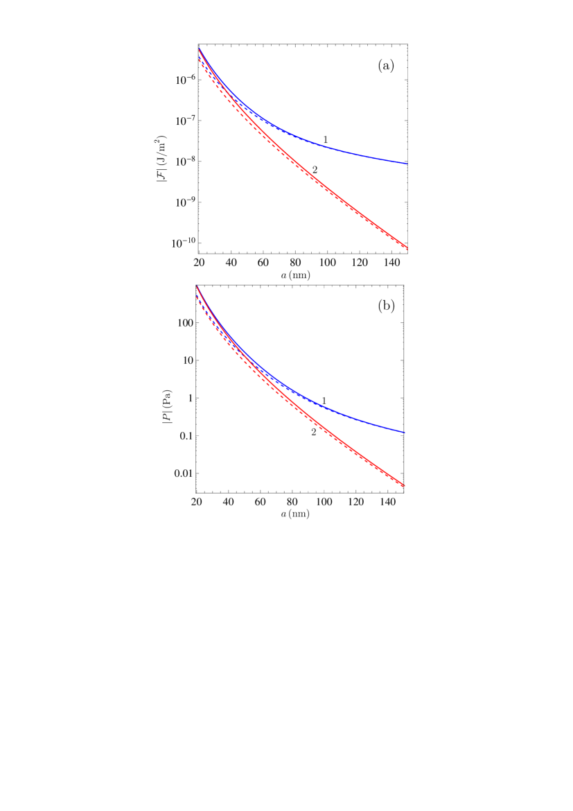
Figure 2: (Color online) The magnitudes of (a) the Casimir free energy per unit area and (b) the Casimir pressure are computed at $T=300\,$K using the Drude model (solid and dashed lines labeled 1) and the plasma model (solid and dashed lines labeled 2) approaches versus the film thickness for a free-standing Ni film in vacuum (solid lines 1 and 2) and for a Ni film sandwiched between two sapphire plates (dashed lines 1 and 2).

In Fig. 2(a) the computational results for the magnitude of the (negative) Casimir free energy of Ni film in vacuum are shown by the pair of solid lines 1 and 2 as the functions of film thickness computed using the Drude and plasma model approaches, respectively. The dashed lines 1 and 2 present similar results for the configuration of Ni film sandwiched between two sapphire plates. As is seen in Fig. 2(a), in both configurations the free energies computed using the Drude model approach (the solid and dashed lines labeled 1) go to the common classical limit (12) which is already reached for a film of 150 nm thickness. This corresponds to the characteristic frequency $c/a\approx 1.3\,$eV which is much larger than the relaxation parameter for Ni (see Sec. II). One can conclude that the classical limit is reached in the frequency region of infrared optics where the skin depth of a Drude model is equal to $\delta=c/\omega_{p,{\rm Ni}}\approx 40\,$nm. If the plasma model approach is used (the solid and dashed lines labeled 2) the Casimir free energy in both configurations drops to zero exponentially fast.

From Fig. 2(a) it is seen that for Ni films of several tens of nanometers thickness the Drude model approach predicts considerably larger magnitudes of the Casimir free energy than the plasma model one. Thus, for the Ni films of 50 and 100 nm thickness in vacuum (see the solid lines 1 and 2) this excess is by the factors of 1.63 and 9.95, respectively. Recall that for the configuration of two metallic plates separated with a vacuum gap of width $a$ the theoretical predictions of both approaches at $a<1\,\mu$m differ by only a few percent. By the factor of two difference is achieved only at $a\approx 6\,\mu$m. For the Ni films of 50 and 100 nm thickness sandwiched between two sapphire plates (see the dashed lines 1 and 2) the magnitudes of the Casimir free energy predicted by the Drude and plasma model approaches differ by the factors of 1.84 and 11.47, respectively. Note that for the configuration of a Ni film deposited on a sapphire plate (the second sapphire plate is replaced with a vacuum) the Casimir free energy of a film is sandwiched between the free energies computed for the two configurations considered above [see Fig. 2(a)].

In Fig. 2(b) we present the computational results for the magnitudes of the (negative) Casimir pressure of Ni film as the functions of film thickness. As in Fig. 2(a), the solid lines labeled 1 and 2 are computed using the Drude and plasma model approaches, respectively, for the configuration of a free-standing Ni film in vacuum. The dashed lines 1 and 2 present similar results for a Ni film sandwiched between two sapphire plates. As is seen in Fig. 2(b), the Casimir pressure of the magnetic film possesses the same characteristic properties, as the Casimir free energy. It is of most importance that the theoretical predictions of both theoretical approaches differ significantly for already thin magnetic films and that the Casimir pressures computed using the Drude model approach (the solid and dashed lines 1) go to the classical limit (13), whereas the same pressure computed using the plasma model approach drops to zero exponentially fast (see the solid and dashed lines 2).

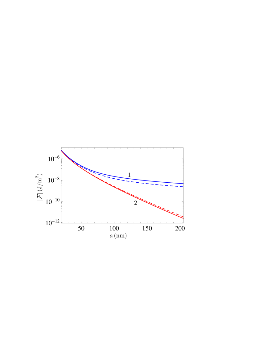
Figure 3: (Color online) The magnitudes of the Casimir free energy per unit area of the free-standing in vacuum Ni (solid lines) and Pt (dashed lines) films are computed at $T=300\,$K versus the film thickness using the Drude model (solid and dashed lines labeled 1) and the plasma model (solid and dashed lines labeled 2) approaches.

It is interesting to compare the Casimir free energy of a Ni film and a film made of some nonmagnetic metal, e.g., of Pt, which plasma frequency is approximately equal to that of Ni. The dielectric permittivity of Pt along the imaginary frequency axis is given in Sec. II. In Fig. 3 the computational results for the magnitudes of the (negative) Casimir free energy of the free-standing in vacuum Ni (the two solid lines) and Pt (the two dashed lines) films are shown as the functions of film thickness. The pairs of solid and dashed lines labeled 1 and 2 are computed using the Drude and plasma model approaches, respectively. As is seen in Fig. 3, there is a difference by a factor of two in the classical limits for the free energies of Ni and Pt films which are already reached at $a=200\,$nm. This is because the classical limit for the solid line 1 (Ni) is given by Eq. (12), whereas the classical limit for the dashed line 1 (Pt) is given by 47

$${\cal F}_{\rm Pt}^{(l=0)}(a,T)=-\frac{k_{B}T}{16\pi a^{2}}\zeta(3).$$ (22)

When the plasma model approach is used in computations (the dashed and solid lines labeled 2), the Casimir free energy of both nonmagnetic and magnetic films exponentially fast drops to zero with increasing film thickness.

IV Magnetic film deposited on nonmagnetic metal

In this section we consider a Ni film of thickness $a$ deposited on thick metallic plates made of either Cu or Al. The role of the third body is now played by a vacuum. In mathematical expressions below we use the index Cu as an indication of the plate material, but it can be replaced with Al or any other metal. We start with the contributions of the zero-frequency terms to the Casimir free energy and pressure calculated using the Drude model approach. Then from Eq. (2) one obtains

$$r_{{\rm TM},D}^{(2,3)}(0,k_{\bot})=-1,$$

$$r_{{\rm TM},D}^{(2,1)}(0,k_{\bot})=\frac{\omega_{p,{\rm Cu}}^{2}\gamma_{\rm Ni}-\omega_{p,{\rm Ni}}^{2}\gamma_{\rm Cu}}{\omega_{p,{\rm Cu}}^{2}\gamma_{\rm Ni}+\omega_{p,{\rm Ni}}^{2}\gamma_{\rm Cu}}\equiv R_{0,{\rm NiCu}},$$

$$r_{{\rm TE},D}^{(2,n)}(0,k_{\bot})=r_{0,{\rm Ni}},$$ (23)

where $r_{0,{\rm Ni}}$ is defined in Eq. (9).

Substituting Eq. (23) in Eq. (1) and using the dimensionless variable $y=2ak_{\bot}$, we find

$${\cal F}_{D}^{(l=0)}(a,T)=\frac{k_{B}T}{16\pi a^{2}}\int_{0}^{\infty}ydy$$ (24)

$$~{}\times\left[\ln(1+R_{0,{\rm NiCu}}e^{-y})+\ln(1-r_{0,{\rm Ni}}^{2}e^{-y})\right].$$

After the integration this results in

$${\cal F}_{D}^{(l=0)}(a,T)=-\frac{k_{B}T}{16\pi a^{2}}\left[{\rm Li}_{3}(-R_{0,{\rm NiCu}})+{\rm Li}_{3}(r_{0,{\rm Ni}}^{2})\right].$$ (25)

In a similar way, for the Casimir pressure (8) one arrives at

$${P}_{D}^{(l=0)}(a,T)=-\frac{k_{B}T}{16\pi a^{3}}\int_{0}^{\infty}y^{2}dy$$ (26)

$$~{}\times\left[-(R_{0,{\rm NiCu}}^{-1}e^{y}+1)^{-1}+(r_{0,{\rm Ni}}^{-2}e^{y}-1)^{-1}\right]$$

$$~{}=-\frac{k_{B}T}{8\pi a^{3}}\left[{\rm Li}_{3}(-R_{0,{\rm NiCu}})+{\rm Li}_{3}(r_{0,{\rm Ni}}^{2})\right].$$

Taking into account the parameters of our configuration, we find from Eqs. (9) and (23) that $r_{0,{\rm Ni}}=-0.9820$ and $R_{0,{\rm NiCu}}=0.6116$. This results in

$${\rm Li}_{3}(-R_{0,{\rm NiCu}})=-0.5716,\quad{\rm Li}_{3}(r_{0,{\rm Ni}}^{2})=1.1454,$$ (27)

i.e., the zero-frequency terms (25) and (26) are negative [note that respective contributions to Eqs. (12) and (13) have similar signs]. As is seen from the results of numerical computations below, ${\cal F}_{D}^{(l\geq 1)}(a,T)>0$ and for small film thicknesses it holds

$$|{\cal F}_{D}^{(l\geq 1)}(a,T)|>|{\cal F}_{D}^{(l=0)}(a,T)|.$$ (28)

Because of this, the free energy of a Ni film deposited on a nonmagnetic metal plate changes its sign with increasing film thickness if the Drude model approach is used in computations (see below for the values of $a$, where the Casimir free energy and pressure change sign, for specific plate metals). Note that this change of sign is not of the same nature, as for some liquid-separated plates (see, e.g., Refs. 2 ; 64a ). In our case the effect is caused by the influence of magnetic properties on the zero-frequency term when the Drude model is used in calculations.

Now we calculate the zero-frequency contribution to the free energy and pressure of a Ni film deposited on a Cu plate using the plasma model. From Eq. (2) for the TM reflection coefficients we find

$$r_{{\rm TM},p}^{(2,3)}(0,k_{\bot})=-1,$$ (29)

$$r_{{\rm TM},p}^{(2,1)}(0,k_{\bot})=\frac{\omega_{p,{\rm Cu}}^{2}\sqrt{c^{2}k_{\bot}^{2}+\mu_{\rm Ni}\omega_{p,{\rm Ni}}^{2}}-\omega_{p,{\rm Ni}}^{2}\sqrt{c^{2}k_{\bot}^{2}+\omega_{p,{\rm Cu}}^{2}}}{\omega_{p,{\rm Cu}}^{2}\sqrt{c^{2}k_{\bot}^{2}+\mu_{\rm Ni}\omega_{p,{\rm Ni}}^{2}}+\omega_{p,{\rm Ni}}^{2}\sqrt{c^{2}k_{\bot}^{2}+\omega_{p,{\rm Cu}}^{2}}}.$$

The TE reflection coefficient $r_{{\rm TE},p}^{(2,3)}(0,k_{\bot})=R_{0,{\rm Ni}}(k_{\bot})$ coincides with that given by Eq. (15) with $n=3$. The second TE reflection coefficient is given by

$$r_{{\rm TE},p}^{(2,1)}(0,k_{\bot})=\frac{\sqrt{c^{2}k_{\bot}^{2}+\mu_{\rm Ni}\omega_{p,{\rm Ni}}^{2}}-\mu_{\rm Ni}\sqrt{c^{2}k_{\bot}^{2}+\omega_{p,{\rm Cu}}^{2}}}{\sqrt{c^{2}k_{\bot}^{2}+\mu_{\rm Ni}\omega_{p,{\rm Ni}}^{2}}+\mu_{\rm Ni}\sqrt{c^{2}k_{\bot}^{2}+\omega_{p,{\rm Cu}}^{2}}}.$$ (30)

In terms of the variable $v$ the coefficient $r_{{\rm TE},p}^{(2,3)}$ is given by Eq. (19) and two nontrivial coefficients in Eqs. (29) and (30) take the form

$$r_{{\rm TM},p}^{(2,1)}(0,v)=\frac{\tilde{\omega}_{p,{\rm Cu}}^{2}v-\tilde{\omega}_{p,{\rm Ni}}^{2}\sqrt{v^{2}-\mu_{\rm Ni}\tilde{\omega}_{p,{\rm Ni}}^{2}+\tilde{\omega}_{p,{\rm Cu}}^{2}}}{\tilde{\omega}_{p,{\rm Cu}}^{2}v+\tilde{\omega}_{p,{\rm Ni}}^{2}\sqrt{v^{2}-\mu_{\rm Ni}\tilde{\omega}_{p,{\rm Ni}}^{2}+\tilde{\omega}_{p,{\rm Cu}}^{2}}}\equiv R_{0,{\rm TM}}(v),$$

(31)

$$r_{{\rm TE},p}^{(2,1)}(0,v)=\frac{v-\mu_{\rm Ni}\sqrt{v^{2}-\mu_{\rm Ni}\tilde{\omega}_{p,{\rm Ni}}^{2}+\tilde{\omega}_{p,{\rm Cu}}^{2}}}{v+\mu_{\rm Ni}\sqrt{v^{2}-\mu_{\rm Ni}\tilde{\omega}_{p,{\rm Ni}}^{2}+\tilde{\omega}_{p,{\rm Cu}}^{2}}}\equiv R_{0,{\rm TE}}(v).$$

As a result, the zero-frequency contribution to the Casimir free energy can be written as

$${\cal F}_{p}^{(l=0)}(a,T)=\frac{k_{B}T}{16\pi a^{2}}\int_{\sqrt{\mu_{\rm Ni}}\tilde{\omega}_{p,{\rm Ni}}}^{\infty}vdv$$ (32)

$$\times\left[\ln(1+R_{0,{\rm TM}}(v)e^{-v})+\ln(1-R_{0,{\rm Ni}}(v)R_{0,{\rm TE}}(v)e^{-v})\right].$$

The zero-frequency contribution to the Casimir pressure is the following:

$${P}_{p}^{(l=0)}(a,T)=-\frac{k_{B}T}{16\pi a^{3}}\int_{\sqrt{\mu_{\rm Ni}}\tilde{\omega}_{p,{\rm Ni}}}^{\infty}v^{2}dv$$ (33)

$$\times\left\{-\left[R_{0,{\rm TM}}^{-1}(v)e^{v}+1\right]^{-1}+\left[R_{0,{\rm Ni}}^{-1}(v)R_{0,{\rm TE}}^{-1}(v)e^{v}-1\right]^{-1}\right\}.$$

Numerical computations and the analysis performed in Ref. 47 show that in the framework of the plasma model approach

$$|{\cal F}_{p}^{(l=0)}(a,T)|\ll|{\cal F}_{p}^{(l\geq 1)}(a,T)|$$ (34)

for any film thickness. Similar to the case of the Drude model, it holds ${\cal F}_{p}^{(l\geq 1)}(a,T)>0$. However, unlike the Drude model, here the sign of ${\cal F}_{p}^{(l\geq 1)}$ determines the positive sign (i.e., the repulsive character) of the total Casimir free energy of a magnetic film.

In Fig. 4(a) we present the computational results for the magnitudes of the Casimir free energy of Ni films deposited on Cu and Al plates computed as functions of film thickness using the Drude model (lines labeled 1) and plasma model (lines labeled 2) approaches. In Fig. 4(b) similar results are presented for the Casimir pressure of Ni films. As is seen from Fig. 4(a,b), the Casimir free energy and pressure of a Ni film calculated using the Drude model approach vanish at some film thickness and then change their sign. At film thickness of approximately 150 nm both quantities reach their classical limits (25) and (26). For the case of Cu plate the Casimir free energy and pressure are positive for films thinner than 61.1 and 83.3 nm, respectively. For the films of these thicknesses the Casimir free energy and pressure vanish and become negative for thicker films. In the case of an Al plate, the Casimir free energy and pressure calculated using the Drude model approach take zero value for $a=77.9$ and 102.7 nm, respectively. In the limiting case of $\omega_{p,{\rm Ni}}\to\infty$ (the limit of ideal metal) we have from Eq. (23) $R_{0,{\rm NiCu}}\to-1$ and Eq. (25) transforms to Eq. (13) taking into account that ${\rm Li}_{3}(1)=\zeta(3)$. This is a nonzero free energy of an ideal metal film, i.e., a counter intuitive result, as discussed above.

According to Fig. 4(a,b), quite different results are obtained when the plasma model approach is used in computations (lines labeled 2). In this case the Casimir free energy and pressure of Ni films are positive (i.e., correspond to repulsion) and drop exponentially fast to zero with increasing film thickness. The classical limit is not reached for films of any thickness. An important point is that theoretical predictions for the magnitudes of the Casimir free energy and pressure using the Drude and plasma model approaches are significantly different even for relatively thin Ni films. Thus, for Ni films of 50, 60, and 100 nm thickness deposited on a Cu plate the magnitudes of the Casimir free energies computed using both approaches differ by the factors of 2.44, 140.66 and 6.88, respectively. For Ni films of 50, 75, and 100 nm thickness deposited on an Al plate the respective factors are 1.26, 8.98, and 2.56. It is seen that the major difference in theoretical predictions of the Drude and plasma model approaches occurs for film thicknesses where the Drude model prediction is close to zero. Similar results are obtained for the Casimir pressure.

Now we investigate in more detail why the Casimir free energy and pressure change sign as functions of film thickness if the Drude model approach is used in computations. For this purpose, the solid line in Fig. 5 shows the quantity $a^{2}{\cal F}_{D}$ for a Ni film deposited on a Cu plate as a function of film thickness $a$. It is seen that the free energy changes its sign from positive to negative in accordance with Fig. 4(a). In the same figure the dotted line shows the zero-frequency contribution (32) to the Casimir free energy, which is a negative quantity. The dashed-dotted line in Fig. 5 presents the contribution of all Matsubara terms with nonzero frequencies to $a^{2}{\cal F}_{D}$, which is positive for the pair of metals Ni and Cu under consideration. As a result, the free energy ${\cal F}_{D}$ of a Ni film is positive for sufficiently thin films and becomes negative with increasing film thickness.

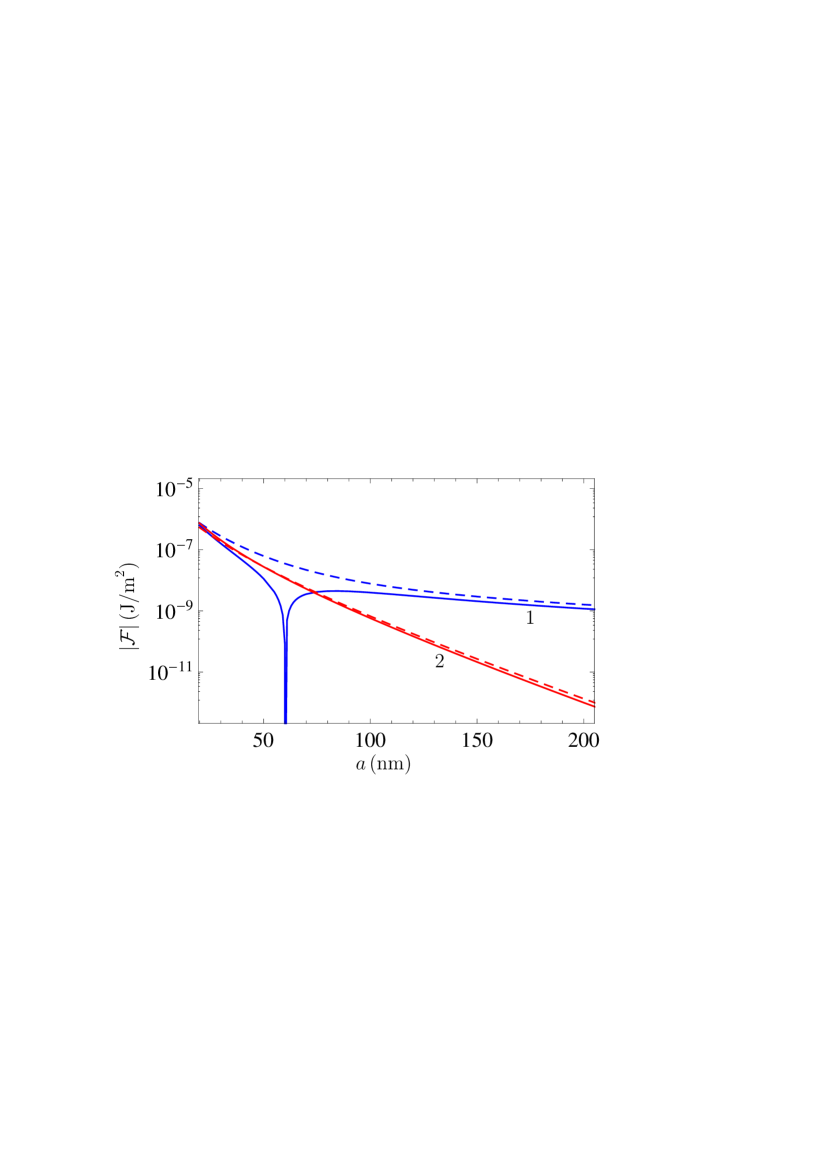
Figure 6: (Color online) The magnitudes of the Casimir free energy per unit area are computed at $T=300\,$K using the Drude model (solid and dashed lines labeled 1) and the plasma model (solid and dashed lines labeled 2) approaches versus the film thickness for a Ni film (solid lines 1 and 2) and for a Pt film (dashed lines 1 and 2) deposited on Cu plates. The Casimir interaction of Pt film is repulsive for both the plasma and Drude models.

Next, we consider the role of magnetic properties of the film in the effects discussed above. For this purpose, in Fig. 6 we reproduce from Fig. 4 the magnitudes of the Casimir free energy of a Ni film deposited on a Cu plate computed using the Drude and plasma model approaches (solid lines 1 and 2, respectively). In the same figure the dashed lines 1 and 2 show the Casimir free energy of a nonmagnetic Pt film deposited on a Cu plate and computed using the two approaches. These computations were performed using the dielectric permittivity of Pt presented on an inset to Fig. 1(a). The zero-frequency reflection coefficients are given by Eqs. (19) and (31) where $\mu_{\rm Ni}$ and $\omega_{p,{\rm Ni}}$ are replaced with unity and $\omega_{p,{\rm Pt}}$, respectively. As is seen in Fig. 6, the solid and dashed lines labeled 2 are similar in appearance, i.e., the magnetic properties of a film influence the Casimir free energy computed using the plasma model approach only quantitatively (note that for both films ${\cal F}_{P}>0$). If, however, the Drude model approach is used, this leads to fundamental differences between the Casimir free energies of nonmagnetic and magnetic films. Thus, the solid line 1 demonstrates the Casimir free energy of a magnetic Ni film which changes its sign from positive to negative and takes the zero value for the film of some definite thickness (see above). At the same time, the Casimir free energy of a nonmagnetic Pt film (the dashed line 1) is positive for any film thickness. This is also seen from the classical limit for a Pt film deposited on a Cu plate which is positive

$${\cal F}_{\rm Pt}^{(l=0)}(a,T)=-\frac{k_{B}T}{16\pi a^{2}}{\rm Li}_{3}(-R_{0,{\rm PtCu}})>0,$$ (35)

where $R_{0,{\rm PtCu}}$ is defined by Eq. (23) with the index Ni replaced for Pt. As a result, the use of magnetic films presents additional possibilities for discrimination between the Drude and plasma model approaches in the Lifshitz theory.

V Magnetic film deposited on magnetic metal

In this section we calculate the Casimir free energy and pressure of a magnetic Ni film deposited on a plate made of magnetic metal. Numerical computations are performed for a Fe plate using both the Drude and plasma model approaches. We begin with the Drude model approach. In this case the reflection coefficients $r_{{\rm TM},D}^{(2,n)}$ at zero Matsubara frequency are again given by the first two lines of Eq. (23) where the index Cu is replaced with Fe. The reflection coefficient $r_{{\rm TE},D}^{(2,3)}$ at zero frequency is given by the third line of Eq. (23), whereas the coefficient $r_{{\rm TE},D}^{(2,1)}$ is given by

$$r_{{\rm TE},D}^{(2,1)}(0,k_{\bot})=\frac{\mu_{\rm Fe}-\mu_{\rm Ni}}{\mu_{\rm Fe}+\mu_{\rm Ni}}\equiv r_{0,{\rm NiFe}}>0.$$ (36)

As a result, the zero-frequency contribution to the Casimir free energy of a Ni film on a Fe plate, calculated using the Drude model, takes the form

$${\cal F}_{D}^{(l=0)}(a,T)=\frac{k_{B}T}{16\pi a^{2}}\int_{0}^{\infty}ydy$$ (37)

$$~{}\times\left[\ln(1+R_{0,{\rm NiFe}}e^{-y})+\ln(1-r_{0,{\rm Ni}}r_{0,{\rm NiFe}}e^{-y})\right].$$

Note that $r_{0,{\rm Ni}}r_{0,{\rm NiFe}}<0$. As a result, ${\cal F}_{D}^{(l=0)}>0$, as opposed to the case of nonmagnetic plate considered in Sec. IV. As is seen from the results of numerical computations (see below), the contribution of all Matsubara terms with nonzero frequency, ${\cal F}_{D}^{(l\geq 1)}$, changes its sign from plus to minus with increasing film thickness, leaving the total free energy ${\cal F}_{D}$ positive. After the integration in Eq. (37), one obtains the classical limit

$${\cal F}_{D}^{(l=0)}(a,T)=-\frac{k_{B}T}{16\pi a^{2}}\left[{\rm Li}_{3}(-R_{0,{\rm NiFe}})+{\rm Li}_{3}(r_{0,{\rm Ni}}r_{0,{\rm NiFe}})\right].$$ (38)

In a similar way, for the zero-frequency contribution to the Casimir pressure of a Ni film on a Fe plate we find

$${P}_{D}^{(l=0)}(a,T)=-\frac{k_{B}T}{16\pi a^{3}}\int_{0}^{\infty}y^{2}dy$$ (39)

$$~{}\times\left[-(R_{0,{\rm NiFe}}^{-1}e^{y}+1)^{-1}+(r_{0,{\rm Ni}}^{-1}r_{0,{\rm NiFe}}^{-1}e^{y}-1)^{-1}\right]$$

$$~{}=-\frac{k_{B}T}{8\pi a^{3}}\left[{\rm Li}_{3}(-R_{0,{\rm NiFe}})+{\rm Li}_{3}(r_{0,{\rm Ni}}r_{0,{\rm NiFe}})\right]>0.$$

We continue by considering the same configuration using the plasma model approach. In this case the reflection coefficient $r_{{\rm TM},p}^{(2,3)}$ is given by the first line of Eq. (29) and the coefficient $r_{{\rm TM},p}^{(2,1)}$ is given by

$$r_{{\rm TM},p}^{(2,1)}(0,k_{\bot})=\frac{\omega_{p,{\rm Fe}}^{2}\sqrt{c^{2}k_{\bot}^{2}+\mu_{\rm Ni}\omega_{p,{\rm Ni}}^{2}}-\omega_{p,{\rm Ni}}^{2}\sqrt{c^{2}k_{\bot}^{2}+\mu_{\rm Fe}\omega_{p,{\rm Fe}}^{2}}}{\omega_{p,{\rm Fe}}^{2}\sqrt{c^{2}k_{\bot}^{2}+\mu_{\rm Ni}\omega_{p,{\rm Ni}}^{2}}+\omega_{p,{\rm Ni}}^{2}\sqrt{c^{2}k_{\bot}^{2}+\mu_{\rm Fe}\omega_{p,{\rm Fe}}^{2}}}.$$ (40)

As to TE reflection coefficients at zero Matsubara frequency, $r_{{\rm TE},p}^{(2,3)}$ is given by Eq. (15) with $n=3$ and $r_{{\rm TE},p}^{(2,1)}$ takes the form

$$r_{{\rm TE},p}^{(2,1)}(0,k_{\bot})=\frac{\mu_{\rm Fe}\sqrt{c^{2}k_{\bot}^{2}+\mu_{\rm Ni}\omega_{p,{\rm Ni}}^{2}}-\mu_{\rm Ni}\sqrt{c^{2}k_{\bot}^{2}+\mu_{\rm Fe}\omega_{p,{\rm Fe}}^{2}}}{\mu_{\rm Fe}\sqrt{c^{2}k_{\bot}^{2}+\mu_{\rm Ni}\omega_{p,{\rm Ni}}^{2}}+\mu_{\rm Ni}\sqrt{c^{2}k_{\bot}^{2}+\mu_{\rm Fe}\omega_{p,{\rm Fe}}^{2}}}.$$ (41)

In terms of the dimensionless variable $v$ the coefficient $r_{{\rm TE},p}^{(2,3)}$ is given by Eq. (19) and the coefficients (40) and (41) are as follows:

$$r_{{\rm TM},p}^{(2,1)}(0,v)=\frac{\tilde{\omega}_{p,{\rm Fe}}^{2}v-\tilde{\omega}_{p,{\rm Ni}}^{2}\sqrt{v^{2}-\mu_{\rm Ni}\tilde{\omega}_{p,{\rm Ni}}^{2}+\mu_{\rm Fe}\tilde{\omega}_{p,{\rm Fe}}^{2}}}{\tilde{\omega}_{p,{\rm Fe}}^{2}v+\tilde{\omega}_{p,{\rm Ni}}^{2}\sqrt{v^{2}-\mu_{\rm Ni}\tilde{\omega}_{p,{\rm Ni}}^{2}+\mu_{\rm Fe}\tilde{\omega}_{p,{\rm Fe}}^{2}}}\equiv\tilde{R}_{0,{\rm TM}}(v),$$

(42)

$$r_{{\rm TE},p}^{(2,1)}(0,v)=\frac{\mu_{\rm Fe}v-\mu_{\rm Ni}\sqrt{v^{2}-\mu_{\rm Ni}\tilde{\omega}_{p,{\rm Ni}}^{2}+\mu_{\rm Fe}\tilde{\omega}_{p,{\rm Fe}}^{2}}}{\mu_{\rm Fe}v+\mu_{\rm Ni}\sqrt{v^{2}-\mu_{\rm Ni}\tilde{\omega}_{p,{\rm Ni}}^{2}+\mu_{\rm Fe}\tilde{\omega}_{p,{\rm Fe}}^{2}}}\equiv\tilde{R}_{0,{\rm TE}}(v).$$

Then, the zero-frequency contribution to the Casimir free energy and pressure calculated using the plasma model approach are

$${\cal F}_{p}^{(l=0)}(a,T)=\frac{k_{B}T}{16\pi a^{2}}\int_{\sqrt{\mu_{\rm Ni}}\tilde{\omega}_{p,{\rm Ni}}}^{\infty}vdv$$

$$\times\left[\ln(1+\tilde{R}_{0,{\rm TM}}(v)e^{-v})+\ln(1-R_{0,{\rm Ni}}(v)\tilde{R}_{0,{\rm TE}}(v)e^{-v})\right],$$

$${P}_{p}^{(l=0)}(a,T)=-\frac{k_{B}T}{16\pi a^{3}}\int_{\sqrt{\mu_{\rm Ni}}\tilde{\omega}_{p,{\rm Ni}}}^{\infty}v^{2}dv$$ (43)

$$\times\left\{-\left[\tilde{R}_{0,{\rm TM}}^{-1}(v)e^{v}+1\right]^{-1}+\left[R_{0,{\rm Ni}}^{-1}(v)\tilde{R}_{0,{\rm TE}}^{-1}(v)e^{v}-1\right]^{-1}\right\}.$$

According to the results of Ref. 47 obtained for nonmagnetic metals,

$$|{\cal F}_{p}^{(l=0)}(a,T)|\ll|{\cal F}_{p}^{(l\geq 1)}(a,T)|$$ (44)

for any film thickness $a$. Taking into account that the magnetic properties only decrease the magnitude of the zero-frequency terms, Eq. (44) is also valid for our case of magnetic metals.

Numerical computations of the Casimir free energy and pressure for a Ni film deposited on a Fe plate were performed using the Drude and plasma model approaches with the dielectric permittivity of Fe along the imaginary frequency axis presented in Fig. 1(b). In Fig. 7(a) we present the computational results for the magnitude of the Casimir free energy as a function of film thickness computed using the Drude model (line 1) and plasma model (line 2) approaches. As is seen in Fig. 7(a), the free energy ${\cal F}_{D}$ goes to its classical limit (39), whereas the free energy ${\cal F}_{p}$ exponentially fast drops to zero. The free energy ${\cal F}_{D}$ is positive for all $a$, and the free energy ${\cal F}_{p}$ is positive for sufficiently thin films, takes zero value for the film of 46.95 nm thickness and becomes negative for thicker films. This is just the opposite to Figs. 4(a) and 6, where the Casimir free energy computed using the Drude model approach changes its sign, whereas the one calculated using the plasma model remains positive.

The next important feature of Fig. 7 is that the differences in theoretical predictions of the Drude and plasma models are much larger than for a plate made of nonmagnetic metal. Thus, for Ni films of 47, 50, and 100 nm thickness the magnitudes of the Casimir free energy predicted using both theoretical approaches are different by the factors of 5866, 133.3, and 142.0, respectively. The largest difference for a film of 47 nm thickness is explained by the fact that for a film of 46.95 nm thickness ${\cal F}_{p}=0$.

The computational results for the magnitudes of the Casimir pressure are presented in Fig. 7(b) by the line 1 (the Drude model approach) and line 2 (the plasma model approach) as the functions of film thickness. The line 1 corresponds to the Casimir repulsion and follows the classical limit (39) for Ni films of more than 150 nm thickness. The line 2 describes the Casimir repulsion for the films of less than 57.4 nm thickness, where the Casimir pressure computed using the plasma model takes zero value. For the films of larger thickness the Casimir pressure $P_{p}$ takes negative values and drops to zero exponentially fast. In Fig. 7(b) the differences in the Casimir pressures predicted by the Drude and plasma model approaches are much larger than those in Figs. 2(b) and 4(b). Because of this, the magnetic plate is advantageous for making discrimination between the two approaches.

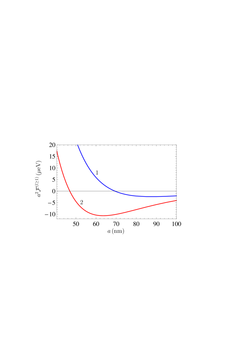
Figure 8: (Color online) The contribution of all nonzero Matsubara frequencies to the Casimir free energy per unit area of a Ni film deposited on a Fe plate is computed at $T=300\,$K using the Drude model (line 1) and the plasma model (line 2) approaches versus the film thickness.

Now we illustrate the role of the Matsubara terms with nonzero frequencies in the complete Casimir free energies in Fig. 7(a) computed using the Drude and plasma model approaches. In Fig. 8 we present the computational results for the quantity $a^{2}{\cal F}^{(l\geq 1)}(a,T)$ computed using the Drude model (line 1) and plasma model (line 2) approaches as the functions of film thickness. As is seen in Fig. 8, the contribution of all nonzero Matsubara frequencies changes its sign for both theoretical approaches. In the case of the Drude model approach, however, the contribution of the zero-frequency term (38) remains much larger in magnitude: $a^{2}{\cal F}_{D}^{(l=0)}(a,T)=575.6\,\mu$eV. This explains why the total free energy computed using the Drude model approach remains positive for Ni films of any film thickness. If the plasma model approach is used (line 2), the contribution of the zero-frequency Matsubara term is negligibly small in accordance to Eq. (44). This is the reason why the complete Casimir free energy ${\cal F}_{p}(a,T)$ changes its sign with increasing film thickness.

VI Conclusions and discussion

In the foregoing we have calculated the Casimir free energy and pressure for a magnetic metal film (Ni) sandwiched between two dielectric plates (sapphire) or deposited on a plate made of either nonmagnetic (Cu, Al) or magnetic (Fe) metal. All calculations have been performed at room temperature using the tabulated optical data of all metals under consideration in the framework of both the Drude and plasma model approaches to the Lifshitz theory of the van der Waals and Casimir forces. This is important in connection with the problem in Casimir physics concerning the role of dissipation of free charge carriers discussed in Sec. I.

According to our results, the Casimir free energy and pressure of magnetic films differ widely depending on the calculation approach used for already rather thin films. For the free-standing, sandwiched between two sapphire plates or deposited on Cu and Al plates Ni films of several tens nanometer thickness these differences reach hundreds and thousands percent. For a Ni film of 47 nm thickness deposited on a plate made of magnetic metal (Fe) the Casimir free energies predicted using the Drude and plasma approaches differ by the factor of 5866. This opens opportunities for an unambiguous experimental discrimination between the two approaches with no resort to the differential force measurements.

We have shown that the Casimir free energy and pressure of a magnetic film calculated using the Drude model approach possess the classical limit in all configurations considered above, which is reached at about 150 nm film thickness. If the plasma model approach is used in calculations, the Casimir free energy and pressure have no classical limit, but, instead, exponentially fast drop to zero with increasing film thickness. The absence of the classical limit, however, is not a disadvantage of the plasma model approach, but more likely is its merit. The point is that for a metallic film the presence of the classical limit results in a nonzero Casimir free energy even though the metal of a film becomes an ideal one. This result should be considered as an indication of failure because the fluctuating electromagnetic filed cannot penetrate in an interior of ideal metal. The reason for so strong influence of magnetic properties when the Drude model approach is used is that they act only through the zero-frequency term of the Lifshitz formula. The latter is dominant in the Drude model approach and negligibly small in the plasma model one, as compared to the contribution of all nonzero Matsubara frequencies.

The numerical computations show that if the Drude model approach is used the Casimir free energy and pressure of a Ni film deposited on nonmagnetic plates made of Cu and Al change their sign with increasing film thickness. In the framework of the plasma model approach these quantities are positive for all film thicknesses, i.e., correspond to the Casimir repulsion. The situation changes if a Ni film is deposited on a magnetic Fe plate. In this case the Casimir free energy and pressure are positive if the Drude model approach is used and change their sign with increasing film thickness if calculations are performed using the plasma model approach. All these results are important not only for the discrimination between existing theoretical approaches, but also in the investigation of stability of thin films.

The possibility to directly measure the single-film Casimir pressure is discussed in Ref. 47 . For this purpose, the most often used sphere-plate geometry can be employed, where the solid metallic film is replaced with a liquid metal like mercury or, more conveniently, with an alloy of gallium and indium. In our case the magnetic liquid metals should be used 61 . The predicted effects can be also observed in the Casimir chips 19 , where it is not difficult to maintain parallelity. In this case the Casimir pressure in a magnetic film is measurable by means of an additional piezo sensor.

An answer to the question why the plasma model approach to the Casimir force is consistent with experimental data and thermodynamics though the plasma model does not describe the optical properties and conductivity of metals at low frequencies might be rooted in the foundations of quantum statistical physics. The optical properties and conductivity of metals are measured as a response of a system to the electromagnetic fields with nonzero expectation values. The usually used postulate that the dielectric response of metals to the fluctuating fields having a zero expectation value is precisely the same is some kind of extrapolation, which works good in classical statistical physics, but might be not applicable to all kinds of low-frequency quantum fluctuations. Future investigation will show whether this approach is helpful for the resolution of the problems in Casimir physics.

Figure 1: The dielectric permittivities of (a) Ni and Pt (the inset) and (b) Al, Cu, and Fe are shown as functions of the imaginary frequency normalized to the first Matsubara frequency by the pairs of upper and lower lines obtained through extrapolations of the optical data using the plasma and Drude models, respectively.

                 

         

Figure 4: (Color online) The magnitudes of (a) the Casimir free energy per unit area and (b) the Casimir pressure are computed at $T=300\,$K using the Drude model (lines labeled 1) and the plasma model (lines labeled 2) approaches versus the film thickness for a Ni film deposited on Cu and Al plates. If the plasma model is used, the Casimir interaction is repulsive. In the case of the Drude model, repulsion at short separations changes for attraction at larger separations.

         

Figure 5: (Color online) The Casimir free energy per unit area of a Ni film deposited on a Cu plate is computed at $T=300\,$K using the Drude model approach (solid line) versus the film thickness. The dotted and dashed-dotted lines show contributions to the free energy of the zero-frequency term and all terms with nonzero Matsubara frequencies, respectively.

         

         

Figure 7: (Color online) The magnitudes of (a) the Casimir free energy per unit area and (b) the Casimir pressure are computed at $T=300\,$K using the Drude model (lines labeled 1) and the plasma model (lines labeled 2) approaches versus the film thickness for a Ni film deposited on a Fe plate. If the plasma model is used, the Casimir interaction is repulsive at short separations and attractive at larger separations. In the case of the Drude model, the Casimir interaction is repulsive.

References

- (1) V. A. Parsegian, Van der Waals Forces: A Handbook for Biologists, Chemists, Engineers, and Physicists (Cambridge University Press, Cambridge, 2005).
- (2) M. Bordag, G. L. Klimchitskaya, U. Mohideen, and V. M. Mostepanenko, Advances in the Casimir Effect (Oxford University Press, Oxford, 2015).
- (3) J. F. Babb, G. L. Klimchitskaya, and V. M. Mostepanenko, Phys. Rev. A 70, 042901 (2004).
- (4) M. Antezza, L. P. Pitaevskii, and S. Stringari, Phys. Rev. A 70, 053619 (2004).
- (5) A. O. Caride, G. L. Klimchitskaya, V. M. Mostepanenko, and S. I. Zanette, Phys. Rev. A 71, 042901 (2005).
- (6) S. Y. Buhmann and S. Scheel, Phys. Rev. Lett. 100, 253201 (2008).
- (7) H. Safari, D.-G. Welsch, S. Y. Buhmann, and S. Scheel. Phys. Rev. A 78, 062901 (2008).
- (8) M. Chaichian, G. L. Klimchitskaya, V. M. Mostepanenko, and A. Tureanu, Phys. Rev. A 86, 012515 (2012).
- (9) F. Chen, G. L. Klimchitskaya, U. Mohideen, and V. M. Mostepanenko, Phys. Rev. Lett. 90, 160404 (2003).
- (10) F. Chen, G. L. Klimchitskaya, V. M. Mostepanenko, and U. Mohideen, Phys. Rev. Lett. 97, 170402 (2006).
- (11) P. J. van Zwol, G. Palasantzas, and J. Th. M. De Hosson, Phys. Rev. B 77, 075412 (2008).
- (12) G. Gómez-Santos, Phys. Rev. B 80, 245424 (2009).
- (13) S. de Man, K. Heeck, and D. Iannuzzi, Phys. Rev. A 82, 062512 (2010).
- (14) D. Drosdoff and L. M. Woods, Phys. Rev. A 84, 062501 (2011).
- (15) H. B. Chan, V. A. Aksyuk, R. N. Kleiman, D. J. Bishop, and F. Capasso, Science 291, 1941 (2001).
- (16) E. Buks and M. L. Roukes, Phys. Rev. B 63, 033402 (2001).
- (17) R. H. French, V. A. Parsegian, R. Podgornik, et al., Rev. Mod. Phys. 82, 1887 (2010).
- (18) R. Esquivel-Sirvent and R. Pérez-Pascual, Eur. Phys. J. B 86, 467 (2013).
- (19) J. Zou, Z. Marcet, A. W. Rodriguez, M. T. H. Reid, A. P. McCauley, I. I. Kravchenko, T. Lu, Y. Bao, S. G. Johnson, and H. B. Chan, Nature Commun. 4, 1845 (2013).
- (20) V. M. Mostepanenko and G. L. Klimchitskaya, Int. J. Mod. Phys. A 25, 2302 (2010).
- (21) V. B. Bezerra, G. L. Klimchitskaya, and V. M. Mostepanenko, Phys. Rev. A 65, 052113 (2002).
- (22) V. B. Bezerra, G. L. Klimchitskaya, and V. M. Mostepanenko, Phys. Rev. A 66, 062112 (2002).
- (23) V. B. Bezerra, G. L. Klimchitskaya, V. M. Mostepanenko, and C. Romero, Phys. Rev. A 69, 022119 (2004).
- (24) M. Bordag and I. Pirozhenko, Phys. Rev. D 82, 125016 (2010).
- (25) G. L. Klimchitskaya and C. C. Korikov, Phys. Rev. A 91, 032119 (2015); 92, 029902(E) (2015).
- (26) V. B. Svetovoy and R. Esquivel, Phys. Rev. E 72, 036113 (2005).
- (27) B. Geyer, G. L. Klimchitskaya, and V. M. Mostepanenko, Phys. Rev. A 70, 422901 (2004).
- (28) R. S. Decca, E. Fischbach, G. L. Klimchitskaya, D. E. Krause, D. López, and V. M. Mostepanenko, Phys. Rev. D 68, 116003 (2003).
- (29) R. S. Decca, D. López, E. Fischbach, G. L. Klimchitskaya, D. E. Krause, and V. M. Mostepanenko, Ann. Phys. (N.Y.) 318, 37 (2005).
- (30) R. S. Decca, D. López, E. Fischbach, G. L. Klimchitskaya, D. E. Krause, and V. M. Mostepanenko, Phys. Rev. D 75, 077101 (2007).
- (31) R. S. Decca, D. López, E. Fischbach, G. L. Klimchitskaya, D. E. Krause, and V. M. Mostepanenko, Eur. Phys. J. C 51, 963 (2007).
- (32) C.-C. Chang, A. A. Banishev, R. Castillo-Garza, G. L. Klimchitskaya, V. M. Mostepanenko, and U. Mohideen, Phys. Rev. B 85, 165443 (2012).
- (33) A. A. Banishev, G. L. Klimchitskaya, V. M. Mostepanenko, and U. Mohideen, Phys. Rev. Lett. 110, 137401 (2013).
- (34) A. A. Banishev, G. L. Klimchitskaya, V. M. Mostepanenko, and U. Mohideen, Phys. Rev. B 88, 155410 (2013).
- (35) V. M. Mostepanenko, J. Phys.: Condens. Matter 27, 214013 (2015).
- (36) S. V. Vonsovskii, Magnetism (J. Wiley, New York, 1974).
- (37) B. Geyer, G. L. Klimchitskaya, and V. M. Mostepanenko, Phys. Rev. B 81, 104101 (2010).
- (38) G. Bimonte, Phys. Rev. Lett. 112, 240401 (2014).
- (39) G. Bimonte, Phys. Rev. Lett. 113, 240405 (2014).
- (40) G. Bimonte, Phys. Rev. B 91, 205443 (2015).
- (41) G. Bimonte, D. López, and R. S. Decca, Phys. Rev. B 93, 184434 (2016).
- (42) R. S. Decca, Int. J. Mod. Phys. A 31, 1641024 (2016).
- (43) F. Chen, G. L. Klimchitskaya, V. M. Mostepanenko, and U. Mohideen, Phys. Rev. B 76, 035338 (2007).
- (44) J. M. Obrecht, R. J. Wild, M. Antezza, L. P. Pitaevskii, S. Stringari, and E. A. Cornell, Phys. Rev. Lett. 98, 063201 (2007).
- (45) C.-C. Chang, A. A. Banishev, G. L. Klimchitskaya, V. M. Mostepanenko, and U. Mohideen, Phys. Rev. Lett. 107, 090403 (2011).
- (46) A. A. Banishev, C.-C. Chang, R. Castillo-Garza, G. L. Klimchitskaya, V. M. Mostepanenko, and U. Mohideen, Phys. Rev. B 85, 045436 (2012).
- (47) G. L. Klimchitskaya and V. M. Mostepanenko, J. Phys. A: Math. Theor. 41, 312002 (2008).
- (48) B. Geyer, G. L. Klimchitskaya, and V. M. Mostepanenko, Phys. Rev. D 72, 085009 (2005).
- (49) G. L. Klimchitskaya, B. Geyer, and V. M. Mostepanenko, J. Phys. A: Math. Gen. 39, 6495 (2006).
- (50) G. L. Klimchitskaya, U. Mohideen, and V. M. Mostepanenko, J. Phys. A: Math. Theor. 41, 432001 (2008).
- (51) B. Geyer, G. L. Klimchitskaya, and V. M. Mostepanenko, Ann. Phys. (N.Y.) 323, 291 (2008).
- (52) G. L. Klimchitskaya and C. C. Korikov, J. Phys.: Condens. Matter 27, 214007 (2015).
- (53) G. L. Klimchitskaya and V. M. Mostepanenko, Phys. Rev. A 92, 042109 (2015).
- (54) G. L. Klimchitskaya and V. M. Mostepanenko, Phys. Rev. A 93, 042508 (2016).
- (55) L. Boinovich and A. Emelyanenko, Adv. Colloid Interface Sci. 165, 60 (2011).
- (56) A. A. Banishev, C.-C. Chang, G. L. Klimchitskaya, V. M. Mostepanenko, and U. Mohideen, Phys. Rev. B 85, 195422 (2012).
- (57) Handbook of Optical Constants of Solids, ed. E. D. Palik (Academic, New York, 1985).
- (58) E. M. Lifshitz and L. P. Pitaevskii, Statistical Physics, Part II (Pergamon, Oxford, 1980).
- (59) G. L. Klimchitskaya, U. Mohideen, and V. M. Mostepanenko, Rev. Mod. Phys. 81, 1827 (2009).
- (60) A. Goldman, Handbook of Modern Ferromagnetic Materials (Springer, New York, 1999).
- (61) M. A. Ordal, R. J. Bell, R. W. Alexander, Jr., L. L. Long, and M. R. Querry, Appl. Opt. 24, 4493 (1985).
- (62) M. Boström and Bo E. Sernelius, Phys. Rev. B 62, 7523 (2006).
- (63) L. Bergström, Adv. Colloid Interface Sci. 70, 125 (1997).
- (64) M. Bibiker and G. Barton, Proc. Roy. Soc. Lond. A 326, 277 (1972).
- (65) S. Y. Buhmann, D. G. Welsch, and T. Kampf, Phys. Rev. A 72, 032112 (2005).
- (66) F. Intravaia and C. Henkel, Phys. Rev. Lett. 103, 130405 (2009).
- (67) A. W. Rodrigues, F. Capasso, and S. G. Johnson, Nature Photonics 5, 211 (2011).
- (68) S. Hayashi and H.-o. Hamaguchi, Chem. Lett. 33, 1590 (2004).