Explicit solutions and multiplicity results for some equations with the $p$-Laplacian

Abstract

We derive explicit ground state solutions for several equations with the $p$-Laplacian in $R^{n}$, including (here $\varphi(z)=z|z|^{p-2}$, with $p>1$)

$$\varphi\left(u^{\prime}(r)\right)^{\prime}+\frac{n-1}{r}\varphi\left(u^{\prime}(r)\right)+u^{M}+u^{Q}=0\,.$$

The constant $M>0$ is assumed to be below the critical power, while $Q=\frac{Mp-p+1}{p-1}$ is above the critical power. This explicit solution is used to give a multiplicity result, similarly to C.S. Lin and W.-M. Ni [11]. We also give the $p$-Laplace version of G. Bratu’s solution [2].

In another direction, we present a change of variables which removes the non-autonomous term $r^{\alpha}$ in

$$\varphi\left(u^{\prime}(r)\right)^{\prime}+\frac{n-1}{r}\varphi\left(u^{\prime}(r)\right)+r^{\alpha}f(u)=0\,,$$

while preserving the form of this equation. In particular, we study singular equations, when $\alpha<0$. The Coulomb case $\alpha=-1$ turned out to give the critical power.

Key words: Explicit solutions, multiplicity results.

AMS subject classification: 35J25, 35J61.

1 Introduction

For the equation with the critical exponent (where $u=u(x)$, $x\in R^{n}$)

(1.1) $$\Delta u+u^{\frac{n+2}{n-2}}=0$$

there is a well-known explicit solution

(1.2) $$u(x)=\left(\frac{an}{1+\frac{n}{n-2}a^{2}r^{2}}\right)^{\frac{n-2}{2}}\,,$$

see T. Aubin [1] or G. Talenti [15]. Here $r=|x|$, and $a$ is an arbitrary positive constant. This explicit solution is very important, for example, it played a central role in the classical paper of H. Brezis and L. Nirenberg [4]. How does one derive such a solution? Radial solutions of (1.1) satisfy

(1.3) $$u^{\prime\prime}+\frac{n-1}{r}u^{\prime}+u^{\frac{n+2}{n-2}}=0\,,\;\;u^{\prime}(0)=0\,,\;\;u^{\prime}(r)<0\,.$$

Let us set

(1.4) $$u^{\prime}=-aru^{\frac{n}{n-2}}\,.$$

Then $u^{\prime\prime}=-au^{\frac{n}{n-2}}+\frac{n}{n-2}a^{2}r^{2}u^{\frac{n+2}{n-2}}$, and using these expressions for $u^{\prime}$ and $u^{\prime\prime}$ in (1.3), we get an algebraic equation for $u$, solving of which leads to the solution in (1.2). In order for such an approach to work, the solution $u(r)$ must satisfy the ansatz (1.4), and it does!

We show that a similar approach produces the explicit solution of C.S. Lin and W.-M. Ni [11] for the equation

(1.5) $$u^{\prime\prime}+\frac{n-1}{r}u^{\prime}+u^{q}+u^{2q-1}=0\,,$$

with $\frac{n}{n-2}<q<\frac{n+2}{n-2}<2q-1$, and some other equations, and for the $p$-Laplace versions of all of these equations. As an application, we state a multiplicity result for the $p$-Laplace version of (1.5), similarly to C.S. Lin and W.-M. Ni [11].

While studying positive solutions of semilinear equations on a ball in $R^{n}$, we noticed that for the non-autonomous problem (here $\alpha>0$, and $a>0$ are constants)

(1.6) $$u^{\prime\prime}+\frac{n-1}{r}u^{\prime}+r^{\alpha}f(u)=0\,,\;\;u(0)=a\,,\;\;u^{\prime}(0)=0\,,$$

one can prove similar results as for the autonomous case, when $\alpha=0$. We wondered if the $r^{\alpha}$ term can be removed by a change of variables. It turns out that the change of variables $t=\frac{r^{1+\alpha/2}}{1+\alpha/2}$ transforms the problem (1.6) into

(1.7) $$u^{\prime\prime}(t)+\frac{m}{t}u^{\prime}(t)+f(u(t))=0\,,\;\;u(0)=a\,,\;\;\frac{du}{dt}(0)=0\,,$$

with $m=\frac{n-1+\alpha/2}{1+\alpha/2}$. The point here is that this change of variables preserves the Laplacian in the equation. This transformation allows us to get some new multiplicity results for the corresponding Dirichlet problem, including the singular case, when $\alpha<0$. We present similar results for equations with the $p$-Laplacian. Such problems, with the $r^{\alpha}$ term, often arise in applications, for example in modeling of electrostatic micro-electromechanical systems (MEMS), see e.g., J.A. Pelesko [14], N. Ghoussoub and Y. Guo [5], Z. Guo and J. Wei [6].

2 Some explicit ground state solutions

For the problem

(2.1) $$u^{\prime\prime}+\frac{n-1}{r}u^{\prime}+f(r,u)=0\,,\;\;\mbox{$r>0$}\,,\;\;u^{\prime}(0)=0\,,$$

the crucial role is played by Pohozhaev’s function

$$P(r)=r^{n}\left[{u^{\prime}}^{2}(r)+2F(r,u(r))\right]+(n-2)r^{n-1}u^{\prime}(r)u(r)\,,$$

where we denote $F(r,u)=\int_{0}^{u}f(r,t)\,dt$. One computes that any solution of (2.1) satisfies

(2.2) $$\;\;\;\;P^{\prime}(r)=r^{n-1}\left[2nF(r,u(r))-(n-2)u(r)f(r,u(r))+2rF_{r}(r,u(r))\right]\,.$$

In case $f(r,u)=u^{p}$, we have $P^{\prime}(r)=0$ for $p=\frac{n+2}{n-2}$, $P^{\prime}(r)<0$ for $p>\frac{n+2}{n-2}$, and $P^{\prime}(r)>0$ for $p<\frac{n+2}{n-2}$. (Integrating (2.2), one shows that the Dirichlet problem for (2.1) on any ball has no solutions if $p>\frac{n+2}{n-2}$.) The critical exponent $\frac{n+2}{n-2}$ is also the cut-off for the Sobolev embedding. In case $f(r,u)=r^{\alpha}u^{p}$, with a constant $\alpha$, we have $P^{\prime}(r)=0$ for $p=\frac{n+2+2\alpha}{n-2}$, the new critical exponent. Integrating (2.2), one sees that the Dirichlet problem for the equation (2.3) below, on any ball, has no solutions if $p>\frac{n+2+2\alpha}{n-2}$.

Let us look for positive ground state solutions of ($n>2$)

(2.3) $$u^{\prime\prime}+\frac{n-1}{r}u^{\prime}+r^{\alpha}u^{\frac{n+2+2\alpha}{n-2}}=0\,,\;\;\mbox{$r>0$}\,,\;\;u^{\prime}(0)=0\,.$$

Denoting $p=\frac{n+2+2\alpha}{n-2}$, we let (observing that $u^{\prime}(r)<0$)

(2.4) $$u^{\prime}=-ar^{1+\alpha}u^{\frac{p+1}{2}}=-ar^{1+\alpha}u^{\frac{n+\alpha}{n-2}}\,,$$

where $a>0$ is a constant. Then

$$u^{\prime\prime}=-(1+\alpha)ar^{\alpha}u^{\frac{p+1}{2}}+\frac{p+1}{2}a^{2}r^{2+2\alpha}u^{p}\,.$$

Using these expressions for $u^{\prime}$ and $u^{\prime\prime}$ in (2.3), we get an algebraic expression, which we solve for $u$:

(2.5) $$u(r)=\left[\frac{an+a\alpha}{1+\frac{p+1}{2}a^{2}r^{2+\alpha}}\right]^{\frac{2}{p-1}}=\left[\frac{an+a\alpha}{1+\frac{n+\alpha}{n-2}a^{2}r^{2+\alpha}}\right]^{\frac{n-2}{2+\alpha}}\,.$$

In order for this function to be a solution of (2.3), it must satisfy the ansatz (2.4), which might look unlikely. But is does, for any constant $a$! By choosing $a$, we can satisfy the initial conditions $u(0)=A$, $u^{\prime}(0)=0$, for any $A>0$. When $\alpha=0$, the ground state solution in (2.5) is the same as the well-known one in (1.2).

We consider next the problem ($n>2$, $p>1$)

(2.6) $$u^{\prime\prime}+\frac{n-1}{r}u^{\prime}+r^{\alpha}\left(-u^{p}+u^{2p-1}\right)=0\,,\;\;\mbox{$r>0$}\,,\;\;u^{\prime}(0)=0\,.$$

We set

(2.7) $$u^{\prime}=-ar^{1+\alpha}u^{p}\,,$$

where $a>0$ is a constant. Then

$$u^{\prime\prime}=-(1+\alpha)ar^{\alpha}u^{p}+a^{2}pr^{2+2\alpha}u^{2p-1}\,.$$

Using these expressions for $u^{\prime}$ and $u^{\prime\prime}$ in (2.6), we obtain

(2.8) $$u(r)=\left[\frac{a\,n+a\,\alpha+1}{1+p\,a^{2}r^{2+\alpha}}\right]^{\frac{1}{p-1}}\,.$$

This function satisfies the ansatz (2.7) provided that

(2.9) $$a=\frac{p-1}{\alpha-np+n+2p}\,.$$

In order to have $a>0$, we need $p<\frac{n+\alpha}{n-2}$, and then $2p-1<\frac{n+2+2\alpha}{n-2}$, i.e., both powers are sub-critical. Conclusion: the function $u(r)$ in (2.8), with $a$ given by (2.9) provides a ground state solution for (2.6).

Finally, we consider the problem ($n>2$, $p>1$)

(2.10) $$u^{\prime\prime}+\frac{n-1}{r}u^{\prime}+r^{\alpha}\left(u^{p}+u^{2p-1}\right)=0\,,\;\;\mbox{$r>0$}\,,\;\;u^{\prime}(0)=0\,.$$

Using the ansatz (2.7) again, we obtain

(2.11) $$u(r)=\left[\frac{a\,n+a\,\alpha-1}{1+p\,a^{2}r^{2+\alpha}}\right]^{\frac{1}{p-1}}\,.$$

This function satisfies the ansatz (2.7) provided that

(2.12) $$a=\frac{p-1}{np-n-2p-\alpha}\,.$$

In order to have $a>0$, we need $p>\frac{n+\alpha}{n-2}$, and then $2p-1>\frac{n+2+2\alpha}{n-2}$, the critical exponent. Conclusion: the function $u(r)$ in (2.11), with $a$ given by (2.12) provides a ground state solution for (2.10). In case $\alpha=0$, this solution was originally found by C.S. Lin and W.-M. Ni [11].

A similar approach can be tried for the equations of the form

(2.13) $$u^{\prime\prime}+\frac{n-1}{r}u^{\prime}+A\psi(u)+B\psi(u)\psi^{\prime}(u)=0\,,\;\;\mbox{$r>0$}\,,\;\;u^{\prime}(0)=0\,,$$

where $\psi(u)$ is a given function, with monotone $\psi^{\prime}(u)$, so that the inverse function ${(\psi^{\prime})}^{-1}(u)$ exists. Here $A$ and $B$ are given constants. Setting

(2.14) $$u^{\prime}=-ar\psi(u)\,,$$

with $u^{\prime\prime}=a^{2}r^{2}\psi(u)\psi^{\prime}(u)-a\psi(u)$, we obtain from (2.13)

(2.15) $$u(r)={(\psi^{\prime})}^{-1}\left(\frac{a\,n-A}{a^{2}r^{2}+B}\right)\,.$$

This function gives a solution of (2.13), provided it satisfies (2.14). If we select here $n=2$, $A=0$, and $\psi(u)=\sqrt{2}e^{u/2}$, then the last formula gives

(2.16) $$u(r)=2\ln\frac{2\sqrt{2}a}{a^{2}r^{2}+B}\,.$$

One verifies that for any $a>0$, and any $B>0$ the function in (2.16) solves

$$u^{\prime\prime}(r)+\frac{1}{r}u^{\prime}(r)+Be^{u(r)}=0\,,\;\;u^{\prime}(0)=0\,.$$

This is the famous G. Bratu’s [2] solution. It immediately implies the exact count of solutions for the corresponding Dirichlet problem on the unit ball in $R^{2}$.

Proposition 1

The problem

$$u^{\prime\prime}(r)+\frac{1}{r}u^{\prime}(r)+Be^{u(r)}=0\,,\;\;u^{\prime}(0)=u(1)=0$$

has exactly two solutions for $0<B<2$, exactly one solution for $B=2$, and no solutions if $B>2$.

Proof:    According to the formula (2.16), the boundary condition $u(1)=0$ is equivalent to

$$a^{2}-2\sqrt{2}\,a+B=0\,.$$

This quadratic equation has two solutions for $0<B<2$, one solution for $B=2$, and none if $B>2$. $\diamondsuit$

Another example: the equation

$$u^{\prime\prime}+\frac{n-1}{r}u^{\prime}+(n-2)e^{u}+Be^{2u}=0\,,\;\;\mbox{$r>0$}\,,\;\;u^{\prime}(0)=0$$

has a solution $u=\ln\frac{2}{r^{2}+B}$, for any real $B$.

The class of $\psi(u)$, for which this approach works is not wide. Indeed, writing (2.15) as $\psi^{\prime}(u)=\frac{n-A}{r^{2}+B}$, differentiating this equation, and using (2.14), we see that $\psi(u)$ must satisfy

(2.17) $$\psi^{\prime\prime}(u)\psi(u)=\frac{2}{n-A}{\psi^{\prime}}^{2}(u)\,.$$

Solutions of the last equation are exponentials and powers (of $c_{1}u+c_{2}$). If $A=0$, a solution of (2.17) is $\psi(u)=u^{k}$, with $k=\frac{n}{n-2}$, which leads to the ground state solution for the critical power $\frac{n+2}{n-2}$, that we considered above.

3 Explicit ground states in case of the $p$-Laplacian

For equations with the radial $p$-Laplacian in $R^{n}$ ($n\geq p$)

(3.1) $$\varphi\left(u^{\prime}(r)\right)^{\prime}+\frac{n-1}{r}\varphi\left(u^{\prime}(r)\right)+f(u)=0\,,$$

Pohozhaev’s function

$$P(r)=r^{n}\left[(p-1)\varphi(u^{\prime}(r))u^{\prime}(r)+pF(u(r))\right]+(n-p)r^{n-1}\varphi(u^{\prime}(r))u(r)$$

was introduced in P. Korman [7]. Here $\varphi(z)=z|z|^{p-2}$, with $p>1$, and $F(u)=\int_{0}^{u}f(t)\,dt$. For the solutions of (3.1) we have

$$P^{\prime}(r)=r^{n-1}\left[npF(u)-(n-p)uf(u)\right]\,.$$

Comparing this $P(r)$ to the one in case $p=2$, it was relatively easy for us to make the adjustments, except for the $p-1$ factor, which we found only after a lot of experimentation, using Mathematica. In case $f(u)=u^{q}$, one calculates the critical power (when $P^{\prime}(r)=0$) to be $q=\frac{(p-1)n+p}{n-p}$.

We look for positive ground state solutions of ($n>p$)

(3.2) $$\varphi\left(u^{\prime}(r)\right)^{\prime}+\frac{n-1}{r}\varphi\left(u^{\prime}(r)\right)+u^{q}=0\,,\;\;u^{\prime}(0)=0\,,$$

where $q$ is the critical power $q=\frac{(p-1)n+p}{n-p}$. Then $P^{\prime}(r)=0$, so that $P(r)=constant=0$, which simplifies as

(3.3) $$r\left[(p-1)|u^{\prime}|^{p}+p\frac{u^{q+1}}{q+1}\right]+(n-p)\varphi(u^{\prime}(r))u(r)=0\,.$$

By maximum principle, positive solutions of (3.2) satisfy $u^{\prime}(r)\leq 0$, for all $r$. In (3.3) we set ($a>0$ is a constant)

(3.4) $$\varphi\left(u^{\prime}(r)\right)=-aru^{s}(r)\,,$$

with the power $s$ to be specified. Writing (3.4) as $\varphi\left(-u^{\prime}(r)\right)=aru^{s}(r)$, or $\left(-u^{\prime}(r)\right)^{p-1}=aru^{s}(r)$, we express $-u^{\prime}(r)=a^{\frac{1}{p-1}}r^{\frac{1}{p-1}}u^{\frac{s}{p-1}}(r)$. Then (3.3) becomes

(3.5) $$(p-1)a^{\frac{p}{p-1}}r^{\frac{p}{p-1}}u^{\frac{sp}{p-1}}+\frac{p}{q+1}u^{q+1}=a(n-p)u^{s+1}\,.$$

We now choose $s$ to get the equal powers of $u$ on the left: $\frac{sp}{p-1}=q+1$, giving

$$s=\frac{(q+1)(p-1)}{p}=\frac{n(p-1)}{n-p}\,.$$

Then solving (3.5) for $u$, we get

(3.6) $$u(r)=\left[\frac{a(n-p)}{\frac{n-p}{n}+(p-1)a^{\frac{p}{p-1}}r^{\frac{p}{p-1}}}\right]^{\frac{n-p}{p}}\,.$$

One verifies that this $u(r)$ satisfies the ansatz (3.4) for any $a>0$, and so it gives a ground state solution of (3.2). (A computation using Mathematica 10 required “human assistance”. Mathematica calculated $\varphi\left(u^{\prime}(r)\right)+aru^{s}(r)$, and factored the answer, but did not recognize that one of the factors, $(n-p)^{p}-p^{p}\left(\frac{n}{p}-1\right)^{p}$, is zero, until it was told that $p>0$.) By choosing $a$, we can satisfy the initial conditions $u(0)=A$, $u^{\prime}(0)=0$, for any $A>0$.

We consider next the equation of Lin-Ni type with the $p$-Laplacian

(3.7) $$\varphi\left(u^{\prime}(r)\right)^{\prime}+\frac{n-1}{r}\varphi\left(u^{\prime}(r)\right)+u^{M}+u^{Q}=0\,.$$

Here $M>p-1$ is a positive constant, and

(3.8) $$Q=\frac{Mp-p+1}{p-1}>M\,.$$

Looking for a positive ground state, we set in (3.7)

(3.9) $$\varphi\left(u^{\prime}(r)\right)=-aru^{M}(r)\,,$$

with the constant $a>0$ to be determined. As above, we express $-u^{\prime}(r)=a^{\frac{1}{p-1}}r^{\frac{1}{p-1}}u^{\frac{M}{p-1}}(r)$, so that

$$\frac{d}{dr}\varphi\left(u^{\prime}(r)\right)=-au^{M}-arMu^{M-1}u^{\prime}=-au^{M}+Ma^{\frac{p}{p-1}}r^{\frac{p}{p-1}}u^{Q}\,.$$

Then (3.7) gives

(3.10) $$u(r)=\left(\frac{an-1}{1+a^{\frac{p}{p-1}}Mr^{\frac{p}{p-1}}}\right)^{\frac{p-1}{M-p+1}}\,.$$

In order for this function to be a solution of (3.7), it must satisfy the ansatz (3.9). This happens if

(3.11) $$a=\frac{M-p+1}{Mn-pn+n-Mp}\,.$$

Observe that $an>1$, provided that both the numerator and denominator are positive in (3.11), or when

(3.12) $$M>\frac{np-n}{n-p}\,,$$

which implies that $Q>\frac{(p-1)n+p}{n-p}$, the critical power. Conclusion: the function $u(r)$ in (3.10), with $a$ from (3.11), gives a ground state solution of (3.7), provided that (3.12) holds.

Similarly to C.S. Lin and W.-M. Ni [11] the existence of an explicit ground state solution implies a multiplicity result.

Theorem 3.1

Suppose that $p>1$, $n>p$, $M>p-1$, the condition (3.12) holds, and $Q$ is defined by (3.8). Then there exists $R_{*}>0$, so that for $R>R_{*}$ the problem

(3.13) $$\varphi\left(u^{\prime}(r)\right)^{\prime}+\frac{n-1}{r}\varphi\left(u^{\prime}(r)\right)+u^{M}+u^{Q}=0\,,\;\;\mbox{for $0<r<R$}$$

$$u^{\prime}(0)=u(R)=0$$

has at least two positive solutions.

Proof:    Recall that (3.12) implies: $p-1<M<\frac{(p-1)n+p}{n-p}<Q$. Similarly to C.S. Lin and W.-M. Ni [11], we employ “shooting”, and consider

(3.14) $$\varphi\left(u^{\prime}(r)\right)^{\prime}+\frac{n-1}{r}\varphi\left(u^{\prime}(r)\right)+u^{M}+u^{Q}=0\,,\;\;\mbox{for $0<r<R$}$$

$$u(0)=a\,,\;\;u^{\prime}(0)=0\,.$$

Let $\rho(a)$ denote the first root of $u(r)$, and we say $\rho(a)=\infty$ if $u(r)$ is a ground state solution. When $a$ is small, one sees by scaling that a multiple of the solution of (3.14) is an arbitrarily small perturbation of

(3.15) $$\varphi\left(z^{\prime}(r)\right)^{\prime}+\frac{n-1}{r}\varphi\left(z^{\prime}(r)\right)+z^{M}=0\,,\;\;z(0)=a\,,\;\;z^{\prime}(0)=0\,.$$

Indeed, setting $u=aw$, and $r=\beta s$, with $\beta=a^{-\frac{M-p+1}{p}}$, the problem (3.14) is transformed into

$$\frac{d}{ds}\varphi\left(\frac{dw}{ds}\right)+\frac{n-1}{s}\varphi\left(\frac{dw}{ds}\right)+w^{M}+\epsilon w^{Q}=0\,,\;\;w(0)=1\,,\;\;w^{\prime}(0)=0\,,$$

with $\epsilon=a^{Q-M}$. Solutions of the last equation are decreasing (while they are positive), and so the $\epsilon w^{Q}$ term is bounded by $\epsilon w^{Q}(0)=\epsilon$.

For the problem (3.15) it is known (see e.g., [7] or [9])) that for any $a>0$, the solution $z(r)$ has a unique root, this root tends to infinity as $a\rightarrow 0$, and $z(r)$ is negative and decreasing after the root. By the continuity in $\epsilon$, it follows that $\rho(a)<\infty$ for $a$ small, and $\rho(a)\rightarrow\infty$ as $a\rightarrow 0$. Now denote $A=\{a>0\;\;{\big{|}}\;\;\rho(a)<\infty\}$. The set $A$ is open, but since we have an explicit ground state, it follows that there exists an interval $(0,\beta)\subseteq A$, with $\beta\notin A$. By the continuous dependence on the initial data, $\lim_{a\uparrow\beta}\rho(a)=\infty$, and the theorem follows, with $R_{*}=\inf\{\rho(a)\;\;{\big{|}}\;\;a\in(0,\beta)\}$. $\diamondsuit$

We now discuss the problem (3.13) in case $p=2$, when $Q=2M-1$. By scaling, we can transform it to a Dirichlet problem on a unit ball

(3.16) $$\;\;\;\;\;\;\;\;\;\;u^{\prime\prime}+\frac{n-1}{r}u^{\prime}+\lambda\left(u^{M}+u^{2M-1}\right)=0\,,\;0<r<1\,,\;u^{\prime}(0)=u(1)=0\,,$$

with a positive parameter $\lambda$. The result of C.S. Lin and W.-M. Ni [11] (extended above), together with the bifurcation theory developed in [10], [13] and [9], implies the existence of a curve of solutions in the $(\lambda,u(0))$ plane. Along this curve $\lambda\rightarrow\infty$, when $u(0)\rightarrow 0$, and when $u(0)\rightarrow\beta$. This curve has a horizontal asymptote at $u(0)=\beta$, see [13]. Based on the numerical evidence, we conjecture that the solution curve makes exactly one turn to the right in the $(\lambda,u(0))$ plane, and it exhausts the set of positive solutions of (3.16), see Figure $1$. However, the picture changes drastically even if the lower power $M$ is perturbed, see Figure 2. This surprising phenomenon is similar to the one observed by H. Brézis and L. Nirenberg [4], in case $f(u)=\lambda u+u^{\frac{n+2}{n-2}}$.

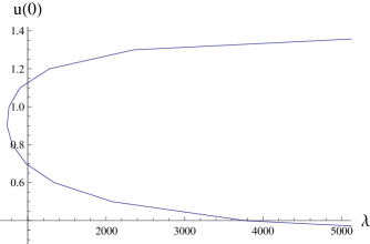
Figure 1: The solution curve for the problem (3.17)

Example $1$ We solved numerically the problem (3.16), with $n=3$, $M=4$, $2M-1=7$

(3.17) $$u^{\prime\prime}+\frac{2}{r}u^{\prime}+\lambda\left(u^{4}+u^{7}\right)=0\,,\;\;\;u^{\prime}(0)=u(1)=0\,.$$

(See [9] for the exposition of the shoot-and-scale algorithm that we used.) The solution curve is presented in Figure $1$. Observe that the $\lambda$’s in this picture are larger than for most other $f(u)$, see [9]. We have verified this numerical result by an independent computation. Taking an arbitrary point $(\bar{\lambda},\bar{u})$ on the solution curve, we solved numerically the initial value problem for the equation in (3.17), with $\lambda=\bar{\lambda}$, using the initial conditions $u(0)=\bar{u}$, $u^{\prime}(0)=0$. The first root of the solution was always at $r=1$.

Example $2$ We solved numerically the problem

(3.18) $$u^{\prime\prime}+\frac{2}{r}u^{\prime}+\lambda\left(u^{3}+u^{7}\right)=0\,,\;\;\;u^{\prime}(0)=u(1)=0\,.$$

Compared with the Example $1$, only the lower power is changed from $4$ to $3$. Not only the solution curve, presented in Figure $2$, has a different shape, $\lambda$’s are now much smaller, while $u(0)$’s go higher. We conjecture that there are still exactly two positive solutions for $\lambda$ large enough.

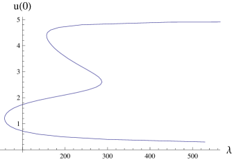
Figure 2: The solution curve for the problem (3.18)

We turn next to the $p$-Laplace version of Bratu’s equation

(3.19) $$\varphi\left(u^{\prime}(r)\right)^{\prime}+\frac{n-1}{r}\varphi\left(u^{\prime}(r)\right)+Be^{u}=0\,,$$

where $\varphi\left(z\right)=z|z|^{n-1}$ (i.e., $p=n$), and $B>0$ is a constant. Set here

$$\varphi\left(u^{\prime}(r)\right)=-are^{\frac{n-1}{n}u}\,,$$

where $a>0$ is a constant. Then $-u^{\prime}=a^{\frac{1}{n-1}}r^{\frac{1}{n-1}}e^{\frac{1}{n}u}$. It follows that

$$\varphi\left(u^{\prime}(r)\right)^{\prime}=-ae^{\frac{n-1}{n}u}-\frac{n-1}{n}are^{\frac{n-1}{n}u}u^{\prime}=-ae^{\frac{n-1}{n}u}+\frac{n}{n-1}a^{\frac{n}{n-1}}r^{\frac{n}{n-1}}e^{u}\,.$$

We use these expressions in (3.19), and solve for $u$:

(3.20) $$u(r)=n\ln\left(\frac{a\,n}{B+\frac{n}{n-1}a^{\frac{n}{n-1}}r^{\frac{n}{n-1}}}\right)\,.$$

One verifies that this function is a solution of (3.19) for any $a>0$, $B>0$, and $n>1$. This family of exact solutions immediately implies the exact count of solutions for the corresponding Dirichlet problem on the unit ball in $R^{n}$.

Proposition 2

For the problem

$$\varphi\left(u^{\prime}(r)\right)^{\prime}+\frac{n-1}{r}\varphi\left(u^{\prime}(r)\right)+Be^{u}=0\,,\;\;u^{\prime}(0)=u(1)=0\,,$$

where $\varphi\left(z\right)=z|z|^{n-1}$ (i.e., $p=n$), there is a constant $B(n)>0$, so that there are exactly two solutions for $0<B<B(n)$, exactly one solution for $B=B(n)$, and no solutions if $B>B(n)$.

Proof:    According to the formula (3.20), the boundary condition $u(1)=0$ is equivalent to $a$ satisfying

$$\frac{n}{n-1}a^{\frac{n}{n-1}}+B=n\,a\,.$$

On the left we have a convex superlinear function of $a$, so that there is a constant $B=B(n)$, such that this equation has two solutions for $0<B<B(n)$, one solution for $B=B(n)$, and none if $B>B(n)$. $\diamondsuit$

4 A change of variables

For the non-autonomous problem (here $\alpha$, and $a>0$ are constants)

(4.1) $$u^{\prime\prime}+\frac{n-1}{r}u^{\prime}+r^{\alpha}f(u)=0\,,\;\;u(0)=a\,,\;\;u^{\prime}(0)=0\,,$$

we present a change of variables which essentially eliminates the non-autonomous term $r^{\alpha}$ (although it changes the spatial dimension).

Proposition 3

Let $u(r)\in C^{2}(0,b)\cap C^{1}[0,b]$ be a solution of (4.1), with some $b>0$, and assume that $\alpha>-1$. The change of variables $t=\frac{r^{1+\alpha/2}}{1+\alpha/2}$ transforms the problem (4.1) into

(4.2) $$u^{\prime\prime}(t)+\frac{m}{t}u^{\prime}(t)+f(u(t))=0\,,\;\;u(0)=a\,,\;\;\frac{du}{dt}(0)=0\,,$$

with $m=\frac{n-1+\alpha/2}{1+\alpha/2}$.

Proof:    We have $u_{r}=u_{t}r^{\alpha/2}$, $u_{rr}=u_{tt}r^{\alpha}+\frac{\alpha}{2}u_{t}r^{\frac{\alpha}{2}-1}$, and (4.1) becomes

$$u_{tt}r^{\alpha}+\frac{\alpha}{2}u_{t}r^{\frac{\alpha}{2}-1}+(n-1)u_{t}r^{\frac{\alpha}{2}-1}+r^{\alpha}f(u)=0\,.$$

Dividing by $r^{\alpha}$, we get the equation in (4.2).

To see that $\frac{du}{dt}(0)=0$, we rewrite (4.1) as $\left(r^{n-1}u^{\prime}\right)^{\prime}+r^{\alpha+n-1}f(u)=0$, and then express

$$u^{\prime}(r)=-\frac{1}{r^{n-1}}\int_{0}^{r}z^{\alpha+n-1}f(u(z))\,dz\,.$$

We have

$$\frac{du}{dt}(0)=\lim_{r\rightarrow 0}\frac{u^{\prime}(r)}{r^{\alpha/2}}=-\lim_{r\rightarrow 0}\frac{1}{r^{n-1+\alpha/2}}\int_{0}^{r}z^{\alpha+n-1}f(u(z))\,dz=0\,.$$

$\diamondsuit$

Observe that in case $n=2$, we have $m=n-1=1$, which means that the $r^{\alpha}$ term is eliminated without changing the dimension. We also remark that for $\alpha\leq-1$, we do not expect the problem (4.1) to have solutions of class $C^{2}(0,b)\cap C^{1}[0,b]$, as an explicit example below shows.

Example The problem

$$u^{\prime\prime}(t)+\frac{1}{t}u^{\prime}(t)+e^{u}=0\,,\;\;u(0)=a\,,\;\;u^{\prime}(0)=0$$

has a solution $u(t)=a-2\ln\left(1+\frac{e^{a}}{8}t^{2}\right)$ going back to the paper of G. Bratu [3] from 1914, see also J. Bebernes and D. Eberly [2]. (Letting here $a=\ln 8\left(3\pm 2\sqrt{2}\right)$, one gets two solutions of the corresponding Dirichlet problem on the unit ball, with $u(1)=0$.) Setting here $t=\frac{r^{1+\alpha/2}}{1+\alpha/2}$, we see that

(4.3) $$u(r)=a-2\ln\left(1+\frac{e^{a}}{8\left(\frac{\alpha}{2}+1\right)^{2}}\,r^{\alpha+2}\right)$$

is the solution of the problem

(4.4) $$u^{\prime\prime}(r)+\frac{1}{r}u^{\prime}(r)+r^{\alpha}e^{u}=0\,,\;\;u(0)=a\,,\;\;u^{\prime}(0)=0\,.$$

This explicit solution is of particular importance for singular equations, when $\alpha<0$, showing us what to expect for more general nonlinearities than $e^{u}$. In the mildly singular case, when $-1<\alpha<0$, the function in (4.3) is still a solution of (4.4), although it is not classical, but only of class $C^{1,1+\alpha}$. In the strongly singular case, when $\alpha<-1$, the function in (4.3) has unbounded derivative as $r\rightarrow 0$. The case of Coulomb potential, when $\alpha=-1$, is very special. The corresponding solution from (4.3)

$$u(r)=a-2\ln\left(1+\frac{e^{a}}{2}r\right)$$

still satisfies $u(0)=a$, but not $u^{\prime}(0)=0$. Instead, we have $u^{\prime}(0)=-e^{a}=-e^{u(0)}$. We see that the initial value problem

(4.5) $$u^{\prime\prime}(r)+\frac{1}{r}u^{\prime}(r)+\frac{1}{r}e^{u}=0\,,\;\;u(0)=a\,,\;\;u^{\prime}(0)=-e^{u(0)}$$

is a natural substitute of the problem (4.4) in case of the Coulomb potential. Problems with the Coulomb potential occur in applications, see J.L. Marzuola et al [12].

We can now extend all of the known multiplicity results for autonomous equations to the non-autonomous equation (4.1). For example, we have the following result for a cubic nonlinearity, which is based on a similar theorem for $\alpha=0$ case, see [10], [13], [9].

Theorem 4.1

Assume that $c>2b>0$, and $\alpha>0$. Then there is a critical $\lambda_{0}$, such that for $\lambda<\lambda_{0}$ the problem

$$u^{\prime\prime}+\frac{n-1}{r}u^{\prime}+\lambda r^{\alpha}u(u-b)(c-u)=0,\;\;r\in(0,1),\;\;u^{\prime}(0)=u(1)=0$$

has no positive solutions, it has exactly one positive solution at $\lambda=\lambda_{0}$, and there are exactly two positive solutions for $\lambda>\lambda_{0}$. Moreover, all solutions lie on a single smooth solution curve, which for $\lambda>\lambda_{0}$ has two branches, denoted by $u^{-}(r,\lambda)<u^{+}(r,\lambda)$, with $u^{+}(r,\lambda)$ strictly monotone increasing in $\lambda$, and $\lim_{\lambda\rightarrow\infty}u^{+}(r,\lambda)=c$ for all $r\in[0,1)$. For the lower branch, $\lim_{\lambda\rightarrow\infty}u^{-}(r,\lambda)=0$ for $r\neq 0$. (All of the solutions are classical.)

A similar transformation works for the $p$-Laplace case

(4.6) $$\;\;\;\;\varphi\left(u^{\prime}(r)\right)^{\prime}+\frac{n-1}{r}\varphi\left(u^{\prime}(r)\right)+r^{\alpha}f(u(r))=0\,,\;\;u(0)=a\,,\;\;u^{\prime}(0)=0\,,$$

where $\varphi(z)=z|z|^{p-2}$, with $p>1$.

Proposition 4

Let $u(r)\in C^{2}(0,b)\cap C^{1}[0,b]$ be a solution of (4.6), with some $b>0$, and assume that $\alpha>-1$. The change of variables $t=\frac{r^{1+\alpha/p}}{1+\alpha/p}$ transforms the problem (4.6) into

(4.7) $$\varphi\left(u^{\prime}(t)\right)^{\prime}+\frac{m}{t}\varphi\left(u^{\prime}(t)\right)+f(u(t))=0\,,\;\;u(0)=a\,,\;\;\frac{du}{dt}(0)=0\,,$$

with $m=\frac{n-1+\alpha-\alpha/p}{1+\alpha/p}$.

Proof:    We have $u_{r}=u_{t}r^{\alpha/p}$, $\varphi\left(u_{r}\right)=r^{\alpha-\alpha/p}\varphi\left(u_{t}\right)$, and

$$\frac{d}{dr}\varphi\left(u_{r}\right)=(\alpha-\alpha/p)r^{\alpha-\alpha/p-1}\varphi\left(u_{t}\right)+r^{\alpha-\alpha/p}\frac{d}{dt}\varphi\left(u_{t}\right)r^{\alpha/p}\,,$$

which leads us to (4.7).

To see that $\frac{du}{dt}(0)=0$, we rewrite (4.6) as $\left(r^{n-1}\varphi\left(u^{\prime}\right)\right)^{\prime}+r^{\alpha+n-1}f(u)=0$, and then express

(4.8) $$-u^{\prime}(r)=\left[\frac{1}{r^{n-1}}\int_{0}^{r}z^{\alpha+n-1}f(u(z))\,dz\right]^{\frac{1}{p-1}}\,.$$

We have

$$-\frac{du}{dt}(0)=\lim_{r\rightarrow 0}\frac{-u^{\prime}(r)}{r^{\alpha/p}}=\lim_{r\rightarrow 0}\left[\frac{\left(-u^{\prime}(r)\right)^{p-1}}{r^{\frac{\alpha}{p}(p-1)}}\right]^{\frac{1}{p-1}}\,,$$

and by (4.8)

$$\lim_{r\rightarrow 0}\frac{\left(-u^{\prime}(r)\right)^{p-1}}{r^{\frac{\alpha}{p}(p-1)}}=-\lim_{r\rightarrow 0}\frac{1}{r^{n-1+\alpha-\alpha/p}}\int_{0}^{r}z^{\alpha+n-1}f(u(z))\,dz=0\,,$$

completing the proof. $\diamondsuit$

In case $n=p$, we have $m=n-1$, which means that the $r^{\alpha}$ term is eliminated without changing the dimension.

References

[1]
T. Aubin, Problèmes isopérimétriques et espaces de Sobolev, (French) J. Differential Geometry11, no. 4, 573-598 (1976).
[2]
J. Bebernes and D. Eberly, Mathematical Problems from Combustion Theory. Applied Mathematical Sciences, 83, Springer-Verlag, New York, 1989.
[3]
G. Bratu, Sur les equations integrales non lineares, Bull. Soc. Math. de France42, pp. 113-142 (1914).
[4]
H. Brézis and L. Nirenberg, Positive solutions of nonlinear elliptic equations involving critical Sobolev exponents, Comm. Pure Appl. Math.36, no. 4, 437-477 (1983).
[5]
N. Ghoussoub and Y. Guo, On the partial differential equations of electrostatic MEMS devices: stationary case, SIAM J. Math. Anal.38, no. 5, 1423-1449 (2007).
[6]
Z. Guo and J. Wei, Infinitely many turning points for an elliptic problem with a singular non-linearity, J. Lond. Math. Soc. (2)78, no. 1, 21-35 (2008).
[7]
P. Korman, Existence and uniqueness of solutions for a class of -Laplace equations on a ball, Adv. Nonlinear Stud.14, no. 9-10, 963-984 (2009).
[8]
P. Korman, Global solution curves for self-similar equations, J. Differential Equations257, no. 7, 2543-2564 (2014).
[9]
P. Korman, Global Solution Curves for Semilinear Elliptic Equations, World Scientific, Hackensack, NJ (2012).
[10]
P. Korman, Y.Li and T. Ouyang,
An exact multiplicity result for a class of
semilinear equations, Commun. in PDE22, 661-684 (1997).
[11]
C.S. Lin and W.-M. Ni, A counterexample to the nodal domain conjecture and related semilinear equation, Proc. Amer. Math. Soc.102, 271-277 (1988).
[12]
J.L. Marzuola, S.G. Raynor and G. Simpson, Existence and stability properties of radial bound states for Schrödinger-Poisson with an external Coulomb potential in three dimensions, ArXiv:1512.03665v2 (2015).
[13]
T. Ouyang and J. Shi,
Exact multiplicity of positive solutions for a class of semilinear problems, II, J. Differential Equations158, no. 1, 94-151 (1999).
[14]
J.A. Pelesko, Mathematical modeling of electrostatic MEMS with tailored dielectric properties, SIAM J. Appl. Math.62, no. 3, 888-908 (2002).
[15]
G. Talenti, Best constant in Sobolev inequality, Ann. Mat. Pura Appl.110 (4), 353-372 (1976).