Computing the Oja Median in R:
The Package OjaNP
Abstract
The Oja median is one of several extensions of the univariate median to the multivariate case. It has many nice properties, but is computationally demanding. In this paper, we first review the properties of the Oja median and compare it to other multivariate medians. Afterwards we discuss four algorithms to compute the Oja median, which are implemented in our R-package OjaNP. Besides these algorithms, the package contains also functions to compute Oja signs, Oja signed ranks, Oja ranks, and the related scatter concepts. To illustrate their use, the corresponding multivariate one- and -sample location tests are implemented.
Keywords
Oja median, Oja signs, Oja signed ranks, Oja ranks, R,C,C++
1 Introduction
The univariate median is a popular location estimator. It is, however, not straightforward to generalize it to the multivariate case since no generalization known retains all properties of univariate estimator, and therefore different generalizations emphasize different properties of the univariate median. So besides the Oja median described here, there are several other multivariate median concepts. Hayford [1902] suggested the first generalization by simply using the vector of the marginal medians. Other popular multivariate medians are Tukey’s median [Tukey, 1975] and the spatial median (also known as median). The spatial median was initially defined as a bivariate median [Weber, 1909, 1929] and subsequently extended to the general multivariate case. These and more multidimensional medians are surveyed in Small [1990] and Oja [2013]. While the vector of marginal medians is quite easy to compute, the other multivariate medians are a more computationally expensive. Particularly the Oja median [Oja, 1983] has, despite its compelling statistical properties, not been used very often in practice so far, since it is difficult to compute. The main topic of this paper is to describe the OjaNP [Fischer et al., 2016] package, which provides several algorithms for the computation of the Oja median in R [R Core Team, 2016].
The outline of this paper is as follows. In Section 2.1, we review and compare some multivariate medians and show which properties of the univariate median is generalized by which multivariate median. Our main focus is on the Oja median, whose basic properties are discussed in Section 2.2, followed by an introduction to Oja signs and ranks (Section 2.3), Oja signed ranks (Section 2.4) and Oja sign and rank covariance matrices (Section 2.5). To demonstrate the application of the Oja median and its sign and rank concepts, Section 2.6 discusses one- and -sample tests of location.
In Section 3, we focus on the different algorithms provided by the package OjaNP to calculate the Oja median. Four different algorithms are available: two exact algorithms and two approximate algorithms based on different designs.
Chapter 4 shows how to use the package OjaNP in order to calculate the Oja median and related statistics. We provide simple examples, and additional benchmarks are calculated to analyze the performance of the implementations.
A concept frequently encountered in this paper is affine equivariance. We use it in the sense of full-rank affine equivariance, which is common in robust statistics. Given the -dimensional sample we let be the data matrix of dimension , containing the data points as rows. Subsequently the data sample is identified with . For a given affine-linear transformation , with and non-singular, the data matrix of the transformed data is given by
where denotes the vector consisting of ones. We call an -valued location statistic affine equivariant, if
| (1) |
This applies analogously to set-valued location statistics , such as median sets. For a matrix-valued scatter statistic taking on values in , affine equivariance is commonly understood as
2 Oja median and related concepts
2.1 Oja median and other multivariate medians
We start by introducing the univariate median for distributions. Given a distribution function , let
Then the median (set) of is given by the interval
| (2) |
Any point of the interval divides the distribution in two halves of equal probability weight and can represent the median. In case a unique selection is needed, we use the gravity center of the median set as a (single-point) median and denote it by the lower case symbol,
| (3) |
For a given sample , the median is obtained as
with being the -th order statistic. The latter definition is a special case of (3), obtained by taking to be the empirical distribution of , which gives equal probability mass to each of the points . Note that is an affine equivariant location statistic.
Now let be a -dimensional dataset, where denotes the -th column of and corresponds hence to the -th variable. The many existing notions of a -variate median for such data have in common that they reduce to the univariate median for . Multivariate medians are generally non-unique, and we select, as above, the gravity center of the median set to obtain a unique representation.
To the best of our knowledge the first generalization of the univariate median to the multivariate case is the vector of marginal medians described in Hayford [1902].
Definition 1.
The vector of marginal medians of the sample is defined as
The vector of marginal medians is easily computed but not affine equivariant. A simple rotation of two-dimensional data visualizes the problem. In the left part of Figure 1 a two-dimensional dataset is plotted and rotated around the point +. At the same time the marginal median is continuously plotted. An affine equivariant median would follow the rotation on a circle. The blue circle represents the Oja median and illustrates the behavior of an affine equivariant median. In the right part of Figure 1 we visualize the behavior of a rotation invariant estimator that is not scale invariant. We use the spatial median for this example, see Definition 3 below.

The second generalization of the univariate median reviewed here is based on the fact that for a given sample and its median the equation
holds, where if and otherwise. This means, there are as many observations smaller than as are bigger, as it was pointed out e.g. in Hotelling [1929]. Given a -dimensional dataset, we consider halfspaces in every direction . Let denote the “minimal” halfspace with normal vector that contains at least half of the data points, i.e., for any other halfspace with these properties holds. The intersection of all , forms the Tukey median Tmed(). If the data are in general position, each such halfspace is bordered by a hyperplane through exactly data points, and the Tukey median is in general no singleton. (A set of -variate data is in general position if at most of them lie on the same hyperplane.) The unique Tukey median tmed() is defined as the gravity point of this median set; see Tukey [1975] and Donoho and Gasko [1992]. It is affine equivariant [Chen, 1995] and can be introduced as the maximizer of a depth function as follows.
Definition 2.
Let be a -dimensional sample as above. For any ,
| (4) |
is called the Tukey depth or location depth of w.r.t. . (Here denotes the cardinality of a set .) The Tukey median Tmed of the sample is defined as the maximizer of the Tukey depth,
| (5) |
Another way to generalize the univariate median is to transfer its minimizing feature into higher dimensions. Consider again a univariate sample in . When minimizing the sum over we obtain
| (6) |
This minimizing feature of the univariate median is interpretable in two ways: it is the sum of absolute deviations, but it can also be viewed as the sum of one-dimensional simplices. The first interpretation will lead us to the spatial median, the second to the Oja median.
The spatial median is presumably the most popular multivariate median and almost as old as the marginal median. Weber [1909] first described the spatial median and used it to solve an economic problem: he was looking for the best place of a distribution center in the sense, that the sum of distances between outposts and the distribution center becomes minimal. The -dimensional extension of this approach is the spatial median.
Definition 3.
The spatial median of a -variate data sample is defined as
| (7) |
Here denotes the Euclidean norm. The spatial median is sometimes also referred to as the median since it minimizes the norm of the -variate vector of distances . The spatial median is not affine equivariant as is visualized in the right part of Figure 1. Given an affine transformation which transforms the data points from the left star-shaped figure into the right star-shaped figure, the center of each star is the spatial median of the data points. However, due to the lack of affine equivariance, the transformed spatial median (marked with the arrow) does not coincide with the spatial median of the transformed data set. The spatial median is rotation invariant, but not scale invariant.
Oja [1983] introduced a multivariate median based on volumes of simplices. A -dimensional simplex is the convex hull of spanning points in general location. Let
be points in general location from . The volume of the simplex spanned by the points is then given by
| (8) |
see, e.g., Stein [1966]. Let be a distribution on having finite first moment. The Oja median of is defined as follows: for i.i.d. random vectors , each distributed with , define the Oja median set as
For data we have the following definition. Let
| (9) |
be the set of all ordered -tuples out of , .
Definition 4.
The Oja median Omed of a -dimensional sample of size is defined as
| (10) |
This means that the Oja median of a -dimensional sample is any point for which the sum of simplex volumes over all combinations of possible data points is minimal. Note that equals , where is the empirical distribution on . A unique version of the Oja median, denoted , is obtained by selecting the point of gravity of .
2.2 Properties of the Oja median
As other multivariate extensions of the median, the Oja median is not unique. In the bivariate case, we have the following result.
Theorem 1.
If is even and the data points are in general position, then the Oja median is unique.
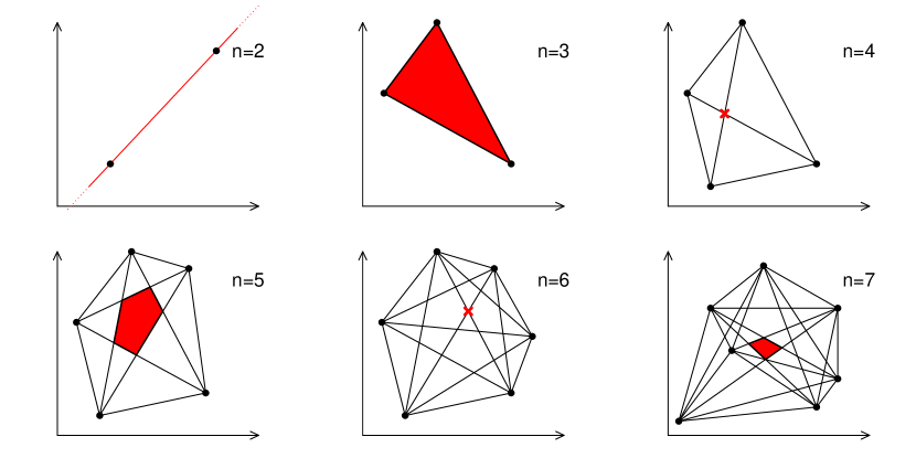
For details see Niinimaa [1995]. The author also identifies a necessary and sufficient condition for the bivariate Oja median to be unique if is odd. There appears to be no result for higher dimensions, but Oja [1999] conjectures that the Oja median is unique for even (odd) sample sizes if the dimension is even (odd). Figure 2 visualizes the Oja Median in several small-sample data situations.
Theorem 2.
The Oja median of a sample is a convex set.
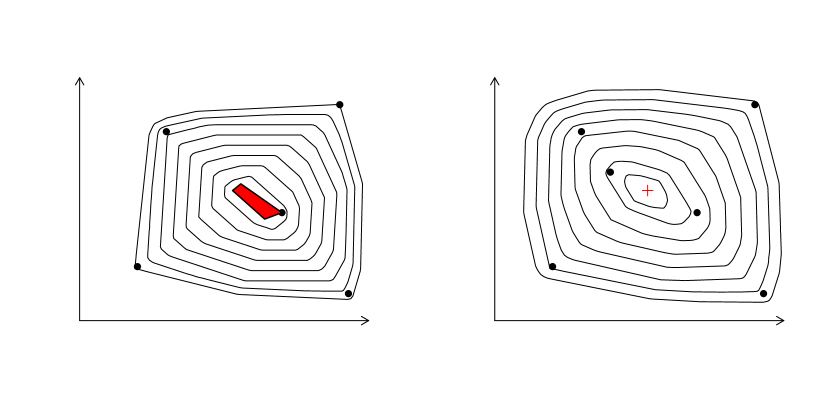
See Oja and Niinimaa [1985] for details. Theorem 2 is illustrated in Figure 3. Contour lines of the objective function (10) are plotted for two small data clouds. The objective function is convex for, both, even and odd sample sizes.
Theorem 3.
The Oja median is affine equivariant.
Hence the Oja median is proper location statistic in the sense of (1), i.e., . The next result can be found, e.g., in Arcones et al. [1994], Shen [2008].
Theorem 4.
Under mild regularity conditions (including the existence of first moments) for an i.i.d. sample from the distribution , we have
where is the Oja sign covariance matrix (OSCM) defined later in Section 2.5 at and is the expected covariance matrix between the Oja signs (, see Section 2.3) and the optimal location score of .
Concerning robustness the Oja Median has the following properties.
Theorem 5.
Let have a finite first moment. Then the Oja median has a bounded influence function.
The influence function is for example given in Niinimaa and Oja [1995]. The Oja median has an asymptotic breakdown point of 0. Niinimaa et al. [1990] show the following:
Theorem 6.
The finite-sample breakdown-point of the bivariate Oja median is .
Table 1 summarizes the main properties of the Oja median and other common multivariate medians discussed here. For another recent discussion of the different medians see also Oja [2013].
| Median | Affine Equivariance | Breakdown Point |
| Marginal Median | No | |
| Tukey Median | Yes | |
| Spatial Median | No | |
| Oja Median | Yes | 0 |
| Influence function | Asymptotic distribution | |
| Marginal Medians | Niinimaa and Oja [1995] | Babu and Rao [1988] |
| Tukey Median | Romanazzi [2001] | Bai and He [1999] |
| Spatial Median | Niinimaa and Oja [1995] | Möttönen et al. [2010] |
| Oja Median | Niinimaa and Oja [1995] | Shen [2008] |
2.3 Oja signs and ranks
Closely related to the median is the concept of signs and ranks. In this subsection we introduce the multivariate Oja sign and Oja rank and relate them to other multivariate signs and ranks, corresponding to the marginal and the spatial median. Again, to motivate the subsequent derivations we take a brief look at the univariate case. Suppose we have a univariate data set , . We call
| (11) |
the sign of w.r.t. the data sample , where is the univariate sign function ( if and zero otherwise), and is the univariate median of the sample . There are several possibilities of suitably assigning ranks to the data points. By
| (12) |
we define normalized central ranks, which may take on possible values ranging from -1 to 1. In the following we call simply the rank of w.r.t. .
The median appropriately centers the data. I.e., the signs of the data points, centered by the median, sum up to zero:
| (13) |
(Note that the mean does the same for the data points themselves.) In other words we may say that the median has central rank zero,
| (14) |
and, in this respect, is the most central point. Identities (13) and (14) (which are different formulations of the fact that half of the data lies above and below the median) provide the essential link between signs and ranks and the median and are a motivating principle behind the multivariate sign and rank functions we will introduce next. Note that a -variate sign function should be a vector that can point in any direction of the -dimensional space. The same holds for a multivariate rank function based on signs.
An obvious extension of (11) to the multivariate setting is its componentwise application, leading to the marginal sign function. We call
the marginal sign of w.r.t. the -variate data sample , where ,
and is the marginal median of . An equally straightforward generalization is the spatial sign of w.r.t. :
where
and is the spatial median of . The corresponding rank functions, the marginal rank and the spatial rank , are obtained by replacing in (12) by and , respectively. The Oja sign is defined as follows. For , let and as in . We call
the Oja sign of the point w.r.t. the data sample and the center location and
| (16) |
simply the Oja sign of w.r.t. . Furthermore
| (17) | |||||
is the Oja rank of w.r.t. . The notation means the gradient (the derivative as a column vector) w.r.t. . We define the derivative of to be zero at the origin, i.e., , .
We note a qualitative difference in the definition of the Oja sign to the marginal and the spatial sign. The Oja sign function depends on the sample not only through the centering point , but is a function of the whole sample. By introducing the parameter in definition (2.3) we allow the data to be centered by a different central location than the Oja median. This may be useful under some circumstances, for example to speed up computation. The function ojaSign offers this option.
We also note that for expressions (16) and (17) reduce to
and
hence and are proper generalizations of and , respectively, in the sense that for they coincide with their univariate counterparts.
In dimensions 2 and 3 Oja signs and ranks allow a descriptive geometric interpretation. The key is to recall that the -dimensional volume of the simplex spanned by points in is given by , cf. (8), and that hence
characterizes all points that lie on the dimensional hyperplane spanned by the points . Then, for (), is the average of the -dimensional vectors , , where
-
•
is perpendicular to the plane (straight line) going through the points and ,
-
•
has length equal to times the area (length) of the triangle (line segment) that is bordered by the points and
-
•
points from the plane (straight line) to the point .
If itself lies on the plane (straight line) or if the points do not uniquely determine a plane (straight line), the vector is zero. Likewise, is the average of vectors , each perpendicular to the the plane (straight line) spanned by .
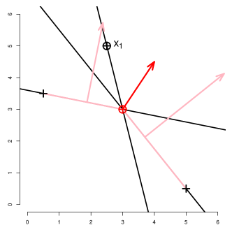
The construction of the Oja sign is visualized in Figure 4 at the very simple example of three points in : The red is an interior point (let it be denoted by ) of the Oja median set, which is simply the triangle bordered by the three data points. Then , the vector in red, is formed as the average of the two light red vectors and the null vector (the latter being interpreted as a vector pointing perpendicularly from the straight line — to ). In this example, is invariant w.r.t. the specific choice of as long as is below both lines — and —.
As in the univariate case, cf. (13) and (14), the multivariate signs of the data points sum up to zero, i.e.,
where may be any of , or . Equivalently,
| (18) |
where may be any of , or , and the respective multivariate median. This is generally only true if the appropriate median is chosen as centering point, for Oja signs in particular, the data has to be centered by the Oja median. Some further care must be given to these statements. If the median set is no singleton, they may be false for median points on its border. This also happens in the univariate case, when, for an even number of observations, one chooses the median to be or . The function ojaMedian is likely to return points at the border of the median set. In (7) and (10), respectively, the spatial median and the Oja median were introduced as minimizers of objective functions, both generalizing the univariate case (6). Spatial and Oja ranks may be introduced as derivatives of these objective functions. Thus (18) is in concordance with the optimality property of the medians.
The negative rank function defines a hyperplane through , on the positive side of which the Oja median is found. This property is used by the exact bounded algorithm (Section 3.2) to reduce the search region for the median.
Similar to the multivariate medians, the multivariate signs differ by their equivariance and invariance properties. All multivariate signs are translation invariant, i.e., for , , we have
where, again, is any of , , . Marginal signs are furthermore invariant w.r.t. monotonously increasing, componentwise transformations, in particular
for with , . Spatial signs on the other hand are equivariant under orthogonal transformations, i.e.,
for any orthogonal . Oja signs even obey a form of affine equivariance, an inverse proportional affine equivariance:
| (19) |
for any non-singular , and they appear in the literature under the name affine equivariant signs. The respective multivariate rank functions have analogous equivariance and invariance properties. More details on Oja signs and ranks and their applications can be found, e.g., in Oja [1999]. Hettmansperger and McKean [2011] give an overview of multivariate sign and rank methods in general, Puri and Sen [1971] treat methods based on marginal signs and ranks and Oja [2010] describes spatial sign and rank methods.
2.4 Oja signed ranks
As in the Section 2.3 we consider first the univariate case. Suppose we have a univariate data set . The signed rank of w.r.t. can be defined by
| (20) |
where . Note that the signed rank of the -th observation can be written as
| (21) |
where is ranked among absolute values . The Wilcoxon signed rank statistic is thus asymptotically equivalent with .
The signed rank can be extended to the multivariate case, provided we have a concept of multivariate sign. We get spatial signed rank if we replace in (20) by . The Oja signed rank can be defined in the following way. Let be the set of possible vectors , i.e., . Then
| (22) |
is the Oja signed rank of w.r.t. . It is easy to see that the Oja signed rank coincides with the univariate signed rank when . Furthermore, it can be shown that
-
•
is odd: .
-
•
points (approximately) in the direction of .
-
•
.
-
•
is bounded, piecewise constant and increases in magnitude as moves away from .
2.5 Oja sign and rank matrices
Multivariate signs can be useful for obtaining information about the spread of the data and dependencies among the variables. We call
the Oja sign covariance matrix of w.r.t. the central location ,
the Oja sign covariance matrix of and
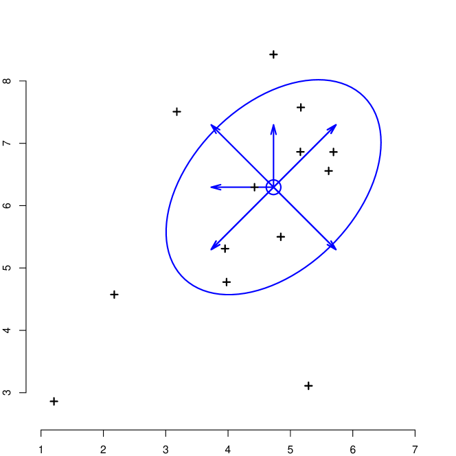
the Oja rank covariance matrix of . In an analogous way we define marginal and spatial sign and rank matrices and by replacing by , and by and , respectively. A comparative study of all sign and rank matrices presented here can be found in Visuri et al. [2000]. Figure 5 shows a small two-dimensional data sample, together with the different multivariate medians and the corresponding signs and sign covariance matrices visualized as ellipses. The ellipses have radius , i.e. the positive definite matrix is depicted by the ellipse .
a)

b)
c) 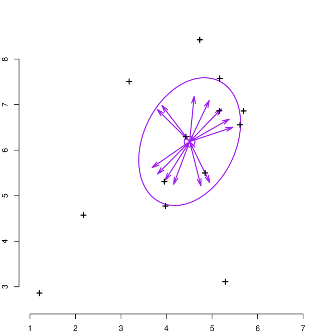
d) 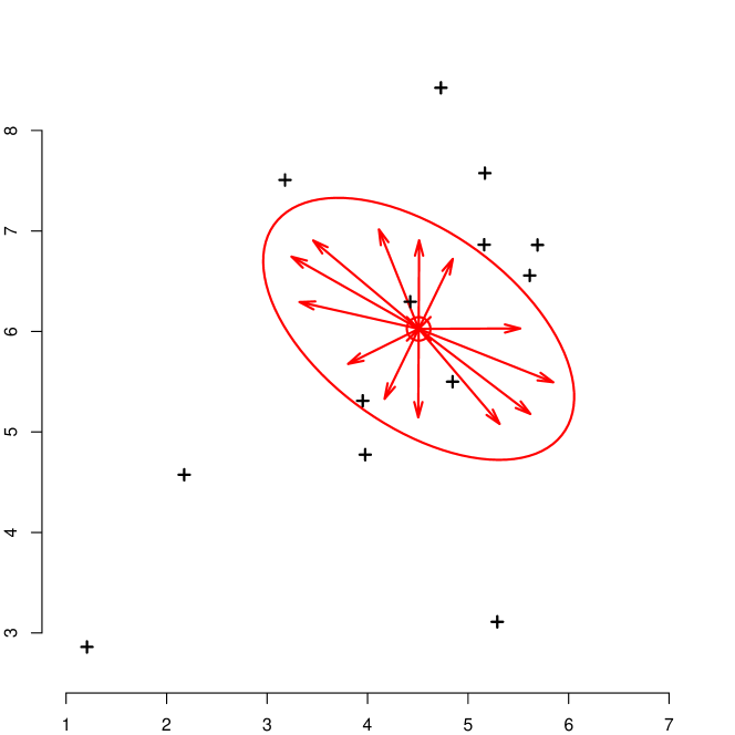
The affine equivariance (19) for Oja signs and ranks translates into a similar equivariance for the corresponding covariance matrices,
and
for and with full rank. This has, roughly speaking, the consequence that OSCM and ORCM estimate the inverse of the covariance matrix up to scale. More specifically, Ollila et al. [2003] show that converges to a multiple of the inverse of the covariance matrix at the rate, if is a -convergent location estimator and the data stem from a linear transformation of a reflection and permutation invariant distribution having finite second moments. The statistical theory of the Oja rank covariance matrix ORCM is treated in Visuri et al. [2003] and Ollila et al. [2004].
A further consequence of this remarkable property is that Oja sign and rank matrices provide easily-obtained, positive definite, consistent estimates for the covariance matrix up to scale, which is a significant advantage over the other sign and rank covariance matrices. Multivariate data analysis is primarily aimed at analyzing the dependencies and interactions between variables. For multivariate methods such as correlation, canonical correlation analysis, principal component analysis, or factor analysis, it is fully sufficient to know the covariance matrix only up to scale. In particular, the OSCM and the ORCM directly estimate a multiple of the concentration matrix or precision matrix, i.e., the inverse covariance matrix, which plays an important role in graphical models. The application of OSCM in this context is examined in Vogel et al. [2008] and Vogel and Fried [2008]. Due to their (inverse proportional) affine equivariance, the theory developed in Vogel and Fried [2011] also applies to the OSCM and the ORCM.
Furthermore Ollila et al. [2003] and Ollila et al. [2004] also derive the limiting distributions of OSCM and ORCM in the elliptical model. Contrary to the other non-parametric covariance matrices based on marginal and spatials signs and ranks, the OSCM and the ORCM are not invariant w.r.t. the elliptical generator within the elliptical model. Their asymptotic distribution depends on the tail behavior of the population distribution. But, and this is also in contrast to marginal and spatial non-parametrics, Oja sign and rank matrices are very efficient at the normal model in low dimensions. Their performance almost equals that of the empirical covariance matrix, the normal maximum likelihood estimator. They outperform the empirical covariance matrix ECM at heavier tailed distributions, but are generally less efficient at light tails. They maintain the good efficiency at small sample sizes and small dimensions , which is not true for many robust scatter estimators.
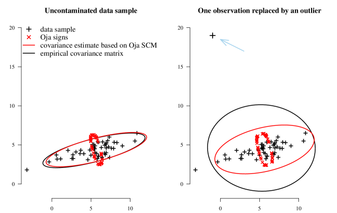
The gain in using the OSCM or the ORCM instead of the sample covariance matrix lies in their higher robustness, which comes at practically no loss in efficiency (but unfortunately at a large increase in computing time). Similar to the Oja median, the Oja sign and rank matrices do not qualify as globally robust estimators in the sense of having a breakdown point near 1/2. They require first moments; their influence functions are unbounded but linear instead of quadratic (as the influence function of the sample covariance matrix), and the asymptotic breakdown point is zero. Very few misplaced observations suffice to let the bias of the estimators become arbitrarily large, but the bias is significantly smaller than that of the sample covariance matrix, cf. Figure 6.
2.6 The one- and -sample location tests based on Oja signs and ranks
The notions of multivariate location and spread together with the corresponding concepts of sign and rank allow the general derivation of multivariate inference methods. The general idea is there to view the signs, signed ranks and ranks as scores, which replace the observations in the classical multivariate procedures. In principle, robust counterparts of any multivariate method can be derived this way. We demonstrate here the multivariate one-sample and -sample location tests. For that purpose, denote for a sample point the corresponding score , where is an optional location w.r.t. to which the score is computed.
2.6.1 The one-sample tests
Assume is a sample of size from a -variate symmetric distribution with symmetry center . We are interested in testing the null hypothesis against .
Denote as the average of the score values under the null hypothesis and . The test statistic is then
Using Oja signs or Oja signed ranks as scores, this yields a straightforward extension of Hotelling’s classical one-sample -test. The test is invariant under affine transformations and asymptotically distribution-free and has a limiting distribution. Test decisions can also be based on permutation principles by randomly changing the signs of the scores. The tests are described in detail in Hettmansperger et al. [1994] and Hettmansperger et al. [1997]. Similar tests can also be naturally constructed using marginal or spatial signs and signed ranks. See Puri and Sen [1971] and Oja [2010] for details.
2.6.2 The -sample tests
Let , , correspond to -variate samples coming from groups having distributions that differ only in location parameters , . The null hypothesis is , i.e., the groups have the same location.
Denote as the combined sample and . Then , , is the average score value of group computed w.r.t. to the location of the combined sample. Similarly, is computed for the combined groups.
The test statistic is obtained as
When Oja signs and Oja ranks are used as scores, -sample tests for multivariate location are obtained that are asymptotically distribution-free and affine invariant. The limiting distribution of the test statistic is , but -values can be obtained by permuting observations between the groups. The two tests are described in Hettmansperger and Oja [1994], Hettmansperger et al. [1998]. Similar tests based on other concepts of signs and ranks are described also in Puri and Sen [1971] and Oja [2010].
3 Description of the algorithms
The package OjaNP contains four different algorithms to calculate the Oja median. Two exact algorithms and two approximate algorithms. The first exact algorithm was developed in Ronkainen et al. [2003] as well as one of the approximate algorithms. The second exact algorithm [Mosler and Pokotylo, 2015] is based on the first one: it accelerates the computation considerably by introducing bounds to the region of search. The numerical calculation is a non-trivial problem which consumes enormous calculation resources and hence, the exact algorithms are limited to small data situations only and, as a consequence, approximate algorithms are needed. These offer parameters to regulate the speed vs. accuracy trade-off, and the user has to decide from case to case which algorithm to choose with which tuning parameters. In Section 4 we will give an overview over the several options and their effect onto the calculation precision and time. Before that, we are going to describe the four algorithms.
3.1 Exact algorithm
Ronkainen et al. [2003] implemented the ideas from Niinimaa et al. [1992] and generalized them into higher dimensions with the help of the result described in Hettmansperger et al. [1999], whereby the vertices of the Oja median set are always located on intersections of hyperplanes that are spanned by data points.
Ronkainen et al. [2003] constructed a Las Vegas algorithm as follows. (This is a simplified version; a more detailed description can be found in the original paper.)
-
1.
Letbe the set of all-dimensional hyperplanes spanned by thepoints in. -
2.
Take the data pointclosest to the mean as an initialcandidate point. -
3.
Samplehyperplanes out ofsuch that the candidate pointis on their intersection. -
4.
Calculate the Oja depth of each intersection point betweenandthe hyperplanes in. -
5.
Take the pointwith the highest Oja depth as next candidate point forthe Oja median. -
6.
Repeat steps 3 to 5 until no improvement in the objective function ispossible (or latest afterrepetitions). -
7.
The result for the exact Oja median is the last candidate point.
Ronkainen et al. [2003] focused on computational stability rather than efficiency. In case a candidate point is a data point, there are possible intersection hyperplanes . Instead of only following the one determined by the gradient of the objective function, the algorithm tries all possible ones.
This algorithm finds just one of the vertices of the median set. While searching for the median, the algorithm may pass through several vertices of the median set, although it is not guaranteed that it visits all of them. The reason is that on step 5 only the first of possibly two points having highest Oja depth is taken as . However, in case of a non-unique median, there exist two such points lying on an edge of the median set. To deliver all vertices of the median set, the algorithm can be modified as follows: it has to store both points as vertices and, in addition, check all lines passing through them.
3.2 Exact bounded algorithm
Based on the exact algorithm of Ronkainen et al. [2003], Mosler and Pokotylo [2015] developed a faster exact algorithm. This algorithm uses the centered rank functions to build bounded regions which contain the median. The negative rank function is a vector that points in a direction of ascent of the depth function. It defines a hyperplane through , on the positive side of which the Oja median is found. The halfspaces defined by the negative rank function are used to build a bounded region that contains the median. In this algorithm, these halfspaces are selected in an iterative way and the further search is restricted to their intersection. The hyperplanes bordering such a search region will be called bounding hyperplanes or simply bounds.
The steps of the algorithm are as follows. (A more detailed description can be found in the original paper):
-
1.
Let be the set of all hyperplanes spanned by the points in .
-
2.
Create the initial rectangular bounded region , limited by hyperplanes that are perpendicular to the coordinate axes and go through the maximal and minimal coordinates of the data points on these axes.
-
3.
Iteratively reduce the bounded region by adding hyperplanes that go through a properly chosen central point of the region and have their normal vectors equal to the corresponding negative rank function. Specifically, the mean value of the bounds’ intersection points is selected as a central point in our implementation. The bounds of that are cut off by newly added hyperplanes are removed.
-
4.
The region is reduced until the desired final volume of the bounded region is reached.
-
5.
Add the bounds from to .
-
6.
-
•
At the first iteration: Take a random initial line on the border of .
-
•
At further iterations: Sample hyperplanes out of in that way, that the candidate point is on their intersection line .
-
•
-
7.
Calculate the Oja depth on each intersection point between and hyperplanes in that lies in the bounded region.
-
8.
Take the point with the highest Oja depth as next candidate point for the Oja median.
-
9.
Repeat steps 6 to 8 until no improvement in the objective function is possible (or latest after repetitions).
-
10.
The result for the exact Oja median is the last candidate point .
The bounded regions reduce the complexity of the searching procedure by reducing the number of hyperplanes that cross the searching lines as well as the number of their intersections to be considered in the minimization procedure.
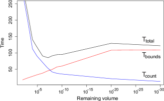
The algorithm is driven by the desired final volume of the bounded region, which is the volume of the minimal rectangle containing the region and having edges parallel to the coordinate axes. As this parameter is reduced, the time needed to build the bounded regions () increases, while the minimization time () decreases along with the number of hyperplanes and their intersections; see Fig. 7. The total computing time () decreases rapidly with the volume, but then slowly grows again. Beyond some point the procedure becomes less efficient. For comparison, the original algorithm needs a total time of ca. 340 seconds in this example. It appears that the fastest computation is obtained if bounds are imposed until the volume of the bounded region ranges around of the original volume. Note that the bounds may cut off some of the vertices of the median set. Moreover, if the central point of the bounded region lies in the median set on step 3, its negative rank function is zero, and this point is directly returned as a median, as on Fig. 9.
Due to limitations in computing memory and long calculation time, the exact algorithm and its bounded version are only able to calculate the Oja median for small datasets in low dimensions. For example, the calculation of the median in a data set of size needs 12 GB RAM. Therefore, approximate algorithms are needed.
Obviously, the bounded algorithm can be stopped at any iteration and some mean value of the last bounded region be taken as an approximation of the Oja median. However, unlike the approximate algorithms presented below, this approach requires the calculation of all hyperplanes. Due to its high computational requirements it is less suited as an approximate algorithm for big data sets in high dimensions.
3.3 Grid-based algorithm
The third algorithm, which calculates an approximation to the Oja median, was also proposed in Ronkainen et al. [2003]. Technically it is a Monte Carlo algorithm. The algorithm lays a uniform grid over the dataset. At each grid point a test is performed whether the point is a possible candidate. The amount of candidate points is reduced as long as only one grid point is left. This point is afterwards the center for a smaller but denser grid, where again each grid point is tested. The algorithm stops when the distance between two grid points gets smaller than a predefined parameter. A second tuning parameter is the significance level of the point tests. The steps of the algorithm are:
-
1.
Create a gridwith equidistant knot distance, covering the wholedataset. -
2.
Choose randomly a set of hyperplanes, build the test statistic and testeach of the grid knots inwhether it is an Oja median. -
3.
Remove those grid knots which have been tested not to be an Oja median. -
4.
If there is more than one knot left, sample additional hyperplanes andrepeat the test for the remaining knots. -
5.
Repeat these steps until only one grid knot is left over. If the lasttest removes all remaining ones, take the last set. -
6.
Build a new grid around the last remaining old grid knot withequidistant knot distance. -
7.
Repeat all these steps until the grid distance reaches a predefinedthreshold. -
8.
The last point is taken as the Oja median.
For further details, especially about the testing procedure, we refer to the original paper Ronkainen et al. [2003]. It may happen that there is continually more than one point left on step 5. In this case sampling of the additional hyperplanes may not help and the algorithm hangs. We restrict the algorithm to 5000 iterations on step 5, after which the grid point with the best test statistic is passed to step 6 and the number of iterations is reduced to 100. We repeat until the grid threshold is reached and return the grid point with the best test statistic as an Oja median approximation.
3.4 Evolutionary algorithm
The fourth algorithm to calculate the Oja median is an evolutionary algorithm, which is based on mutations of the latest candidate points. It was developed by the Department of Computer Science, Efficient Algorithms and Complexity Theory at the TU Dortmund, but has not been published before. The algorithm works as follows:
-
1.
Set the level of initial mutation variance. -
2.
Take 10 randomly chosen observations from. -
3.
Evaluate the objective function for all these points and take the minimumas starting candidate point. -
4.
Chooserandom numbersfrom adistribution andcalculate the-variate mutation vectorThe mutation vectorhas a normally distributed length with given variance
and uniformly distributed direction. -
5.
Calculatemutation pointsforfrom the lastcandidate point. -
6.
Calculate the ratiohow often the objective function is biggerat the mutations than at. -
7.
Ifthenelsefor some. -
8.
Choose as a new candidate point the mutation with the smallest objectivefunction value. -
9.
Repeat steps 4 to 8 until the variance for the next mutation dropsunder a predefined value. -
10.
If the algorithm has not terminated aftersteps, stop the calculation.
Step 7 controls the dynamic of the mutation. If at more than 20% of the mutations the objective function has a smaller value than at the last candidate point, the algorithm increases the variability of the mutation; hence the search area is enlarged. Step 10 ensures that the algorithm terminates in any case.
3.5 Other algorithms for the Oja median in R
There are other implementations of algorithms for the Oja Median available in R, but they are mostly restricted to two dimensions.
The function med in the package depth [Genest et al., 2012] uses the Fortran code of Niinimaa et al. [1992] and is restricted to the bivariate case.
Another method to compute the Oja Median was suggested by Roger Koenker on R-help on 16. Aug 2003 (see http://tolstoy.newcastle.edu.au/R/help/03b/1990.html using the quantreg package [Koenker et al., 2016]:
oja.median <-function(x)
{
##
## bivariate version -- x is assumed to be an n by 2 matrix
##
require(quantreg)
n <- dim(x)[1]
A <- matrix(rep(1:n, n), n)
i <- A[col(A) < row(A)]
j <- A[n + 1. - col(A) > row(A)]
xx <- cbind(x[i, ], x[j, ])
y <- xx[, 1] * xx[, 4] - xx[, 2] * xx[, 3]
z1 <- (xx[, 4] - xx[, 2])
z2 <- - (xx[, 3] - xx[, 1])
return(rq(y~cbind(z1, z2)-1)$coef)
}
4 The R package OjaNP
The main purpose of the OjaNP package is to provide users with the possibility to compute the Oja median. The package includes, however, also other useful functions. The main functions of the package are visualized in Figure 8.
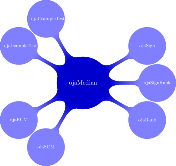
Most of the function names are self-explanatory. For details about them we refer to the corresponding help pages. In the following we will first explain the function ojaMedian and its options in detail. Then we demonstrate the use of some of the functions with a small but illustrative data set, which is also contained in the package.
4.1 The computation of the Oja median in OjaNP
The main function of OjaNP is
ojaMedian(X, alg = "evolutionary", sp = 1, na.action = na.fail,
control = ojaMedianControl(...), ...)
The user can choose via the alg option between four algorithms to calculate the Oja median. Furthermore, we have an option to calculate the Oja median repeatedly and average these results in order to receive less varying results. The amount of repetitions can be controlled with the sp parameter.
In what follows we are going to explain the different parameters which control the flow of the different algorithms in detail and give insights how to choose the parameters in a given data situation. The default algorithm of the ojaMedian function is the evolutionary algorithm.
The evolutionary algorithm loses the affine equivariance property of the Oja median. In order to restore it we first perform a scatter matrix transformation to obtain an invariant coordinate system (implemented in ICS Nordhausen et al. [2008]), apply the algorithm to the transformed data and re-transform afterwards. That way we restore the affine equivariance for this implementation.
Figure 9 shows the exemplary outcome of the four implemented algorithms in simple data situations for the unique (left) and non-unique (right) case. We have chosen simple data situations with 6 and 7 data points, run the different algorithms 500 times and plotted the outcome into the figure.
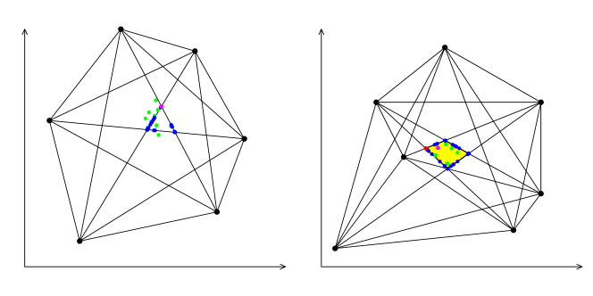
In the left part of Figure 9 we have a data set that has a unique Oja median. This one is correctly determined by the exact implementations (red), whereas both approximate algorithms have a systematic behavior which does not differ strongly from the non-unique case in the right side of the graphic. The evolutionary algorithm (blue) determines the Oja median always along lines of intersection with the result of a bordered area. The right-hand side of Figure 9 exhibits data that have a non-unique Oja median. Here the two exact algorithms find a vertex (red) of the median set, while the evolutionary algorithm (blue) yields any point of the border of the median set, that is the area with the lowest Oja depth (yellow). The grid algorithm, however terminates in this case usually within the convex median set.
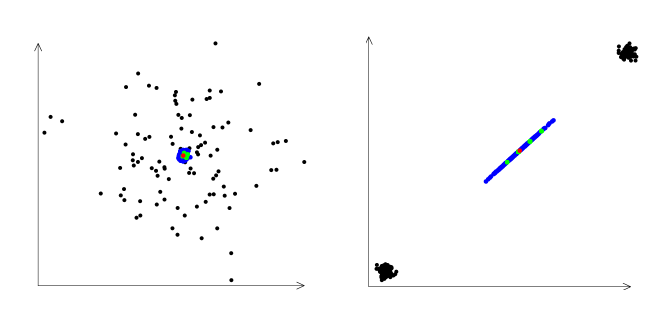
In a next step we are going to analyze the outcome of the algorithms in more complex data situations. The first typical data situation is a multivariate normal distributed data cloud and we calculate the Oja median with the exact (red), the grid (green) and the evolutionary algorithm (blue). As we can see the evolutionary algorithm has the biggest variation within the results, but we have to keep in mind that the default setting of our function is tuned to calculate fast results. In the next paragraph we will discuss how to get more precise results in trade-off for calculation time. For most applications the faster, less accurate settings appear to be preferable.
The second data set of interest consists of two data clouds, which are far away from each other. The motivation for that is to see whether the algorithms take this into account or if they get stuck in one cloud. As you can see in the right part of the figure, that all included algorithms are capable of calculating the Oja median to be in the center between both data clouds.
Let us now compare the runtime of the two approximate algorithms depending on the dimension and size of the data in the bivariate case. We do not perform a runtime analysis for the exact algorithms. Their performance depends strongly on the computer used (particularly memory), much more so than the approximate ones.
On an average computer, bivariate problems up to 1000 observations are solvable in acceptable time, but for higher dimensions and sizes this decision has to be made from case to case. For example in the seven-dimensional case with tens of observations it takes minutes for the exact algorithm to find the solution. The biggest limitation of the exact algorithm is the memory to store all hyperplanes. Even if we would allow infinite calculation time, the algorithm would still not be able to calculate the exact Oja median in more complex data situations because it cannot pre-calculate and access the total amount of hyperplanes, and hence we are facing a corresponding address space problem. This also applies to the exact bounded algorithm. Compared with the original exact algorithm, the bounded one finds the solution approximately two to five times faster.
In order to analyze the runtime for different dimensions we simulated 10,000 multivariate normal distributed random numbers (with ,). The approximate grid algorithm (solid green line) is only able to calculate the Oja median up to 5 dimensions in acceptable time for this amount of data; this is why we did not take higher dimension situations into consideration. The evolutionary algorithm (solid blue) can calculate in the same time the Oja median of a 35 dimensional data set, and even higher dimensional problems are solvable. Since the ICS step (and there especially the data validation checks) takes a lot of computational time we implemented also a raw command to access the algorithms directly without transformations or validation checks (dotted blue line). In the analysis of different dimensions the raw algorithm does not bring huge advantages, but in the runtime analysis concerning the size of the data in the bivariate case (right-hand side of Figure 11) we can detect a huge advantage for more than observation. The raw algorithm is even able to calculate the Oja median for sample size . Hence, our advice in time-critical situations with high sample size is to use the raw method. If the affine equivariant property is still required, we advise to perform beforehand ICS separately without performing the included data validation steps.
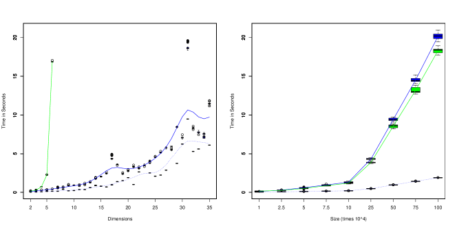
The evolutionary algorithm has many tuning parameters, some of which control its accuracy. As we have seen in Figure 10, the default settings for these tuning parameters are pre-set to deliver fast results. In trade-off for higher computational time, the user can adjust the settings to a more precise algorithm. The key parameters useAllSubsets, nSubsetsUsed, and sigmaLog10Dec. The latter is the main abort criterion of the algorithm. It forces the algorithm to stop if the logarithmized initial variance differs more then the value of sigmaLog10Dec from the actual logarithmized variance. In other words, when the variance of the mutation vector is getting small enough, the algorithm stops.
The settings for useAllSubsets and nSubsetsUsed take control over how many spanned hyperplanes should be taken into account during the calculation of the Oja median. Since the total amount of possible hyperplanes could be huge (it is for observations in the variate case) the flag for useAllSubsets should be used carefully. It is more advisable to control this with the nSubsetsUsed. Raise this value together with sigmaLog10Dec for more precise values, lower them for faster results.
The dynamics of the evolutionary algorithm are controlled via the parameters sigmaInit, sigmaAda and adaFactor. All these take control over the variance adjustments of the mutation vector. The parameter sigmaInit sets the initial variance of the the mutation, the settings for sigmaAda control after how many mutation steps the mutation variance is adjusted and adaFactor defines how the variance is adjusted. In most cases the default settings work nicely.
To conclude this subsection, we would like to mention that there are many R-packages available to compute various medians: The depth package [Genest et al., 2012] contains Tukey’s median, Liu’s median, spatial, marginal, and also the Oja median. The authors use the early Fortran implementation by Niinimaa et al. [1992]. Other packages containing different algorithms to compute the spatial median are, e.g., ICSNP [Nordhausen et al., 2015a], MNM [Nordhausen et al., 2015b, Nordhausen and Oja, 2011] and pcaPP [Filzmoser et al., 2014]. Some of these packages also offer functions for multivariate signs and ranks and methods based upon them.
4.2 Short demonstation of the package’s main function
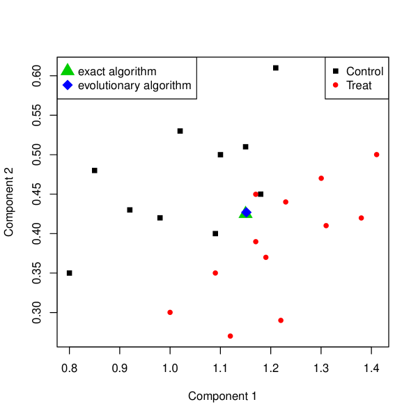
In this section we will demonstrate the main functions of the package using the biochem data set. This data set consists of the amounts of two chemical components in the brain measured at 22 mice. Ten of the mice belong to a control group and twelve received a drug.
This is a very basic example just to demonstrate the basic use of the main functions. For details about the functions see also their corresponding help pages.
We first load the package and the data and create data objects for easier handling as well as fixing the random seed for reproducibility.
> library("OjaNP")> data("biochem")> set.seed(1)> X <- as.matrix(biochem[,1:2])> GROUP <- biochem$group> GRlabel <- as.numeric(GROUP)
Next we compute the bivariate Oja median of the two components using the default evolutionary algorithm.
> OMev <- ojaMedian(X)> OMev
comp.1 comp.2 1.150 0.425
As this toy data set is quite small, it is no problem to compute here also the exact Oja median using either of the algorithms provided.
> OMex <- ojaMedian(X, alg = "exact")> OMex
comp.1 comp.21.1515385 0.4269231
> OMbo <- ojaMedian(X, alg = "bounded_exact")> OMbo
comp.1 comp.21.1515385 0.4269231
As can be seen, the difference between the exact and the approximate estimate is rather small, which is also visualized in Figure 12, produced by the following code:
> plot(X[,1], X[,2], col = GRlabel, pch = GRlabel + 14,+ xlab="Component 1", ylab="Component 2")> points(OMev[1], OMev[2], cex = 2, pch = 17, col = 3)> points(OMex[1], OMex[2], cex = 2, pch = 18, col = 4)> legend("topright", legend = levels(GROUP), col = 1:2, pch = 15:16)> legend("topleft", legend = c("exact algorithm", "evolutionary algorithm"),+ col=3:4, pch = 17:18, pt.cex = 2)
Next we look at the Oja signs of the data.
> head(ojaSign(X))
[,1] [,2] [1,] 0.010681818 0.1150000000 [2,] -0.063181818 0.0295454545 [3,] -0.058409091 -0.0300000000 [4,] -0.058863636 0.0786363636 [5,] -0.063409091 0.0009090909 [6,] -0.015681818 0.1204545455
These signs are computed with respect to the Oja median. But the ojaSign function has several options to compute them also with respect to some other location. For example the vector of marginal medians can be specified as
> head(ojaSign(X, center = "compMedian"))
[,1] [,2] [1,] 0.010681818 0.1145454545 [2,] -0.063409091 0.0195454545 [3,] -0.059772727 -0.0240909091 [4,] -0.058863636 0.0781818182 [5,] -0.063409091 0.0004545455 [6,] -0.015681818 0.1200000000
The Oja signs covariance matrix can be similarly obtained as
> ojaSCM(X)
comp.1 comp.2comp.1 0.0020624226 -0.0004861058comp.2 -0.0004861058 0.0078892444
Next we test whether the Oja median of the control group corresponds to the value c(1,0.5).
> oja1sampleTest(X[1:10, ], mu = c(1,0.5))
OJA 1 SAMPLE SIGN TESTdata: X[1:10, ]Q.S = 3.3745, df = 2, p-value = 0.185alternative hypothesis: true location is not equal to c(1,0.5)
The test decision is here based on the limiting distribution. The sample size is rather small in this example, and one may prefer to use permutation -values. Using the method argument of the function, -values can be computed by permutation.
> oja1sampleTest(X[1:10, ], mu = c(1,0.5), method = "permutation")
OJA 1 SAMPLE SIGN TESTdata: X[1:10, ]Q.S = 3.3745, replications = 1000, p-value = 0.189alternative hypothesis: true location is not equal to c(1,0.5)
To demonstrate the -sample location test, we use the rank test to test whether the two groups differ and want to base the decision on permutation principles.
> ojaCsampleTest(X~GROUP, scores="rank", method = "permutation")
OJA C SAMPLE RANK TESTdata: X by GROUPQ.R = 15.17, permutations = 1000, p-value = 0.001alternative hypothesis: true location difference is not equal to c(0,0)
5 Conclusions
There are many different multivariate medians. In this paper we explained how the different medians extend different properties of the univariate median to the multivariate case. The Oja median has very convincing statistical properties, but is also among the computationally more challenging ones. We described the R-package OjaNP, which provides four different algorithms for its computation. Along with the concept of the Oja median comes the notion of Oja signs and ranks and multivariate scatter estimators based upon them. The package provides also functions for these useful tools, which can then be used for robust multivariate inferential procedures. As examples, we described and implemented the one-sample and the -sample location test based on Oja signs and ranks.
Acknowledgements
The work of Klaus Nordhausen was supported by the Academy of Finland (grant 268703). Oleksii Pokotylo is supported by the Cologne Graduate School of Management, Economics and Social Sciences. The work of Daniel Vogel was supported by the DFG collaborate research grant SFB 823.
References
- Hayford [1902] J. Hayford. What is the center of an area or the center of a population. Journal of the American Statistical Association, 8(58):47–58, 1902.
- Tukey [1975] J. W. Tukey. Mathematics and the picturing of data. In Proceedings of the International Congress of Mathematicians, volume 2, pages 523–531. Vancouver, 1975.
- Weber [1909] Alfred Weber. Über den Standort der Industrien. Mohr, Tübingen, 1909.
- Weber [1929] Alfred Weber. Theory of the Location of Industries. The University of Chicago Press, Chicago, 1929.
- Small [1990] Christopher G. Small. A survey of multidimensional medians. International Statistical Review, 58(3):263–277, 1990.
- Oja [2013] Hannu Oja. Multivariate median. In Claudia Becker, Roland Fried, and Sonja Kuhnt, editors, Robustness and Complex Data Structures. Festschrift in Honour of Ursula Gather, pages 3–16. Springer-Verlag, Berlin, 2013.
- Oja [1983] Hannu Oja. Descriptive statistics for multivariate distributions. Statistics & Probability Letters, 1(6):327–332, 1983. doi: 10.1016/0167-7152(83)90054-8.
- Fischer et al. [2016] Daniel Fischer, Karl Mosler, Jyrki Möttönen, Klaus Nordhausen, Oleksii Pokotylo, and Daniel Vogel. OjaNP: Multivariate Methods Based on the Oja Median and Related Concepts, 2016. URL https://CRAN.R-project.org/package=OjaNP. R package version 0.9-9.
- R Core Team [2016] R Core Team. R: A Language and Environment for Statistical Computing. R Foundation for Statistical Computing, Vienna, Austria, 2016. URL https://www.R-project.org/.
- Hotelling [1929] Harold Hotelling. Stability in competition. The Economic Journal, 39(153):41–57, 1929. doi: 10.2307/2224214.
- Donoho and Gasko [1992] D. Donoho and M. Gasko. Breakdown properties of location estimates based on half-space depth and projected outlyingness. The Annals of Statistics, 20(4):1803–1827, 1992.
- Chen [1995] Zhiqiang Chen. Robustness of the half-space median. Journal of Statistical Planning and Inference, 46(2):175–181, 1995.
- Stein [1966] P. Stein. A note on the volume of a simplex. The American Mathematical Monthly, 73(3):299–301, 1966. doi: 10.2307/2315353.
- Niinimaa [1995] Ahti Niinimaa. Bivariate generalizations of the median. In E.-M. Tiit, T. Kollo, and H. Niemi, editors, Multivariate Statistics and Matrices in Statistics, pages 163–180. VSP BV, Zeist, 1995.
- Oja [1999] Hannu Oja. Affine invariant multivariate sign and rank tests. Scandinavian Journal of Statistics, 26(3):319–343, 1999.
- Oja and Niinimaa [1985] Hannu Oja and Ahti Niinimaa. Asymptotic properties of the generalized median in the case of multivariate normality. Journal of the Royal Statistical Society B, 47(2):372–377, 1985.
- Arcones et al. [1994] Miguel A. Arcones, Zhiqiang Chen, and Evarist Gine. Estimators related to -processes with applications to multivariate medians: Asymptotic normality. The Annals of Statistics, 22(3):1460–1477, 09 1994.
- Shen [2008] Gang Shen. Asymptotics of oja median estimate. Statistics & Probability Letters, 78(14):2137–2141, 2008. doi: 10.1016/j.spl.2008.02.004.
- Niinimaa and Oja [1995] Ahti Niinimaa and Hannu Oja. On the influence functions of certain bivariate medians. Journal of the Royal Statistical Society B, 57(3):565–574, 1995.
- Niinimaa et al. [1990] Ahti Niinimaa, Hannu Oja, and Mara Tableman. The finite-sample breakdown point of the oja bivariate median and of the corresponding half-samples version. Statistics & Probability Letters, 10:325–328, 1990. doi: 10.1016/0167-7152(90)90050-H.
- Babu and Rao [1988] G. Jogesh Babu and C. Radhakrishna Rao. Joint asymptotic distribution of marginal quantiles and quantile functions in samples from a multivariate population. Journal of Multivariate Analysis, 27(1):15–23, 1988. doi: 10.1016/0047-259X(88)90112-1.
- Romanazzi [2001] Mario Romanazzi. Influence function of halfspace depth. Journal of Multivariate Analysis, 77(1):138–161, 2001. doi: 10.1006/jmva.2000.1929.
- Bai and He [1999] Zhi-Dong Bai and Xuming He. Asymptotic distributions of the maximal depth estimators for regression and multivariate location. The Annals of Statistics, 27(5):1616–1637, 1999.
- Möttönen et al. [2010] Jyrki Möttönen, Klaus Nordhausen, and Hannu Oja. Asymptotic theory of the spatial median. In J. Antoch, M. Hŭsková, and P. K. Sen, editors, Nonparametrics and Robustness in Modern Statistical Inference and Time Series Analysis: A Festschrift in Honor of Professor Jana Jurecková, volume 7, pages 182–193, 2010.
- Hettmansperger and McKean [2011] Thomas P. Hettmansperger and Joseph W. McKean. Robust Nonparametric Statistical Methods. CRC Press, Boca Raton, 2nd edition, 2011.
- Puri and Sen [1971] M. L. Puri and P. K. Sen. Nonparametric Methods in Multivariate Analysis. WileyJohn Wiley & Sons, New York, 1971.
- Oja [2010] Hannu Oja. Multivariate Nonparametric Methods with R. An Approach Based on Spatial Signs and Ranks. Springer-Verlag, New York, 2010.
- Visuri et al. [2000] Samuli Visuri, Visa Koivunen, and Hannu Oja. Sign and Rank Covariance Matrices. Journal of Statistical Planning and Inference, 91(2):557–575, 2000.
- Ollila et al. [2003] Esa Ollila, Hannu Oja, and Christophe Croux. The affine equivariant sign covariance matrix: Asymptotic behavior and efficiencies. Journal of Multivariate Analysis, 87(2):328–355, 2003. doi: 10.1016/S0047-259X(03)00045-9.
- Visuri et al. [2003] Samuli Visuri, Esa Ollila, Visa Koivunen, Jyrki Möttönen, and Hannu Oja. Affine Equivariant Multivariate Rank Methods. Journal of Statistical Planning and Inference, 114(1-2):161–185, 2003. doi: 10.1016/S0378-3758(02)00469-X.
- Ollila et al. [2004] Esa Ollila, Christophe Croux, and Hannu Oja. Influence function and asymptotic efficiency of the affine equivariant rank covariance matrix. Statistica Sinica, 14(1):297–316, 2004.
- Vogel et al. [2008] D. Vogel, C. Köllmann, and R. Fried. Partial correlation estimates based on signs. In J. Heikkonen, editor, Proceedings of the 1st Workshop on Information Theoretic Methods in Science and Engineering. TICSP series # 43, 2008.
- Vogel and Fried [2008] D. Vogel and R. Fried. Estimating partial correlations using the oja sign covariance matrix. In P. Brito, editor, Compstat 2008: Proceedings in Computational Statistics. Vol. II, pages 721–729. Heidelberg: Physica-Verlag, 2008.
- Vogel and Fried [2011] D. Vogel and R. Fried. Elliptical Graphical Modelling. Biometrika, 98(4):935–951, 2011.
- Hettmansperger et al. [1994] Thomas P. Hettmansperger, Jukka Nyblom, and Hannu Oja. Affine invariant multivariate one-sample sign tests. Journal of the Royal Statistical Society B, 56(1):221–234, 1994.
- Hettmansperger et al. [1997] Thomas P. Hettmansperger, Jyrki Möttönen, and Hannu Oja. Affine-invariant multivariate one-sample signed-rank tests. Journal of the American Statistical Association, 92(440):1591–1600, 1997.
- Hettmansperger and Oja [1994] Thomas P. Hettmansperger and Hannu Oja. Affine invariant multivariate multisample sign tests. Journal of the Royal Statistical Society B, 56(1):235–249, 1994.
- Hettmansperger et al. [1998] Thomas P. Hettmansperger, Jyrki Möttönnen, and Hannu Oja. Affine invariant multivariate rank tests for several samples. Statistica Sinica, 8:785–800, 1998.
- Ronkainen et al. [2003] Tommi Ronkainen, Hannu Oja, and Pekka Orponen. Computation of the multivariate oja median. In R. Dutter, P. Filzmoser, U. Gather, and P. J. Rousseeuw, editors, Developments in Robust Statistics: Proceedings of the International Conference on Robust Statistics (ICORS’01, Stift Vorau, Austria, July 2001), pages 344–359. Springer-Verlag, Berlin Heidelberg, 2003.
- Mosler and Pokotylo [2015] Karl Mosler and Oleksii Pokotylo. Computation of the Oja Median by Bounded Search. In Klaus Nordhausen and Sara Taskinen, editors, Modern Nonparametric, Robust and Multivariate Methods, pages 185–203. Springer-Verlag, 2015.
- Niinimaa et al. [1992] Ahti Niinimaa, Hannu Oja, and Jukka Nyblom. Algorithm as 277: The oja bivariate median. Applied Statistics, 41(3):611–633, 1992. doi: 10.2307/2348099.
- Hettmansperger et al. [1999] Thomas P. Hettmansperger, J. Möttönen, and H. Oja. The geometry of the affine invariant multivariate sign and rank methods. Nonparametric Statistics, 11(1-3):271–285, 1999. doi: 10.1080/10485259908832784.
- Genest et al. [2012] Maxime Genest, Jean-Claude Masse, and Jean-Francois Plante. depth: Depth Functions Tools for Multivariate Analysis, 2012. URL https://cran.r-project.org/package=depth. R package version 2.0-0.
- Koenker et al. [2016] Roger Koenker, Stephen Portnoy, Pin Tian Ng, Achim Zeileis, Philip Grosjean, and Brian D. Ripley. quantreg: Quantile Regression, 2016. URL https://cran.r-project.org/package=quantreg. R package version 5.21.
- Nordhausen et al. [2008] Klaus Nordhausen, Hannu Oja, and David E. Tyler. Tools for exploring multivariate data: The package ICS. Journal of Statistical Software, 28(6):1–31, 2008. doi: 10.18637/jss.v028.i06. URL http://www.jstatsoft.org/v28/i06/.
- Nordhausen et al. [2015a] Klaus Nordhausen, Seija Sirkiä, Hannu Oja, and David E. Tyler. ICSNP: Tools for Multivariate Nonparametrics, 2015a. URL https://cran.r-project.org/package=ICSNP. R package version 1.1-0.
- Nordhausen et al. [2015b] Klaus Nordhausen, Jyrki Möttönen, and Hannu Oja. MNM: Multivariate Nonparametric Methods. An Approach Based on Spatial Signs and Ranks, 2015b. URL https://cran.r-project.org/package=MNM. R package version 1.0-1.
- Nordhausen and Oja [2011] Klaus Nordhausen and Hannu Oja. Multivariate methods: The package MNM. Journal of Statistical Software, 43(5):1–28, 2011. doi: 10.18637/jss.v043.i05. URL http://www.jstatsoft.org/v43/i05/.
- Filzmoser et al. [2014] Peter Filzmoser, Heinrich Fritz, and Klaudius Kalcher. pcaPP: Robust PCA by Projection Pursuit, 2014. URL https://cran.r-project.org/package=pcaPP. R package version 1.9-60.