Finite-time Partitions for Lagrangian Structure Identification in Gulf Stream Eddy Transport
Abstract
We develop a methodology to identify finite-time Lagrangian structures from data and models using an extension of the Koopman operator-theoretic methods developed for velocity fields with simple (periodic, quasi-periodic) time-dependence. To achieve this, the notion of the Finite Time Ergodic (FiTER) partition is developed and rigorously justified. In combination with a clustering-based approach, the methodology enables identification of the temporal evolution of Lagrangian structures in a classic, benchmark, oceanographic transport problem, namely the cross-stream flux induced by the interaction of a meso-scale Gulf Stream Ring eddy with the main jet. We focus on a single mixing event driven by the interaction between an energetic cold core ring (a cyclone), the strong jet, and a number of smaller scale cyclones and anticyclones. The new methodology enables reconstruction of Lagrangian structures in three dimensions and analysis of their time-evolution.
pacs:
92.10.ak,92.10.Lq,47.10.Fg,47.27.DeI Introduction
Understanding the Lagrangian transport between distinct flow features is particularly important in the geophysical context where rotation and stratification, coupled with the extreme geometric aspect ratio, produce long-lived, coherent vortices in the horizontal velocity field Provenzale99 . The ‘geometric approach’ to quantifying advective exchange by calculation of Lagrangian transport boundaries, first developed to understand the dynamics of classical Hamiltonian systems, has been both widely used and explicitly developed in context of meso-scale oceanographic and atmospheric flows (see, (Wiggins2005, ; Koshel2006, ; Samelson2013, ) for reviews in the oceanographic context). The need for analysis of geometric structures that organize advection is not purely academic. Predicting rates and pathways of material transport by environmental flows has been an essential element in the response to several recent catastrophic events, namely, the volcanic eruption of Eyjafjallajökull (2010), the Deepwater Horizon oil spill (2010), and the nuclear disaster in Fukushima (2011). These events highlight the importance of detecting organizing geometric structures in (near) real time from data, either measured or generated by detailed simulation models; consequently, such problems have become a very active intersection of dynamical systems and fluid dynamics.
Presently, there exists a large and diverse literature of techniques for detecting, quantifying and visualizing the organizing structures controlling Lagrangian mixing and transport in unsteady, aperiodic flows Gildor2014 . Conceptually, a coherent structure in the Lagrangian frame is a set of similar trajectories, ie trajectories that move together in any inertial reference frame for an extended period of time. Methods for unambiguously defining sets of initial conditions satisfying such criteria, either explicity or by defining the set boundaries, are readily available for autonomous or time periodic flows and rely heavily on studying the geometry of invarient manifolds defined by asymptotic time properties. The theory of Lagrangian Coherent Structures Haller2005 (LCS) identifies barriers that organize the transport in flows with complex time-dependence. Initially, LCS were closely associated with computation of Finite-Time Lyapunov Exponent fields Shadden2005 ; more recently, they have been re-formulated using a variational principle Haller2011a ; Haller2012 ; Blazevski2014 , which defines them as certain geodesic lines of the local deformation field induced by the fluid flow. This new definition allows a finer classification of LCS, both in two- and three-dimensions, based on the type of deformation, e.g., hyperbolic, elliptic, corresponding to different behaviors of fluid parcels in the flow. The recent review by Haller Haller2015 gives a detailed coverage of the current state-of-the-art in the LCS theory.
Magnitudes of the local material deformation are typically estimated by processing velocity gradient information and typically difficult to compute precisly in the absence of the detailed data about the velocity field, e.g., when the system is sampled only by sparse trajectories or the underlying velocity field is noisy or underresolved. To avoid this, alternate measures to local deformation gradient information have been proposed as bases for defining coherent stucture boundaries rypinaetal:2011 ; manchoetal:2013 . In sparsely-sampled planar systems, trajectories can be represented by space-time braids — extremely-reduced, symbolic representations of trajectories. The resulting approach, known as braid dynamics Boyland2000 ; Allshouse2012 ; Thiffeault2010 has been successful in providing lower bounds on the amount of deformation present in the flow in limited-data settings. The obtained bounds have been used both in design and analysis of the material advection; unfortunately, there are currently no extensions of braid dynamics to three-dimensional flows.
Instead of looking for barriers to transport (boundaries of coherent sets), as is the case with the LCS theory, the theory of almost-invariant sets attempts to directly identify a collection of sets, fixed in initial condition space, such that the exchange of material between these set is minimized under the action of the flow over a finite time. These sets act as routes for the material transport. The approach is based on the Perron-Frobenius transfer operator, which models how the flow moves distributions of points, instead of individual trajectories. The Perron-Frobenius operator is always infinite-dimensional and linear; the identification of almost-invariant sets is then intimately connected with approximating its eigenfunctions. In practice, the Perron-Frobenius operator is approximated by a finite dimensional transfer operator produced by binning initial conditions. While the Perron-Frobenius operator has been a staple of the ergodic and probability theory since the early 20th century, it was introduced to applied, non-probabilistic context by Dellnitz and collaborators Dellnitz1999 ; Dellnitz2002 as the basis for identification of invariant sets in time-invariant dynamical systems. The theory has since been expanded to include detection of almost-invariant sets of autonomous systems Froyland2003 ; Froyland2009 , and flows with more general time dependencies including applications to geophysical transport Froyland2010 ; Froyland2010a ; froyland2015 .
Spatial invariants of dynamical systems are directly related to infinite-time averages of functions along Lagrangian trajectories via ergodic theory Mezic:1994 . In this context, evidence exists that even finite-time averages of functions can enable detection of geometric structures important for fluid transport Poje1999 . The utility of time-averages has been corroborated on numerical and experimentally-realizable flows with simple time dependenceMezic1999 ; Malhotra1998 ; Mezic2002 . Computations of (approximately) ergodic invariant sets using long-time averages of a large set of averaged function have been investigated Mezic:1994 ; Mezic1999 ; Levnajic2010 ; Budisic2012b and the connection between these approaches and LCS theory has recently been made Farazmand2015a .
Here we concentrate on the approach established in Mezic:1994 ; Mezic1999 ; Levnajic2010 ; Budisic2012b to extend the theory based on finite-time Lagrangian averages of the velocity field. We make an explicit connection with the Koopman operator theory that describes evolution of observables under dynamics of flows MezicandBanaszuk:2004 ; Mezic:2005 ; Mezic:2013 . For observables, we use fixed sets of basis functions combined with machine learning (standard high-dimensional clustering algorithms) in order to determine finite-time structures within which the trajectories themselves possess most similar statistics. The goal is to develop a robust procedure for identifying structures that (1) requires only Lagrangian position data as input (2) is based on global properties of the full set of available trajectories and (3) naturally extends to three dimensional velocity fields.
Specifically, we seek to elucidate the time dependence of interacting coherent mesoscale features (spatial scales 10km) in a highly resolved, highly time dependent, submesoscale-eddy-permitting model of the Gulf Stream. To date, the majority of Lagrangian coherent structure applications in geophysical flows have considered meso-scale dominated velocity fields either produced by relatively coarsely resolved/idealized models Miller:1997 ; Lipp08 ; Bettencourt2012 ; Pratt2014 or derived directly from available remote sensing data using geostrophy Ngan1999 ; Ovidio:2004 ; Beronvera2008 . In contrast to these fields which necessarily impose a rapid fall-off of energy at small spatial scales, current ocean models produce distinct signatures of submesocale turbulence, with broad wavenumber and frequency spectra, as model resolution is increased towards 1km Capet2008a ; Bracco2016 . A primary goal here is to demonstrate the ability of time-averaged, cluster-based partitions to identify dominant three-dimensional mesoscale mixing structures in the presence of significant small scale fluctuations. The specific problem, quantifying eddy-induced mixing between and across the Gulf Stream, was the original motivation for many LCS studies BowRos85 ; Samels91 ; DutPal94 and has received considerable attention SonRos95 ; Rog99 ; Yuan2002 ; Budyansky2009 .
The paper is organized as follows: In section II we discuss the model velocity field and transport geometry. In section III we discuss the Koopman operator approach to visualization of Lagrangian structures and discuss the selection of observables. In section IV we introduce the notion of Finite-Time Ergodic (FiTER) Partition and present results on identification of Lagrangian coherent structures using a clustering algorithm. In section V we discuss how the technique of FiTER partition, together with the clustering algorithm enables reconstruction of three-dimensional Lagrangian structures and analysis of their evolution in time. We conclude in section VI. In the Appendix, we provide the rigorous theory of FiTER partitions and define the associated measure-theoretic notions of almost invariant sets and maximally coherent sets.
II Numerical Model
II.1 HYCOM numerical simulation for the North Atlantic
The Hybrid Coordinate Ocean Model (HYCOM) bleck02 ; halliwell04 ; chassignet06 is used to numerically simulate the Gulf Stream region. The resulting database corresponds to a high-resolution subdomain with a Mercator grid resolution of () spanning W N to W N (see Fig. 1). The vertical spatial discretization consists of 30 hybrid (z-sigma-isopycnal) layers of which the top six are in coordinates while the ocean interior is discretized in potential density coordinates. The high-resolution subdomain is one-way nested within a coarse grid () run covering the Atlantic Ocean and the Mediterranean Sea in the latitudinal range S and N. The fine grid simulation, initialized using the results from a 8 year long coarse grid run, is evolved for a total span of 501 days. After discarding the initial 134 days to minimize the effects of re-gridding, the complete database catalogs flow evolution over one whole year starting on May 15 (day 1 hereafter). The model data is identical to that described in (mensa2013, ) to which the reader is referred for dynamical details. In terms of Gulf-Stream characterization, velocities and eddy kinetic energy, the numerical results are consistent with drifter data analysis (fratantoni01 ; garraffo01 ; lumpkin13 ). Similarly, the sea surface height variability is the Gulf Stream extension is in agreement with altimeter data ducet00 .
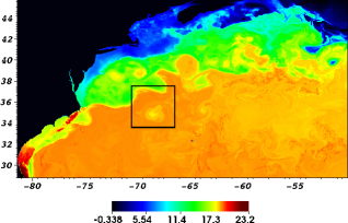
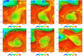
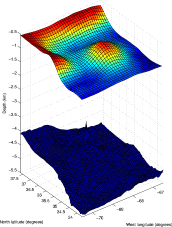
We are interested in elucidating the evolution of coherent structures and their associated transport where the meandering Gulf Stream generates strong mesoscale flow features. Such conditions are found throughout, but we concentrate on a specific event during the summer (day 70 to day 125) in the subregion defined by the corners and shown in Fig. 1 as a black square. The projection of this domain roughtly corresponds to an extent of . Several HYCOM snapshots of instantaneous velocity and salinity for this temporal and spatial domain of interest are shown in Fig. 2. The domain is approximately centered on a strong cyclonic, ‘cold-core’ ring located south of the Gulf Jet Stream characterized by strong eastward currents and low salinity. The cold-core ring persists as a coherent feature over the 25 day time span, interacting with the meandering jet and smaller scale anti-cyclonic structures throughout this time. The lower vertical boundary of the domain of interest is given by the 23rd isopycnal model layer, shown for day 80 in Fig. 3 along with the bathymetry, characterized by the Caryn Seamount rising approximately 2,000 meters above the Sohm abyssal plain.
II.2 Synthetic trajectories
The Lagrangian data is given by trajectories of 90,000 synthetic drifters, initialized at various times on a uniform 300 300 horizontal grid spanning the domain of interest in each of the 23 isopycnal layers considered. The trajectories are computed by integrating for each isopycnal level over the time interval . The integration scheme used is fourth order Runge-Kutta and each particle velocity is obtained via linear temporal interpolation between consecutive 12-hour HYCOM velocity fields and third order spline interpolation in both spatial directions.
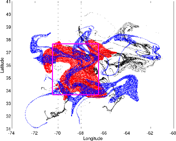
Fig. 4 shows the position of the full set of drifters on the uppermost (black) and lowest (red) isopycnals after 7 days. The magenta lines mark the location of the initial patch. For fixed integration time, particles in the lowest isopycnal travel much less than those in the uppermost level as a result of the large diapycnal (vertical) shear of the along-isopycnal velocities.
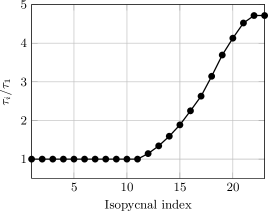
As explained below, the approach used to organize the complexity of the full set of trajectories across isopycnals is based on computing time averages of sets of spatially dependent functions. The disparity in Lagrangian averages on different layers can be accounted for either by explicitly choosing the layer (depth) dependence of such functions a priori, or by considering identical sets of functions at each isopycnal and adjusting averaging times accordingly. For simplicity of presentation, we choose the latter approach and rescale integration times across isopycnals to ensure that the average length of trajectories are equal. The temporal rescaling used throughout is shown in Fig. 5. The effect on the trajectories is illustrated in Fig. 4 where the final positions of the day trajectories in the lowest isopycnal are shown in blue. Under this temporal rescaling, the average length of trajectories in the lowest (blue) and the topmost (black) layers are commensurate.
III Observables: Lagrangian time-averaged basis functions
Approaches based on the Koopman operator have been successfully used to analyze dynamical systems that, because of their high-dimensionality, ill-description and uncertainties, were not well posed for the classical Poincaré approach based on the concept of ‘dynamic of states’ budisic12 . The Koopman approach, based on the ‘dynamics of observables’, has demonstrated to be a well-suited alternative to overcome these difficulties which frequently appear in current engineering and big data applications including fluid dynamics in turbulent flows and Unmanned Aerial Vehicle operations.
In the typical setting, the dynamics on a state space or closed domain is set by an iterated map or flow such that . An observable on this state space consists in a function where is an element of a function space . Conceptually, an observable can be described as a probe under the action of the dynamical system that stores not just the trajectory but the trace . The Koopman operator, , can then be defined as
| (1) |
i.e. the composition of the observable and the iterated map . Typically we only have access to a limited collection of observables, , that can represent some relevant set for the specific problem or a function basis for . As such, if , then the Koopman operator is defined as:
| (2) |
In the case of flows with time-dependence, we define a family of Koopman operators parametrized by the initial time and the final time in the interval . It turns out that time-average of the observables along the trajectories in the finite-time interval can be represented as the average action of this family of operators on the observable
and these are in turn described by Dirac measures on trajectories .This is very similar to the process in which ergodic measures are associated with infinite time averages in steady flows Mezic:1994 (see the Appendix for a more precise description).
The ocean model flow fields considered here present two, inter-connected, challenges to to directly applying Koopman operator based partitions to the synthetic drifter data. First, the domain of initial conditions, , that we wish to consider represents a (small) bounded subset of the full North Atlantic simulation () and is not closed under the flow. For finite time trajectories, we must consider where , i.e. maps trajectories outside the initial domain . This implies some reconsideration of the shape and spatial extent of the functions typically used in the necessarily finite basis set. Secondly, the model velocity field is time-dependent but not periodic and consequently there is no single, well defined, averaging period to separate fields into mean and fluctuating components. Equivalently, the aperiodic flow-field defines an an infinite set of finite-time maps, , parameterized by the finite-time flow interval considered. Since the maps cannot be iterated, both the extent to which trajectories explore the full domain and basis-function averages will depend intimately on the averaging time used.
III.1 Basis functions
For simplicity of interpretation, we consider a finite set of basis functions given by an extension of the Haar wavelet form, :
| (3) |
where the domain of interest has been rescaled such that and
and controls the smoothness of the final form of the 2D Haar functional. The observable is then defined as:
| (4) |
where is the particle position, is the integration time period for isopycnal , is the wavelength and sets, in each direction, the even and odd parity of the function.
To check the sensitivity of the ultimate partition approach to the starting choice of basis set, we will also consider harmonic bases, , where instead of the wavelength set by we use the wavenumber :
| (5) | |||
| (6) |
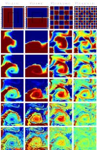
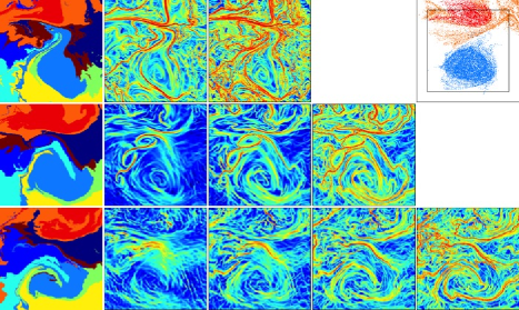
The top row in Figure 6 shows four, Haar-based, functions defined by choosing , , and in Eq. (3). The smoothing parameter has been set to and the rescaled initial domain is indicated as a black square. The choice allows for basis elements with support extending beyond , potentially useful in this open flow situation.
III.2 Dependence on averaging time
The same basis functions, Lagrangian averaged over times and 32 days, are shown in rows 2-6 respectively of Fig. 6. All data corresponds to model layer 12, slightly below the surface layers, but well above the depth of the model Gulf Stream. For the shortest averaging times , and this tendency is more pronounced for functions with larger spatial extent. As the averaging time increases, finer scale features emerge in the observables, with each providing Euelrian frame information about the temporal evolution of Lagrangian trajectories. For days, the large wavelength observables clearly show the existence of a coherent cyclonic eddy core detraining particles to the retrograde motion south of the main jet. Similar time averages of the smaller spatial-scale basis functions, in particular , reveal the existence of anti-cyclonic flow-features on the jet-side of the main cold-core ring.
The evolution of any observable with averaging time provides information about both the time-scales of the Lagrangian motion within individual structures and the non-autonomous time-dependence of the structures themselves. As seen in the bottom row of Fig. 6, long-time averages of smaller spatial scale functions converge to uniform, zero-mean fields while averages of spatially extended modes develop very fine-scale spatial filamentation. In non-autonomous, finite-time flows, the choice of averaging time for the observables is essentially equivalent to the choice of integration time in Finite-Time or Direct Lyapunov Exponent, or Mesohyperbolicity based LCS methods (see, for example, the results shown in Figs. 12 and 13).
The choice of optimal averaging time is subjective and depends on the time dependence of the flow and the ultimate degree of spatial feature resolution sought. In the following we seek to combine information from a fixed set of observables to partition the full 3D+1 flow field. Fixing the smallest spatial scale basis functions to be (nominally probing features with spatial scales 1/4 of the horizontal domain of interest), then the results in Fig. 6 indicate that the choice days is both long enough to allow the emergence of structure information in this observable and short enough to avoid homogenization. This choice of integration time also reduces the degree of filamentation in the larger wavelength observables. The temporal evolution of the eddy shown in Fig. 2 indicates that days is an intermediate time scale for the flow field. Particles sample several rotation periods of the eddy and travel significant distances in the jet during this time period where the structures themselves have evolved more slowly.
III.3 Depth Dependence
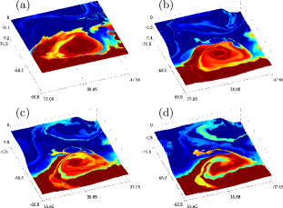
With the temporal rescaling shown in Fig. 5, a single horizontal basis function can be used to explore the evolution of the coherent features throughout the water column. With set to 8 days, the results for the averages of at four different isopycnal layers are shown in Fig. 7. Layer number increases from (a) to (d).
The observable indicates the persistence of the cyclonic feature with increasing depth. While there is a clearly defined core near the surface, this feature is increasingly filamented in the lower layers. The nearly elliptical surface expression evolves into a arrowhead shape at layer 18 indicating entraining lobes of cyclonic trajectories along the southern edge of the ring (red) and detraining trajectories (yellow and green) from the core. As expected, extreme vorticity gradients associated with the Gulf Stream in the upper layers produce a strong transport barrier. With increasing depth, this barrier is weakened as revealed by the presence of cross-jet transport pathways in the time averaged function. These pathways appear to be connected to the appearance, at intermediate layers, of smaller-scale anti-cyclonic features on the jet-side of the cyclone. Overall, the single observable indicates evolution from a relatively isolated cyclonic feature at the surface to a complex multi-pole structure at depth.
IV Partition
As shown above, the Lagrangian statistics of individual basis functions provide detailed information on the location, spatial extent and advective connections between coherent structures in the flow field. The goal here is to combine the complimentary information provided by a collection of functions to partition the initial condition domain into discrete sets within which trajectories possess ‘most similar’ statistics over the set of observables.
The finite-time/open-flow nature of the oceanic transport problem poses questions for application of standard ergodic partition approach. For a dynamical system defined by a (Poincaré) map on a closed domain, ergodic theory allows one to compute the convergence properties of time averages of observable functions (see discussion in levnajic10 ). In the ocean flow, however, there is no well defined, long-time average and, even if there were, one is typically not interested in transport on such long times. In the appendix we develop the mathematical formalism of Finite-Time Ergodic (FiTEr) partitions. A FiTEr partition associated with a finite set of functions is the partition of into joint level sets of . We approximate these joint level sets using clustering algorithms from machine learning.
Using the Haar-like functions, , as basis-set elements and accounting for the lack of orthogonality on when , we will consider sets of functions such as those given in Table 1. This 24 dimensional basis set is obtained by selecting and eliminating the mean mode, and any redundancies produced by symmetry. Such collections are the Haar equivalents of standard discrete Fourier bases and similar sets can be produced by varying the choice of .
| - | 1 | 2 | 3 | 4 | ||
| 5 | 6 | 7 | 8 | 9 | ||
| 10 | 11 | 12 | 13 | 14 | ||
| 15 | 16 | 17 | 18 | 19 | ||
| 20 | 21 | 22 | 23 | 24 | ||
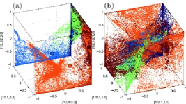
Given a set of functions, each of the 90,000 drifters advected in each of the isopycnals, i.e. trajectories, produces a single point in the space of observables. Using the set of 24 functions given in Tab. 1, samples of the cloud of data points, indicated by small colored points, are shown in Fig.8 in two, 3D projections of . The specific function triplets defining the projections, , , and , , are marked in blue and red in Tab. 1.
The distribution of data in clearly organized and non-uniformly distributed in . Fig. 8a, the projection on quasi-meridional modes (), shows alignment of the data cloud on distinct planes. Values of the odd, , mode concentrate almost entirely on except where the even mode . The projection on observables with smaller spatial scale (Fig. 8b), while more complex, continues to show organization of the data on lower dimensional subspaces of .
IV.1 -means clustering
We seek to define a partition of based on the distribution of the data points in the dimensional space of observables. In other words, we seek to group the points into clusters, such that the statistics defined by the observables in each cluster are closer to each other than to those in other clusters. A standard data-mining cluster algorithm is provided by the -means method. The algorithm aims to partition the data points into clusters so that the within-cluster sum of the squared Euclidean distance between each point and the cluster centroid is minimized. Specifically, we use a standard -means implementation provided by the Statistics and Machine Learning MatLab toolbox. The algorithm is initialized using a subsample of the data, randomly selected according to a previously fixed seed for reproducibility. To ensure that the results are independent of the initialization, the procedure is repeated several times with different initial estimatess for the centroids.
Results of the -means algorithm for clusters are shown in Fig. 8 where the individual data points have been color-coded based on cluster index and the projections of the cluster centroid locations are marked by large, solid spheres. The corresponding partition of in physical space for isopycnal layer 15 is given in Fig. 9a.
IV.2 Convergence properties
The ultimate -means based partition of depends on the number of clusters sought, , and both the dimensionality, , and the specific spatial form of the input basis set of observables.
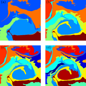
Fig. 9 shows the dependence, for fixed isopycnal layer 15, of the partition on the number of clusters used. Each frame corresponds to partitions of the Haar basis set with . The main cyclonic eddy, previously identified in individual observables, is clearly delineated in each partition. Each partition also clearly identifies coherent anti-cyclonic sets on the jet side of the cyclone. Increasing the number of clusters simply refines the partition by dividing existing features into distinct subsets. For , the main cyclonic eddy (light blue) has both a thin entraining lobe surrounding the anti-cyclone and a larger detraining region to the southwest. For clusters, the detraining region forms a new (yellow) cluster and the definition of the cold-core ’eddy’ is refined. Similar refinement of the detrainment region and the eddy core takes place when increases from 9 to 13. In this sense, for fixed , the resulting partition is stable with respect to the number of clusters; effectively sets the spatial scale of the resulting coherent sets. Again, for simplicity of interpretation of the time dependent, three-dimensional (3D+1) results, we take in what follows.
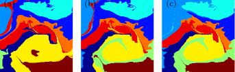
The function set presented in Tab. 1 can be modified by altering the choice of used to define the basis. Fig. 10 shows a comparison at isopycnal of the partition for 8, 24 and 48 dimensional function sets generated by choosing and . As such the 8 dimensional set is a proper subset of the 24 dimensional set which in turn is a proper subset of the 48 dimensional set. Convergence of the large scale structures with the number of Haar basis elements is apparent. The results shown in Fig. 6 indicate that even moderate spatial scale observables are homogenized by representative temporal averages. As such, including smaller scale features in the functional basis has a nominal effect on the main coherent features identified by the global -means partition.
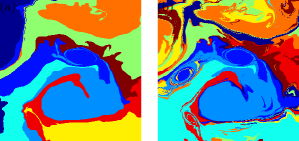
As a further test of the sensitivity of the overall partition to the details of the space of observables, we also consider a standard, harmonic plane wave basis (see Eq. 6). A comparison of the -means partition for 24 dimensional Haar and 16 dimensional harmonic set is shown in Fig. 11. The harmonic set corresponds to where the has been discarded. Note that each pair of wavenumber values () has associated two solutions for the real and imaginary parts of the harmonic function.
Again, the overall partition, especially the shape and location of the coherent cold-core eddy, is remarkably insensitive to the functional form of the basis. The major difference between the harmonic functions and the Haar functions is the density distribution of the range of the functions. By construction, the range of the Haar functions is concentrated at . As seen in the figure, the broader distribution of the range of the harmonic functions produces, for fixed averaging time, a more detailed, finer spatial scale, picture of the flow field.
IV.3 Depth dependence: Comparison to LCS metrics
For a given initialization time, the partitions result from -means clustering of the full Lagrangian data set across all 23 isopycnal levels. The depth dependence of the coherent sets produced by the , partition is shown at three representative isopycnal levels in the first columns of Figs. 12 and 13. Here the model trajectories were launched on day 74.
The -means partition provides considerable refinement of the depth dependence of the main cyclonic structure shown previously, for a single observable initialized on day 80, in Fig. 7. In the near-surface, the cold-core ring at day 74 (light blue) is entraining fluid along a thin filament on the southern side of the jet and the transport geometry is similar to that of ’eddy pinch-off’ processes previously observed in simplified, analytic and low-resolution models DutPal94 ; poje99 of eddy-jet interactions. At mid-depth, the entrainment from the jet is impeded by the appearance of a binary pair of smaller scale, anti-cylonic eddies (medium blue) in the region between the jet and the cyclone. The main cyclonic feature is now filamented by detraining lobes of fluid (light blue, yellow). At depth, the main core continues to shrink in size, developing into a arrowhead or mushroom shape usually associated with vortex dipole configurations.
Also shown in Figs. 12 and 13 are direct comparisons between the partitions derived from -means clustering of Lagrangian averaged observables and more traditional Lagrangian Coherent Structure identification metrics, namely the forward time Mesohyperbolicity field Mezic2010 and the field of forward-time Direct Lyapunov Exponents Haller2002 . Both metrics have been widely used to analyze Lagrangian oceanographic transport Waugh2008 ; Beron2008 ; Mezic2010 .
Following Haller2002 , the maximal finite-time Direct Lyapunov Exponent is given by
| (7) |
where is the maximal eigenvalue of the Cauchy-Green strain tensor, , the symmetrized gradient of the flow with respect to initial conditions.
Alternatively, LCS features can be extracted by constructing the mesohyperbolicity field, , over initial conditions defined by
| (8) |
where is the average Lagrangian velocity on starting from . Note that, when , the mesohyperbolicity reduces to the well-known, Eulerian Okubo-Weiss criterion.
Like the Lagrangian averaged observables, both the DLE and mesohyperbolicity metrics depend explicitly on trajectory integration time. This dependence is shown across columns for the 3 ispocynal layers in Figs. 12 and 13.
The distinct differences between the cluster-based partition, arrived at by globally searching for coherent sets across all trajectories, and the LCS approaches based entirely on local trajectory information are apparent in the comparisons. The highly time-dependent velocity fields, generated by a model resolving the largest submesoscale flow dynamics, produces complex spatial and fields for any reasonable integration period. While the main coherent structures, such as the cold-core eddy and associated smaller-scale anti-cyclones are revealed by the maps of both and , the boundaries of these structures and the advective pathways connecting them are obscured by the rich complexity and filamentation of the LCS fields. With a broad range of energetic spatial scales, advective transport both within and between the time-dependent mesoscale structures is modulated by the presence of smaller features with shorter lifetimes resulting in extreme tangling of the finite-time hyperbolic sets organizing the advection.
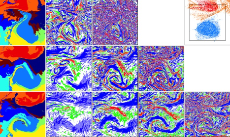
To illustrate the connection between the finite-time partition at the surface and particle behavior, trajectories associated with 3 clusters are shown in the far right top panel in Fig. 12 and 13. The clusters chosen correspond to the main cyclone (light blue partition) and two groups of initial positions in the jet (red and orange). Particles were released on day 74 and advected over the averaging period (7 days). The results clearly show that all initial conditions associated with the light-blue cluster, even those in the entraining lobe, exhibit strong cyclonic circulation during the averaging period. In the jet region, the clustering algorithm distinguishes initial conditions with strongly anti-cyclonic swirl (red) from those that advect with the jet without being entrained into an eddy (orange).
V 3D+1 reconstruction: Temporal evolution of partition
As seen above, even when working in an isopycnal setting, piecing together the depth dependence of coherent features from discrete vertical sets of or fields is difficult. In contrast, the -means partitions, as defined here, directly incorporate information from all layers and produce fully three-dimensional partitions at any initialization time. To investigate the temporal evolution of the features, one need only to reproduce the analysis for a series of launch dates.
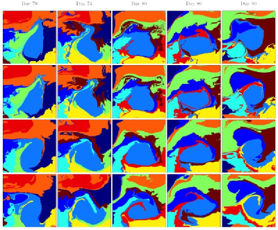
Fig. 15 shows the time and depth dependence of the and partition at four different isopycnal layers (rows) for five different initialization times (columns).
The cyclonic eddy (light blue) partition deforms and rotates under the action of the jet (red/orange for days and orange/green for ). The results for the top isopycnal reveal that for days the upper lobe of the cold core weakens indicating a suppression of the entrainment that is complete at day 86. This event is accompanied by the emergence of anticyclonic structures (dark blue and cyan partitions) in the upper and lower sides of the cyclonic eddy that exhibit respective entraining lobes as observed at day 90. While the spatial extension of the anticyclonic eddy in the north side grows moderately in the vertical at days 70-80, later launch times partitions reveal much stronger reinforcements. For instance, at day 86 the entraining lobe of the dark blue partition strengthens as depth increases and at day 90 the structure resembles that of a dipole with comparable sizes of the partitions for the cyclone and the anticyclone. On the other hand, the second anticyclone structure (cyan) clearly observed at the surface on day 90 vanishes rapidly in the vertical.
In general, the results for the vertical evolution the cyclone indicates a reduction in its size in the vertical. On days 70-80 and at the deepest isopycnal level, the partion of the cold-core eddy exhibits a characteristic arrowhead shape generated by the relatively small anticyclonic features. The results suggest that later on these anticyclonic structures grow bottom-up and eventually become large enough to generate a dipole structure clearly observed at day 90.
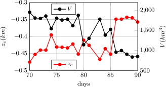
The cold-core ring that spanned across the whole water column for 10 days, decays thereafter indicating the cyclone vertical shrinking. This process is quantified by estimating this structure volume and the vertical location of its centroid as shown in Fig. 14. The results show that as time evolves the cold cyclone size decreases by 50% going from 2,000 to 1,000 cubic kilometers over the span of 20 days. As expected, this volume reduction is accompanied by a reduction in the vertical centroid location.
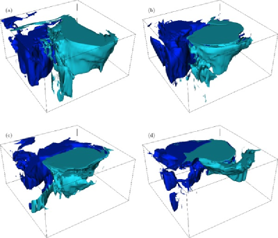
A full picture of the 3D+1 flow evolution in shown in Fig. 16 that contains three-dimensional snapshots of two selected structures at days 73, 78, 84 and 90. Both the vertical shrinking of the cyclonic structure (light blue) and the bottom-up surface emergence of the anticyclone (dark blue) are clearly depicted. These images reveal the extent of both structures and the interaction between them as time evolves. Specifically, it is possible to observe in detail how the anticyclonic core, initially at the deep northwest side of the cold ring, travels in the clockwise direction while resurfaces and impedes the entrainment into the cyclone which then vertically shrinks as shape changes under the action of the jet stream.
VI Conclusions
Transport processes between cold-core eddies and the Gulf Stream has been studied using a novel approach inspired on the Koopman observables. The flow field consists in a HYCOM database of the North Atlantic in which we advect particles at different isopycnal levels. Given a basis set of functions, these observables are obtained by taking time-averages of such functions along particle trajectories advected by the flow field. As in other classical Lagrangian Coherent Structure (LCS) methods, the spatial scale of the flow can be modulated via appropriate integration time.
Once the Lagrangian statistics for the selected integration time span are obtained, the resulting combined high-dimensional space of observables are partitioned using -means. The robustness of such partition was assessed by comparing the results for different number of clusters and basis set definition and dimension. Unlike classic LCS approaches based on local trajectory information on each isopycnal level, the current analysis provides a natural representation of the three-dimensional flow features that can be readily extended to account for temporal dependence by repeating the analysis for different initial ‘particle launch’ dates.
For the specific database used here, the results show that the characteristic lobes of detraining flow on the southern side of the jet eventually are stopped when the mid-depth anticyclonic features growing in the bottom-up direction pinch-off this transport route. At the same time and as the old-core eddy shape changes under the action of the Gulf Stream, its vertical extent shrinks leading to volume reductions of 50% by the end of the 20-day period. At deeper levels, the cold-core topology is observed to evolve from a arrowhead shape to a dipole as the anticyclonic feature grows.
Acknowledgements
This work was partially supported by ONR Grants N00014-11-1-0087 and N00014-14-10633.
VII Appendix: Finite Time Ergodic (FiTEr) partition
In this appendix we define the notion of Finite-Time Ergodic Partition (FiTEr partition) and discuss some of its properties.
We start with a point in a compact domain of the flow, and a sequence of continuous functions . Let
| (9) |
be a vector field on , and its flow where is not necessarily equal to (i.e. trajectories can enter and exit during the time interval of observation). To each point we associate a sequence of numbers defined by
| (10) |
where is the finite-time Koopman operator associated with (9). For fixed and replacing with an arbitrary function , Eq.(10) is a linear functional on the vector space of continuous functions on that, equipped with the Borel -algebra, has a representation as a measure:
| (11) |
In Eq.(11) is the measure that can be thought as a Dirac delta measure on concentrated on the finite time part of the trajectory passing through at and ending at time . The family of measures characterizes the average action in the time interval of the Koopman operator on observables,
Note the similitudes with the ergodic measures (that are eigenfunctions of the Koopman operator adjoint, the Perron-Frobenius operator) for vector fields in Eq.(9) that are independent of Mezic:1994 .
To get an understanding of the measure , we would need to evaluate it on all the continuous functions on , which is unfeasible. Instead, we prove that taking a set of functions whose linear combinations are dense in and evaluating the finite-time averages as defined in (10) leads to a unique determination of the measure :
Theorem 1
Proof Assume not. Then there is a measure s.t. . Consider an arbitrary function . Then there is a sequence of that are linear combinations of such that . Now, each is continuous, and convergence of to the continuous function on compact implies that they are bounded above by some continuous function. By Lebesgue’s Dominated Convergence, then, . But the sequence converges to and thus we get a contradiction.
The result above also has the following simple but important corollary:
Corollary 2
The family of measures does not depend on the chosen set of functions .
Note that, physically, the measure is just the “sojourn measure” that assigns to any open set in the amount of time that the trajectory starting at at time spends in in the period . This leads us to call the family of sojourn measures. In the limit , for steady, periodic or quasiperiodic velocity fields, sojourn measures converge to ergodic measures (see Mezic:1994 for the proof of the ergodic partition theorem that uses the same ideas as above, in the infinite-time limit, and additionally proves ergodic properties of the family of measures thus obtained).
Definition 3
A FiTEr (Finite-Time-Ergodic) partition associated with a finite set of functions is the partition of into joint level sets of .
We remark on two consequences of the above result: 1. the approaches based on integrals of positive functions manchoetal:2013 along a trajectory can fail to uniquely identify underlying objects. Specifically, the notion of Lagrangian descriptors was based on this, but the notion is neither new - as it was proposed much earlier, in Mezic:1994 ; Poje1999 - nor complete, because it does not have the uniqueness property due to choice of only positive functions and 2. attempts to identify invariant structures using averages such as pair dispersion Haller:2015 also suffer from the same non-uniqueness problem.
Farazmand results in farazmand:2015 clarify the relationship between averaging of scalars over Lagrangian trajectories and some of the geometrical approaches. The above measure-theoretic approach shows that single scalar averages are not enough and gives a comprehensive theory, as opposed to geometric approaches. In some cases, even over finite time, sets of points are identified - e.g. for specific times, corresponding to the period, invariant closed curves have the same finite-time averages for all their points. But, in general, it is fruitful to embed the averages into an dimensional space and cluster them, as done in this paper to identify zones with similar trajectory behavior.
Another connection of the this formalism with existing methods can be done as follows: the notion of almost invariant sets has been advanced as a concept that captures fluid parcels traveling together, initially Dellnitz Dellnitz1999 ; Dellnitz2002 . The most recent application of the notion is that of finite-time coherent sets froyland2015 . A metrically invariant set can be defined as a set that satisfies
The above statement just means that the time average on interval of the indicator function of is 1 on almost every trajectory starting in at time zero is 1. Thus, maximally metrically invariant sets are those that satisfy
| (12) |
the exists, where is the Borel -algebra on . Of course, we could ask for the lower bound of the expression and find almost maximally invariant sets, parametrized by the value of . The approach we advanced here can also be used to define finite-time maximally coherent sets via an extremum principle. We say that a set is maximally coherent provided it satisfies
| (13) |
where is some chosen distance on the space of measures (for example the Wasserstein metric), and the factor of in the denominator is due to the fact that . Once again, if does not exist, we could ask for lower bounds, as done above for almost invariant sets. This definition makes sense for a deterministic dynamical system, without any artificial addition of stochastic dynamics as in froyland2015 . It makes intuitive sense, since the idea is that trajectories at and are compared based on their statistical properties - in particular, their finite-time statistics. If those properties are close for a whole set of trajectories starting in then we proclaim that set coherent.
One can develop a multi-scale approach this way, both in space and time, by defining scales in time and in space, using a set of functions of time and space , where is the counter of functions at scale in time, is the counter of functions at scale in space, are centerpoints of functions in the interval of observation and are centerpoints of functions defined on the domain . We form convolution integrals
| (14) |
if there is a countable set of scales in time and space, i.e. a countable set of quantities out of which we can define a trajectory measure at as above. In this paper, we chose to be functions that are constant on subintervals of and as wavelet functions or harmonic functions in space.
References
- (1) A. Provenzale. Transport by coherent barotropic vortices. Annual Rev. Fluid Mech., 31:55–93, 1999.
- (2) S. Wiggins. The dynamical systems approach to Lagrangian transport in oceanic flows. Annual Review of Fluid Mechanics, 37:295–328, 2005.
- (3) K. V. Koshel and S. V. Prants. Chaotic advection in the ocean. Physics-Uspenkhi, 49(11):1151–1178, 2006.
- (4) R. M. Samelson. Lagrangian Motion, Coherent Structures, and Lines of Persistent Material Strain. In Carlson, CA and Giovannoni, SJ, editor, Annual Review of Marine Science, volume 5 of Annual Review of Marine Science, pages 137–163. 2013.
- (5) R. Mundel, E. Fredj, H. Gildor, and V. Rom-Kedar. New Lagrangian diagnostics for characterizing fluid flow mixing. Physics of Fluids, 26(12), 2014.
- (6) G. Haller. An objective definition of a vortex. Journal of Fluid Mechanics, 525:1–26, 2005.
- (7) S. C. Shadden, F. Lekien, and J. E. Marsden. Definition and properties of Lagrangian coherent structures from finite-time Lyapunov exponents in two-dimensional aperiodic flows. Physica D. Nonlinear Phenomena, 212(3-4):271–304, 2005.
- (8) G. Haller. A variational theory of hyperbolic Lagrangian Coherent Structures. Physica D. Nonlinear Phenomena, 240(7):574–598, January 2011.
- (9) G. Haller and F. J. Beron-Vera. Geodesic theory of transport barriers in two-dimensional flows. Physica D: Nonlinear Phenomena, 241(20):1680–1702, October 2012.
- (10) Daniel Blazevski and George Haller. Hyperbolic and elliptic transport barriers in three-dimensional unsteady flows. Phys. D, 273:46–62, 2014.
- (11) G. Haller. Lagrangian coherent structures. Annual Rev. Fluid Mech., 47:137–162, 2015.
- (12) I. I. Rypina, S. E. Scott, L. J. Pratt, and M. G. Brown. Investigating the connection between complexity of isolated trajectories and lagrangian coherent structures. Non-lin. Processes Geophys., 18:977–987, 2011.
- (13) A. M. Mancho, S. Wiggins, J. Curbelo, and C. Mendoza. Lagrangian descriptors: A method for revealing phase space structures of general time dependent dynamical systems. Communications in Nonlinear Science and Numerical Simulation, 18(12):3530–3557, 2013.
- (14) P. L. Boyland, H. Aref, and M. A. Stremler. Topological fluid mechanics of stirring. Journal of Fluid Mechanics, 403:277–304, 2000.
- (15) M. Allshouse and J-L. Thiffeault. Detecting coherent structures using braids. Physica D. Nonlinear Phenomena, pages 95–105, 2012.
- (16) J-L. Thiffeault. Braids of entangled particle trajectories. Chaos: An Interdisciplinary Journal of Nonlinear Science, 20(1):017516–017514, 2010.
- (17) M. Dellnitz and O. Junge. On the approximation of complicated dynamical behavior. SIAM Journal on Numerical Analysis, 36(2):491–515, 1999.
- (18) M. Dellnitz and O. Junge. Set oriented numerical methods for dynamical systems. In Handbook of dynamical systems, Vol. 2, pages 221–264. North-Holland, Amsterdam, 2002.
- (19) G. Froyland and M. Dellnitz. Detecting and locating near-optimal almost-invariant sets and cycles. SIAM Journal on Scientific Computing, 24(6):1839–1863 (electronic), 2003.
- (20) G. Froyland and K. Padberg. Almost-invariant sets and invariant manifolds—connecting probabilistic and geometric descriptions of coherent structures in flows. Physica D. Nonlinear Phenomena, 238(16):1507–1523, 2009.
- (21) G. Froyland, N. Santitissadeekorn, and A. Monahan. Transport in time-dependent dynamical systems: Finite-time coherent sets. Chaos: An Interdisciplinary Journal of Nonlinear Science, 20(4):043116, January 2010.
- (22) G. Froyland, S. Lloyd, and N. Santitissadeekorn. Coherent sets for nonautonomous dynamical systems. Physica D: Nonlinear Phenomena, 239(16):1527–1541, August 2010.
- (23) G. Froyland, C. Horenkamp, V. Rossi, and E. van Sebille. Studying an agulhas ring’s long-term pathway and decay with finite-time coherent sets. Chaos: An Interdisciplinary Journal of Nonlinear Science, 25(8):083119, 2015.
- (24) I. Mezić. On geometrical and statistical properties of dynamical systems: theory and applications. PhD thesis, California Institute of Technology, 1994.
- (25) A.C. Poje, G. Haller, and I. Mezić. The geometry and statistics of mixing in aperiodic flows. Physics of Fluids, 11(10):2963–2968, 1999.
- (26) I. Mezić and S. Wiggins. A method for visualization of invariant sets of dynamical systems based on the ergodic partition. Chaos: An Interdisciplinary Journal of Nonlinear Science, 9(1):213–218, January 1999.
- (27) N. Malhotra, I. Mezić, and S. Wiggins. Patchiness: A New Diagnostic for Lagrangian Trajectory Analysis in Time-Dependent Fluid Flows. International Journal of Bifurcation and Chaos, 08(06):1053–1093, June 1998.
- (28) I. Mezić and F. Sotiropoulos. Ergodic theory and experimental visualization of invariant sets in chaotically advected flows. Physics of Fluids, 14:2235, 2002.
- (29) Z. Levnajić and I. Mezić. Ergodic theory and visualization. I. Mesochronic plots for visualization of ergodic partition and invariant sets. Chaos: An Interdisciplinary Journal of Nonlinear Science, 20(3):–, 2010.
- (30) M. Budišić and I. Mezić. Geometry of the ergodic quotient reveals coherent structures in flows. Physica D. Nonlinear Phenomena, 241(15):1255–1269, August 2012.
- (31) M. Farazmand. Hyperbolic Lagrangian coherent structures align with contours of path-averaged scalars. arXiv:1501.05036 [nlin, physics:physics], January 2015.
- (32) I. Mezić and A. Banaszuk. Comparison of systems with complex behavior. Physica D: Nonlinear Phenomena, 197(1-2):101–133, 2004.
- (33) Igor Mezić. Spectral properties of dynamical systems, model reduction and decompositions. Nonlinear Dynamics, 41(1-3):309–325, 2005.
- (34) Igor Mezic. Analysis of fluid flows via spectral properties of the koopman operator. Annual Review of Fluid Mechanics, 45:357–378, 2013.
- (35) P.D. Miller, C.K.R.T. Jones, A.M. Rogerson, and L.J. Pratt. Quantifying transport in numerically generated velocity fields. Physica D, 110:105–122, 1997.
- (36) B. L. Lipphardt, Jr., A. C. Poje, A. D. Kirwan, Jr., L. Kantha, and M. Zweng. Death of three Loop Current rings. J. Marine Res., 66(1):25–60, 2008.
- (37) J. H. Bettencourt, C. Lopez, and E. Hernandez-Garcia. Oceanic three-dimensional Lagrangian coherent structures: A study of a mesoscale eddy in the Benguela upwelling region. Ocean Modelling, 51:73–83, 2012.
- (38) L. J. Pratt, I. I. Rypina, T. M. Oezgoekmen, P. Wang, H. Childs, and Y. Bebieva. Chaotic advection in a steady, three-dimensional, Ekman-driven eddy. J. Fluid Mech., 738:143–183, 2014.
- (39) K Ngan and TG Shepherd. A closer look at chaotic advection in the stratosphere. Part 1: Geometric structure. J. Atmos Sci., 56(24):4134–4152, 1999.
- (40) F. d’Ovidio, V. Fernandez, E. Hernandez-Garcia, and C. Lopez. Mixing structures in the Mediterranean Sea from finite-size Lyapunov exponents. Geophys. Res. Lett., 31, 2004.
- (41) F. J. Beron-Vera, M. J. Olascoaga, and G. J. Goni. Oceanic mesoscale eddies as revealed by Lagrangian coherent structures. Geophys. Res. Lett., 35(12), 2008.
- (42) X. Capet, J. C. Mcwilliams, M. J. Mokemaker, and A. F. Shchepetkin. Mesoscale to submesoscale transition in the california current system. part i: Flow structure, eddy flux, and observational tests. J. Phys. Oceanogr., 38(1):29–43, 2008.
- (43) Hao Luo, Annalisa Bracco, Yuley Cardona, and James C. McWilliams. Submesoscale circulation in the northern Gulf of Mexico: Surface processes and the impact of the freshwater river input. Ocean Mod., 101:68–82, 2016.
- (44) A. Bower, H. T. Rossby, and J. L. Lillibridge. The Gulf-Stream - Barrier or Blender. Journal of Physical Oceanography, 15(1):24–32, 1985.
- (45) R. M. Samelson. Fluid exchange across a meandering jet. J. Phys. Oceanogr., 21:431–440, 1991.
- (46) S. Dutkiewicz and N. Paldor. On the mixing enhancement in a meandering jet due to the interaction with an eddy. J. Phys. Oceanogr., 24:2418–2423, 1994.
- (47) T. Song, H. T. Rossby, and E. Carter. Lagrangian studies of fluid exchange between the Gulf Stream and surrrounding waters. J. Phys. Oceanogr., 25:46–63, 1995.
- (48) A.M. Rogerson, P.D. Miller, L.J. Pratt, and C.K.R.T. Jones. Lagrangian motion and fluid exchange in a barotropic meandering jet. J. Phys. Oceanogr., 29:2635–2655, 1999.
- (49) G.-C. Yuan, Pratt L. J., and C. K. R. T. Jones. Barrier destruction and lagrangian predictability at depth in a meandering jet. Dynamics of Atmospheres and Oceans, 35(1):41 – 61, 2002.
- (50) M. V. Budyansky, M. Yu. Uleysky, and S. V. Prants. Detection of barriers to cross-jet Lagrangian transport and its destruction in a meandering flow. Physical Review E, 79(5), 2009.
- (51) R. Bleck. An oceanic general circulation model framed in hybrid isopycnic cartesian coordinates. Ocean Modelling, 4:55–88, 2002.
- (52) G. R. Halliwell. Evaluation of vertical coordinate and vertical mixing algorithms in the hybrid coordinate ocean model (hycom). Ocean Modelling, 7:285–322, 2004.
- (53) E. P. Chassignet, H. E. Hurlburt, O. M. Smedstad, G. R. Halliwell, A. J. Wallcraft, E. J. Metzger, B. O. Blanton, C. Lozano, D. B. Rao, P. J. Hogan, and A. Srinivasan. Generalized vertical coordinates for eddy–resolving global and coastal ocean forecasts. Oceanography, 19:20–31, 2006.
- (54) J. A. Mensa, Z. Garraffo, A. Griffa, T. M. Özgökmen, A.C. Haza, and M. Veneziani. Seasonality of the submesoscale dynamics in the Gulf Stream region. Ocean Dynamics, 63(8):923–941, 2013.
- (55) D. M. Fratantoni. North atlantic surface circulation during the 1990’s observed with satellite-tracked drifters. Journal of Geophysical Research: Oceans, 106(C10):22067–22093, 2001.
- (56) Z. Garraffo, A. Mariano, A. Griffa, C. Veneziani, and E. P. Chassignet. Lagrangian data in a high-resolution numerical simulation of the north atlantic: I. comparison with in situ drifter data. J. Mar. Syst., 29:157–176, 2001.
- (57) R. Lumpkin and G. C. Johnson. Global ocean surface velocities from drifters: Mean, variance, el niño–southern oscillation response, and seasonal cycle. Journal of Geophysical Research: Oceans, 118(6):2992–3006, 2013.
- (58) N. Ducet, P. Y. Le Traon, and G. Reverdin. Global high-resolution mapping of ocean circulation from the combination of T/P and ERS-1/2. J. Geophys. Res., 105:477–498, 2000.
- (59) M. Budišić, R. Mohr, and I. Mezić. Applied Koopmanism. Chaos, 22(4), 2012.
- (60) Z. Levnajić and I. Mezić. Ergodic theory and visualization. i. mesochronic plots for visualization of ergodic partition and invariant sets. Chaos, 20:033114, 2010.
- (61) A.C. Poje and G. Haller. Geometry of cross-stream mixing in a double-gyre ocean model. J. Phys. Oceanogr., 29:1649–1665, 1999.
- (62) I. Mezić, S. Loire, V. A. Fonoberov, and P. J. Hogan. A New Mixing Diagnostic and Gulf Oil Spill Movement. Science Magazine, 330(6003):486–489, 2010.
- (63) G. Haller. Lagrangian coherent structures from approximate velocity data. Phys. Fluids, 14:1851–1861, 2002.
- (64) D. W. Waugh and E. R. Abraham. Stirring in the global surface ocean. Geophysical Res. Let., 35(20), 2008.
- (65) F. J. Beron-Vera, M. J. Olascoaga, and G. J. Goni. Oceanic mesoscale eddies as revealed by Lagrangian coherent structures. Geophysical Res. Let., 35(12), 2008.
- (66) A. Hadjighasem, D. Karrasch, H. Teramoto, and G. Haller. A spectral clustering approach to lagrangian vortex detection. arXiv preprint arXiv:1506.02258, 2015.
- (67) M. Farazmand. Hyperbolic lagrangian coherent structures align with contours of path-averaged scalars. arXiv preprint arXiv:1501.05036, 2015.